Analytical Assessment of the Structural Behavior of a Specific Composite Floor System at Elevated Temperatures Using a Newly Developed Hybrid Intelligence Method

Abstract

The aim of this paper is to study the performance of a composite floor system at different heat stages using artificial intelligence to derive a sustainable design and to select the most critical factors for a sustainable floor system at elevated temperatures. In a composite floor system, load bearing is due to composite action between steel and concrete materials which is achieved by using shear connectors. Although shear connectors play an important role in the performance of a composite floor system by transferring shear force from the concrete to the steel profile, if the composite floor system is exposed to high temperature conditions excessive deformations may reduce the shear-bearing capacity of the composite floor system. Therefore, in this paper, the slip response of angle shear connectors is evaluated by using artificial intelligence techniques to determine the performance of a composite floor system during high temperatures. Accordingly, authenticated experimental data on monotonic loading of a composite steel-concrete floor system in different heat stages were employed for analytical assessment. Moreover, an artificial neural network was developed with a fuzzy system (ANFIS) optimized by using a genetic algorithm (GA) and particle swarm optimization (PSO), namely the ANFIS-PSO-GA (ANPG) method. In addition, the results of the ANPG method were compared with those of an extreme learning machine (ELM) method and a radial basis function network (RBFN) method. The mechanical and geometrical properties of the shear connectors and the temperatures were included in the dataset. Based on the results, although the behavior of the composite floor system was accurately predicted by the three methods, the RBFN and ANPG methods represented the most accurate values for split-tensile load and slip prediction, respectively. Based on the numerical results, since the slip response had a rational relationship with the load and geometrical parameters, it was dramatically predictable. In addition, slip response and temperature were determined as the most critical factors affecting the shear-bearing capacity of the composite floor system at elevated temperatures.

1. Introduction

Fire safety is a major concern that has not been well developed in recent years. Many studies have been conducted on a range of approaches to mitigate fire-induced damage to steel and concrete members [1,2,3]. Some research studies have also focused on improving the safety of occupants during and after fire occurrences and on reducing the refurbishment and retrofitting costs.

Composite beams have been widely used in a variety of structures and buildings due to a number of positive features such as lower thickness, considerable span length and high stiffness [4,5]. The development of different composite beams is highly valued to mitigate some shortcomings of specific composite structures [6,7,8]. Steel-concrete composite beams are one of the critical components of high rise and multi-story structures, and different studies have been conducted to improve their performance [9,10]. Moreover, shear connectors (SCs) are one of the most practical elements that are extensively utilized in steel-concrete composite beams to increase shear strength and the integrated behavior of concrete and steel. There are different types of SCs such as channel, angle, stud and perfobond sections. Concrete is cast in different shapes and types such as self-consolidating [11], porous [12], high strength, lightweight and green concrete [13]. Concrete characteristics are divided into two major categories namely fresh and hardened properties. Fresh properties include the most primitive properties of concrete such as slump and workability. On the contrary, hardened properties refer to a range of critical features such as compressive strength, flexural strength, shear strength and corrosion resistance, where many attempts have been made to enhance these properties by surface protection [14,15], the inclusion of fibers and cementitious replacement powders [16].

A few studies have considered push-out tests with various loading patterns to evaluate slip and failure load in channel SCs [17]. Channel SCs have been shown to exhibit ductile performance when exposed to a series of load patterns while equipped with c-shaped connectors; however, this behavior was amplified in more extended channel SCs [18]. In another study, composite beams showed brittle behavior when channel SCs were embedded in plain concrete with no confinement [19]. In contrast, when the channel SCs were embedded in high-strength concrete, the behavior of the composite beam was ductile. In addition, more extended channel SCs demonstrated better flexibility than lower channels [19]. Bearing capacity has a direct linear relationship with length, and therefore, a C-shaped channel SC with 150 mm length has almost 60 percent higher load-carrying capacity compared to a 100 mm channel SC. In addition, failure modes are governed by concrete properties when a C-shaped channel SC is embedded in high-strength concrete [20]. Despite the inevitable slip between an I-beam and slab, this slip can be negligible with appropriate design of the shear connector. Thick channel connectors result in reducing slip and consequently increasing load capacity [21].

Angle SCs present suitable ductility but a noticeable stiffness loss [22]. Using angle shear connectors at elevated temperatures has been shown to protect strength loss by up to 50% of the initial strength [23]. Three main failure modes have occurred during tests: (1) shear connector fracture, (2) concrete crushing and (3) concrete shear plane failure. Based on experimental results, connectors’ strength loss and deterioration while exposed to fire can be changed in different situations [24,25]. Several methods have been employed for data validation such as artificial neural networks, whereas extreme learning machine [21,26], genetic programming, neural network and other natural basis functional networks have been reported to be the best methods [27]. Finite element and finite strip methods have also been proven to be reliable approaches for data authentication and prediction [28,29,30,31,32,33].

The role of AI techniques has recently been highlighted in the. development of engineering goals [25,34,35]. A raw model of artificial neural networks (ANNs) can generally be developed by training and optimization techniques such as backpropagation algorithms [36]. Then, ANNs are able to solve three types of problems: (1) classification, (2) function approximation and (3) time series prediction. However, not being able to proceed with local extrema and complications in crossing plateaus of error function landscape are common defects of classic approaches [37]. Neural networks and some optimization techniques have recently been applied to solve nonlinear and sophisticated engineering problems. In some cases, the performance of an ANN can be improved by using the global search feature of classic methods such as GA and PSO [26]. As a remedy for ANN problems, a fuzzy technique has been integrated with neural networks, and other algorithms have been developed such as the artificial neuro fuzzy inference system (ANFIS) [38], which has been used for different types of applications including the prediction of experimental results with nonlinear relationships and parameter identification of the test data. Studies have shown that an ANFIS alone has some shortcomings which could be annihilated by incorporating metaheuristic algorithms [39]. Due to the relatively conventional approach of laboratory data in the steel-concrete composite sector, in addition to the studies on different SC applications to develop the structural strength of composite floor systems and raise their ductility, AI techniques can be employed to optimize and to evaluate the structural characteristics of steel-concrete composite structures [19].

In addition, several studies have used different AI techniques in comparative studies to challenge the main algorithm results and to achieve reliable outcomes [40]. In a study, the RBFN approach was selected as a secondary method to challenge the main algorithm prediction which was stochastic gradient descent. The RBFN results were also used to detect landslide susceptibility [41]. The machine learning method is another useful approach as a secondary algorithm for prediction of data and assessment of structural behavior [42]. The ELM method has been performed on data from steel-concrete composite floors at different heat stages along with an ANN and genetic programming technique. Based on the results, the ELM method accurately predicted the target outcomes and achieved superior performance indices [43]. In this study, a comparative AI assessment on data derived from a composite floor system at different heat stages was performed to predict the failure load and to obtain the most critical parameters for slip response.

In this study, we conducted a comparative AI assessment of the behavior of a composite floor system at different temperatures. In addition, three different AI methods were performed which was profoundly helpful to identify the most susceptible characteristics of the composite floor system at elevated temperatures. Predicting values for split-tensile and shear connector slip of a steel-concrete composite floor system subjected to a monotonic loading scenario at different heat stages is complicated since empirical testing is difficult and time-consuming and because the effective parameters are somehow hidden from the researchers or the outcomes of test results do not have enough consistency. Therefore, in this study, we aimed to overcome the prediction difficulties by employing an integrating neural network and fuzzy system with a multi-hybrid metaheuristic technique, called the ANPG method. The main algorithm was a hybrid AI technique carried out to predict the shear response in angle shear connectors simultaneously with an investigation of the effect of various inputs on the structural performance of a composite floor system at elevated temperatures. For this purpose, we developed the ANPG algorithm by using a hybrid metaheuristic (combination of PSO-GA) technique which was based on a neuro-fuzzy algorithm (ANFIS) due to the diverse nature of the employed data and its ability to predict the shear behavior of composite systems at high temperatures. Accordingly, some validated data from Davoodnabi et al. [23] were derived from a previous laboratory research study to delineate the shear behavior of the angle shear connectors at different temperatures. In soft computing methods, the above-mentioned methods can provide a compact solution for multi-variable method drawbacks since knowledge of the internal system is not necessary. Two proven and effective artificial intelligence algorithms, i.e., the RBFN and ELM methods, were also employed to verify and to compare the obtained results. In addition, the affect of different parameters on the shear-bearing capacity of the composite floor system were evaluated and the parameters that were the most critical factors were selected.

2. Materials and Methods

For this research, the database was obtained from the study by Davoodnabi et al. [23] regarding a monotonic push-out test on SCs at elevated temperatures to achieve reliable structural behavior of a composite system at high temperatures. The aforementioned shear connectors are shown in Figure 1.

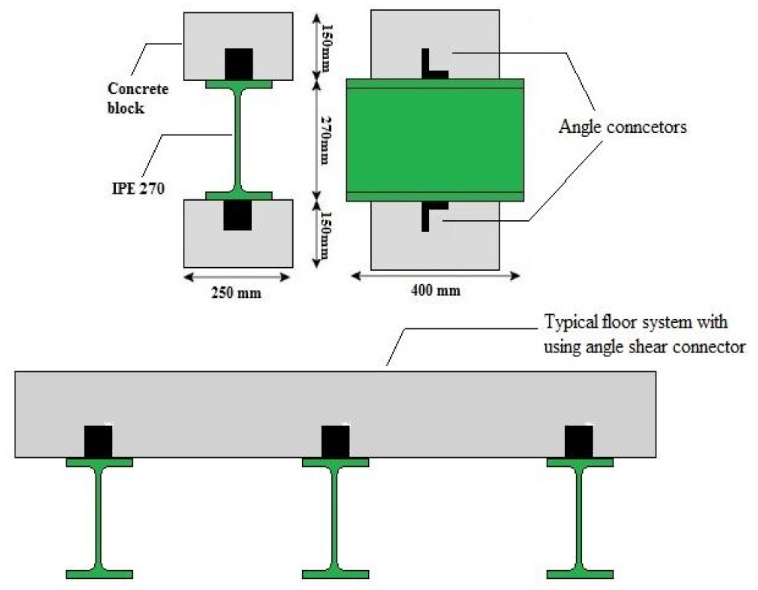
2.1. Statistical Data of Samples

In this study, the dataset was the information of experiments that eventually consisted of 584 test results (the specifications of the dataset are shown in Appendix A). The statistical properties of the whole dataset and input variables are indicated in

Table 1. Details of input variables.

Inputs	Variables	Min	Max	Mean Value	Std
Input 1	Slip (mm)	0.00	73.70	22.87	39.2
Input 2	Length (mm)	30.0	50.0	40.0	10.0
Input 3	Thickness (mm)	5.0	7.0	6.0	0.8
Input 4	Height (mm)	65.0	100.0	80.4	14.8
Input 5	Temperature (°C)	25.0	850.0	568.2	311.9
Input 6	Load (kN)	0.00	126.7	36.8	27.6
Outputs
Output 1	Slip (mm)	0.00	73.70	22.87	39.2
Output 2	Load (kN)	0.00	126.7	36.8	27.6

.

As shown in Table 1, the concrete’s compressive strength along with the steel properties remained at constant values with no involvement in the dataset. The database was set for variables such as the height, length and thickness of the shear connectors, which directly affect the split-tensile capacity of the composite floor system, especially at elevated temperatures. Load and slip could be replaced by each other in the placement order either as an input or an output.

2.2. Analytical Assessment

Recently, some research studies have been conducted on the performance of welded built-up steel members using AI techniques [25]. The following sections describe the architecture and some background of the employed algorithms in the current study.

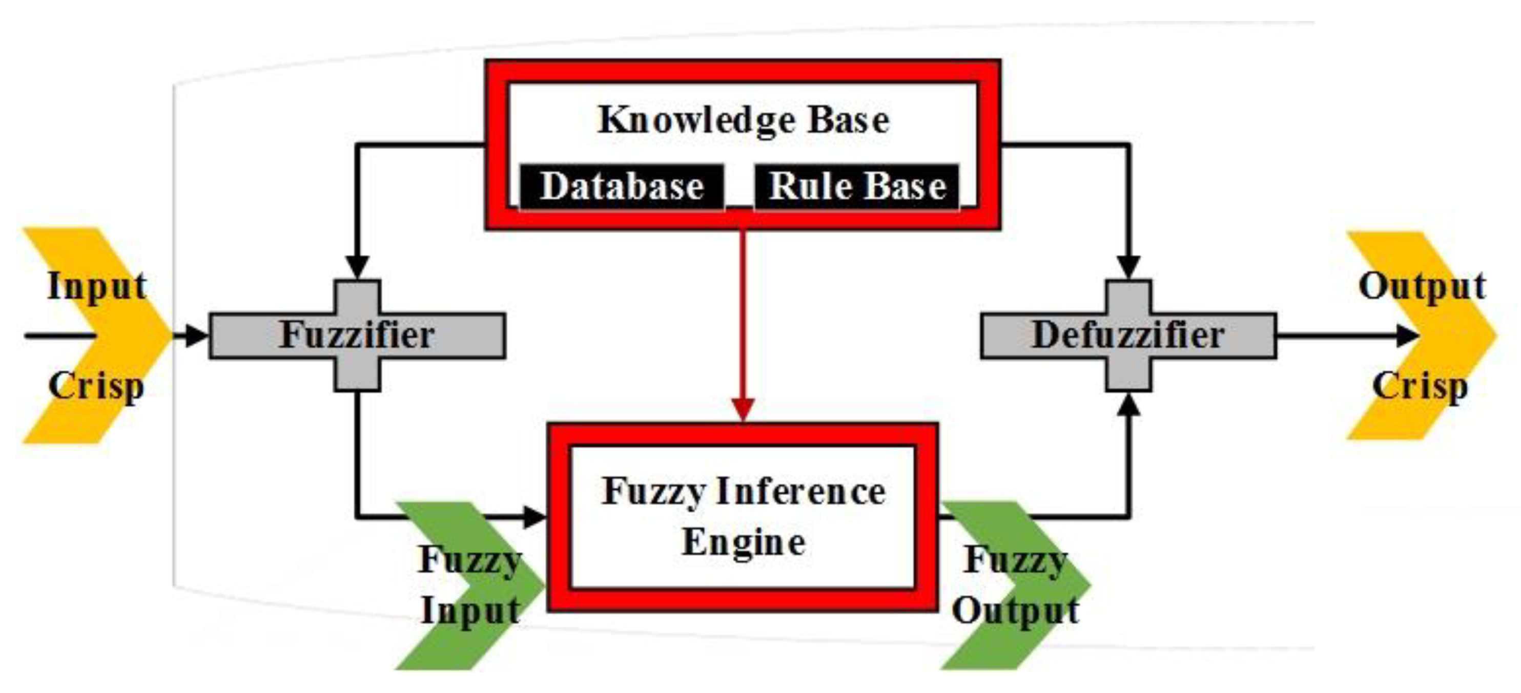
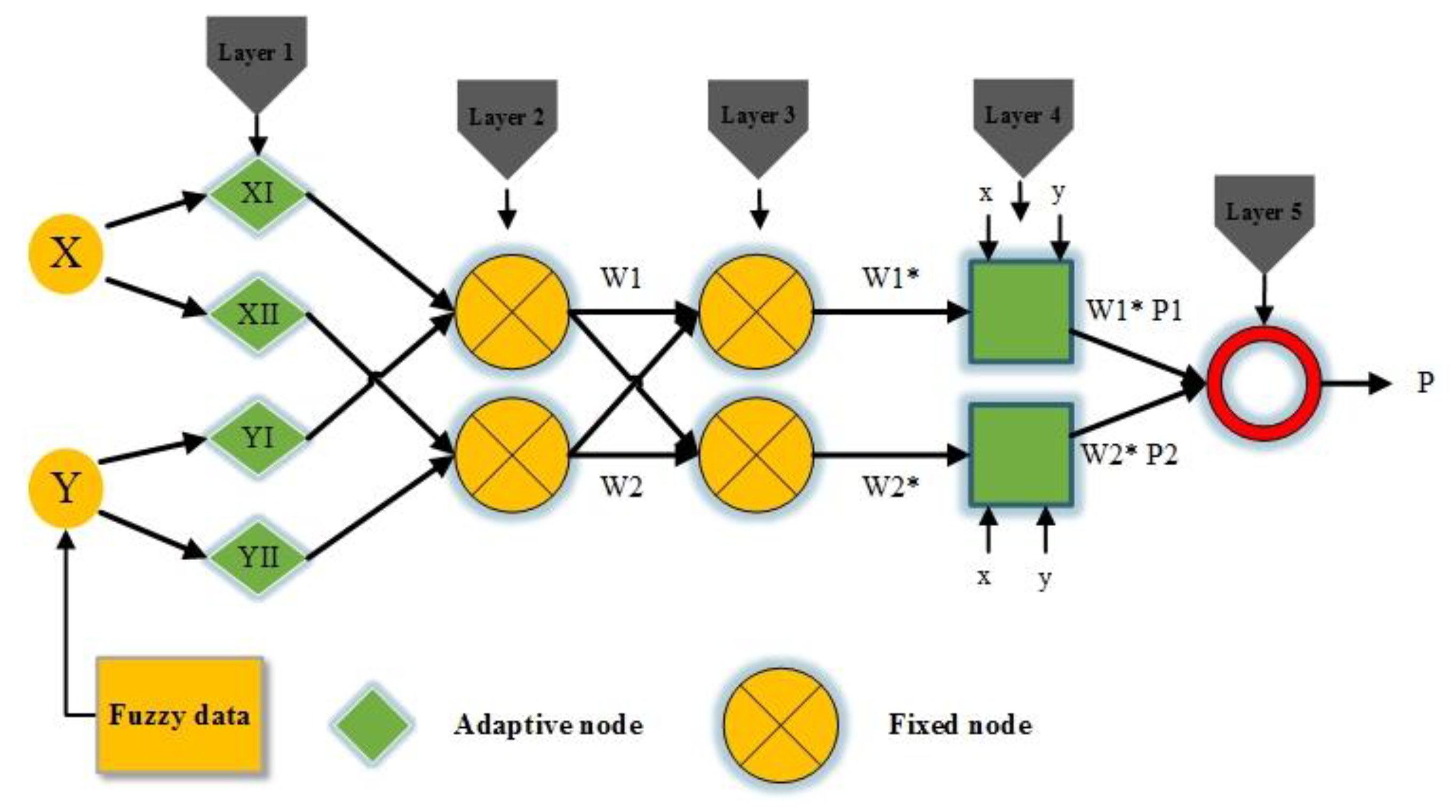
2.2.1. ANFIS Algorithm and Architecture

In an adaptive network (AN), nodes are directly connected by links, and every node acts in a defined performance on its receiving signals to produce a single node output; therefore, this procedure is made up of a multi-layer feed-forward system [34]. Notably, the configuration of an AN acts as a static node function on its receiving signals to produce a single node output, and every node performance is a parameterized function with changeable parameters. With any alteration of these parameters, the node functions are altered such as the overall behavior of the AN, Figure 2. In a fuzzy inference system (FIS), membership function parameters are tuned by a specific technique. Indeed, an ANFIS is utilized to delineate the optimal amounts of equivalent FIS parameters through a learning algorithm [44]. Across the training session(s), parameter optimization is performed in a way that the error between actual output and target decreases. A hybrid algorithm is utilized for the optimization that is a combination of gradient descent and the least square estimate method. The optimized parameters are called premise parameters that specify the shape of the membership functions (MFs). To minimize the error measure, each optimization routine could be used after the MFs are generated. The parameter set of the AN permits the fuzzy systems to learn from the modeling data.

The ANFIS network has five layers called the fuzzy layer, normalized layer, product layer, total output layer and de-fuzzy layer, as shown in Figure 3 [45]. During this technique, a threshold value between the output and the actual value is set and the following parameters are obtained by the least-squares model, while an error for all data is also received. If the threshold value exceeds the deliberated threshold, using the gradient descent method the premise parameters are updated. This continues until the error turns out to be less than the threshold. Because the parameters are simultaneously obtained by using two algorithms (the decent gradient and least-squares algorithms), the utilized algorithm during this procedure is called a hybrid algorithm.

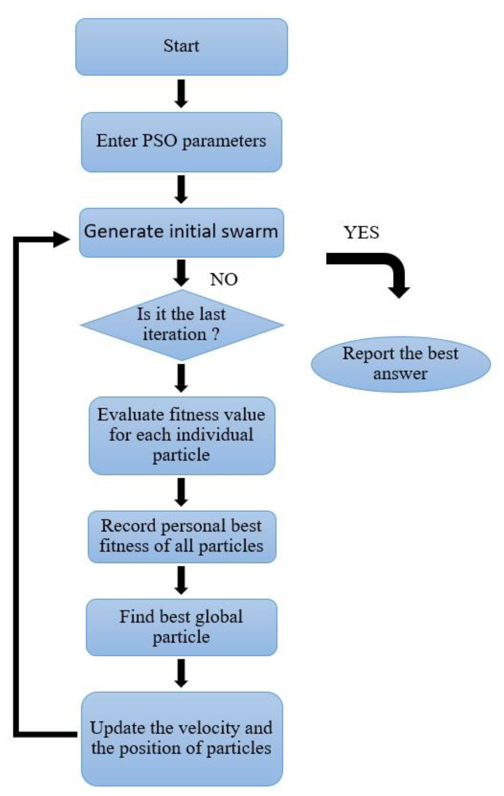
2.2.2. Particle Swarm Optimization (PSO)

The PSO algorithm is another member of the swarm intelligence algorithms initially generated by Kennedy and Eberhart [46] while sharing many aspects with evolutionary computation models such as GA. Similar to other population-based intelligence models, PSO needs an initial population of random resolutions. The search for optimal values is gained by updating the generations without evolution operators such as mutation and crossover. The potential decisions are generally called particles in PSO, flying through the resolution space by following their own experiences and the current optimal particles. Thus, the performance of PSO is comparable with GA and may be regarded as an alternative approach for GA. Figure 4 indicates the systematic sequences of the PSO algorithm.

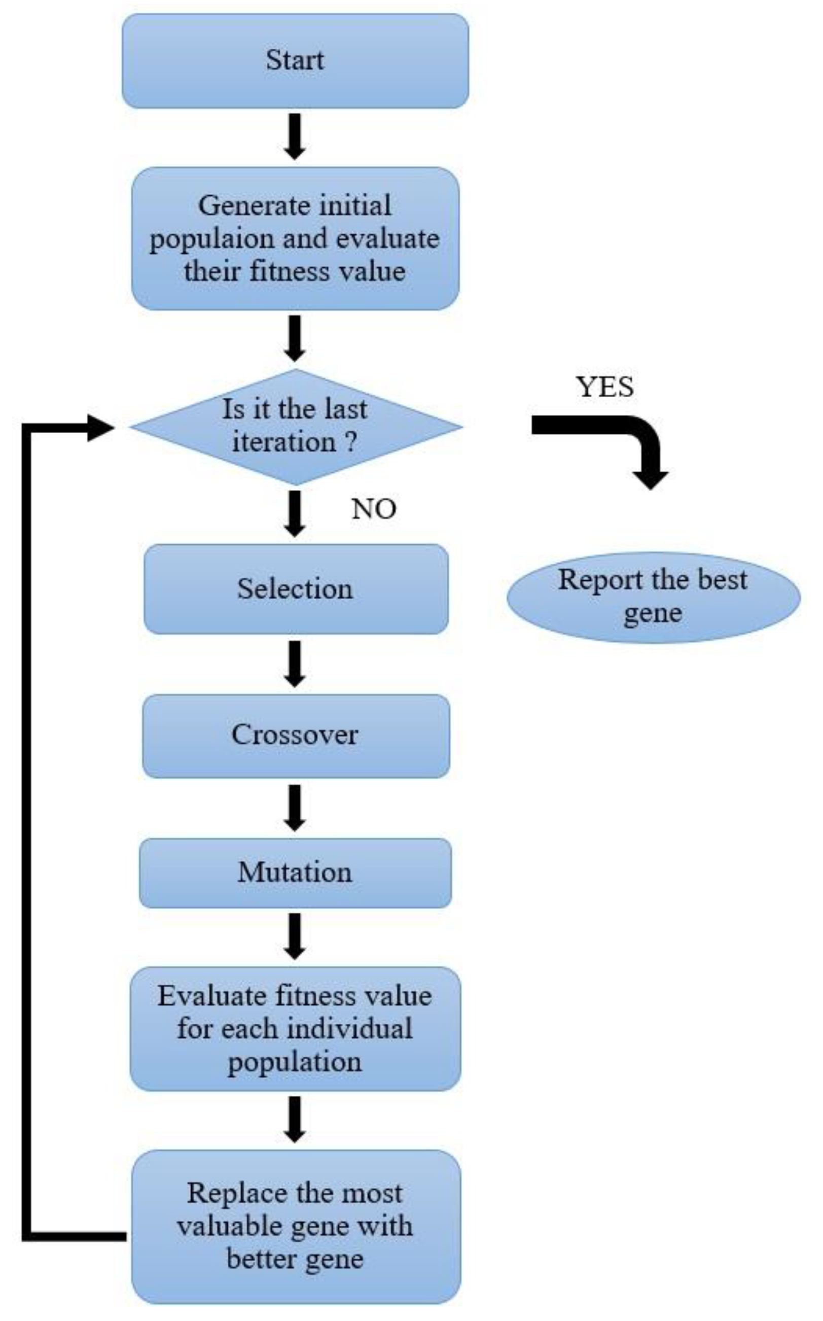
2.2.3. Genetic Algorithm (GA)

Holland (1992) [47] introduced the GA based on the extended evolution theory of Darwin that was developed by Goldberg and Holland (1988) [48]. As a member of the larger group of evolutionary algorithms (EAs), the GA is a metaheuristic algorithm based on the principles of biological evolution in nature. After many evolutions, the best individual is obtained. Compared with other optimizing methods, the GA includes good robustness and convergence. With the same accuracy of calculation, the GA takes the least time to find an optimal resolution [49]. Figure 5 represents the step-by-step platform of the GA algorithm.

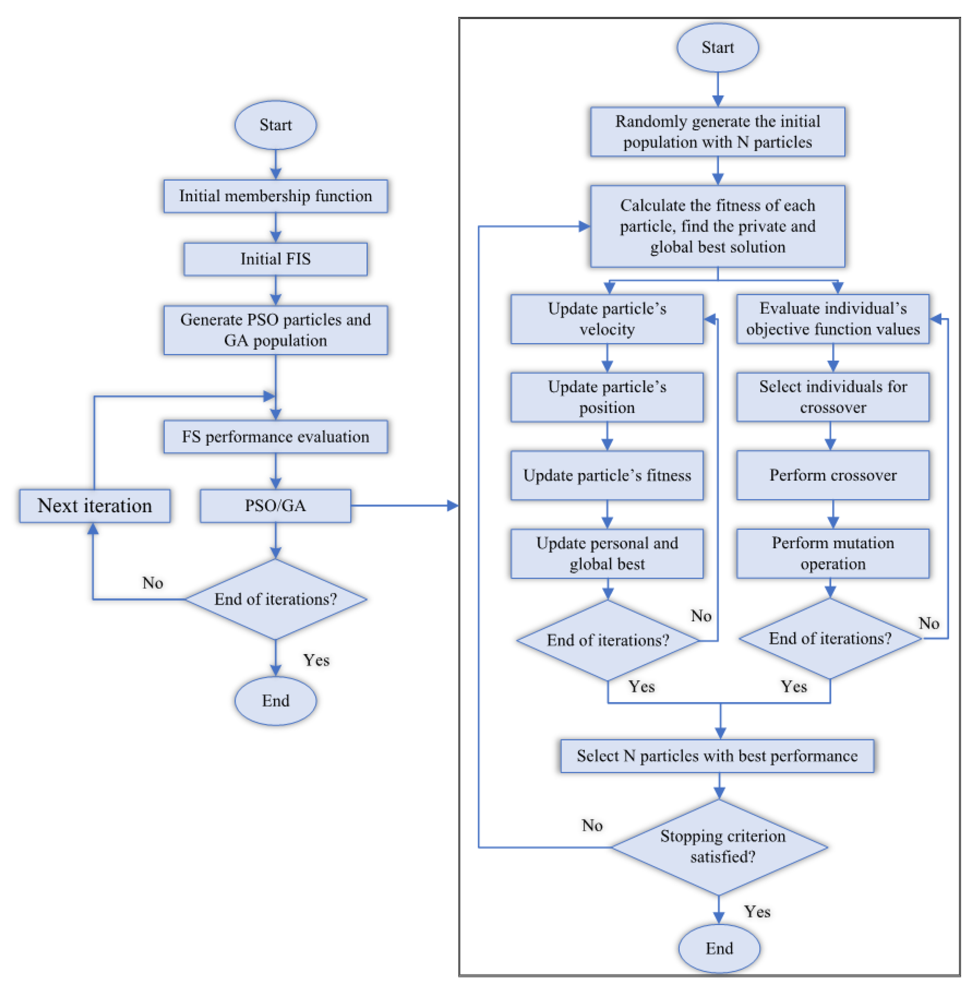
2.2.4. Hybrid ANPG Architecture

For the first time, a hybridized ANFIS using PSO and GA techniques was applied to solve a composite floor system problem. The combination of the sequential PSO-GA and ANFIS is depicted in Figure 6. In order to identify the best weights and to select suitable functions, the ANPG method was performed several times to predict one specific outcome with a variety of input scenarios. First, in PSO, swarm is initiated by a group of random resolutions as a particle, while showing the particle’s position. Then, the specific velocity is identified, the transmitting function is triggered, and the GA procedure initiates to optimize the final problem space. Finally, a particular velocity is gained for any ith particle in every cycle by using Equation (1) where w represents the inertia weight.

$$v_i\left(t+1\right)=w{v}_i\left(t\right)+c_1{\varphi }_1\left(p_i\left(t\right)-x_i\left(t\right)\right)+c_2{\varphi }_2\left(p_i\left(t\right)-x_i\left(t\right)\right)$$

(1)

$c_1$ and $c_2$ represent the positive acceleration coefficients. ${\overrightarrow{\varphi }}_1$ and ${\overrightarrow{\varphi }}_2$ show uniformly distributed random vectors [0, 1], in which a random value is tried for each dimension. ${\overrightarrow{v}}_i$ limited to $\left[-{\overrightarrow{v}}_{\max },{\overrightarrow{v}}_{\max }\right]$ series is reliant on the problem. In some cases, the velocity exceeds the mentioned curb and is rearranged within its suitable limits. Based on their velocities, every particle alters its position based on the following Equation (2):

$$s\left(t+1\right)=s\left(t\right)+v\left(t+1\right)$$

(2)

Based on ${\overrightarrow{v}}_i$ and ${\overrightarrow{s}}_i$, the particle population tends to cluster around the best number.

Figure 6. The sequential combination of the hybrid ANPG algorithm.

Figure 6. The sequential combination of the hybrid ANPG algorithm.

The ANPG hybrid method operates in regard to random population generation and is based on avian mass flight behavior modeling and simulation of fish mass movement. A global minimization method can deal with questions whose answers are a point or surface in n-dimensional space. A random population is assumed in this space, and an elementary velocity is defined for it and between the particles to the communication channels. The particles move through the response space, and the outcomes are computed on a “merit basis” after each time interval. Then, particles speed up toward the particles of higher competence that are in matching communication groups. Although each method is performed satisfactorily in a range of problems, it demonstrates pronounced capability in resolving continuous problems in optimization. The GA, by using evolutionary biology methods, tries to find the optimum formula for predicting or pattern matching. The GA could be an effective choice for regression-based prediction techniques, while its modeling is a programming technique based on genetic evolution to problem resolutions. The solved problem possesses inputs converted into solutions through a patterned process of genetic evolution. Afterward, by using the fitness function, the solutions are verified as candidates. The ANPG algorithm terminates in case the condition of problem exit is arranged. Generally, it is an iteration-based algorithm in which most of its parts are randomly selected.

2.2.5. Extreme Learning Machine (ELM)

As a single-layer learning tool, the ELM method was introduced which is similar to a feed-forward neural network [50]. In the ELM method, the output weights are analytically determined while the weights of input are defined randomly. The superiority of the ELM method is its extremely fast ability to find target weights. Additionally, without exterior interference, the ELM method is able to determine all the network parameters. In the case of prediction and characteristic estimation for concrete products, the ELM method is efficient and reliable [51] and because of these benefits it has gained high popularity and applicability.

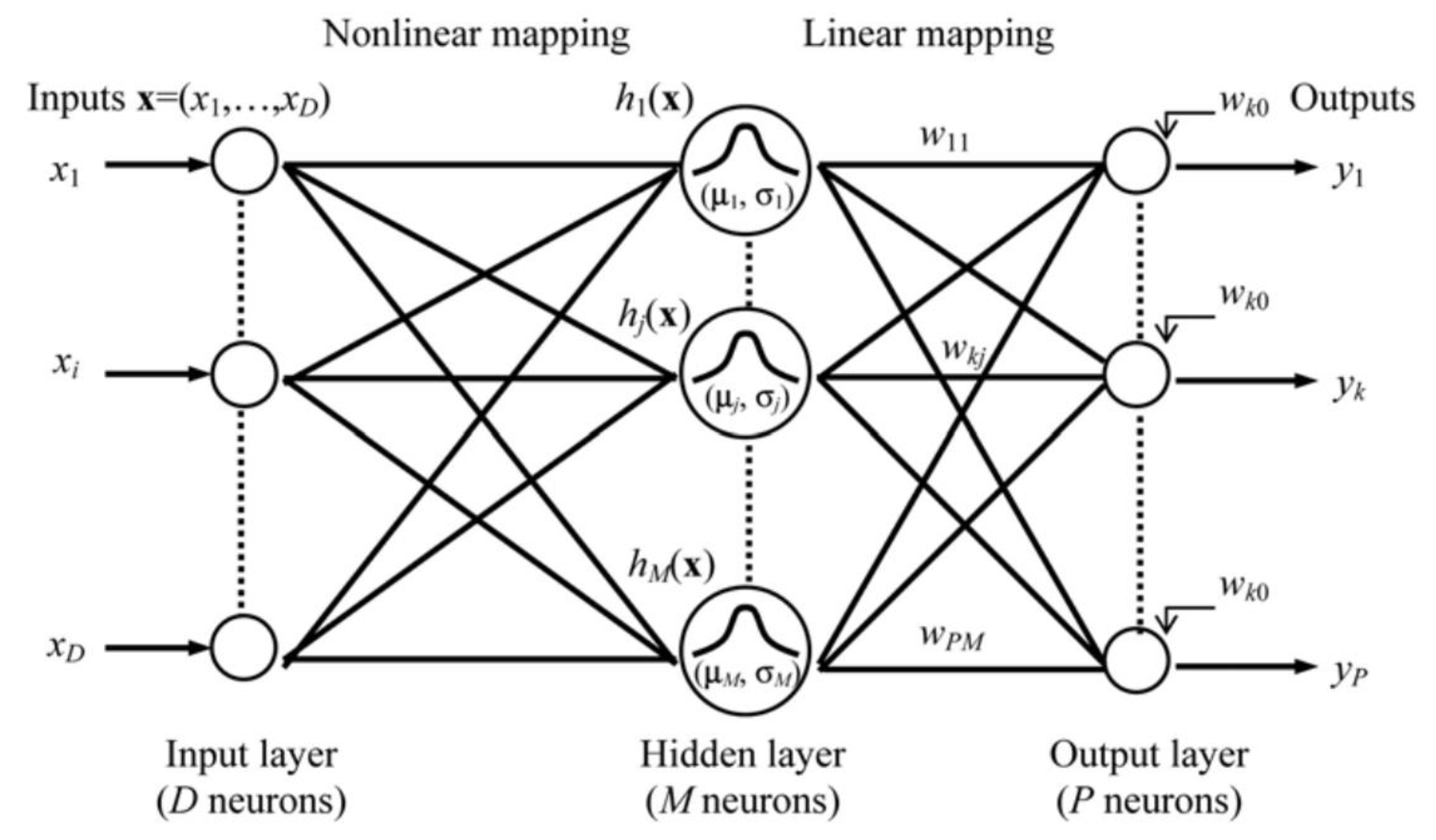
2.2.6. Radial Basis Function Network (RBFN) Method

Generally, in each RBFN architecture, a set of D-dimensional radial activation functions estimate the input function f_(x). The architecture consists of the D neuron input layer, the P neuron output layer and the M neuron hidden layer. The biases at each output neuron and adjustable weights between the hidden and output layers are shown in Figure 7 [52,53]. The system is represented by the nth input vector, and as described in Equation (3), the approximation function f_(x) can be represented as a linear combination of radial basis functions in which the output of the kth network consists of the sum of weighted hidden layer neurons plus the bias [41]:

$$\hat{f}\left(X\right)=wh\left(X\right)+w,\hspace{1em}k=1,2,\dots ,P$$

(3)

where:

• w_kj = weight of the jth basis function and kth output;
• h_j (Xⁿ) = output of jth hidden neuron for the input vector (xⁿ);
• w_(k0) = bias term at kth output neuron.

Figure 7. The architecture of the RBF network.

Figure 7. The architecture of the RBF network.

2.2.7. Performance Evaluation

Models of all the developed methods were evaluated by using evaluation criteria namely, root mean squared error (RMSE), determination coefficient (R²) and Pearson correlation coefficient (r) as follows:

$$RMSE=\sqrt{\frac{{\displaystyle \sum _{i=1}^n{(P_i-O_i)}^2}}{n}}$$

(4)

$$\mathrm{r}=\frac{\mathrm{n}\left({\displaystyle \sum _{\mathrm{i}=1}^{\mathrm{n}}{\mathrm{O}}_{\mathrm{i}}·{\mathrm{P}}_{\mathrm{i}}}\right)-\left({\displaystyle \sum _{\mathrm{i}=1}^{\mathrm{n}}{\mathrm{O}}_{\mathrm{i}}}\right)·\left({\displaystyle \sum _{\mathrm{i}=1}^{\mathrm{n}}{\mathrm{P}}_{\mathrm{i}}}\right)}{\sqrt{\left(\mathrm{n}{\displaystyle \sum _{\mathrm{i}=1}^{\mathrm{n}}{\mathrm{O}}_{\mathrm{i}}^2}-{\left({\displaystyle \sum _{\mathrm{i}=1}^{\mathrm{n}}{\mathrm{O}}_{\mathrm{i}}}\right)}^2\right)·\left(\mathrm{n}{\displaystyle \sum _{\mathrm{i}=1}^{\mathrm{n}}{\mathrm{P}}_{\mathrm{i}}{}^2}-{\left({\displaystyle \sum _{\mathrm{i}=1}^{\mathrm{n}}{\mathrm{P}}_{\mathrm{i}}}\right)}^2\right)}}$$

(5)

$${\mathrm{R}}^2=\frac{{\left[{\displaystyle \sum _{\mathrm{i}=1}^{\mathrm{n}}\left({\mathrm{O}}_{\mathrm{i}}-\overline{{\mathrm{O}}_{\mathrm{i}}}\right)·\left({\mathrm{P}}_{\mathrm{i}}-\overline{{\mathrm{P}}_{\mathrm{i}}}\right)}\right]}^2}{{\displaystyle \sum _{\mathrm{i}=1}^{\mathrm{n}}\left({\mathrm{O}}_{\mathrm{i}}-\overline{{\mathrm{O}}_{\mathrm{i}}}\right)·{\displaystyle \sum _{\mathrm{i}=1}^{\mathrm{n}}\left({\mathrm{P}}_{\mathrm{i}}-\overline{{\mathrm{P}}_{\mathrm{i}}}\right)}}}$$

(6)

where $P_i$ and $O_i$ are the predicted and observed variables, and n is the total number of considered data. Alternatively, MATLAB (2019) was used to compare the code performance of the ANPG, RBFN and ELM methods in one computer system with no external compiler or toolbox implementation.

3. Results

In this study, the employed algorithms (the ANPG, RBFN and ELM methods) were separately tuned. To optimize the coefficients of specific parameters for each algorithm, the other parameters were considered to remain constant. By changing the coefficient value, the best value was determined and used for different parameters. Therefore, all the algorithms were repeatedly used and revised to develop the algorithms, as explained below.

3.1. ANFIS-PSO-GA (ANPG) Method

The parameters of the ANPG method were adjusted and are summarized in

Table 2. Parameter characteristics used for the ANPG method.

FIS Clusters	Population Size	PSO-Iterations	GA-Sub-Iteration	MAX-Iteration	Inertia Weight	Damping Ratio	Learning Coefficient		Conducted Fuzzy Function
							Personal	Global
10	90	50	45	150	1.00	0.988	1	2	bell-shaped

. The inputs of the dataset were initially defined and predicted, while the predition values of split-tensile load and slip were obtained separately in different analyses (Table 2). The results of the regression and comparative graphs are shown in Figure 8 and Figure 9, respectively. As shown in Figure 8 and

Table 3. Output and input database.

Split-tensile load prediction		Test	Train
	Std *	3.869	3.1884
	emean	−0.014	−0.081
	R2	0.925	0.946
	r	0.962	0.973
	RMSE	3.869	4.868
Slip prediction		Test	Train
	Std *	0.954	1.136
	emean	−0.012	−0.049
	R2	0.961	0.953
	r	0.980	0.976
	RMSE	0.962	1.736

* Std, standard deviation.

, the ANPG method is more successful for predicting values of slip than for predicting tensile load, which could be due to the properties of this type of NN or simply to the output being more predictable. In addition, the test results of slip and load prediction demonstrate good consistency with the training results, indicating the reliability of this method for predicting complex and nonlinear test results. Despite the acceptability of the outputs of the other employed ELM method, the inconsistent test and training results reduced the reliability of the output(s).

For the tensile load, the standard deviation of the two test and training phases is 18%, and the standard deviation is 16% for slip value outputs, indicating less error concentration in the first output than the second output, Figure 10.

3.2. RBFN

Table 4. The parameter characteristics used for the RBFN method.

FIS Clusters	Population Size	MAX-Iteration	Cross over Percentage	Mutation Percentage	Mutation Rate	Selection Pressure
10	180	200	1.00	0.5	0.1	8

shows the settings used for the combination of a hybrid grid. The results of the RBFN method are presented in

Table 5. Analytical prediction results through the RBFN method.

Split-tensile load prediction		Test	Train
	Std *	3.950	3.003
	emean	−0.119	2.75 × 10−5
	R2	0.946	0.959
	r	0.972	0.979
	RMSE	3.949	4.585
Slip prediction		Test	Train
	Std *	1.556	1.330
	emean	−0.155	−0.036
	R2	0.906	0.948
	r	0.952	0.973
	RMSE	1.562	2.033

* Std, standard deviation.

and Figure 11 and Figure 12. In this method, the results for the lateral load output were much better than the compressive strength. In addition, the test and training phase results for the first output were very similar.

The results of this neural network approximation for the tensile e-load value output indicated more concentration at the boundary. In particular, during the training phase, the reliable evaluation criteria results are approximate. Another point to note from the graphs in Figure 12 is the relatively low error for tensile-load data below 5 MPa for both the training and test phases and relatively high error for data above 20 MPa, especially during the training phase (Figure 12). Furthermore, slip value outputs indicate higher irregularities above 10 mm. The standard deviation of the test and training phases for the tensile load is 24% and the standard deviation is 15% for slip value outputs, indicating a better concentration of errors in slip output than load output (Figure 13).

3.3. ELM Method

The last neural network is the ELM method and the settings and are summarized in

Table 6. The parameter characteristics used for the ELM method.

FIS Clusters	Regression	Hidden Neurons	Activation Function
1.0	0.008	845	Hard Limited

. The results are also acceptable for both outputs, as shown in Figure 14 and Figure 15. However, by comparing the load output evaluation criteria to those of the slip value outputs and by comparing the test and training results, the load outputs show more consistency. At the same time, it is different for other products, as shown in

Table 7. Analytical prediction results through the ELM algorithm.

Split-tensile load prediction		Test	Train
	Std *	4.341	3.949
	emean	0.128	0.022
	R2	0.906	0.932
	r	0.9522	0.965
	RMSE	4.339	6.030
Slip prediction		Test	Train
	Std *	1.454	1.851
	emean	−0.086	0.044
	R2	0.923	0.922
	r	0.961	0.960
	RMSE	1.455	2.827

* Std, standard deviation.

.

Regarding the standard deviation and error histogram in Figure 16, errors have a greater focus on slip value outputs which make the outputs more reliable. The tensile-load outputs presented are probably good results; however, due to the lack of focus on the errors of the center axis, an unprecedented response could be high with unacceptable errors.

4. Discussion

To define the inputs of RMSE, R² and r, an ANFIS was individually trained for every input. The effect of every input on the output could be delineated based on the determined analytical parameters for any input. Inputs with the smallest training RMSE had the most effect or relevance to the output. To identify the overfitting between test data and training, RMSE testing was applied. If the testing RMSE is very high, the regression of data is not beneficial. According to the RMSE training, the optimum combination is PSO and the GA with an ANFIS, with the most substantial accuracy on the output evaluation parameters. By examining the results of all methods, it is concluded that both split-tensile load and slip value outputs indicate a likely predictable trend due to the described inputs and useful employed NNs. A comparison of the best results for each method is shown in Figure 17, where the RBFN prediction is stronger compared to the others with R² (test) = 0.9466, R² (train) = 0.9591; r (test) = 0.973, r (train) = 0.973; and RMSE (test) = 3.949, RMSE (train) = 4.585. By evaluating the test phase error histograms shown in Figure 10, Figure 13 and Figure 16, due to the minor error interval in the ANPG method, the three graphs show reasonable concentration around the center, and the chance of obtaining a high error response is relatively low compared to the other methods. From the normal distribution point of view in each rectangular histogram of error, 68% of the data are within one time of the standard deviation of the mean value, 95% of the data are within two times of the standard deviation, and 99.7% of the data are within three times of the standard deviation [54,55,56]. Based on the results and discussion, all of the represented histograms in this paper are in agreement with the mentioned fact. Nevertheless, the charts (load error histograms) are consistent with the normal distribution paradigm, but according to Table 3, Table 4 and Table 5, different standard deviations and mean values lead to different shapes of the bell curves of load charts compared to the slip charts.

For slip value output, the ANPG method also provides the best result, as shown in Figure 18. The evaluation of the test phase for the ANPG method is R² (test) = 0.961, R² (train) = 0.952; r (test) = 0.980, r (train) = 0.976; and RMSE (test) = 0.962, RMSE (train) = 1.735. Thus, in the test phase, the result presented by the ANPG method is more acceptable.

The calculated equations from the linear regressions are summarized in

Table 8. The calculated tensile-load regression equation of the implemented models.

Model	Network Result
	Train Phase	Test Phase
	Regression Equation	Regression Equation
ANPG	y = 1.015x − 1.0466	y = 1.0018x − 0.0942
RBF	y = 0.8965x + 3.5193 *	y = 1.0x − 0.0015 **
ELM	y = 0.9403x + 2.6086	y = 0.8777x − 4.5728

* and ** are the best-achieved equations.

and

Table 9. The calculated slip value regression equation of the implemented models.

Model	Network Result
	Train Phase	Test Phase
	Regression Equation	Regression Equation
ANPG	y = 0.9405x − 0.0318 *	y = 0.9916x − 0.2411 **
RBF	y = 0.9491x − 0.1464	y = 1.0094x − 0.2069
ELM	y = 1.0421x − 0.6809	y = 0.802x − 1.624

* and ** are the best-achieved equations.

where the most decisive equations for both split-tensile load and slip value output of specific steel-concrete specimens manufactured by angle shear connector are highlighted.

5. Conclusions

In this study, a comparative AI study was conducted to identify the most susceptible structural characteristics of a composite floor system at elevated temperatures and to predict critical strength factors such as failure load and slip value of shear connectors. The main algorithm was a hybridized ANFIS technique with PSO and a GA called the ANPG method. The RBFN and ELM methods were also employed as subsidiary evaluation methods. In addition, this study utilized data from 584 test results which included width (mm), height (mm), thickness (mm), shear load (kN), temperature stages (°C) and slip value (mm). The major findings are as follows:

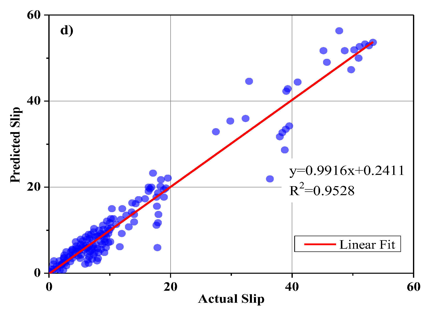
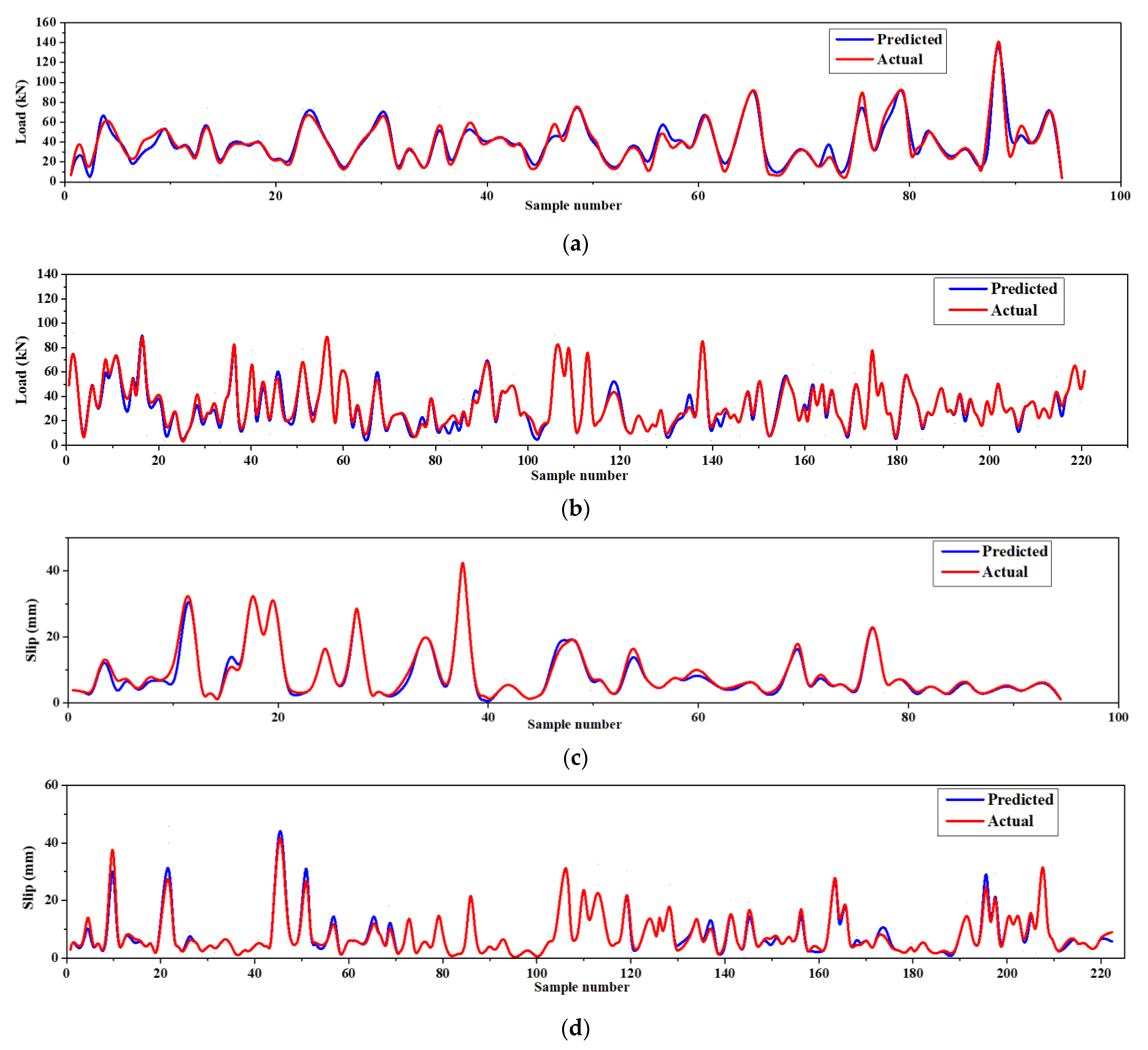
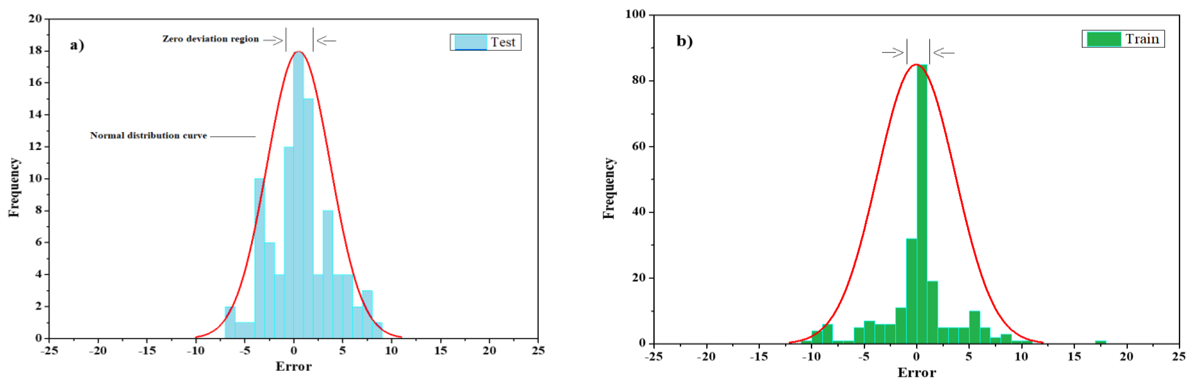
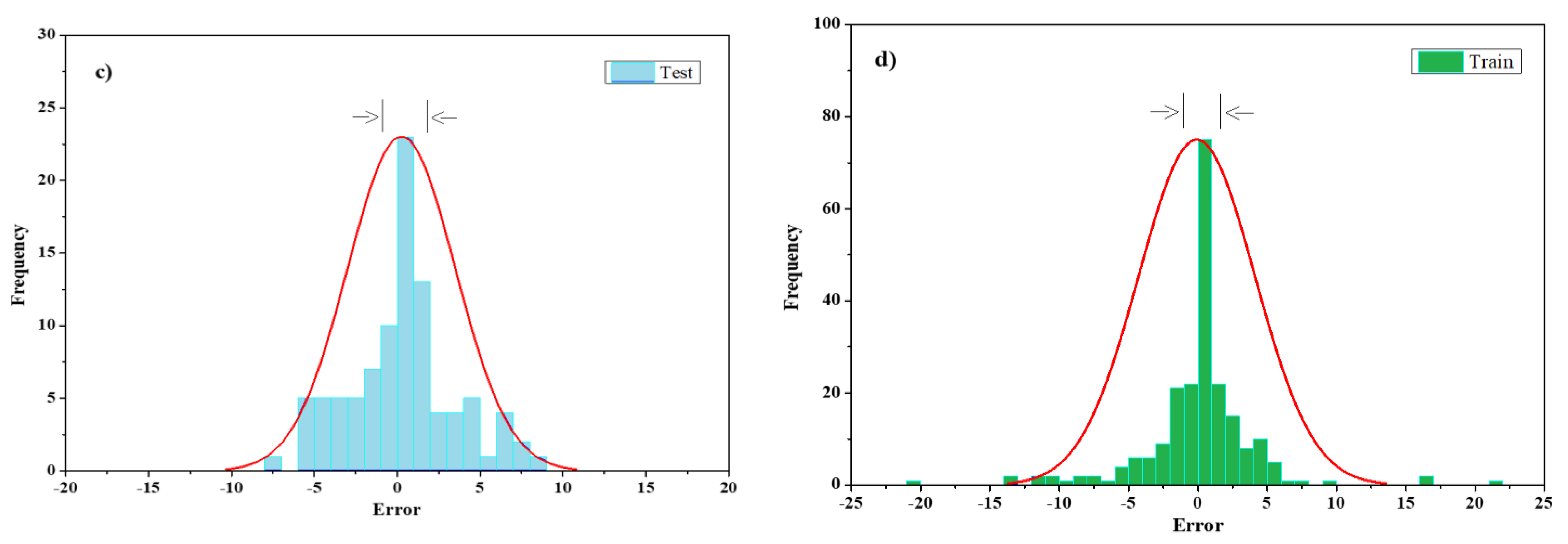
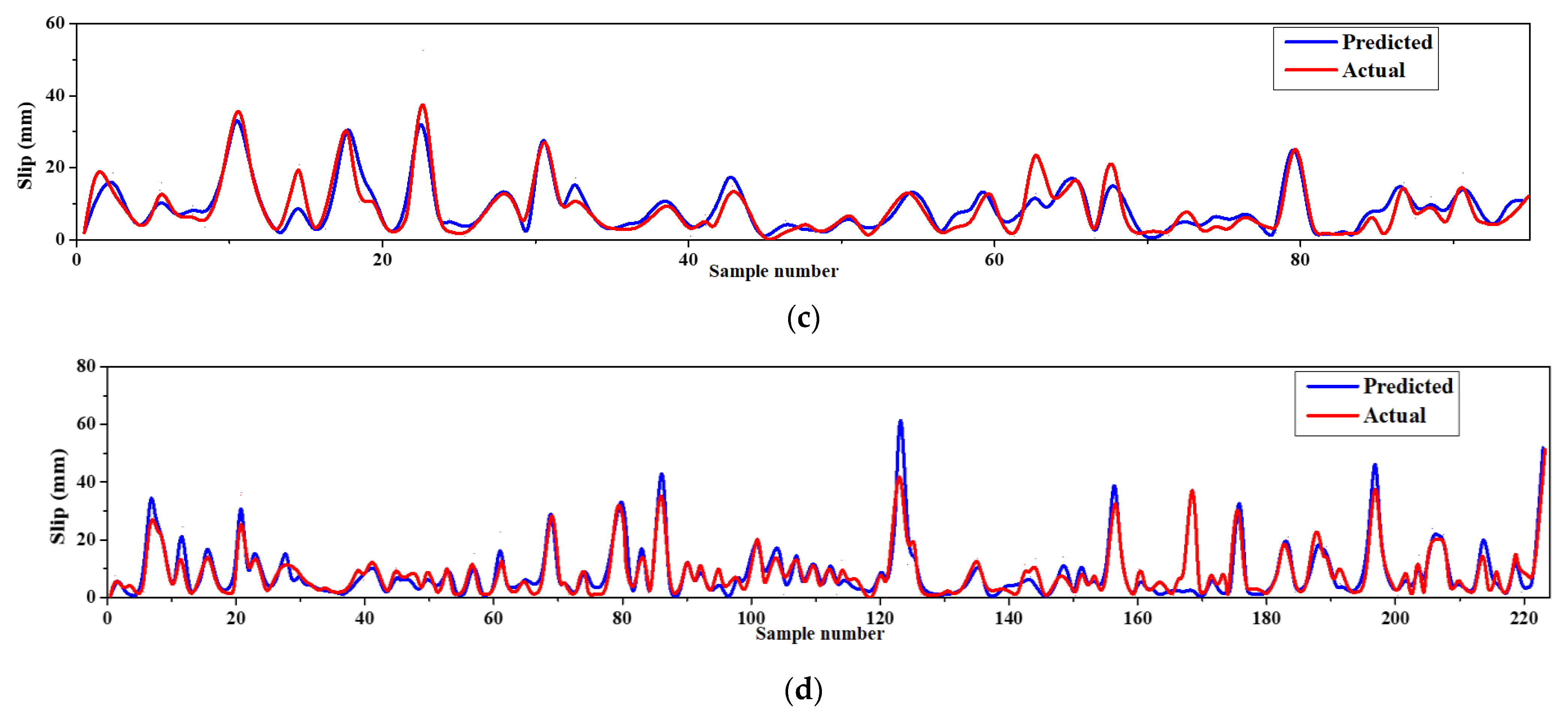
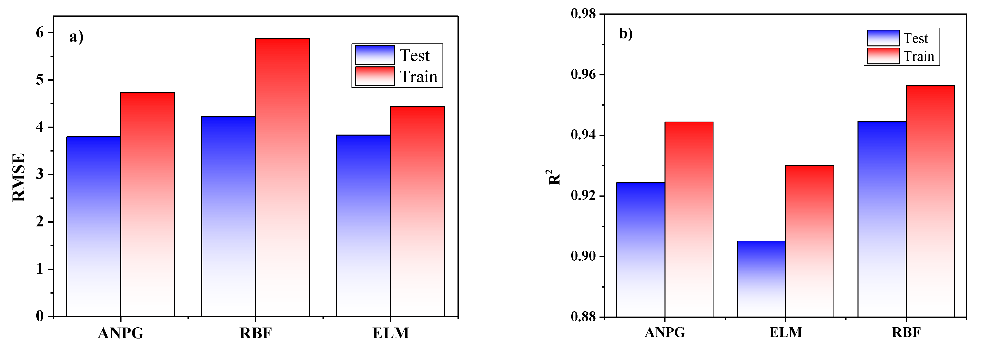
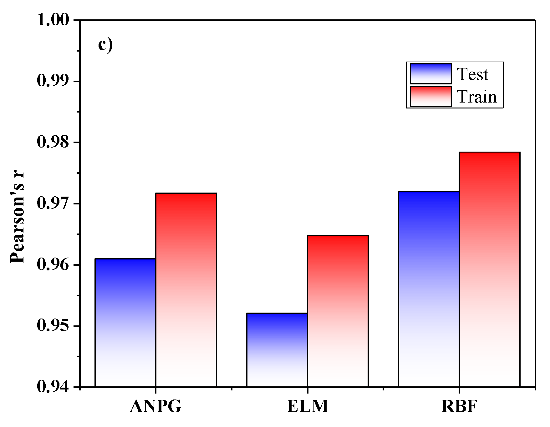
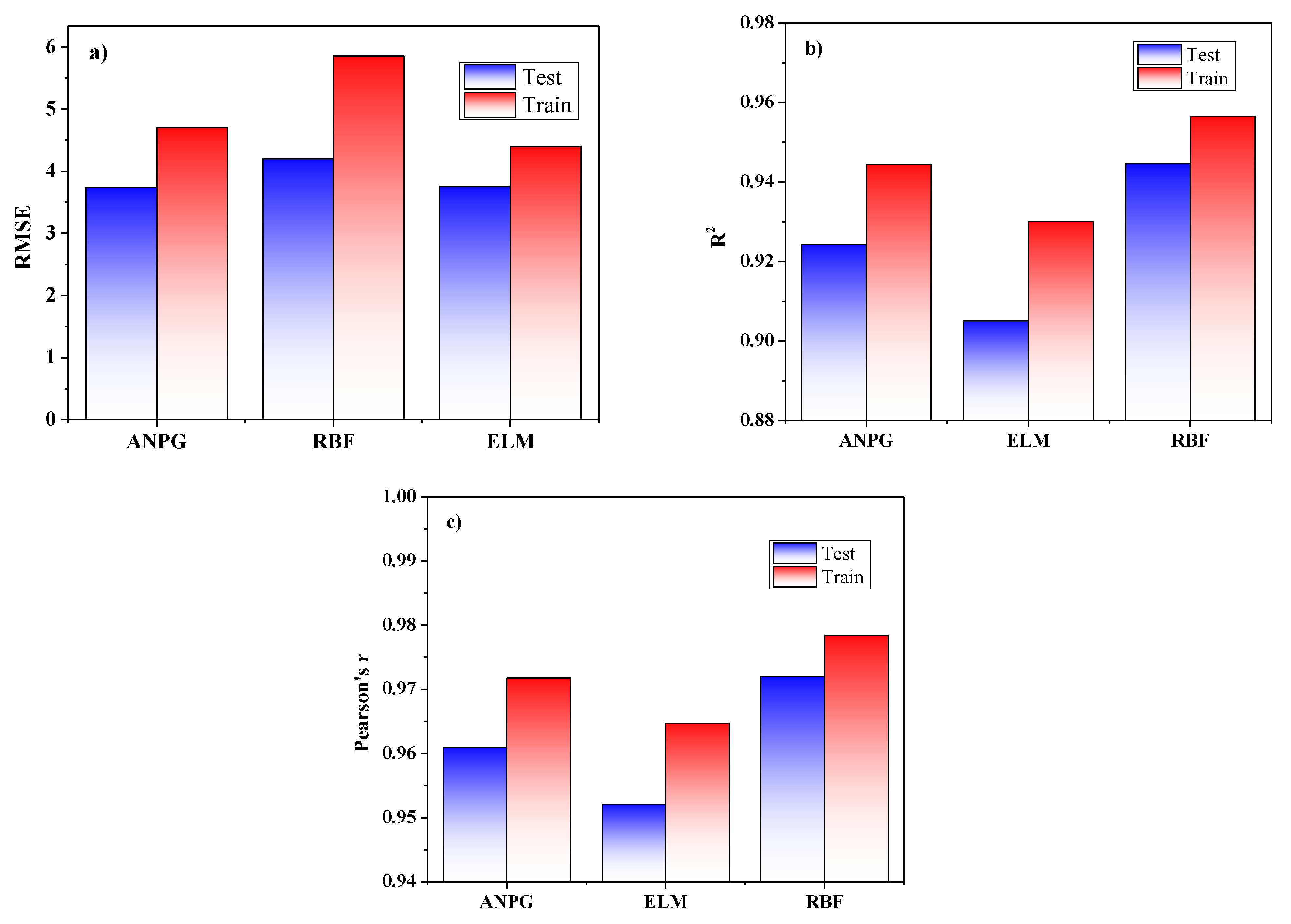
• Based on the results for slip value output, the ANPG method provided the best result. In this method, the test and training phase evaluation criteria were R² (test) = 0.961, R² (train) = 0.952; r (test) = 0.980, r (train) = 0.976; and RMSE (test) = 0.962, RMSE (train) = 1.736. Based on the tolerance charts, the test and training phases both represented suitable compatibility, while envelope curves dramatically maintained the same tolerance. According to the error histograms, the normal distribution shapes confirmed appropriate deviation from the mean value, and slip predictions had the least error value among other predictions.
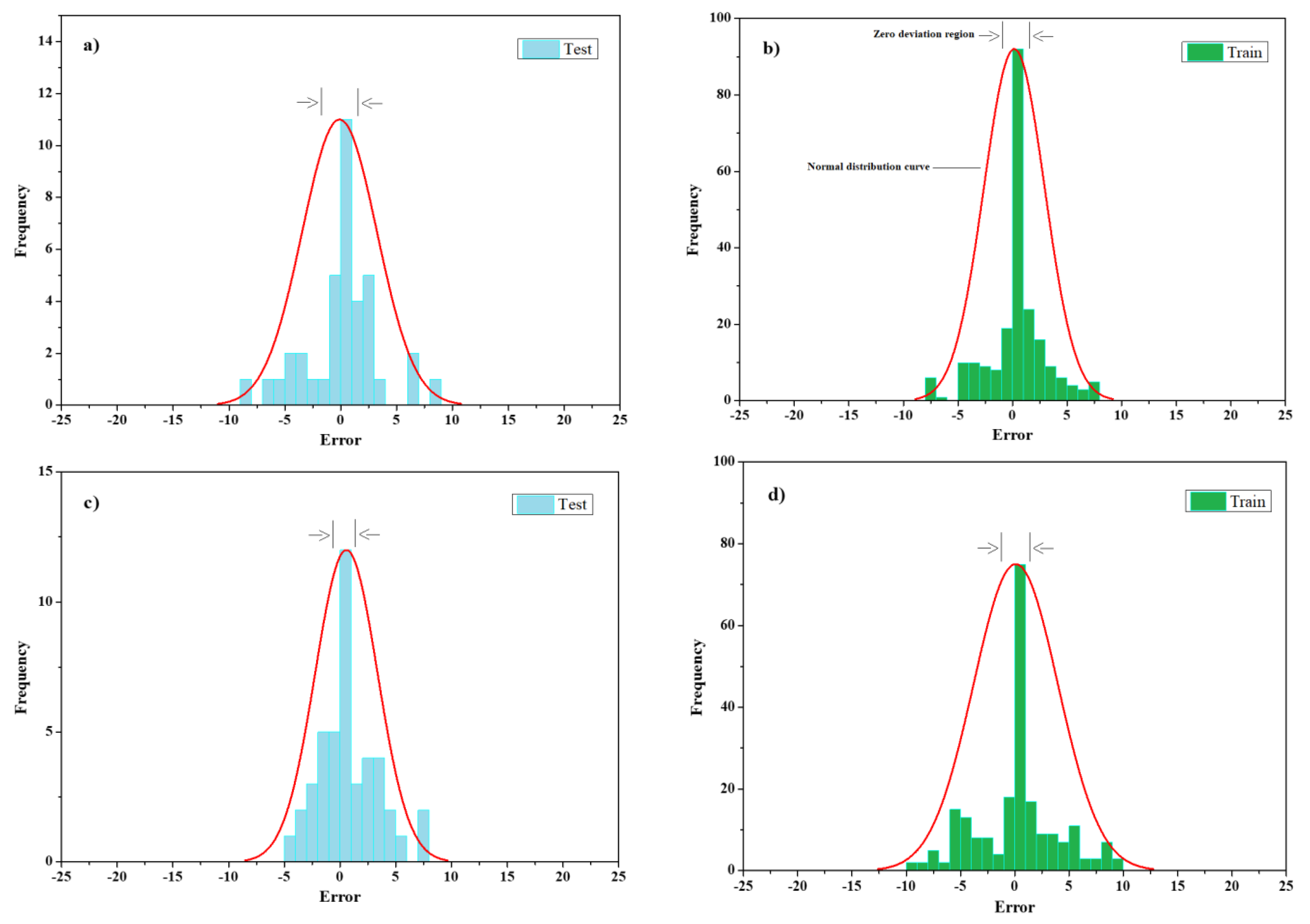
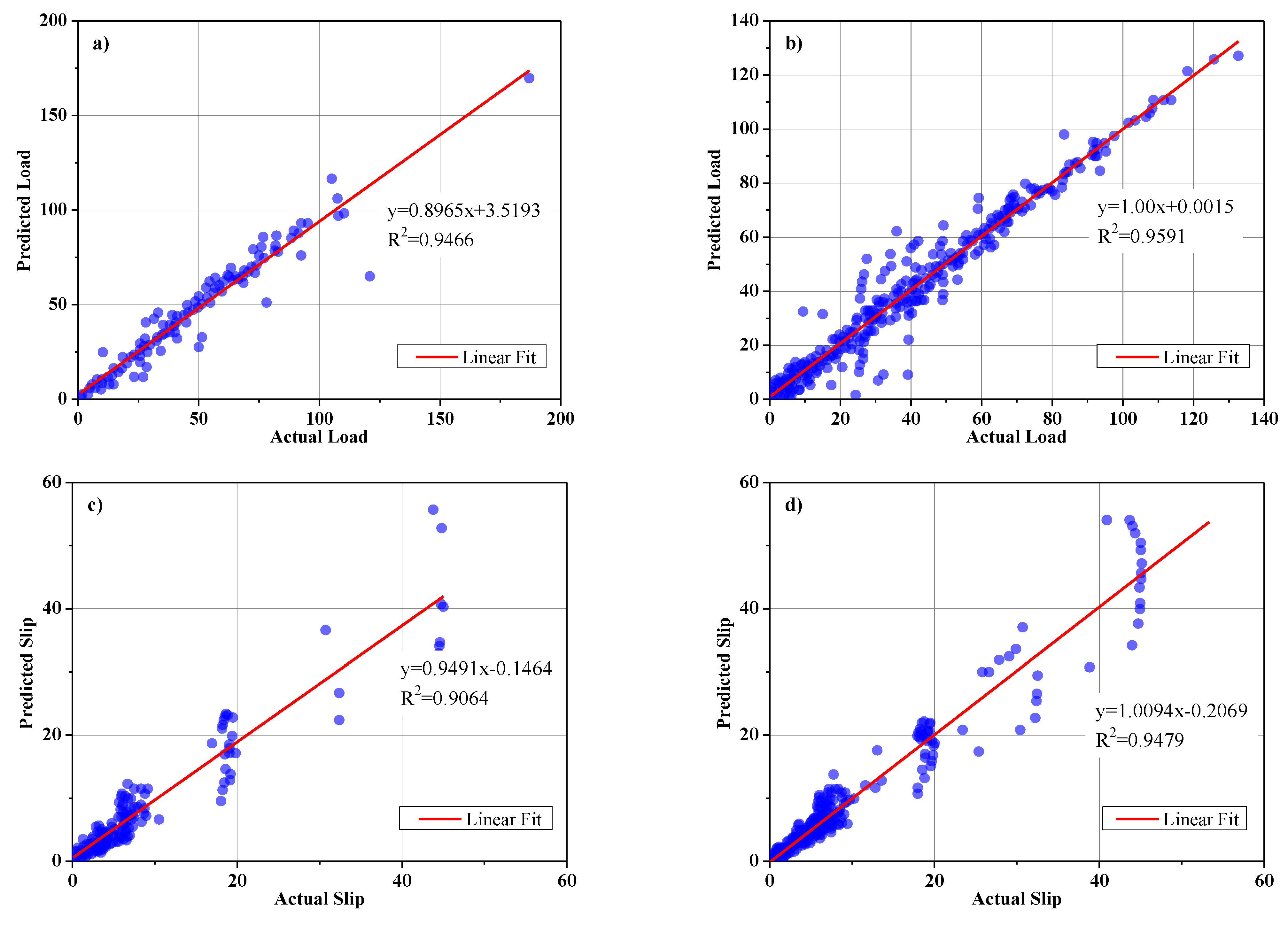
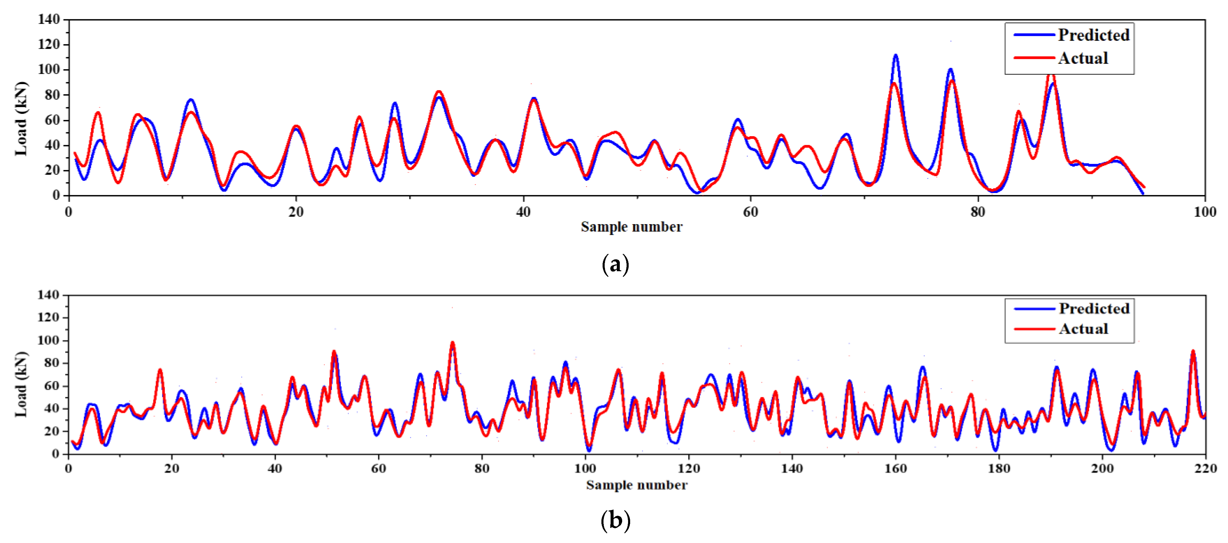
• In general, the RBFN method is an iteration-based algorithm in which most parts are randomly selected. For tensile-load output, the best result was obtained using the RBFN method with the performance parameters of R² (test) = 0.946, R² (train) = 0.959; r (test) = 0.973, r (train) = 0.973; and RMSE (test) = 3.949, RMSE (train) = 4.585. Tolerance curves in the load section illustrated the best coverage, and error histograms showed the least value in load prediction.
• The ELM method recorded the most suitable results in training phases for slip and split-tensile load prediction. In addition, the ELM method represented the lowest sensitivity against parameter contractions and performed a stable paradigm. For load, the results were R² (test) = 0.906, R² (train) = 0.932; r (test) = 0.952, r (train) = 0.965; and RMSE (test) = 4.339, RMSE (train) = 6.030. Furthermore, the slip results were R² (test) = 0.923, R² (train) = 0.922; r (test) = 0.961, r (train) = 0.960; RMSE (test) = 1.455, RMSE (train) = 2.877.
• For the identification study to determine the most critical factors on the shear-bearing capacity of a composite floor system at elevated temperatures, the ANPG method was performed on two subdata models, where slip and temperature were selected as the most significant parameters on the quality of the shear-bearing capacity. Based on the results, it could also be concluded that by restricting slip, the shear-bearing capacity could be improved at elevated temperatures, and conversely.

Finally, although all three methods (ELM, ANPG and RBFN) resulted in satisfactory prediction results, the ANPG method provided the best slip prediction results and the RBFN method achieved better load prediction results; nevertheless, all the above-mentioned methods are suitable for load and slip prediction.

References

- Utsab Katwal, T.A.; Tao, Z.; Uy, B.; Rahme, D. Tests of circular geopolymer concrete-filled steel columns under ambient and fire conditions. J. Constr. Steel Res. 2022, 196, 107393. [Google Scholar] [CrossRef]
- Xia, Y.; Shi, M.; Zhang, C.; Wang, C.; Sang, X.; Liu, R.; Zhao, P.; An, G.; Fang, H. Analysis of flexural failure mechanism of ultraviolet cured-in-place-pipe materials for buried pipelines rehabilitation based on curing temperature monitoring. Eng. Fail. Anal. 2022, 142, 106763. [Google Scholar] [CrossRef]
- Liu, K.; Yang, Z.; Wei, W.; Gao, B.; Xin, D.; Sun, C.; Gao, G.; Wu, G. Novel Detection Approach for Thermal Defects: Study on Its Feasibility and Application to Vehicle Cables. High Volt. 2022. [Google Scholar] [CrossRef]
- Huang, H.; Yao, Y.; Liang, C.; Ye, Y. Experimental study on cyclic performance of steel-hollow core partially encased composite spliced frame beam. Soil Dyn. Earthq. Eng. 2022, 163, 107499. [Google Scholar] [CrossRef]
- Zhang, Z.; Yang, Q.; Yu, Z.; Wang, H.; Zhang, T. Influence of Y2O3 addition on the microstructure of TiC reinforced Ti-based composite coating prepared by laser cladding. Mater. Charact. 2022, 189, 111962. [Google Scholar] [CrossRef]
- Zhang, C.; Abedini, M. Development of PI model for FRP composite retrofitted RC columns subjected to high strain rate loads using LBE function. Eng. Struct. 2022, 252, 113580. [Google Scholar] [CrossRef]
- Zhao, G.; Shi, L.; Yang, G.; Zhuang, X.; Cheng, B. 3D fibrous aerogels from 1D polymer nanofibers for energy and environmental applications. J. Mater. Chem. A 2023. [Google Scholar] [CrossRef]
- Li, J.; Chen, M.; Li, Z. Improved soil–structure interaction model considering time-lag effect. Comput. Geotech. 2022, 148, 104835. [Google Scholar] [CrossRef]
- Deng, E.-F.; Zhang, Z.; Zhang, C.-X.; Tang, Y.; Wang, W.; Du, Z.-J.; Gao, J.-P. Experimental study on flexural behavior of UHPC wet joint in prefabricated multi-girder bridge. Eng. Struct. 2023, 275, 115314. [Google Scholar] [CrossRef]
- Tian, L.-m.; Li, M.-h.; Li, L.; Li, D.-y.; Bai, C. Novel joint for improving the collapse resistance of steel frame structures in column-loss scenarios. Thin-Walled Struct. 2023, 182, 110219. [Google Scholar] [CrossRef]
- AzariJafari, H.; Amiri, M.J.T.; Ashrafian, A.; Rasekh, H.; Barforooshi, M.J.; Berenjian, J. Ternary blended cement: An eco-friendly alternative to improve resistivity of high-performance self-consolidating concrete against elevated temperature. J. Clean. Prod. 2019, 223, 575–586. [Google Scholar] [CrossRef]
- Toghroli, A.; Mehrabi, P.; Shariati, M.; Trung, N.T.; Jahandari, S.; Rasekh, H. Evaluating the use of recycled concrete aggregate and pozzolanic additives in fiber-reinforced pervious concrete with industrial and recycled fibers. Constr. Build. Mater. 2020, 252, 118997. [Google Scholar] [CrossRef]
- Rahai, A.; Mortazavi, M. Experimental and numerical study on the effect of core shape and concrete cover length on the behavior of BRBs. Int. J. Civ. Eng. 2014, 12, 379–395. [Google Scholar]
- Mehrabi, P.; Shariati, M.; Kabirifar, K.; Jarrah, M.; Rasekh, H.; Trung, N.T.; Shariati, A.; Jahandari, S. Effect of pumice powder and nano-clay on the strength and permeability of fiber-reinforced pervious concrete incorporating recycled concrete aggregate. Constr. Build. Mater. 2021, 287, 122652. [Google Scholar] [CrossRef]
- Ren, C.; Yu, J.; Liu, S.; Yao, W.; Zhu, Y.; Liu, X. A plastic strain-induced damage model of porous rock suitable for different stress paths. Rock Mech. Rock Eng. 2022, 55, 1887–1906. [Google Scholar] [CrossRef]
- Hussain, I.; Yaqub, M.; Mortazavi, M.; Ehsan, M.A.; Uzair, M. Finite Element Modeling and Statistical Analysis of Fire-Damaged Reinforced Concrete Columns Repaired Using Smart Materials and FRP Confinement. In Proceedings of the International Conference on Fibre-Reinforced Polymer (FRP) Composites in Civil Engineering, Istanbul, Turkey, 8–10 December 2021; Springer: Berlin/Heidelberg, Germany, 2021; pp. 101–110. [Google Scholar]
- Shariati, M.; Tahmasbi, F.; Mehrabi, P.; Bahadori, A.; Toghroli, A. Monotonic behavior of C and L shaped angle shear connectors within steel-concrete composite beams: An experimental investigation. Steel Compos. Struct 2020, 35, 237–247. [Google Scholar]
- Shariati, M.; Trung, N.T.; Wakil, K.; Mehrabi, P.; Safa, M.; Khorami, M. Estimation of moment and rotation of steel rack connections using extreme learning machine. Steel Compos. Struct. 2019, 31, 427–435. [Google Scholar]
- Shariati, M.; Mafipour, M.S.; Mehrabi, P.; Bahadori, A.; Zandi, Y.; Salih, M.N.; Nguyen, H.; Dou, J.; Song, X.; Poi-Ngian, S. Application of a hybrid artificial neural network-particle swarm optimization (ANN-PSO) model in behavior prediction of channel shear connectors embedded in normal and high-strength concrete. Appl. Sci. 2019, 9, 5534. [Google Scholar] [CrossRef] [Green Version]
- Pashan, A. Behaviour of Channel Shear Connectors: Push-Out Tests; University of Saskatchewan: Saskatoon, SK, Canada, 2006. [Google Scholar]
- Sharafi, P.; Mortazavi, M.; Askarian, M.; Uz, M.E.; Zhang, C.; Zhang, J. Thin walled steel sections’ free shape optimization using charged system search algorithm. Iran Univ. Sci. Technol. 2017, 7, 515–526. [Google Scholar]
- Lee, J.-S.; Shin, K.-J.; Lee, H.-D.; Woo, J.-H. Strength Evaluation of Angle Type Shear Connectors in Composite Beams. Int. J. Steel Struct. 2020, 20, 2068–2075. [Google Scholar] [CrossRef]
- Davoodnabi, S.M. Behavior of steel-concrete composite beam using angle shear connectors at fire condition. Steel Compos. Struct. Int. J. 2019, 30, 141–147. [Google Scholar]
- Firouzianhaji, A.; Usefi, N.; Samali, B.; Mehrabi, P. Shake table testing of standard cold-formed steel storage rack. Appl. Sci. 2021, 11, 1821. [Google Scholar] [CrossRef]
- Shariati, M.; Faegh, S.S.; Mehrabi, P.; Bahavarnia, S.; Zandi, Y.; Masoom, D.R.; Toghroli, A.; Trung, N.-T.; Salih, M.N. Numerical study on the structural performance of corrugated low yield point steel plate shear walls with circular openings. Steel Compos. Struct. Int. J. 2019, 33, 569–581. [Google Scholar]
- Mehrabi, P.; Honarbari, S.; Rafiei, S.; Jahandari, S.; Alizadeh Bidgoli, M. Seismic response prediction of FRC rectangular columns using intelligent fuzzy-based hybrid metaheuristic techniques. J. Ambient Intell. Humaniz. Comput. 2021, 12, 10105–10123. [Google Scholar] [CrossRef]
- Jahed Armaghani, D.; Hasanipanah, M.; Bakhshandeh Amnieh, H.; Tien Bui, D.; Mehrabi, P.; Khorami, M. Development of a novel hybrid intelligent model for solving engineering problems using GS-GMDH algorithm. Eng. Comput. 2020, 36, 1379–1391. [Google Scholar] [CrossRef]
- Taheri, E.; Firouzianhaji, A.; Mehrabi, P.; Vosough Hosseini, B.; Samali, B. Experimental and numerical investigation of a method for strengthening cold-formed steel profiles in bending. Appl. Sci. 2020, 10, 3855. [Google Scholar] [CrossRef]
- Taheri, E.; Firouzianhaji, A.; Usefi, N.; Mehrabi, P.; Ronagh, H.; Samali, B. Investigation of a method for strengthening perforated cold-formed steel profiles under compression loads. Appl. Sci. 2019, 9, 5085. [Google Scholar] [CrossRef] [Green Version]
- Taheri, E.; Mehrabi, P.; Rafiei, S.; Samali, B. Numerical Evaluation of the Upright Columns with Partial Reinforcement along with the Utilisation of Neural Networks with Combining Feature-Selection Method to Predict the Load and Displacement. Appl. Sci. 2021, 11, 11056. [Google Scholar] [CrossRef]
- Xu, H.; He, T.; Zhong, N.; Zhao, B.; Liu, Z. Transient thermomechanical analysis of micro cylindrical asperity sliding contact of SnSbCu alloy. Tribol. Int. 2022, 167, 107362. [Google Scholar] [CrossRef]
- Xiao, D.; Hu, Y.; Wang, Y.; Deng, H.; Zhang, J.; Tang, B.; Xi, J.; Tang, S.; Li, G. Wellbore cooling and heat energy utilization method for deep shale gas horizontal well drilling. Appl. Therm. Eng. 2022, 213, 118684. [Google Scholar] [CrossRef]
- Li, J.; Zhou, L.; Li, S.; Lin, G.; Ding, Z. Soil–structure interaction analysis of nuclear power plant considering three-dimensional surface topographic irregularities based on automatic octree mesh. Eng. Struct. 2023, 275, 115161. [Google Scholar] [CrossRef]
- Shariati, M.; Mafipour, M.S.; Mehrabi, P.; Shariati, A.; Toghroli, A.; Trung, N.T.; Salih, M.N. A novel approach to predict shear strength of tilted angle connectors using artificial intelligence techniques. Eng. Comput. 2021, 37, 2089–2109. [Google Scholar] [CrossRef]
- Li, J.; Cheng, F.; Lin, G.; Wu, C. Improved hybrid method for the generation of ground motions compatible with the multi-damping design spectra. J. Earthq. Eng. 2022, 1–27. [Google Scholar] [CrossRef]
- Huang, Z.; Li, T.; Huang, K.; Ke, H.; Lin, M.; Wang, Q. Predictions of flow and temperature fields in a T-junction based on dynamic mode decomposition and deep learning. Energy 2022, 261, 125228. [Google Scholar] [CrossRef]
- Liu, J.; Mohammadi, M.; Zhan, Y.; Zheng, P.; Rashidi, M.; Mehrabi, P. Utilizing Artificial Intelligence to Predict the Superplasticizer Demand of Self-Consolidating Concrete Incorporating Pumice, Slag, and Fly Ash Powders. Materials 2021, 14, 6792. [Google Scholar] [CrossRef]
- Khotbehsara, M.M.; Miyandehi, B.M.; Naseri, F.; Ozbakkaloglu, T.; Jafari, F.; Mohseni, E. Effect of SnO2, ZrO2, and CaCO3 nanoparticles on water transport and durability properties of self-compacting mortar containing fly ash: Experimental observations and ANFIS predictions. Constr. Build. Mater. 2018, 158, 823–834. [Google Scholar] [CrossRef]
- Feng, Y.; Mohammadi, M.; Wang, L.; Rashidi, M.; Mehrabi, P. Application of artificial intelligence to evaluate the fresh properties of self-consolidating concrete. Materials 2021, 14, 4885. [Google Scholar] [CrossRef] [PubMed]
- Huang, Y.; Fu, J. Review on application of artificial intelligence in civil engineering. Comput. Model. Eng. Sci. 2019, 121, 845–875. [Google Scholar] [CrossRef]
- Huang, J.; Ling, S.; Wu, X.; Deng, R. GIS-based comparative study of the bayesian network, decision table, radial basis function network and stochastic gradient descent for the spatial prediction of landslide susceptibility. Land 2022, 11, 436. [Google Scholar] [CrossRef]
- Khambra, G.; Shukla, P. Novel machine learning applications on fly ash based concrete: An overview. Mater. Today Proc. 2021. [Google Scholar] [CrossRef]
- Shariati, M.; Mafipour, M.S.; Mehrabi, P.; Zandi, Y.; Dehghani, D.; Bahadori, A.; Shariati, A.; Trung, N.T.; Salih, M.; Poi-Ngian, S. Application of Extreme Learning Machine (ELM) and Genetic Programming (GP) to design steel-concrete composite floor systems at elevated temperatures. Steel Compos. Struct 2019, 33, 319–332. [Google Scholar]
- Walia, N.; Singh, H.; Sharma, A. ANFIS: Adaptive neuro-fuzzy inference system-a survey. Int. J. Comput. Appl. 2015, 123. [Google Scholar] [CrossRef]
- Shahgoli, A.F.; Zandi, Y.; Heirati, A.; Khorami, M.; Mehrabi, P.; Petkovic, D. Optimisation of propylene conversion response by neuro-fuzzy approach. Int. J. Hydromechatronics 2020, 3, 228–237. [Google Scholar] [CrossRef]
- Eberhart, R.; Kennedy, J. Particle swarm optimization. In Proceedings of the IEEE International Conference on Neural Networks, Perth, Australia, 27 November–1 December 1995; IEEE: Piscataway, NJ, USA, 1995; pp. 1942–1948. [Google Scholar]
- Holland, J.H. Genetic algorithms. Sci. Am. 1992, 267, 66–73. [Google Scholar] [CrossRef]
- Booker, L.B.; Goldberg, D.E.; Holland, J.H. Classifier systems and genetic algorithms. Artif. Intell. 1989, 40, 235–282. [Google Scholar] [CrossRef]
- Camp, C.V.; Pezeshk, S.; Hansson, H. Flexural design of reinforced concrete frames using a genetic algorithm. J. Struct. Eng. 2003, 129, 105–115. [Google Scholar] [CrossRef]
- Huang, G.-B.; Zhu, Q.-Y.; Siew, C.-K. Extreme learning machine: Theory and applications. Neurocomputing 2006, 70, 489–501. [Google Scholar] [CrossRef]
- Ikram, R.M.A.; Dai, H.-L.; Al-Bahrani, M.; Mamlooki, M. Prediction of the FRP Reinforced Concrete Beam shear capacity by using ELM-CRFOA. Measurement 2022, 205, 112230. [Google Scholar] [CrossRef]
- Zhang, M.; Wang, K.; Zhang, C.; Chen, H.; Liu, H.; Yue, Y.; Luffman, I.; Qi, X. Using the radial basis function network model to assess rocky desertification in northwest Guangxi, China. Environ. Earth Sci. 2011, 62, 69–76. [Google Scholar] [CrossRef]
- Bodyanskiy, Y.; Pirus, A.; Deineko, A. Multilayer radial-basis function network and its learning. In Proceedings of the 2020 IEEE 15th International Conference on Computer Sciences and Information Technologies (CSIT), Zbarazh, Ukraine, 23–26 September 2020; pp. 92–95. [Google Scholar]
- Shahmansouri, A.A.; Akbarzadeh Bengar, H.; Ghanbari, S. Experimental investigation and predictive modeling of compressive strength of pozzolanic geopolymer concrete using gene expression programming. J. Concr. Struct. Mater. 2020, 5, 92–117. [Google Scholar]
- Shahmansouri, A.A.; Yazdani, M.; Ghanbari, S.; Bengar, H.A.; Jafari, A.; Ghatte, H.F. Artificial neural network model to predict the compressive strength of eco-friendly geopolymer concrete incorporating silica fume and natural zeolite. J. Clean. Prod. 2021, 279, 123697. [Google Scholar] [CrossRef]
- Shahmansouri, A.A.; Yazdani, M.; Hosseini, M.; Bengar, H.A.; Ghatte, H.F. The prediction analysis of compressive strength and electrical resistivity of environmentally friendly concrete incorporating natural zeolite using artificial neural network. Constr. Build. Mater. 2022, 317, 125876. [Google Scholar] [CrossRef]