Predicting Diverse Behaviors of Occupants When Turning Air Conditioners on/off in Residential Buildings: An Extreme Gradient Boosting Approach

Abstract

Occupant behavior (OB) has a significant impact on household air-conditioner (AC) energy use. In recent years, bottom-up simulation coupled with stochastic OB modeling has been intensively developed for estimating residential AC consumption. However, a comprehensive analysis of the diverse behavioral preference patterns of occupants regarding AC use is hampered by the limited availability of large-scale residential energy demand data. Therefore, this study aimed to develop a prediction model for the residential household’s AC usage considering various OB-related diversity patterns based on monitoring data of appliance-level electricity use in a residential community of 586 households in Osaka, Japan. First, individual operation schedules and thermal preferences were identified and quantitatively extracted as the two main factors for the diverse behaviors across the whole community. Then, a clustering analysis classified the target households, finding four typical patterns for schedule preferences and three typical patterns for thermal preferences. These results were used, with time and meteorological data in the summer seasons of 2013 and 2014, as inputs for the proposed prediction model using Extreme Gradient Boosting (XGBoost). The optimized XGBoost model showed a satisfactory prediction performance for the on/off state in the testing dataset, with an F1 score of 0.80 and an Area under the Receiver Operating Characteristic (ROC) Curve (AUC) of 0.845.

1. Introduction

1.1. Background

Building-related carbon emissions have reportedly accounted for 28% of global energy-related carbon emissions, reaching an all-time high of approximately 10 Gt in 2022 [1]. With this background, energy-saving, environmental protection, and carbon neutrality have become crucial topics in the building sector [2]. Therefore, various approaches have been applied in building envelopes, building facilities, and appliances to lessen energy consumption and emissions from the building sector. In addition to these physical factors of buildings, human-derived factors (i.e., occupant behavior) can significantly change the energy demand of a building. Therefore, the influences of occupant behaviors on building energy have attracted the attention of many researchers with the goal of zero emissions in buildings. For example, Yousefi et al. [3] conducted an investigation in residential buildings with various building envelopes in different Iranian climate zones to estimate the impact of occupant lifestyle patterns on building energy efficiency. A significant interaction was found between occupant behavior (OB) and various factors, such as the selection of envelope materials and building sustainability. Blight et al. [4] also modeled the resultant influence of OB on heating energy consumption for 100 domestic passive-design dwelling units in the UK. Results indicated strong correlations between the household’s energy demand and multiple behavioral variables of the residents. Such studies have confirmed the crucial role of OB in an interactive manner that greatly affects the household’s energy consumption.

Among various residential appliances, air-conditioning (AC) has been confirmed as one major contributor to household energy use [5,6], as well as a critical factor in realizing a comfortable indoor thermal environment. Therefore, substantial studies have focused on OB characteristics related to AC use from the perspective of adaptive thermal comfort. In fact, AC consumption can vary greatly among dwelling units with the same building envelope due to the diverse AC system usage behavior of the residents. For example, Murtyas et al. [7] investigated electricity consumption in a hotel in Indonesia. It was confirmed that OB features in the usage of the heating, ventilating, and air-conditioning (HVAC) system have a dominant influence on the total electricity consumption. Yun et al. [8] studied the relationships between domestic cooling consumption and various parameters for residential buildings in the USA. OB was found to exert a significant influence on daily AC operation in both direct and indirect ways. The occupant behaviors reflected in AC use are stochastic and complex, especially in the residential sector and for buildings equipped with split AC units rather than central systems because their operation states are simply decided by the occupants’ thermal preferences and occupancy schedules [9]. Lyu and Hagishima investigated the occupant’s thermal preference diversity in AC usage from a residential building in Japan based on an appliance-level energy monitoring database. Daily cooling hours and occupants’ adaption to the change in outdoor air temperature were identified as indicators of individual OB features in AC usage. Clustering analysis was applied, and results showed four typical patterns of thermal preference [10]. Clevenger and Haymaker [11] examined the impact of uncertainties in OB related to AC usage on the modeling of building energy. It was concluded that different settings for OB-related variables, such as the setpoint temperature, would result in an energy-consumption discrepancy of up to 150% based on their numerical simulation. These studies suggest that precise information on OB features are necessary for the modeling and prediction of AC consumption.

So-called bottom-up approaches or white-box models have been developed to quantitatively grasp the stochastic influence of OB on building energy demand, including the AC load. Most of these studies included the modeling of stochastic occupancy schedules and OB, which were mainly derived from a statistical analysis of AC usage observation data. To model OB related to AC use, various factors have been adopted, including the ambient temperature, indoor air temperature, time of day, and residents’ demographic information. For instance, Ren et al. [12] established a stochastic model of the AC on/off state that considered external environmental factors and OB-related factors based on measured data from three dwellings in China. Tanimoto and Hagishima [13] employed an investigation in five family dwellings and three single-occupant dwellings to derive the functions for the state-transitional probability of the AC operation state. Yao [14] also developed a stochastic occurrence model of how turning the AC on/off was affected by the indoor temperature and time of day based on data from a typical apartment in China. Diao et al. [15] conducted a clustering analysis to examine the diverse OB patterns to estimate the energy demand better using a bottom-up approach.

In addition to stochastic OB modeling, machine learning has recently been utilized as a method for identifying and/or predicting AC behavioral patterns. For example, clustering analysis has been widely applied by different researchers to grasp typical AC usage patterns. Xia et al. [16] conducted a field study of 102 bedrooms in south China and found three representative patterns of occupancy and AC on/off states. The results also suggested that AC units should be switched when AC running probabilities are higher than a threshold of 0.3, as determined by testing results for occupancy-weighted thermal comfort. Mun [17] examined the linear regression (LR), support vector machine (SVM), and random forest (RF) algorithms to model the AC on/off states in residential buildings in South Korea using physical environmental variables for input features. Extreme gradient boosting (XGBoost), which was first proposed by Chen et al. [18], has also been widely applied as a prediction algorithm for building energy performance or OB modeling. For example, Wang et al. [19] developed 12 data-driven models to predict the thermal load of a university campus building. The XGBoost model was found to provide the most accurate prediction. The model was especially recommended for long-term prediction after being trained in the presence of input uncertainty. Similarly, Kamel et al. [20] compared several data-driven models using machine learning algorithms for residential energy use in cooling, heating, hot water, and ventilation, with XGBoost providing the most accurate forecast for both heating and cooling days. Lu et al. [21] also used the XGBoost model together with five other machine learning models, such as SVM and RF, to predict the energy consumption of a city intake tower in the USA. Results proved that the mean error of the XGBoost model was much lower than that of the other benchmark models. An XGBoost model was also applied by Yan and Liu [20] to predict the energy consumption values for air conditioners in residential buildings based on monitoring data in a cloud platform. Eleven input features were confirmed to have a great relationship with daily cooling consumption and applied in the optimal model.

1.2. Research Gap

As previously mentioned, past studies on the observation and modeling of AC-related OB have adopted various variables in addition to the indoor thermal conditions as significant factors in residential AC usage schedules, including occupant-specific conditions such as gender, age, habits, and thermal preference. Specifically, individual behavioral preferences were found to strongly affect the frequency of AC use and AC energy consumption [14,16]. Furthermore, occupancy schedules were supposed to have a significant influence on AC operation schedules in residential buildings equipped with individual AC units for each room, where the operating schedule for the AC is strongly influenced by the time when people are in the room [16,21]. In fact, previous surveys of AC usage in residential buildings in Malaysia [22] and Japan [23] reported different types of households in terms of AC use frequency, which ranged from households that rarely used it to those that were frequent users. However, the current research on the stochastic modeling of occupants’ AC use has rarely considered the diversity of AC operation schedules among different households or occupants.

Moreover, most of the previous statistical analyses and stochastic AC use models were derived from measurements with a limited number of samples from several to dozens of households. Thus, it was difficult to characterize the diverse OB patterns. Therefore, the characteristics of the diverse OB and AC energy demand patterns of a community consisting of diverse people were difficult to reproduce using the existing models.

Table 1. Summary of previous studies of OB in residential AC usage.

Author	Investigation Target	Method	Objective	Year
Ren et al. [12]	34 families in China	Action-based quantitative stochastic model	Air-conditioning usage conditional probability	2014
Tanimoto and Hagishima [13]	5 families and 3 single dwellings in Japan	Markov model	AC operation state transition probability	2010
Yao [14]	1 dwelling	Statistical analysis	Occupants’ stochastic behavior in AC usage	2018
Diao et al. [15]	5 typical house units in the USA	Clustering analysis Neural network model	Distinctive behavior patterns in AC usage	2017
Xia et al. [16]	102 bedrooms in China	Statistical analysis Clustering analysis	Representative patterns of occupancy and AC on/off states	2018
Mun et al. [17]	4 living rooms in South Korea	Machine learning (LR, SVM, RF models)	AC on/off states prediction	2017
Yan and Liu [20]	1325 air conditioners in China	XGBoost model	Prediction of AC energy use in residential buildings	2020
Zaki et al. [22]	38 dwellings in Malaysia	Statistical analysis	Occupants’ stochastic behavior in AC usage	2017
Fukami et al. [23]	20 dwellings in Japan	Statistical analysis	Stochastic nature of occupants’ behavior toward AC usage	2022

gives a summary of previous studies of OB in residential AC usage.

1.3. Objectives

Therefore, the objective of this study was to establish a method for predicting the daily varying AC operation schedules according to the various types of occupants with different AC use frequencies. To conduct this, 2-year appliance-level electricity data measured in 482 dwelling units located in Osaka, Japan, were utilized. A statistical analysis of the dataset for the summer seasons was first employed to identify the variability of cooling usage behaviors among the measured dwellings. In particular, the effects of the occupancy schedules, time of day, and temperature sensitivity on AC use were examined as significant factors for the inter-occupant diversity related to AC usage. Based on this analysis, XGBoost was applied to predict the AC use schedule. In addition, the accuracy of the model was evaluated using the measured data of 482 households.

2. Methodology

2.1. Database and Surveyed Community Description

The database used in this study was obtained from 586 dwellings in a 20-story residential building in Osaka, Japan.

Table 2. Outline of energy demand data.

Measurement items	Total electricity and breakdown for 18–26 branches in 586 dwellings
Minimum measurement unit	0.017 W
Measurement period	1 January 2013 to 31 December 2014
Measurement interval	1 min

and

Table 3. Outline of target residential community.

Location	Settu City, Osaka, Japan
Number of stories	20
Completion date	January 2011
Structure	Reinforced concrete structure
Building envelopes	External walls: internal insulation with air layer, U-value 0.441 W/m2K1 Windows: low-E double-glazing
Number of dwellings	Total 586 dwellings 38 dwellings: 2 bedrooms + LDK * (55.1 m2) 391 dwellings: 3 bedrooms + LDK * (71.2 m2) 157 dwellings: 4 bedrooms + LDK * (83.6 m2)

* LDK refers to a unified space used for a living room, dining room, and kitchen.

present summaries of the database and target building, respectively. The database included the appliance-level electricity use for 18–26 appliance branches in each dwelling. The electricity load for each appliance branch was measured in 1-min intervals within two years, from January 2013 to December 2014. Each dwelling unit had two to four bedrooms, along with one large area for both living and dining use connected to a kitchen. The thermal performance of the building envelope was in accordance with the latest building energy-saving standard of this region. The same AC unit was equipped in the living and dining room for each dwelling, with an annual performance factor (APF) of 6.7. In contrast, the AC units in the bedrooms were installed by each resident after construction. Private information, including gender, age, and occupation, was not contained in this dataset.

Data cleaning was first conducted because a portion of the original dataset included measurement errors or dwellings with a long-term absence with no demand data. After excluding invalid data with such problems, the total number of the investigated dwellings in the original dataset was reduced from 586 to 482 households. Using this dataset, we focused on the AC use behavior in the living and dining rooms because cooling in the bedrooms primarily occurred during sleeping hours, when the OB was merely determined by sleeping schedules rather than the ambient temperature or OB patterns. In addition, information on the types and performance properties of the AC units in the bedrooms was also unavailable. Therefore, the dataset used in the following work contained valid data for the AC loads in the dining rooms from two consecutive cooling seasons (from June to September) in 2013 and 2014 for 482 households. Despite the unavailability of observation data from the latest years, it should be noted that the mechanism of occupants’ climatic-responsive behaviors related to thermal comfort is supposed to be less affected over the years. Considering the primary objective of this paper, namely to understand and model the occupant’s responses (AC use behavior) during the season from early summer to late summer, we believe the relatively old year of the observation has little influence on the findings.

2.2. Meteorological Conditions

The local dry bulb temperatures were measured and recorded by the Toyonaka weather station of the Automated Meteorological Data Acquisition System, 10 km from the target residential building. The variation of daily temperature in the target summer seasons in 2013 and 2014 is shown in Figure 1. A distinct seasonal variation can be observed, as the daily average outdoor air temperature experienced a lower level at around 22 °C in early and late summer and reached its peak in August at over 30 °C.

2.3. Machine Learning Methods

2.3.1. Clustering Analysis

As mentioned in the literature review, past studies have revealed that occupants’ thermal and schedule preferences have a significant impact on a household’s daily AC usage pattern [14,16,21]. To introduce such inter-occupant diversity in AC usage behavior into the prediction model, clustering analysis is applied in our research. It is a multivariate data mining technique that groups a set of data objects into clusters by unsupervised classification. The k-means clustering method, first proposed by MacQueen [24,25], was adopted for clustering the diverse AC operating probabilities of the 482 dwellings. The K-means method is an unsupervised machine learning algorithm that partitions all the points in the dataset into k non-overlapping clusters. Each data point would be assigned to the cluster with the nearest mean, meaning the minimum sum of the measured distance between data points and the cluster’s centroid. For the clustering analysis in this work, the Python package scikit-learn [26] was used.

2.3.2. XGBoost Model

The XGBoost model was selected to predict the stochastic AC on/off state, which was affected not only by environmental conditions but also by the diverse characteristics of the occupants. XGBoost implements machine learning algorithms under the gradient boosting framework to provide parallel tree boosting for data analysis in a fast and accurate way. It has been widely utilized for prediction tasks in various research areas, including civil engineering [27] and building performance [28], as well as behavior modeling [19,20,29]. The python package for XGBoost was used in this work. Details of the inputs and parameter settings are explained in the following part.

3. Inter-Occupant Diversity of AC Use Behavior

3.1. Detection of Occupancy and AC Operation State

Since the occupancy at each time step could not be directly observed, we estimated the occupancy state using the electricity dataset based on the flow shown in Figure 2. First, 1-min interval load profiles of the lighting system and electrical devices were extracted from the appliance-level monitoring database for each dwelling. The real-time on/off state was identified for room lighting with a criterion load level of 1 W. For electrical device usage, a daily baseline load P_base (standby powers of television, laptop, etc.) was first calculated for each dwelling with a criterion of plus 20 W for detection of possible additional energy use activity. After aggregation of the above load profiles, the hourly operating duration of the two load types could be obtained and used for occupancy detection. The target room was assumed to be occupied by at least one resident when the operating duration of either the lighting system or any additional electrical devices exceeded 10 min. Otherwise, the room would be considered empty.

Based on the appliance-level load data, all the sequences of the AC load profile were similarly detected based on a threshold power value (10 W). The hourly on/off state of the room AC unit was also calculated across the investigated period for each dwelling.

With the above detection process, Figure 3 illustrates an example of detected daily occupancy and cooling usage patterns for one household. The vertical axis indicates the electricity loads of lighting, devices, and AC units, respectively. The daily baseline level of electrical devices was first calculated to be 52.7 W for the targeted dwelling. A criterion of addition device usage, according to the above settings, was set to 72.7 W. The hourly occupancy state and AC operating state were then detected, as shown in the bar charts above. Based on the energy load, it was assumed that the target room is occupied by at least one resident during the period of 13:00–24:00. The AC unit was detected to operate from 15:00 to 1:00 for comparison.

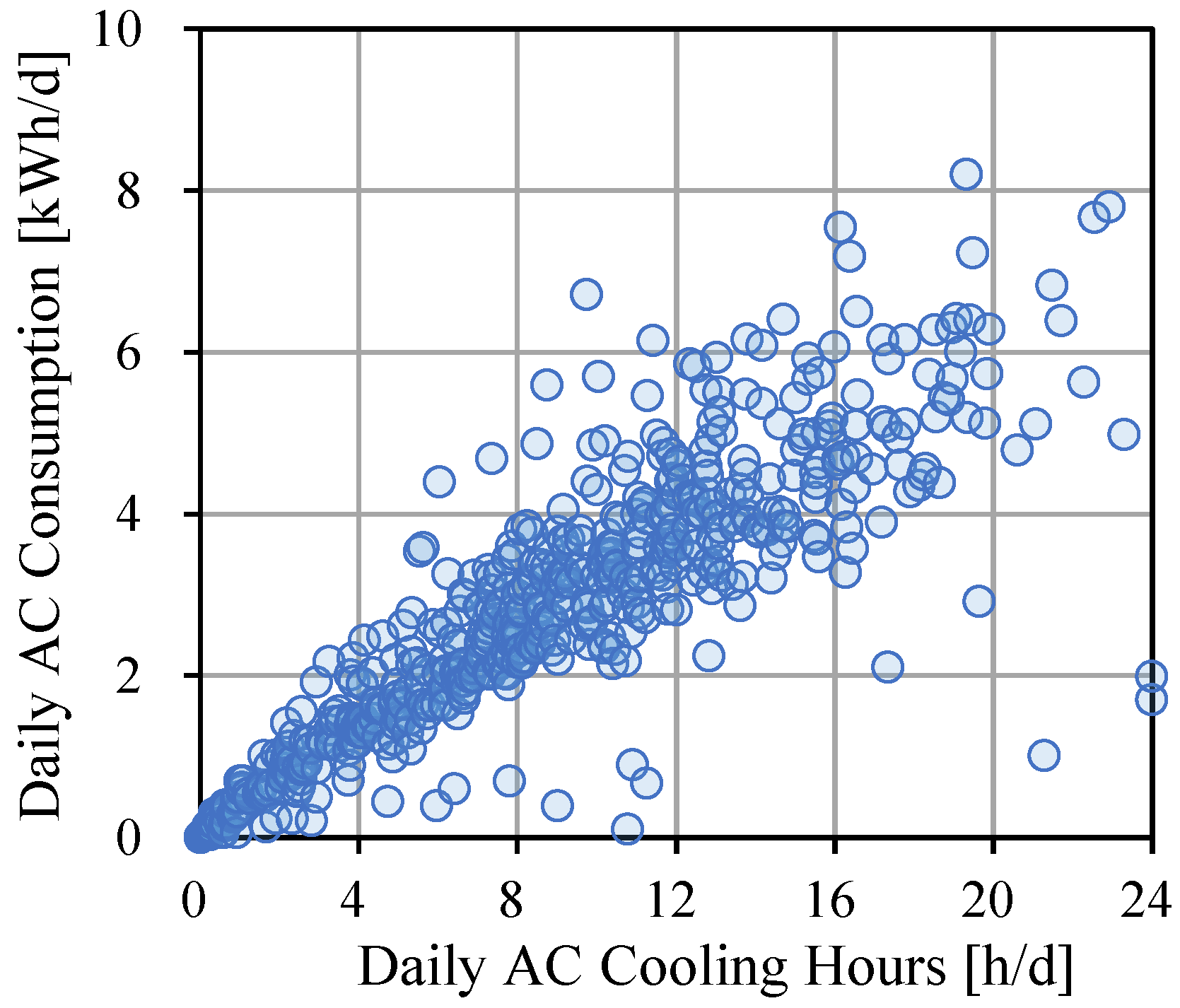
3.2. Daily AC Usage Rate

The scatter plot of daily AC cooling hours and electricity consumption in the target period is shown in Figure 4. A great diversity in cooling duration and consumption can be observed during the investigation of summer seasons, with the household’s average cooling operation ranging from 0.4 to 19 h and the electricity consumed by a room AC unit varying in the range of 10 kWh per day.

To compare cooling operation preferences among dwellings with diverse daily occupancy schedules, the AC usage range was defined in previous work as the daily cooling hours normalized by the daily hours of occupancy in the target room [30]. Figure 5 gives the density distribution of AC usage rate among the investigated 482 dwellings. Large variability in households’ reliance on cooling use could be found. The results showed that over 74% of the dwellings had an average AC usage rate of 0.3–0.7 per day. In addition, extremely active users with intensive cooling operations also accounted for around 15% of the community. Such households tended to have constant AC cooling operation during their stay in the room, with a daily AC usage rate above 0.8.

3.3. Clustering of AC Use Schedule

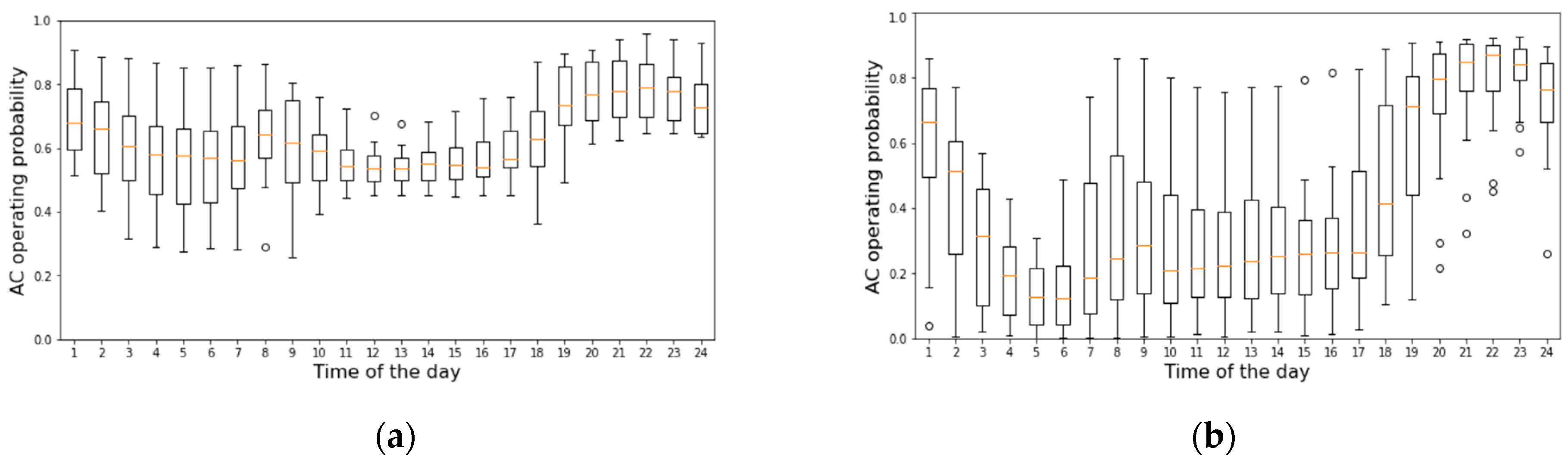
3.3.1. Hourly AC Operation Probability

The hourly AC operating probability for each dwelling was calculated using Equation (1):

$$\left({\mathit{ACPR}}_{h,i}\right)=\frac{{{\displaystyle \sum }}_{d=1}^{D}ACstat{e}_{h,d,i}}{{{\displaystyle \sum }}_{d=1}^{D}OCCstat{e}_{h,d,i}}$$

(1)

where ${\mathit{ACPR}}_{h,i}$denotes the probability of the AC operating during room-occupied hours. $ACstat{e}_{h,d,i}$indicates the AC on/off state of the hth household on the dth day of the investigation period at the ith hour, where the value is 1 if the AC was operating and 0 if the AC was not operated during the target hour.

$OCCstat{e}_{h,d,i}$indicates the room occupancy state of the hth household on the dth day of the investigation period at the ith hour. The value was 1 if the room was assumed to be occupied by at least one resident and 0 if the room was empty during the target hour.

The estimated profiles for the hourly AC operating probabilities for all 482 dwellings are shown in Figure 6. Great diversity in the daily usage schedule can be seen in the target community.

3.3.2. Clustering of Hourly AC Operating Probabilities

As mentioned above, the k-means clustering method was applied for clustering the diverse patterns of AC operating schedules of the 482 dwellings in this work. Silhouette score (SC) [31] was first selected as a metric index to determine the optimal cluster number. SC values were calculated for multiple times of k-means clustering to select the best cluster number to identify the occupant diversity. It has been confirmed that an excessively small or large number of clusters would be inappropriate for producing typical and meaningful patterns for the OBs [32]. As a result, three had the greatest SC value in this case, and it was selected as the optimal cluster number for AC use schedules.

Figure 7 shows a boxplot of the AC operating probability at each hour of the day in room-occupied periods for three clustered patterns. These three clusters can be regarded as typical preferences for AC use and are called SPA, SPB, and SPC. The main characteristic of each pattern is summarized as follows.

SPA: the group of households preferring intensive AC use regardless of the time of the day. The rate of AC operation was constantly high as long as the room was occupied by residents.

SPB: the group of households with a clear daily variation of AC uses preference with peak usage from the late afternoon to evening hours, with the AC rarely used after 1 AM or in the morning even if the occupants were at home.

SPC: the group of households preferring infrequent use of AC throughout the day. The rate of AC operation was below 0.5 within all room-occupied hours.

3.3.3. Thermal Sensitivity to AC Use Behavior for Each Household

The indoor air temperature has been widely considered a primary factor for the cooling use behavior of occupants, particularly the action of switching on the AC for thermal adaptation [33]. However, indoor air temperature is not commonly available for real-time monitoring to obtain the optimum control of building facilities or for offline analysis of building energy data such as the present study. In contrast, the outdoor air temperature is often available from a local weather station and directly or indirectly dominates the indoor thermal environment. Thus, it can also be regarded as an important variable affecting the AC use behaviors of occupants. Furthermore, previous studies on adaptive thermal comfort suggested that the outdoor air temperature has an influence on people’s thermal tolerance or perception, as characterized by the thermal comfort temperature for naturally ventilated buildings [34]. Therefore, we analyzed the relation between the outdoor air temperature and AC operation usage, considering the inter-occupant diversity.

Figure 8 and Figure 9 show the AC operating probability during the hours people were at home under different outdoor temperature conditions. This probability was defined as a 24-dimensions parameter that indicates the ratio of AC operating hours of all the room-occupied hours within the investigated period [10]. It was first calculated for each dwelling with a 2 °C resolution of outdoor air temperature, as shown in Figure 8, and statistics for the 482 dwellings are illustrated in Figure 9 as a boxplot. It should be noted that invalid probability data due to a limited sample number were already excluded.

Figure 8 shows the diverse relationship between outdoor temperature and AC use among the target community. Some households rarely used the AC when the outdoor temperature exceeded 32 °C. In contrast, several households exhibited a high probability of more than 0.9 for outdoor temperatures below 24 °C, suggesting that they continuously used the AC regardless of the outdoor thermal condition. The boxplot for the households in Figure 9 shows all the quartiles, including the median increase with an increase in the outdoor temperature, as expected. The broad ranges between the 25th and 75th percentiles under temperatures of 22–28 °C clearly illustrate the significant diversity within the community in terms of the thermal sensitivity of AC use behavior.

Our previous research has proposed thermal sensitivity as an indicator to characterize such inter-occupant diversity of thermal tolerance [10]. It was defined as the average change of AC operating probability of one dwelling with 1 °C variation of the outdoor air temperature. The thermal sensitivity level for each household (hereafter TS) was calculated based on Equation (2):

$${\mathit{TS}}_h=\frac{P_{\max ,h}-P_{0,h}}{T_{\mathrm{pmax},h}-T_{0,h}}$$

(2)

where ${\mathit{TS}}_h$denotes the thermal sensitivity of the h-th household. $P_{\max ,h}$is the maximum value of AC operating probability for the h-th household, and $P_{0,h}$represents the AC operating probability in the lowest temperature range. $T_{\mathrm{pmax},h}$ denotes the lower value for the outdoor air temperature range when the AC operating probability reaches the maximum level and $T_{0,h}$ is the lower limit for the outdoor air temperature (22 °C).

Figure 10 shows the density distribution of the household thermal sensitivity across the 482 dwellings. The horizontal axis indicates the sensitivity of the occupants to the external thermal environment change, which varied from 0 to 0.14 across the investigated dwellings. In other words, a household increased their probability of using AC by up to 0.14 with a 1 °C increase in the outdoor temperature.

3.3.4. Household Clustering Based on Thermal Preference

Based on the daily AC use rate shown in Figure 4 and household thermal sensitivity shown in Figure 10, we applied k-means clustering to classify representative groups of households as an influential factor underlying the diverse AC use schedules among households. In this case, the optimal clustering number was determined to be four, which was calculated with the greatest SC value for thermal preference. The clustering results are illustrated in Figure 11. Four typical thermal preference patterns were found with a different share of the dwellings in the community.

TPA: households that were sensitive to an outdoor temperature variation and had intensive cooling use.

TPB: households that were sensitive to an outdoor temperature variation but had inactive cooling use.

TPC: households with intensive cooling use regardless of the ambient thermal environment.

TPD: households that were insensitive to the outdoor temperature variation and had rare cooling use.

Thermally sensitive users (TPA and TPB) were found to be the majority in the investigated community. Both households assigned in the pattern of TPA (sensitive and active) and TPB (sensitive but non-active) showed a tendency of adaptive behavior, meaning an increase in AC use with a temperature rise. In contrast, households with intensive AC cooling usage in various thermal conditions and showed no behavioral change also existed (TPC) and accounted for 19% of the community. Such household-level labeling based on thermal preference was used as OB-related input information for the AC operation prediction model in the following section.

4. AC on/off State Modeling

4.1. XGBoost Model Establishment

Based on the clustering analysis results for the occupants’ operating schedule preferences and thermal preferences shown in previous sections, such behavioral variables, namely the schedule preference type and thermal sensitivity type, were used as the input features for the XGBoost model to reproduce the inter-occupant diversity. In addition, the real-time outdoor temperature and historical weighted temperature, T_weighted, were also included as inputs for the prediction.

T_weighted was proposed by Lyu et al. [30] to consider the influence of the outdoor temperature on previous days on AC use, as expressed by Equation (3):

$$T_{\mathrm{weighted}}={\displaystyle \sum }_{i=0}^n\left(w_i\cdot T_i\right)/{\displaystyle \sum }_{i=0}^n{w}_i$$

(3)

where i indicates the number of days elapsed from the target date of interest, n is the maximum number of elapsed days to be involved as the influential period of past thermal exposure, and w_i denotes the weight factor of the ith-day, which exponentially decreases with each day elapsed, meaning the decreasing significance of the past days as time progresses. The inputs and outputs of the model are listed in

Table 4. Inputs and outputs of the XGBoost model.

	Variables	Remarks
Input	Hour	Categorical (0, 1, 2 …23)
	Outdoor air temperature	Continuous
	Thermal sensitivity type	Categorical (TPA, TPB, TPC, TPD)
	Schedule preference type	Categorical (SPA, SPB, SPC)
	Weighted mean temperature (10 days)	Continuous
Output	AC on/off state	1: ON; 0: OFF

. A binary variable indicating the hourly AC on/off state throughout the target season, with a value of 1 indicating AC operation at the target hour and 0 indicating the opposite, was generated as the output of this model.

4.2. Hyperparameter Optimization

The dataset was first divided into two groups for training and testing data. The training group contained 70% of the total samples and was used to learn and optimize the parameters of the model. The other 30% was used for testing the prediction performance of the model. K-fold cross-validation [35] was then applied, which splits training data into a K number of folds to evaluate the model’s ability when given new data. In this work, a five-fold cross-validation process was conducted.

The next step was to obtain the optimal hyperparameters, which denote certain values or weights of the model used to control the learning process of its gradient-boosting algorithm. Hyperparameters in the tree-based algorithm determine the detailed settings of the structure, such as the maximum depth of the tree, the number of trees to grow, and feature weights to prevent overfitting. Grid search [36], as a common tool for hyperparameter tuning, was applied in this work to obtain the optimal model settings. It works as an exhaustive search over every combination of specified parameter values. After specifying several possible values for the main hyperparameters, the optimal parameters for the model were determined by the optimizer, as listed in

Table 5. Setting of the parameters in the XGBoost model.

Parameters	Range	Description	Settings
training group		Data for parameter learning	70%
testing group		Data for performance testing	30%
n_esitimators	[50, 150, 300, 500]	Number of gradient-boosted trees	150
leaning rate	[0.01, 0.05, 0.1, 0.3]	Feature weights to prevent overfitting	0.1
max_depth	[4, 6, 8, 10]	Maximum tree depth for base learners	6
min_child_weight	[5, 6, 7, 8]	Minimum sum of instance weight	5
gamma	[0.2, 0.4, 0.6, 0.8]	Minimum loss reduction required for a further partition	0.6

. The performance of the proposed XGBoost model was evaluated, and the results are discussed in the following section.

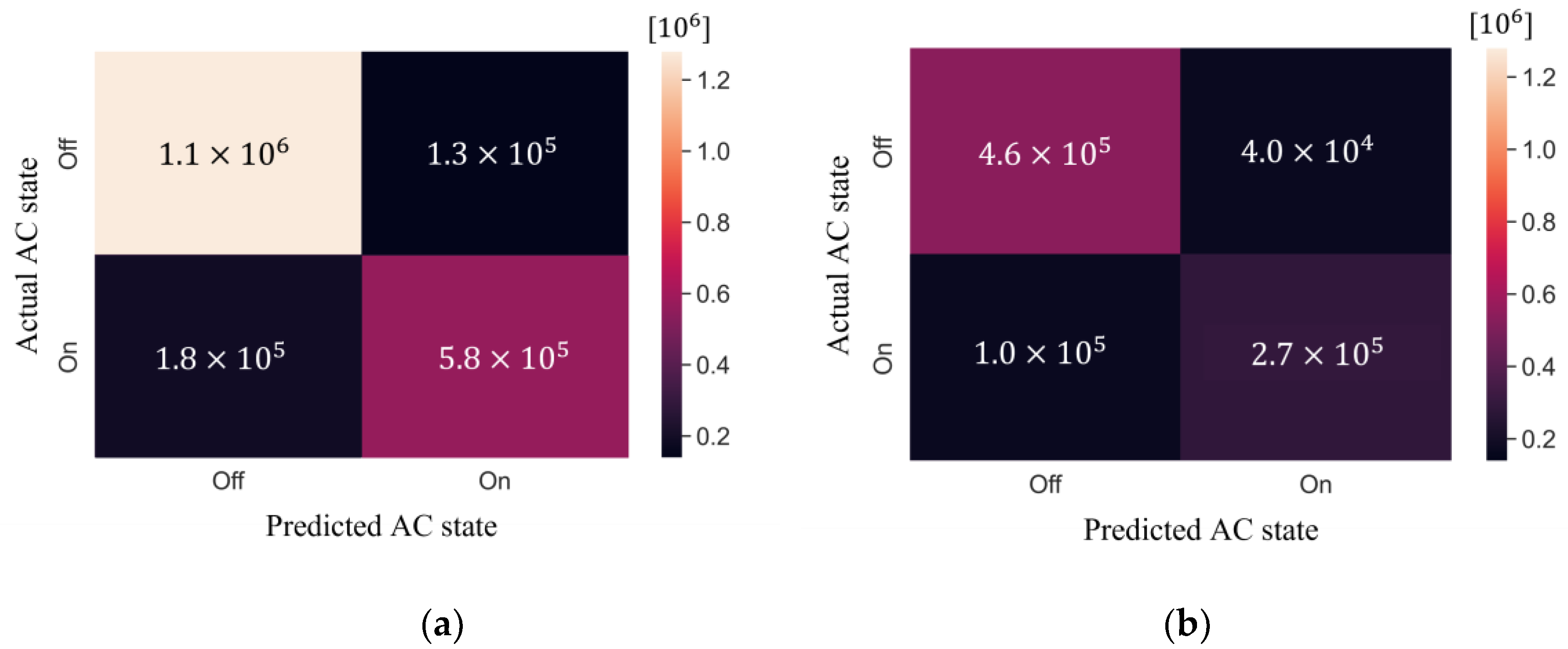
4.3. Modeling Performance Evaluation

Considering the imbalanced distribution of AC on and off states, a confusion matrix [37] was applied for model assessment. The binary results for the predicted AC operation states for each hour were divided into positive and negative values, with four key parameters: true positive (TP), true negative (TN), false positive (FP), and false negative (FN). Multiple widely used indicators for model evaluation [29,38] were defined based on the following equations. The accuracy gives the percentage of correct classifications of the AC on/off state.

$$Accuracy=\frac{TP+TN}{TP+TN+FP+FN}$$

(4)

$$Recall=\frac{TP}{P}=\frac{TP}{TP+FN}$$

(5)

$$Precision=\frac{TP}{TP+FP}$$

(6)

where TP denotes results that are actually positive and were predicted to be positive, and TN denotes results that are actually negative and were predicted to be negative. FN denotes results that are actually positive but were predicted to be negative. FP denotes results that are actually negative but were predicted to be positive. P denotes results that are actually positive (TP and FN), and N denotes results that are actually negative (TN and FP). The F1 score was also calculated as an indicator weighting the recall and precision, with a value closer to one indicating that the prediction model was more accurate.

$$F1 score=\frac{2\bullet precision\bullet recall}{precision+recall}$$

(7)

5. Results and Discussion

5.1. Results

Figure 12 shows the confusion matrix of the established XGBoost model for the prediction of AC on/off states in both training and testing groups. The confusion matrix is a table presenting the actual and predicted states of AC operation in each time step, with the diagonal elements indicating the number of correctly predicted operation states.

Table 6. Prediction performance of the model in both the training and testing group.

	Accuracy	Recall	Precision	F1 Score
Training group	0.83	0.76	0.82	0.79
Testing group	0.82	0.73	0.85	0.80

gives the Prediction performance of the model in both the training and testing group. Recall here denotes the fraction of AC on states in all time steps that have been correctly predicted by the model, and precision denotes the percentage of the correctly predicted AC on the state in all the prediction results. It was found that the proposed model shows satisfying performance with high precision, recall, and accuracy in identifying the AC operation states. The F1 score of the XGBoost model was 0.79 and 0.80 for training and testing data, respectively.

Figure 13 shows a receiver operating characteristics (ROC) curve, which indicates the performance of the AC state prediction. The vertical axis shows the TP rate, and the horizontal axis shows the FP rate. The Area Under the ROC Curve (AUC) value represents the entire two-dimensional area underneath the entire ROC curve, indicating in broad terms the model’s ability to predict classes correctly. The AUC score ranges from 0 to 1, where 1 is a perfect score and 0.5 means the model is as good as random. The results show an AUC value of 0.845, indicating a high chance that the classifier will be able to distinguish the positive class values from the negative class values.

Figure 14 gives the feature importance scores for the prediction model. The scores of the input features were assigned based on their importance in predicting the output. A higher score indicated that the feature was more responsible and influential in predicting the AC on/off state. The results show that the schedule preference and thermal preference patterns both had large effects on the prediction of the AC state, with feature importance scores of occupants’ schedule preference and thermal preference in AC state prediction found to be 0.384 and 0.263, respectively. In other words, these two factors could be recognized as effectively representing the inter-occupant diversity in AC use behavior. Moreover, the real-time ambient temperature and historical mean temperature, T_weighted, showed similar feature importance values, proving that the impact of the outdoor temperature on AC use conceivably changes over time within a certain time period.

5.2. Applications and Limitations

In this study, a prediction model of residential AC usage considering diverse behavioral patterns was established with satisfactory performance. The main contribution of the proposed work is that informative and realistic references could be provided for researchers focusing on the modeling and prediction of OB in AC usage. For example, the identification process of a household’s thermal and schedule preference for cooling usage could be considered for generalization to similar modeling of AC usage at the community or regional level for other studies. Further, the representative patterns for occupancy and AC operation schedules derived in this study could be helpful in similar large-scale case studies. It would be a good reference for the stochastic and complex nature of occupants’ behavioral patterns rather than a basic and fixed standard.

As one of the limitations of this study, the prediction model included only the real-time outdoor air temperature and weighted mean outdoor temperature in a historical period as the input information of external conditions. The indoor temperature, another influencing factor of AC operation, could not be involved due to the limitation of data availability. As a result, the prediction of AC on/off state in this work could not be associated with the variation of the indoor thermal environment. In addition, the energy dataset used in this study was measured and collected in 2013 and 2014 in Osaka, Japan. Considering the mechanism of occupants’ climatic-responsive behaviors, the unavailability of more recent data has little effect on the current findings. Although the methodology of this work could be derived towards wider generalization, the differences in occupants’ preferences and climate conditions, as well as possible AC module advancements, should be considered for our future studies in other regions.

6. Conclusions

This work proposed a prediction method for the stochastic AC on/off state in a residential building considering the inter-occupant diversity of AC use behavior based on the appliance-level electricity demand data for 482 dwellings in a real community during two consecutive cooling seasons. Statistical analysis was first conducted to identify the inter-occupant diversity of OBs in the measured dwellings. In particular, individual preferences regarding occupancy schedules, daily cooling schedules, and thermal sensitivity were found to show great variability across the community. Clustering analysis was then applied to classify the dwellings into different schedules and thermal preference patterns. The XGBoost model was applied to predict the hourly AC on/off state and showed satisfactory performance. The main conclusions are summarized as follows.

• Great diversity in the inter-occupant behavioral preferences related to AC usage was found in the target community.
• Three and four types of households were identified for the occupants’ behaviors related to their cooling schedule and thermal sensitivity patterns, respectively.
• The proposed model considering diverse OBs, showed satisfactory prediction performance, with an AUC score of 0.845, indicating a high chance of accurate distinguishment of AC operation states.
• Instead of the outdoor temperature, the behaviors of the occupants were found to have a crucial impact on a household’s AC operation. Feature importance scores of occupants’ schedule preference and thermal preference in AC state prediction were found to be 0.384 and 0.263, respectively.

References

1. UNEP. 2022 Global Status Report for Buildings and Construction. Available online: https://www.unep.org/resources/publication/2022-global-status-report-buildings-and-construction (accessed on 1 December 2022).
2. Dai, B.; Liu, C.; Liu, S.; Wang, D.; Wang, Q.; Zou, T.; Zhou, X. Life cycle techno-enviro-economic assessment of dual-temperature evaporation transcritical CO2 high-temperature heat pump systems for industrial waste heat recovery. Appl. Therm. Eng. 2023, 219, 119570. [Google Scholar] [CrossRef]
3. Yousefi, F.; Gholipour, Y.; Yan, W. A study of the impact of occupant behaviors on energy performance of building envelopes using occupants’ data. Energy Build 2017, 148, 182–198. [Google Scholar] [CrossRef]
4. Blight, T.S.; Coley, D.A. Sensitivity analysis of the effect of occupant behaviour on the energy consumption of passive house dwellings. Energy Build 2013, 66, 183–192. [Google Scholar] [CrossRef]
5. Ranjbar, N.; Zaki, S.A.; Yusoff, N.M.; Yakub, F.; Hagishima, A. Short-term measurements of household electricity demand during hot weather in Kuala Lumpur. Int. J. Electr. Comput. Eng. 2017, 7, 1436. [Google Scholar] [CrossRef]
6. Sena, B.; Zaki, S.; Rijal, H.; Ardila-Rey, J.; Yusoff, N.; Yakub, F.; Ridwan, M.; Muhammad-Sukki, F. Determinant factors of electricity consumption for a Malaysian household based on a field survey. Sustainability 2021, 13, 818. [Google Scholar] [CrossRef]
7. Murtyas, S.; Ridwan, M.; Budiarto, R. Occupancy Rate and Water Utility Effects on Energy Consumption of Commercial Building: Case Study Grand Inna Malioboro Hotel in Indonesia; Interdisciplinary Graduate School of Engineering Sciences, Kyushu University: Fukuoka, Japan, 2019. [Google Scholar]
8. Yun, G.Y.; Steemers, K. Behavioural, physical and socio-economic factors in household cooling energy consumption. Appl. Energy 2011, 88, 2191–2200. [Google Scholar] [CrossRef]
9. Hong, T.; Yan, D.; D’Oca, S.; Chen, C.-F. Ten questions concerning occupant behavior in buildings: The big picture. Build Environ. 2017, 114, 518–530. [Google Scholar] [CrossRef]
10. Lyu, J.; Hagishima, A. Occupant’s Thermal Preference Diversity in Residential Air-Conditioning Use: A Study in Osaka, Japan; Interdisciplinary Graduate School of Engineering Sciences, Kyushu University: Fukuoka, Japan, 2022. [Google Scholar]
11. Clevenger, C.M.; Haymaker, J. The impact of the building occupant on energy modeling simulations. In Proceedings of the Joint International Conference on Computing and Decision Making in Civil and Building Engineering, Montreal, Canada, 14–16 June 2006; pp. 1–10. [Google Scholar]
12. Ren, X.; Yan, D.; Wang, C. Air-conditioning usage conditional probability model for residential buildings. Build Environ. 2014, 81, 172–182. [Google Scholar] [CrossRef]
13. Tanimoto, J.; Hagishima, A. Total utility demand prediction system for dwellings based on stochastic processes of actual inhabitants. J. Build Perform. Simul. 2010, 3, 155–167. [Google Scholar] [CrossRef]
14. Yao, J. Modelling and simulating occupant behaviour on air conditioning in residential buildings. Energy Build 2018, 175, 1–10. [Google Scholar] [CrossRef]
15. Diao, L.; Sun, Y.; Chen, Z.; Chen, J. Modeling energy consumption in residential buildings: A bottom-up analysis based on occupant behavior pattern clustering and stochastic simulation. Energy Build 2017, 147, 47–66. [Google Scholar] [CrossRef]
16. Xia, D.; Lou, S.; Huang, Y.; Zhao, Y.; Li, D.H.; Zhou, X. A study on occupant behaviour related to air-conditioning usage in residential buildings. Energy Build 2019, 203, 109446. [Google Scholar] [CrossRef]
17. Mun, S.H.; Kwak, Y.; Huh, J.H. A case-centered behavior analysis and operation prediction of AC use in residential buildings. Energy Build 2019, 188, 137–148. [Google Scholar] [CrossRef]
18. Chen, T.; Guestrin, C. Xgboost: A scalable tree boosting system. In Proceedings of the 22nd ACM Sigkdd International Conference on Knowledge Discovery and Data Mining, San Francisco, CA, USA, 13–17 August 2016; pp. 785–794. [Google Scholar]
19. Wang, Z.; Hong, T.; Piette, M.A. Building thermal load prediction through shallow machine learning and deep learning. Appl. Energy 2020, 263, 114683. [Google Scholar] [CrossRef]
20. Yan, L.; Liu, M. A simplified prediction model for energy use of air conditioner in residential buildings based on monitoring data from the cloud platform. Sustain. Cities Soc. 2020, 60, 102194. [Google Scholar] [CrossRef]
21. Yan, L.; Liu, M. Predicting household air conditioners’ on/off state considering occupants’ preference diversity: A study in Chongqing, China. Energy Build 2021, 253, 111516. [Google Scholar] [CrossRef]
22. Zaki, S.A.; Hagishima, A.; Fukami, R.; Fadhilah, N. Development of a model for generating air-conditioner operation schedules in Malaysia. Build Environ. 2017, 122, 354–362. [Google Scholar] [CrossRef]
23. Fukami, R.; Hagishima, A.; Tanimoto, J.; Ikegaya, N. Stochastic nature of occupants’ behavior toward air-conditioning operation in residential buildings. J. Archit. Rev. 2022, 5, 649–660. [Google Scholar] [CrossRef]
24. MacQueen, J. Classification and analysis of multivariate observations. In Proceedings of the 5th Berkeley Symp Math Statist Probab, Berkeley, CA, USA, 21 June–18 July 1965 and 27 December 1965–7 January 1966; pp. 281–297. [Google Scholar]
25. Jain, A.K. Data clustering: 50 years beyond K-means. Pattern Recognit. Lett. 2010, 31, 651–666. [Google Scholar] [CrossRef]
26. Buitinck, L.; Louppe, G.; Blondel, M.; Pedregosa, F.; Mueller, A.; Grisel, O.; Niculae, V.; Prettenhofer, P.; Gramfort, A.; Grobler, J.; et al. API design for machine learning software: Experiences from the scikit-learn project. arXiv 2013, arXiv:1309.0238. [Google Scholar]
27. Wakjira, T.G.; Ebead, U.; Alam, M.S. Machine learning-based shear capacity prediction and reliability analysis of shear-critical RC beams strengthened with inorganic composites. Case Stud. Constr. Mater. 2022, 16, e01008. [Google Scholar] [CrossRef]
28. Wakjira, T.G.; Rahmzadeh, A.; Alam, M.S.; Tremblay, R. Explainable machine learning based efficient prediction tool for lateral cyclic response of post-tensioned base rocking steel bridge piers. Structures 2022, 44, 947–964. [Google Scholar] [CrossRef]
29. Zhou, X.; Ren, J.; An, J.; Yan, D.; Shi, X.; Jin, X. Predicting open-plan office window operating behavior using the random forest algorithm. J. Build Eng. 2021, 42, 102514. [Google Scholar] [CrossRef]
30. Lyu, J.; Ono, T.; Sato, A.; Hagishima, A.; Tanimoto, J. Seasonal variation of residential cooling use behaviour derived from energy demand data and stochastic building energy simulation. J. Build Eng. 2022, 49, 104067. [Google Scholar] [CrossRef]
31. Rousseeuw, P.J. Silhouettes: A graphical aid to the interpretation and validation of cluster analysis. J. Comput. Appl. Math. 1987, 20, 53–65. [Google Scholar] [CrossRef]
32. Ma, Z.; Yan, R.; Nord, N. A variation focused cluster analysis strategy to identify typical daily heating load profiles of higher education buildings. Energy 2017, 134, 90–102. [Google Scholar] [CrossRef]
33. Song, Y.; Sun, Y.; Luo, S.; Tian, Z.; Hou, J.; Kim, J.; Parkinson, T.; de Dear, R. Residential adaptive comfort in a humid continental climate—Tianjin China. Energy Build 2018, 170, 115–121. [Google Scholar] [CrossRef]
34. ASHRAE. Standard 55-Thermal Environmental Conditions for Human Occupancy; ASHRAE: Peachtree Corners, GA, USA, 2017. [Google Scholar]
35. Ng, A.Y. Preventing “overfitting” of cross-validation data. In Proceedings of the Fourteenth International Conference on Machine Learning, ICML, Nashville, TN, USA, 8–12 July 1997; Volume 97, pp. 245–253. [Google Scholar]
36. LaValle, S.M.; Branicky, M.S.; Lindemann, S.R. On the relationship between classical grid search and probabilistic roadmaps. Int. J. Robot. Res. 2004, 23, 673–692. [Google Scholar] [CrossRef]
37. Fawcett, T. An introduction to ROC analysis. Pattern. Recognit. Lett. 2006, 27, 861–874. [Google Scholar] [CrossRef]
38. Markovic, R.; Grintal, E.; Wölki, D.; Frisch, J.; van Treeck, C. Window opening model using deep learning methods. Build Environ. 2018, 145, 319–329. [Google Scholar] [CrossRef] [Green Version]
Figure 1. Variation in the daily average outdoor air temperature from June to September in Osaka.
Buildings 13 00521 g001
Figure 2. Scheme of hourly occupancy schedule detection.
Buildings 13 00521 g002
Figure 3. Example of detected daily occupancy and cooling usage patterns for one household.
Buildings 13 00521 g003
Figure 4. Scatter plot of average cooling hours and AC electricity consumption for each household per day.
Buildings 13 00521 g004
Figure 5. Density distribution of daily average AC usage rate across the 482 investigated dwellings.
Buildings 13 00521 g005
Figure 6. Hourly AC operating probabilities for all 482 dwellings.
Buildings 13 00521 g006
Figure 7. Box plot of AC operating probabilities for three clusters. (a) Schedule Preference A (SPA). (b) Schedule Preference B (SPB). (c) Schedule Preference C (SPC).
Buildings 13 00521 g007aBuildings 13 00521 g007b
Figure 8. AC operating probability in different outdoor air temperature ranges for all 486 dwellings [10].
Buildings 13 00521 g008
Figure 9. Boxplot of AC operating probability in different outdoor air temperature ranges [10].
Buildings 13 00521 g009
Figure 10. Density distribution of the household thermal sensitivity across the 482 investigated dwellings [10].
Buildings 13 00521 g010
Figure 11. Clustering results of thermal preference patterns across 482 dwellings. (a) Four typical clusters of thermal preference pattern. (b) Share of each cluster.
Buildings 13 00521 g011
Figure 12. Confusion matrix of XGBoost model in (a) training group and (b) testing group.
Buildings 13 00521 g012
Figure 13. ROC curve of the prediction model.
Buildings 13 00521 g013
Figure 14. Normalized results for feature importance scores in AC on/off state prediction.
Buildings 13 00521 g014