
Analyzing Electricity Consumption Factors of Buildings in Seoul, Korea Using Multiscale Geographically Weighted Regression


Abstract
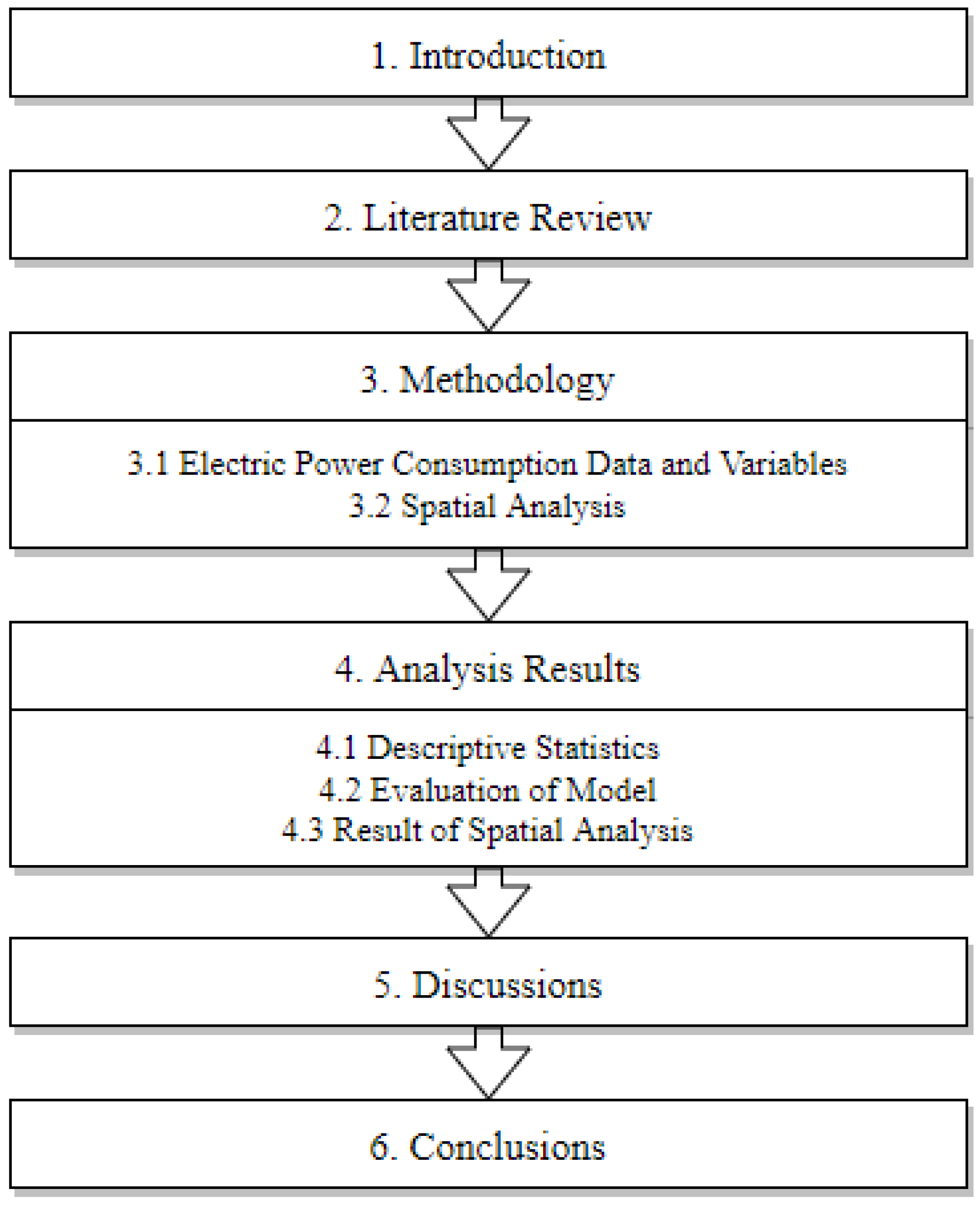
:1. Introduction
2. Literature Review
3. Methodology
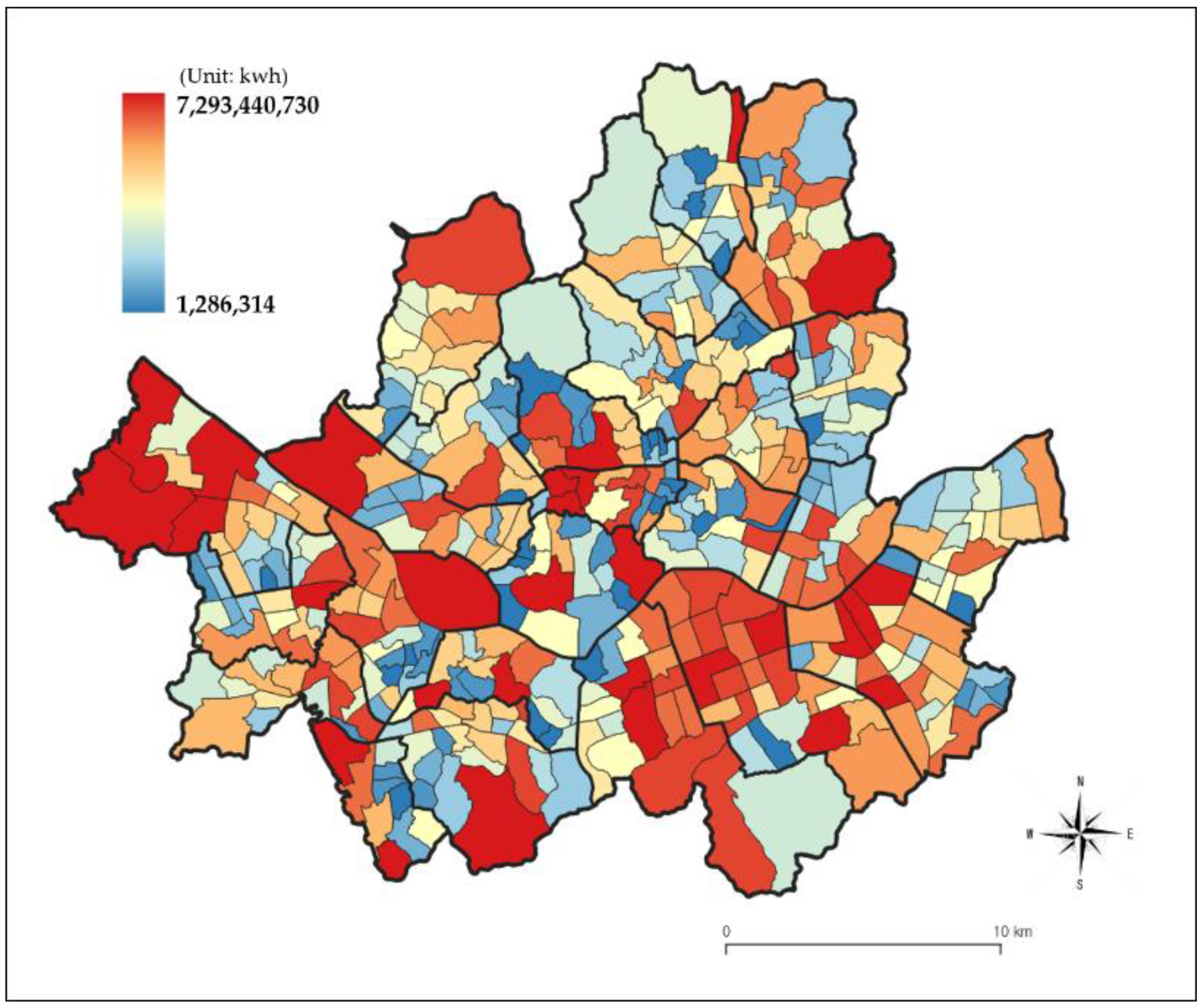
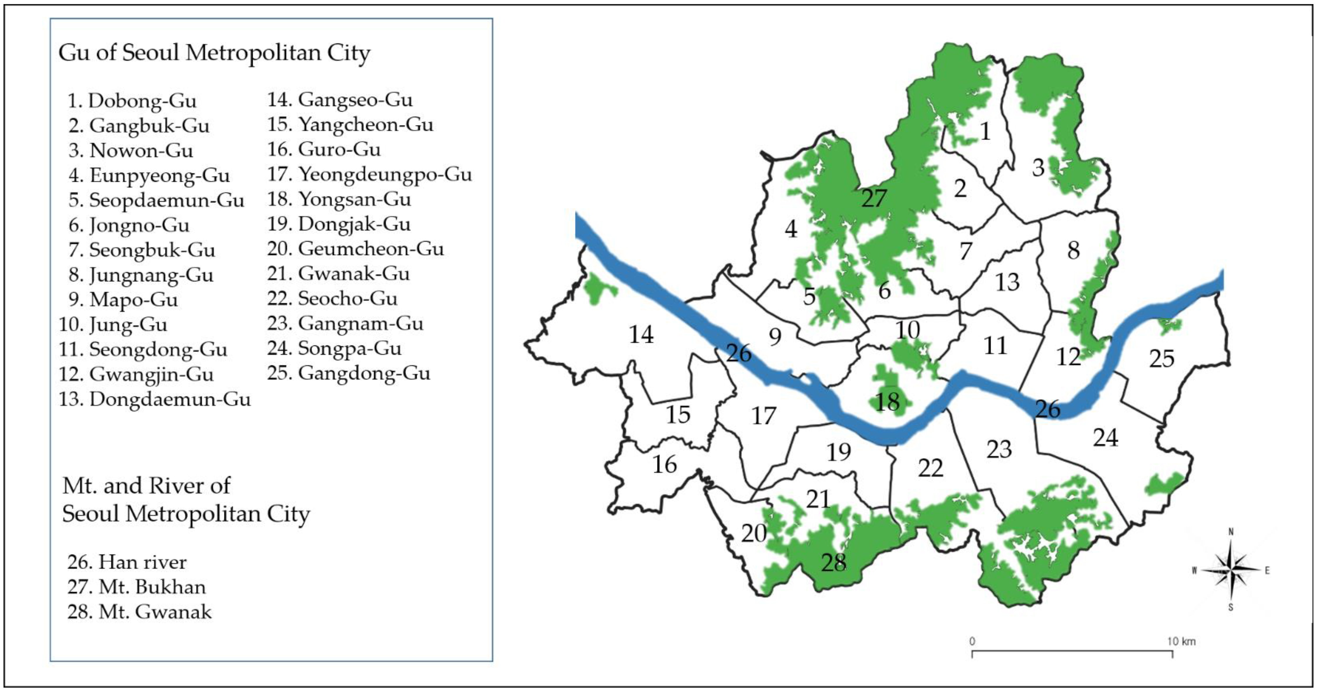
3.1. Electric Power Consumption Data and Variables
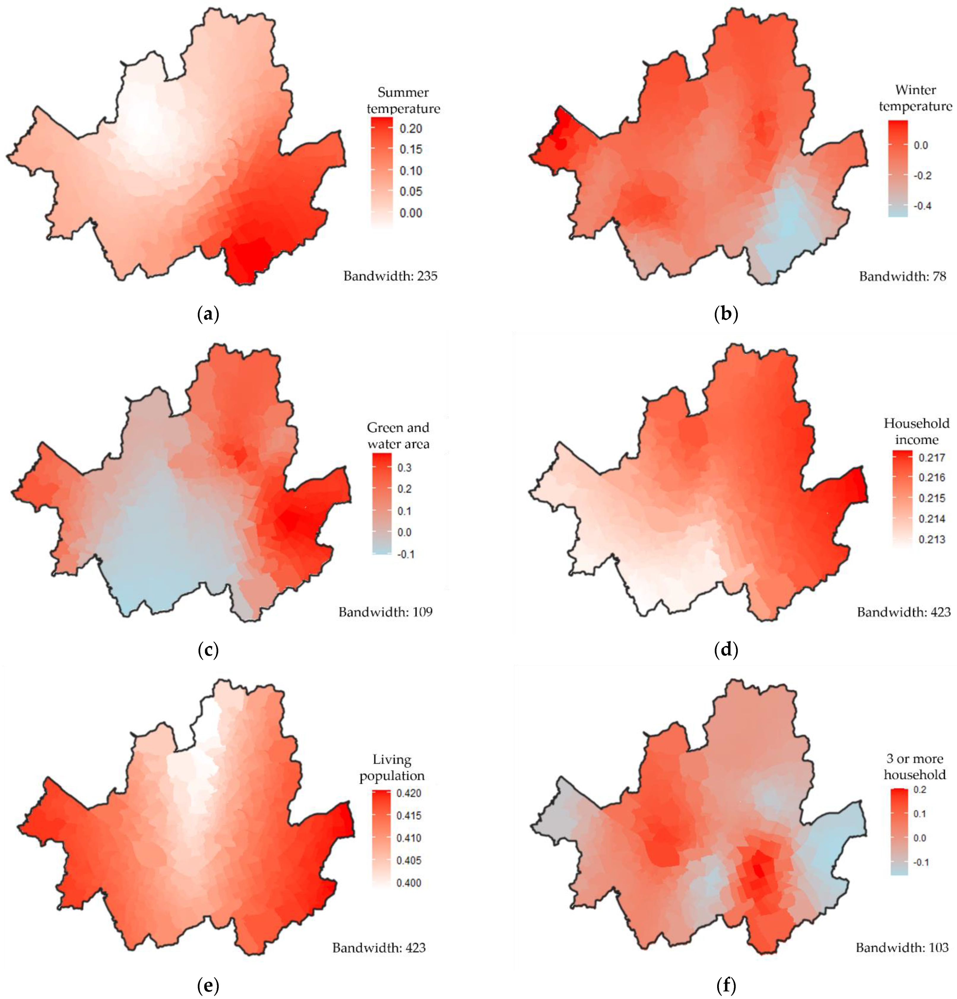
3.2. Spatial Analysis
3.2.1. GWR
3.2.2. Multiscale GWR
4. Analysis Results
4.1. Descriptive Statistics
4.2. Evaluation of Model
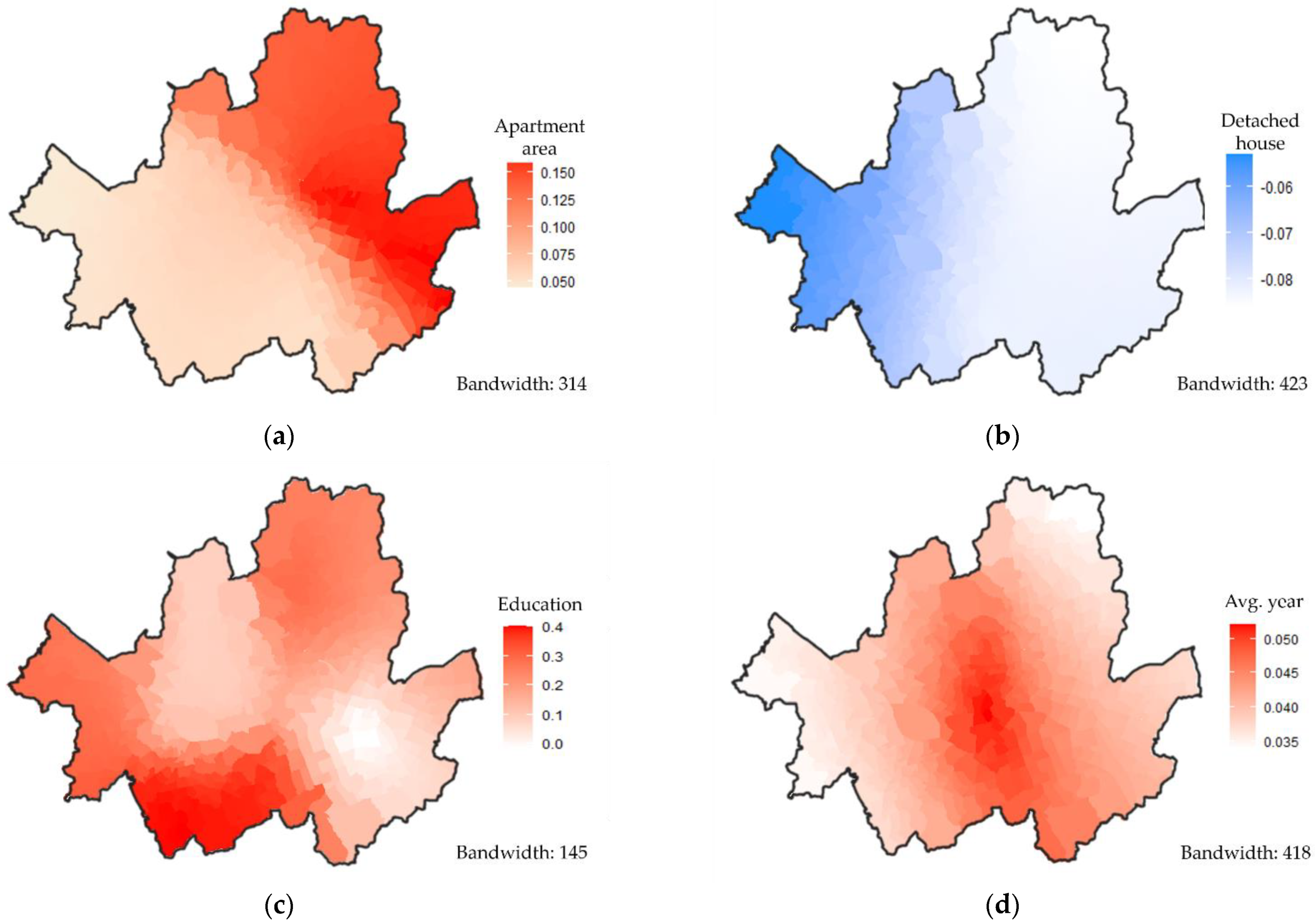
4.3. Result of Spatial Analysis
5. Discussions
6. Conclusions
Author Contributions
Funding
Institutional Review Board Statement
Informed Consent Statement
Data Availability Statement
Conflicts of Interest
References
- IPCC. Climate Change 2021: The Physical Science Basis. IPCC Sixth Assess. Rep. 2022, 12, 142. [Google Scholar]
- Mostafavi, F.; Tahsildoost, M.; Zomorodian, Z. Energy efficiency and carbon emission in high-rise buildings: A review (2005–2020). Build. Environ. 2021, 206, 108329. [Google Scholar] [CrossRef]
- Steemers, K. Energy and the city: Density, buildings and transport. Energy Build. 2003, 35, 3–14. [Google Scholar] [CrossRef]
- Chen, H.; Zhu, Q.; Peng, C.; Wu, N.; Wang, Y.; Fang, X.; Gao, Y.; Zhu, D.; Yang, G.; Tian, J.; et al. The impacts of climate change and human activities on biogeochemical cycles on the Qinghai-Tibetan Plateau. Glob. Change Biol. 2013, 19, 2940–2955. [Google Scholar] [CrossRef] [PubMed]
- Amanatidis, G. European Policies on Climate and Energy towards 2020, 2030 and 2050. Policy Commons 2019, 631, 47. [Google Scholar]
- Global Alliance for Buildings and Construction. International Energy Agency and the United Nations Environment Programme 2019 global status report for buildings and construction: Towards a zero-emission, efficient and resilient buildings and construction sector. United Nations Environ. Programme 2019, 10, 2265. [Google Scholar]
- Nord, N. Building energy efficiency in cold climates. Encycl. Sustain. Technol. 2017, 149–157. [Google Scholar]
- Chen, Y.; Hong, T. Impacts of building geometry modeling methods on the simulation results of urban building energy models. Appl. Energy 2018, 215, 717–735. [Google Scholar] [CrossRef] [Green Version]
- Li, C.; Song, Y.; Kaza, N. Urban form and household electricity consumption: A multilevel study. Energy Build. 2018, 158, 181–193. [Google Scholar] [CrossRef]
- Ahn, Y.; Sohn, D.W. The effect of neighbourhood-level urban form on residential building energy use: A GIS-based model using building energy benchmarking data in Seattle. Energy Build. 2019, 196, 124–133. [Google Scholar] [CrossRef]
- Sena, B.; Zaki, S.A.; Rijal, H.B.; Alfredo Ardila-Rey, J.; Yusoff, N.M.; Yakub, F.; Ridwan, M.K.; Muhammad-Sukki, F. Determinant factors of electricity consumption for a Malaysian household based on a field survey. Sustainability 2021, 13, 818. [Google Scholar] [CrossRef]
- Swan, L.G.; Ugursal, V.I. Modeling of end-use energy consumption in the residential sector: A review of modeling techniques. Renew. Sustain. Energy Rev. 2009, 13, 1819–1835. [Google Scholar] [CrossRef]
- Choi, I.Y.; Cho, S.H.; Kim, J.T. Energy consumption characteristics of high-rise apartment buildings according to building shape and mixed-use development. Energy Build. 2012, 46, 123–131. [Google Scholar] [CrossRef]
- Woo, Y.E.; Cho, G.H. Impact of the surrounding built environment on energy consumption in mixed-use building. Sustainability 2018, 10, 832. [Google Scholar] [CrossRef] [Green Version]
- Qiao, R.; Liu, T. Impact of building greening on building energy consumption: A quantitative computational approach. J. Clean. Prod. 2020, 246, 119020. [Google Scholar] [CrossRef]
- Zhao, J.; Zhu, N.; Wu, Y. The analysis of energy consumption of a commercial building in Tianjin, China. Energy Policy 2009, 37, 2092–2097. [Google Scholar] [CrossRef]
- Campagna, L.M.; Fiorito, F. On the Impact of Climate Change on Building Energy Consumptions: A Meta-Analysis. Energies 2022, 15, 354. [Google Scholar] [CrossRef]
- Zhang, J.; Zhang, K.; Zhao, F. Research on the regional spatial effects of green development and environmental governance in China based on a spatial autocorrelation model. Struct. Change Econ. Dyn. 2020, 55, 1–11. [Google Scholar] [CrossRef]
- Fonseca, J.A.; Schlueter, A. Integrated model for characterization of spatiotemporal building energy consumption patterns in neighborhoods and city districts. Appl. Energy 2015, 142, 247–265. [Google Scholar] [CrossRef]
- Wang, H.; Pan, X.; Zhang, S. Spatial autocorrelation, influencing factors and temporal distribution of the construction and demolition waste disposal industry. Waste Manag. 2021, 127, 158–167. [Google Scholar] [CrossRef]
- Tian, W.; Song, J.; Li, Z. Spatial regression analysis of domestic energy in urban areas. Energy 2014, 76, 629–640. [Google Scholar] [CrossRef]
- Mostafavi, N.; Heris, M.P.; Gándara, F.; Hoque, S. The Relationship between Urban Density and Building Energy Consumption. Buildings 2021, 11, 455. [Google Scholar] [CrossRef]
- Miller, H.J. Tobler’s first law and spatial analysis. Ann. Assoc. Am. Geogr. 2004, 94, 284–289. [Google Scholar] [CrossRef]
- Noh, S. Analysis of Energy Consumption and CO2 Emissions Structure in Household Sector. Korea Spat. Plan. Rev. 2014, 81, 157–183. [Google Scholar]
- Jung, J.; Yi, C.; Lee, S. An Integrative Analysis of the Factors Affecting the Household Energy Consumption in Seoul. J. Korea Plan. Assoc. 2015, 50, 75–94. [Google Scholar] [CrossRef]
- Kim, K.J.; Lee, C.H. A Study on the Difference of Cooling Energy Consumption by Building Use. Seoul Stud. 2019, 20, 91–103. [Google Scholar]
- Lee, G.; Jeong, Y.; Moon, Y.D. The Relation of between the Architectural and Urban Form, Microclimate Factors and Buildings Energy Consumption. Asia-Pac. J. Multimed. Serv. Converg. Art Humanit. Sociol. 2019, 9, 923–934. [Google Scholar]
- Lee, S.; Kim, K.; Lee, S. Empirical Analysis of Mutual Influential Relationship between Urban Temperature and Building Energy Consumption Using Simultaneous Equation—Focused on Seoul, Korea. Seoul Stud. 2019, 20, 33–44. [Google Scholar] [CrossRef]
- Kim, D.H.; Kang, K.Y.; Sohn, S.Y. Spatial Pattern Analysis of CO2 Emission in Seoul Metropolitan City based on a Geographically Weighted regression. J. Korean Inst. Ind. Eng. 2016, 42, 96–111. [Google Scholar]
- Mohammadi, N.; Taylor, J.E. Urban infrastructure-mobility energy flux. Energy 2017, 140, 716–728. [Google Scholar] [CrossRef]
- Santamouris, M.; Cartalis, C.; Synnefa, A.; Kolokotsa, D. On the impact of urban heat island and global warming on the power demand and electricity consumption of buildings—A review. Energy Build. 2015, 98, 119–124. [Google Scholar] [CrossRef]
- Lee, J.; Kim, J.; Song, D.; Kim, J.; Jang, C. Impact of external insulation and internal thermal density upon energy consumption of buildings in a temperate climate with four distinct seasons. Renew. Sustain. Energy Rev. 2017, 75, 1081–1088. [Google Scholar] [CrossRef]
- Aditya, L.; Mahlia, T.M.I.; Rismanchi, B.; Ng, H.M.; Hasan, M.H.; Metselaar, H.S.C.; Muraza, O.; Aditiya, H.B. A review on insulation materials for energy conservation in buildings. Renew. Sustain. Energy Rev. 2017, 73, 1352–1365. [Google Scholar] [CrossRef]
- Sadrzadehrafiei, S.; Mat, K.S.S.; Lim, C. Energy consumption and energy saving in Malaysian office buildings. Models Methods Appl. Sci. 2011, 75, 1392–1403. [Google Scholar]
- Bhattacharjee, S.; Reichard, G. Socio-economic factors affecting individual household energy consumption: A systematic review. Energy Sustain. 2011, 54686, 891–901. [Google Scholar]
- Wiedenhofer, D.; Lenzen, M.; Steinberger, J.K. Energy requirements of consumption: Urban form, climatic and socio-economic factors, rebounds and their policy implications. Energy Policy 2013, 63, 696–707. [Google Scholar] [CrossRef]
- Duan, H.; Chen, S.; Song, J. Characterizing regional building energy consumption under joint climatic and socioeconomic impacts. Energy 2022, 245, 123290. [Google Scholar] [CrossRef]
- Fabbri, K.; Tronchin, L.; Tarabusi, V. Real Estate market, energy rating and cost. Reflections about an Italian case study. Procedia Eng. 2011, 21, 303–310. [Google Scholar] [CrossRef] [Green Version]
- Lee, K.; Baek, H.J.; Cho, C. The estimation of base temperature for heating and cooling degree-days for South Korea. J. Appl. Meteorol. Climatol. 2014, 53, 300–309. [Google Scholar] [CrossRef]
- Li, L.; Sun, W.; Hu, W.; Sun, Y. Impact of natural and social environmental factors on building energy consumption: Based on bibliometrics. J. Build. Eng. 2011, 37, 102136. [Google Scholar] [CrossRef]
- Vardoulakis, E.; Karamanis, D.; Fotiadi, A.; Mihalakakou, G. The urban heat island effect in a small Mediterranean city of high summer temperatures and cooling energy demands. Sol. Energy 2013, 94, 128–144. [Google Scholar] [CrossRef]
- Huang, J.; Gurney, K.R. The variation of climate change impact on building energy consumption to building type and spatiotemporal scale. Energy 2016, 111, 137–153. [Google Scholar] [CrossRef] [Green Version]
- Shen, P. Impacts of climate change on US building energy use by using downscaled hourly future weather data. Energy Build. 2017, 134, 61–70. [Google Scholar] [CrossRef]
- Pérez-Andreu, V.; Aparicio-Fernández, C.; Martínez-Ibernón, A.; Vivancos, J.L. Impact of climate change on heating and cooling energy demand in a residential building in a Mediterranean climate. Energy 2018, 165, 63–74. [Google Scholar] [CrossRef]
- Skelhorn, C.P.; Levermore, G.; Lindley, S.J. Impacts on cooling energy consumption due to the UHI and vegetation changes in Manchester, UK. Energy Build. 2016, 122, 150–159. [Google Scholar] [CrossRef] [Green Version]
- Mcpherson, E.G., III. Effects of vegetation on building energy performance. Doctoral dissertation. State Univ. N. Y. Coll. Environ. Sci. For. 1987, 25, 1245. [Google Scholar]
- Raji, B.; Tenpierik, M.J.; Van Den Dobbelsteen, A. The impact of greening systems on building energy performance: A literature review. Renew. Sustain. Energy Rev. 2015, 45, 610–623. [Google Scholar] [CrossRef] [Green Version]
- Li, Z.; Fotheringham, A.S. Computational improvements to multi-scale geographically weighted regression. Int. J. Geogr. Inf. Sci. 2020, 34, 1378–1397. [Google Scholar] [CrossRef]
- Oshan, T.M.; Li, Z.; Kang, W.; Wolf, L.J.; Fotheringham, A.S. MGWR: A Python implementation of multiscale geographically weighted regression for investigating process spatial heterogeneity and scale. ISPRS Int. J. Geo-Inf. 2019, 8, 269. [Google Scholar] [CrossRef] [Green Version]
- Hong, I.; Yoo, C. Analyzing spatial variance of Airbnb pricing determinants using multiscale GWR approach. Sustainability 2020, 12, 4710. [Google Scholar] [CrossRef]
- Fotheringham, A.S.; Oshan, T.M. Geographically weighted regression and multicollinearity: Dispelling the myth. J. Geogr. Syst. 2016, 18, 303–329. [Google Scholar] [CrossRef]
- Li, Z.; Fotheringham, A.S.; Oshan, T.M.; Wolf, L.J. Measuring bandwidth uncertainty in multiscale geographically weighted regression using Akaike weights. Ann. Am. Assoc. Geogr. 2020, 110, 1500–1520. [Google Scholar] [CrossRef]
- Fotheringham, A.S.; Yang, W.; Kang, W. Multiscale geographically weighted regression (MGWR). Ann. Am. Assoc. Geogr. 2017, 107, 1247–1265. [Google Scholar] [CrossRef]
- Chen, H.C.; Han, Q.; De Vries, B. Modeling the spatial relation between urban morphology, land surface temperature and urban energy demand. Sustain. Cities Soc. 2022, 60, 102246. [Google Scholar] [CrossRef]
- Sultana, S.; Pourebrahim, N.; Kim, H. Household energy expenditures in North Carolina: A geographically weighted regression approach. Sustainability 2018, 10, 1511. [Google Scholar] [CrossRef] [Green Version]
- Tan, S.; Zhang, M.; Wang, A.; Zhang, X.; Chen, T. How do varying socio-economic driving forces affect China’s carbon emissions? New evidence from a multiscale geographically weighted regression model. Environ. Sci. Pollut. Res. 2021, 28, 41242–41254. [Google Scholar] [CrossRef]
- Moore, D.; Webb, A.L. Evaluating energy burden at the urban scale: A spatial regression approach in Cincinnati, Ohio. Energy Policy 2022, 160, 112651. [Google Scholar] [CrossRef]
- Fotheringham, A.S.; Yue, H.; Li, Z. Examining the influences of air quality in China’s cities using multi-scale geographically weighted regression. Trans. GIS 2019, 23, 1444–1464. [Google Scholar] [CrossRef]
- Pereira, L.D.; Raimondo, D.; Corgnati, S.P.; Da Silva, M.G. Energy consumption in schools–A review paper. Renew. Sustain. Energy Rev. 2014, 40, 911–922. [Google Scholar] [CrossRef]
- Aksoezen, M.; Daniel, M.; Hassler, U.; Kohler, N. Building age as an indicator for energy consumption. Energy Build. 2015, 87, 74–86. [Google Scholar] [CrossRef]


| Division | Variable | Description | Source |
|---|---|---|---|
| Population and household factors | Living population | Total population of administrative dong estimated using public big data and communication data | Seoul Open Data Plaza |
| One-person household | Number of households with one member | Seoul Commercial Analysis Service | |
| Two-person household | Number of households with two members | ||
| Three-or-more-person household | Number of households with three or more members | ||
| Socioeconomic factors | Household income | Average household income in administrative dong | |
| Building characteristic factors | Average number of floors | Average number of floors in a building | EAIS (Electronic Architectural Administration Information System) |
| Average building age | Average number of years of a building | ||
| Apartment area | Total floor area of an apartment | ||
| Detached house area | Total floor area of a single house | ||
| Commercial building area | Total floor area of a commercial building | ||
| Education building area | Total floor area of an educational building | ||
| Office building area | Total floor area of an official building | ||
| Environmental factors | Spring temperature | Average air temperature in spring | Meteorological Agency in Korea |
| Summer temperature | Average air temperature in summer | ||
| Fall temperature | Average air temperature in fall | ||
| Winter temperature | Average air temperature in winter | ||
| Green and water areas | Total area covered by vegetation and water bodies within an administrative dong | EGIS (Environmental Geographic Information Service) |
| Division | Variable | Minimum | Maximum | Mean | Standard Dev. | Variance | VIF |
|---|---|---|---|---|---|---|---|
| Dependent | Log of building electrical energy consumption | 14.07 | 22.71 | 18.11 | 0.97 | 0.94 | - |
| Independent | Living population | 57106.00 | 1253928.00 | 298939.89 | 142864.43 | 20410244485.88 | 3.593 |
| One-person household | 115.00 | 16971.00 | 4192.66 | 2457.34 | 6038503.79 | 2.968 | |
| Two-person household | 20.00 | 6152.00 | 2187.68 | 881.79 | 777547.92 | 2.318 | |
| Three-or-more-person household | 29.00 | 11217.00 | 3875.65 | 1848.23 | 3415942.81 | 2.298 | |
| Household income | 2230710.00 | 6945812.00 | 3460789.90 | 1019302.25 | 1038977085862.02 | 2.005 | |
| Average number of floors | 2.00 | 18.00 | 4.11 | 2.08 | 4.33 | 2.170 | |
| Average building age | 5.00 | 55.00 | 28.08 | 6.20 | 38.45 | 1.771 | |
| Apartment area | 527.00 | 28482642.00 | 803712.85 | 1707951.48 | 2917098242892.06 | 1.081 | |
| Detached house area | 0.00 | 560122.00 | 138281.46 | 104137.33 | 10844584450.76 | 2.384 | |
| Commercial building area | 2063.00 | 1340807.00 | 161112.39 | 148799.38 | 22141254757.75 | 2.312 | |
| Education building area | 0.00 | 1766866.67 | 83258.86 | 156400.18 | 24461015913.75 | 1.193 | |
| Office building area | 0.00 | 4472947.89 | 156292.92 | 404878.90 | 163926920148.92 | 2.057 | |
| Spring temperature | 13.58 | 21.27 | 17.98 | 1.38 | 1.91 | 4.701 | |
| Summer temperature | 19.56 | 28.50 | 24.08 | 1.59 | 2.53 | 1.365 | |
| Fall temperature | 14.15 | 19.92 | 17.40 | 1.06 | 1.12 | 4.801 | |
| Winter temperature | −1.56 | 2.75 | 1.24 | 0.67 | 0.45 | 1.451 | |
| Green cover and water areas | 548.24 | 3834250.60 | 126512.09 | 314705.56 | 99039587845.58 | 1.220 |
| Criteria | OLS | MGWR |
|---|---|---|
| Moran’s Index | 0.1153 | −0.0278 |
| Expected Index | −0.0023 | −0.0023 |
| Variance | 0.0003 | 0.0003 |
| Z-score | 6.2490 | −1.3575 |
| p-value | 0.000 0 | 0.17461 |
| Criteria | OLS | GWR | MGWR |
|---|---|---|---|
| RSS | 186.38 | 143.92 | 109.671 |
| AIC | 894.76 | 863.36 | 784.07 |
| AICc | 899.06 | 882. 88 | 818.87 |
| R2 | 0.5 55 | 0.661 | 0.74 0 |
| Adj. R2 | 0.536 | 0.607 | 0.685 |
| No. of iteration | - | - | 36 |
| Division | Bandwidth | ||
|---|---|---|---|
| Variable | GWR | Multiscale GWR | |
| Intercept | Intercept | 264 | 58 |
| Population and household factors | Living population | 264 | 423 |
| One-person household | 264 | 423 | |
| Two-person household | 264 | 423 | |
| Three-or-more-person household | 264 | 103 | |
| Socioeconomic factors | Household income | 264 | 423 |
| Building characteristic factors | Average number of floors | 264 | 423 |
| Average building age | 264 | 418 | |
| Apartment area | 264 | 314 | |
| Detached house area | 264 | 423 | |
| Commercial building area | 264 | 423 | |
| Education building area | 264 | 145 | |
| Office building area | 264 | 334 | |
| Environmental factors | Spring temperature | 264 | 423 |
| Summer temperature | 264 | 235 | |
| Fall temperature | 264 | 423 | |
| Winter temperature | 264 | 78 | |
| Green and water areas | 264 | 109 | |
| Division | Variable | OLS | Multiscale GWR | ||||
|---|---|---|---|---|---|---|---|
| Mean | Standard Deviation | Min | Median | Max | |||
| - | Intercept | −0.023 | 0.161 | −0.394 | 0.001 | 0.342 | |
| Population and household factors | Living population. | 0.388 *** | 0.411 | 0.005 | 0.399 | 0.411 | 0.421 |
| One-person household | 0.036 | 0.033 | 0.004 | 0.024 | 0.033 | 0.042 | |
| Two-person household | −0.023 | −0.027 | 0.013 | −0.054 | −0.022 | −0.009 | |
| Three-or-more-person household | −0.011 | 0.005 | 0.08 | −0.158 | −0.003 | 0.204 | |
| Socioeconomic factors | Household income | 0.156 *** | 0.215 | 0.001 | 0.212 | 0.216 | 0.217 |
| Building characteristic factors | Average number of floors | 0.028 | −0.024 | 0.01 | −0.044 | −0.025 | 0.002 |
| Average building age | 0.030 | 0.042 | 0.004 | 0.034 | 0.041 | 0.052 | |
| Apartment area | 0.107 *** | 0.1 | 0.045 | 0.044 | 0.08 | 0.169 | |
| Detached house area | −0.055 | −0.077 | 0.009 | −0.086 | −0.082 | −0.053 | |
| Commercial building area | 0.066 | 0.089 | 0.004 | 0.08 | 0.088 | 0.102 | |
| Education building area | 0.215 *** | 0.199 | 0.104 | −0.015 | 0.2 | 0.404 | |
| Office building area | 0.094 * | 0.14 | 0.02 | 0.098 | 0.144 | 0.169 | |
| Environmental factors | Spring Temperature | 0.031 | 0.091 | 0.007 | 0.079 | 0.089 | 0.108 |
| Summer Temperature | 0.111 *** | 0.071 | 0.071 | −0.043 | 0.054 | 0.225 | |
| Fall Temperature | 0.015 | 0.01 | 0.014 | −0.006 | 0.003 | 0.039 | |
| Winter Temperature | −0.106 *** | −0.101 | 0.119 | −0.481 | −0.086 | 0.163 | |
| Green and water areas | 0.076 * | 0.103 | 0.142 | −0.105 | 0.085 | 0.363 |
Publisher’s Note: MDPI stays neutral with regard to jurisdictional claims in published maps and institutional affiliations. |
© 2022 by the authors. Licensee MDPI, Basel, Switzerland. This article is an open access article distributed under the terms and conditions of the Creative Commons Attribution (CC BY) license (https://creativecommons.org/licenses/by/4.0/).
Share and Cite
Jo, H.; Kim, H. Analyzing Electricity Consumption Factors of Buildings in Seoul, Korea Using Multiscale Geographically Weighted Regression. Buildings 2022, 12, 678. https://doi.org/10.3390/buildings12050678
Jo H, Kim H. Analyzing Electricity Consumption Factors of Buildings in Seoul, Korea Using Multiscale Geographically Weighted Regression. Buildings. 2022; 12(5):678. https://doi.org/10.3390/buildings12050678
Chicago/Turabian StyleJo, Hanghun, and Heungsoon Kim. 2022. "Analyzing Electricity Consumption Factors of Buildings in Seoul, Korea Using Multiscale Geographically Weighted Regression" Buildings 12, no. 5: 678. https://doi.org/10.3390/buildings12050678