Artificial Neural Network Modeling for Predicting and Evaluating the Mean Radiant Temperature around Buildings on Hot Summer Days

Abstract

In recent years, the phenomenon of urban warming has become increasingly serious, and with the number of urban residents increasing, the risk of heatstroke in extreme weather has become higher than ever. In order to mitigate urban warming and adapt to it, many researchers have been paying increasing attention to outdoor thermal comfort. The mean radiant temperature (MRT) is one of the most important variables affecting human thermal comfort in outdoor urban spaces. The purpose of this paper is to predict the distribution of MRT around buildings based on a commonly used multilayer neural network (MLNN) that is optimized by genetic algorithms (GA) and backpropagation (BP) algorithms. Weather data from 2014 to 2018 together with the related indexes of the grid were selected as the input parameters for neural network training, and the distribution of the MRT around buildings in 2019 was predicted. This study obtained very high prediction accuracy, which can be combined with sensitivity analysis methods to analyze the important input parameters affecting the MRT on hot summer days (the days with the highest air temperature over 30 °C). This has significant implications for the optimization strategies for future building and urban designers to improve the thermal conditions around buildings.

1. Introduction

The world is urbanizing faster and 68% of the population is expected to live in cities by 2050 [1]. The increased urbanization of the population, the urban heat island effect, and the effects of global warming have resulted in a rise in urban temperature [2,3,4]. According to research findings, it is estimated that the temperature increase will reach a peak of 1.5 °C between 2030 and 2050 [5]. Therefore, heatstroke is becoming a growing concern in cities. In Tokyo, ambulance evacuations due to heatstroke were six times greater than in previous years, and the number of patients suffering from heatstroke has been growing since 2010 [6], a trend that extends to other cities in Japan, including Sendai, roughly 300 km from Tokyo [7]. Therefore, urban warming is now becoming a serious problem, dramatically affecting outdoor thermal comfort and significantly increasing the risk of heatstroke for pedestrians [8]. To mitigate urban warming and adapt to it, effectively evaluating the urban thermal environment is the focus of current research, which will decrease human exposure to heat and the possibility of heat-related illness [9].

A growing body of literature [9,10,11] has evaluated the impact of urban warming using standard effective temperature (SET*), which is used to assess adaptation to urban warming. As one of the key factors in calculating SET*, the MRT is the most important index that characterizes the effects of the thermal radiant environment on human thermal comfort [12,13]. When compared to standard meteorological indices such as air temperature, Thorsson et al. [14] propose that MRT might be a more appropriate indicator for evaluating intra-urban variances in thermal comfort conditions, particularly in a complex urban setting. So, the MRT has been extensively used in urban human-biometeorological investigations across the globe to parameterize levels of thermal comfort and heat stress during harsh weather [15,16,17].

Indeed, numerous research [18,19,20,21,22] indicates that climatic and building form elements such as solar location, date, sunlight duration, mean air temperature, and cloud cover may have an effect on the MRT. Shahrukh Anis et al. [23] found that sunshine duration could affect global solar radiation and further impact MRT and that the morphology of urban canyons will influence sunshine duration. Lindberg et al. [24] revealed that the shadows of buildings have the potential to limit incoming shortwave radiation and hence MRT, which is critical for MRT distribution. In recent years, several studies [25,26,27] have paid more attention to the sky view factor (SVF), which is an indirect representation of the built morphology; it has been demonstrated to have a significant impact on MRT and outdoor thermal environments. Dogan [28] indicated that MRT is impacted by the surface temperature of the adjacent urban features, particularly for pedestrians, and that the ground temperature has a stronger effect on MRT distribution than others [29]. Although the analysis of the parameters affecting MRT has focused mainly on weather or building parameters in recent years, if building-related parameters (SVF, building shadow, surface temperature, sunshine duration) are considered together with weather data in different urban morphologies, the order of importance of the various parameters to MRT in urban spaces can be quickly determined. Due to the difficulty of coping with the changing weather conditions, optimization solutions for building-related factors might be recommended for outdoor environment improvements.

Typically, sensitivity analysis approaches are employed to investigate the order of importance. However, there are two significant limits: (1) sensitivity analysis is used to evaluate the change of dependent variables when one of the independent variables is changed; in order to evaluate the order of importance of the parameters for MRT, a method for quickly and accurately calculating the MRT by the parameters is required. (2) There are numerous sensitivity analysis approaches, and it is vital to select one that is compatible with the quick calculation approach. Therefore, there is a need to develop a sensitivity analysis technique that is compatible with the quick calculation approach. Therefore, an appropriate prediction approach and sensitivity analysis approach for the prediction approach are critical for addressing these two concerns.

For prediction approaches, many studies have successively proposed different models that obtain weather data to make predictions [30]. Roman et al. [30] analyzed the application of different prediction methods, including artificial neural networks (ANN) [31,32,33], Gaussian process [34], polynomial regression [35], support vector machine [36], and linear regression [37] prediction methods, in building performance simulations by performing a literature review. According to the authors, the most extensively used approaches in building performance assessment are as follows: (accounting for 33%) is ANN, followed by polynomial regression methods (constituting 22.6%). Moreover, ANN methods are advantageous in some other fields due to their nonlinear mapping ability and favorable prediction data-processing ability, and many related building performance simulation studies have been performed over the past decade.

At present, some other ANNs have been utilized to overcome these problems. Kumar et al. [38] presented an energy analysis with the use of ANNs. Among those mentioned, a backpropagation neural network (BPNN), using a backpropagation algorithm, an enhanced version of the feedforward neural network (FFNN), was shown to be better at evaluating, estimating, and predicting a big dataset when compared to statistical approaches such as the least-squares method. Afterward, Wang et al. [39] determined that the BP algorithm can be used with a linear ANN, which is a gradient descent algorithm that is widely utilized to train ANNs. Mohandes et al. [40] indicated that neural networks are the most extensively employed kind of network for prediction, in particular, the MLNN [41] and recurrent neural network (RNN). RNN has become one of the most popular neural networks in recent years, nonetheless, it is only useful for continuous-time prediction and data preparation [42].

However, BPNNs are limited in their ability to solve specific situations. Due to the fact that a BPNN corrects network connection weights using the root mean square error (RMSE) and gradient descent technique, unavoidable issues such as slipping into local minima, sluggish convergence speed, and overfitting may exist [43]. Kolhe et al. [44] used a hybrid prediction model that included a genetic algorithm (GA) and a backpropagation neural network (BPNN) to predict wind energy. Although the BPNN worked well, combining it with a GA resulted in more efficient and accurate outcomes. Then, Ata et al. and Meukam et al. [45,46] revealed that: (1) In regions including windy environments, the most often-utilized ANN is the MLNN; (2) Backpropagation algorithms seem to be the most frequently used algorithms for MLPNN training in wind energy conversion systems; and (3) GAs are among the most frequently used optimization algorithms for optimizing BPNNs. According to Zhu et al. 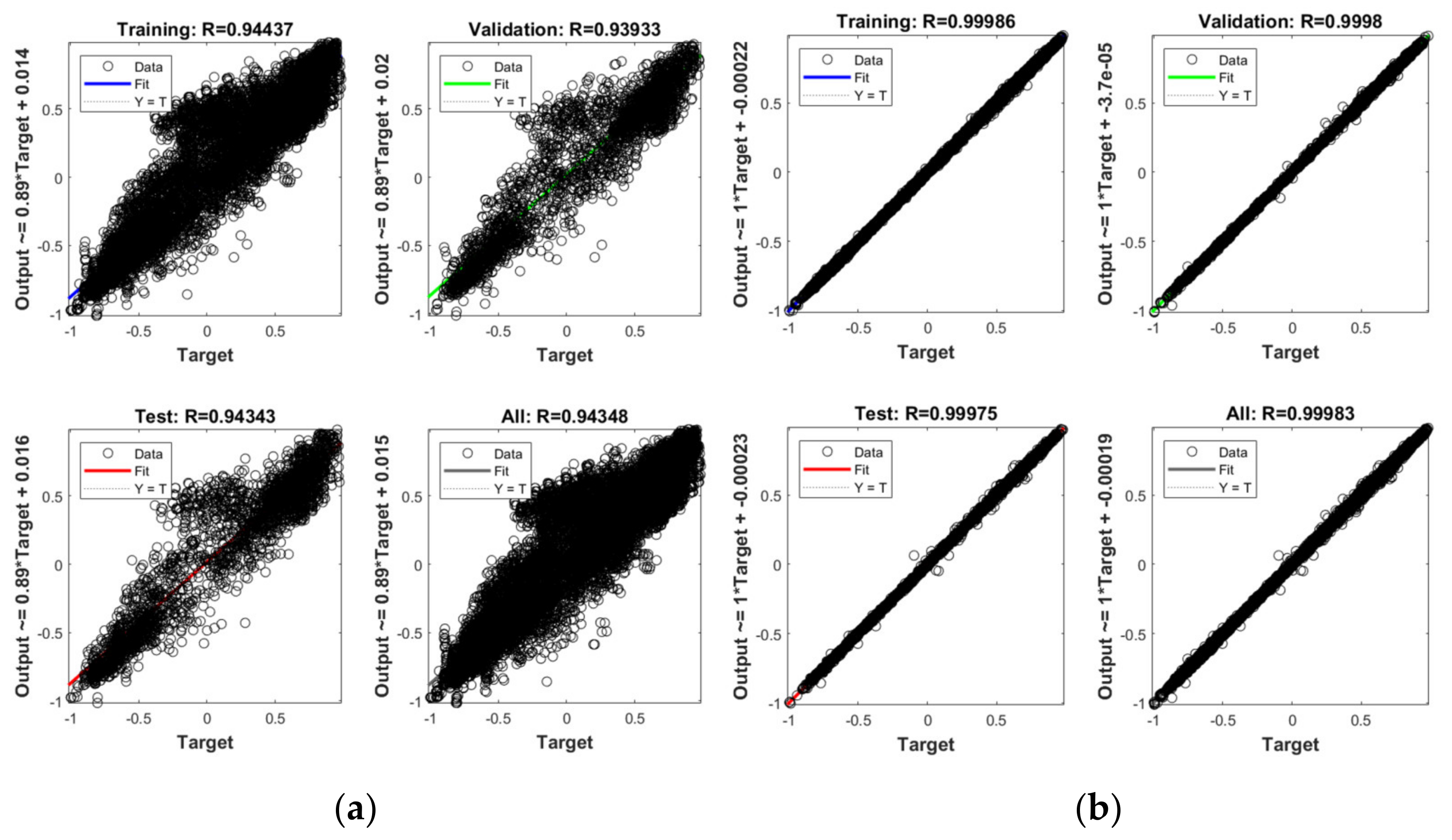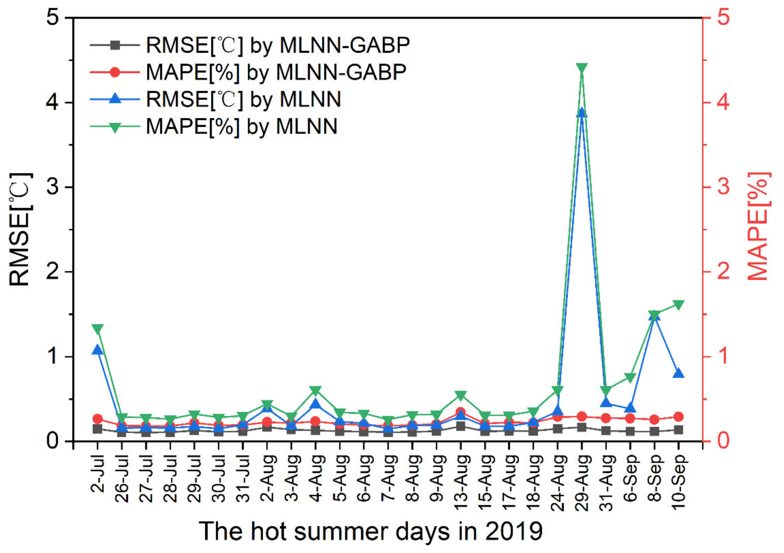[47], the backpropagation neural network model enhanced by the genetic algorithm (GA-BPNN) has greater accuracy than the BPNN method but a slower computation time. Consequently, the MLNN has higher accuracy than the one-hidden-layer FFNN. Therefore, the MLNN optimized by the GA and BP algorithm (MLNN-GABP) was selected to compare the prediction results of the MRT with the MLNN. The more accurate one could be used for sensitivity analysis.

In previous studies, numerous approaches have been presented to determine the relative relevance of ANN variables, such as the linkage weight method approach [48], the Garson algorithm approach [49], the partial derivative approach [50,51], and the sensitivity analysis approach [52]. Nonetheless, there is no unanimity due to the disparate priority assigned to the individual variables because the approach determines the relative relevance of the individual variable’s method of sensitivity analysis [53]. As a result, a proper sensitivity analysis technique is required. Chan et al. 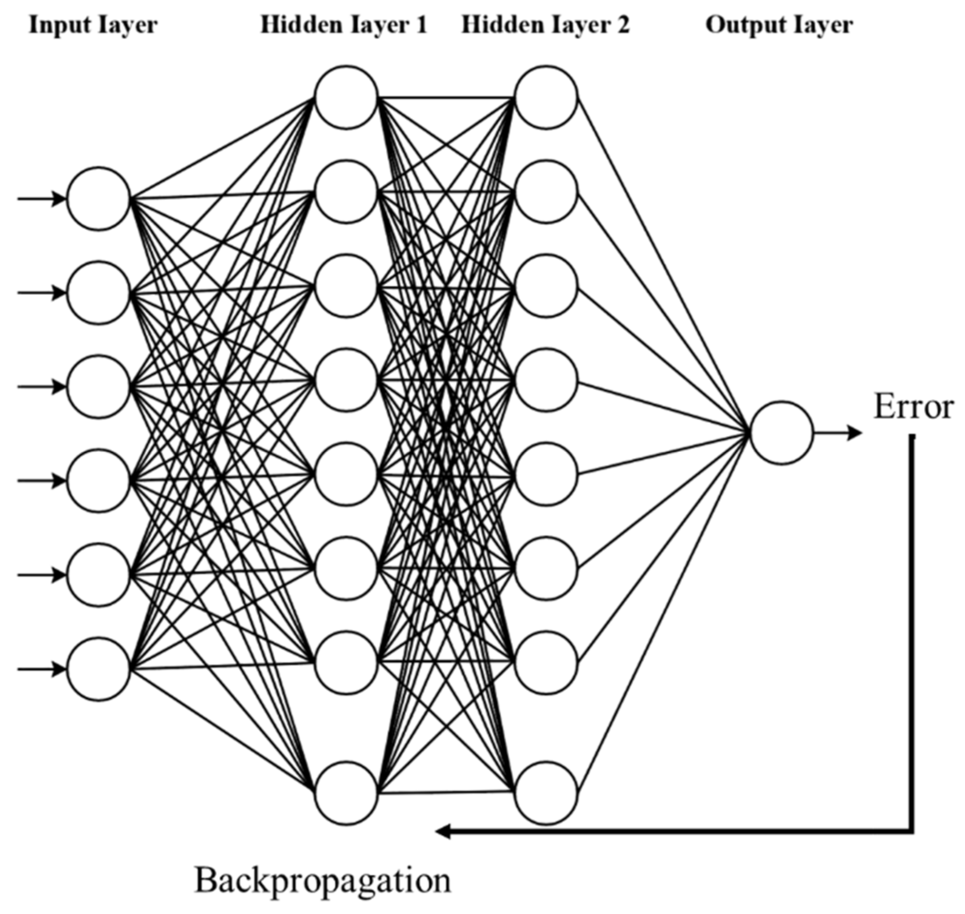[54] predicted outdoor thermal comfort using an MLNN with two hidden layers. For the summertime prediction, 12,500 training datasets were utilized and the R-value was 0.898, indicating its high accuracy. This study employs an MLNN that is capable of handling large amounts of data and achieving high accuracy and combines a biological and a weather-related metric to predict the predicted mean vote (PMV) and SET*, achieving both high prediction accuracy and ranking. According to this study, the sensitivity analysis approach was proven to be suitable for ANN. Therefore, the sensitivity analysis approach was chosen as the conference for analyzing the important variables for MRT in this study.

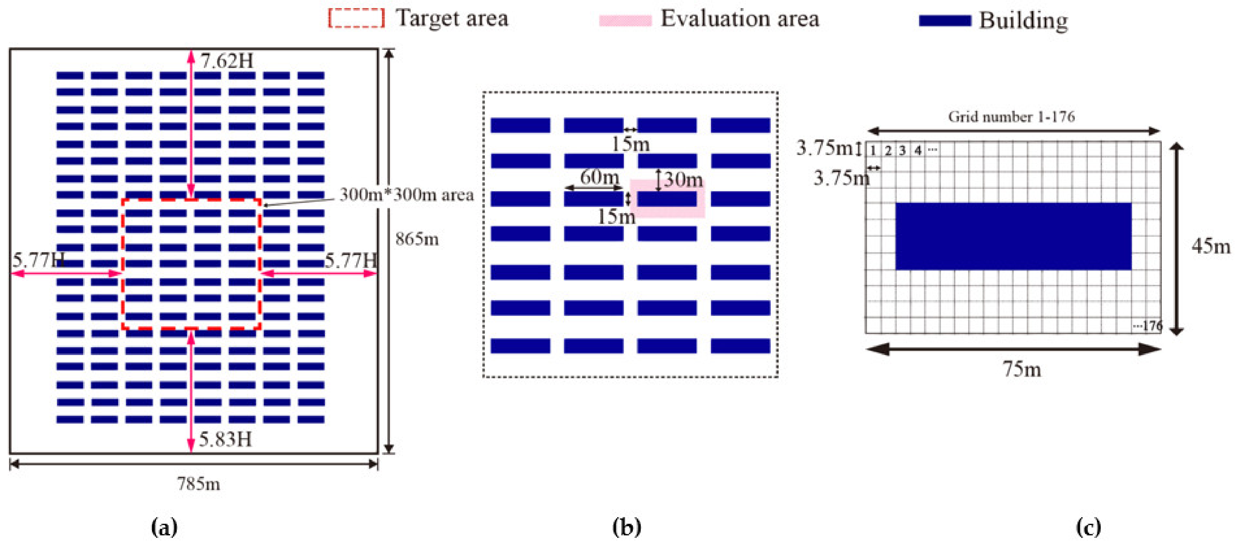
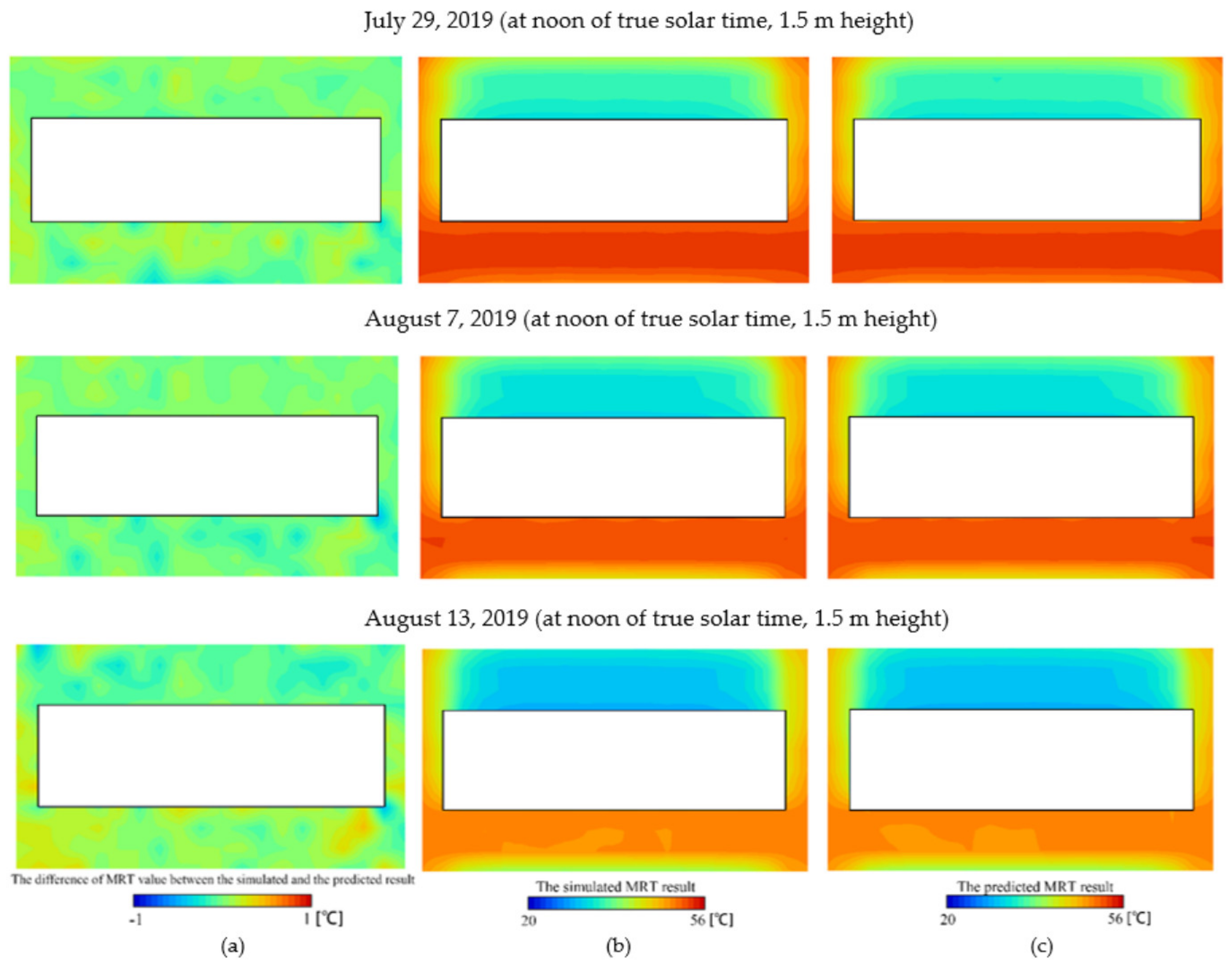
In this work, ANNs were used to predict the MRT distribution, and data were obtained every day in the summer from 2014 to 2019 in Sendai at noon true solar time (when the sun is at its greatest height and solar radiation is at its strongest). The main objective of this work is to develop MLNN-GABP models to predict the distribution of MRT at 1.5 m (pedestrian height) of the surrounding buildings. It was important to gather training and validation datasets for the ANN. The meteorological datasets from 2014 to 2018 were used as the inputs, whereas the MRT results calculated using the same weather dataset’s settings were used as the target outputs. The validation approach used the 2019 meteorological datasets as the inputs for the trained neural network and the MRT results generated under the same weather dataset’s settings as the validation outputs. The MRT prediction model was developed using a set of simplified-shape buildings in Sendai, Japan (38°16′06″ N, 140°52′10″ E).

The findings given in this paper are expected to aid in the development of a viable strategy for predicting MRT distributions without requiring extensive calculations. Urban planners and designers must provide pertinent recommendations and design measures based on optimal outdoor thermal environments.

2. Overview of This Study

In this study, the evaluation of the MRT is mostly accomplished by the collection of weather data, the development of neural networks, and sensitivity analysis. Weather data for the MRT calculation was collected from the Japan Meteorological Agency (JMA) [55]. A typical residential urban district consisting of simplified buildings in the latitude and longitude of Sendai was built in Japan, concerning previous research.

Firstly, the summer season period in Sendai must be defined, and weather data must be collected, primarily for the MRT calculations and as the input parameters to the neural network. The input for the MRT calculations and the training of the neural network will be the weather data recorded from the weather station. The expected output of this step will be the heat gain of each surface of the building during the summer season, and the MRT value around the building at a height of 1.5 m. With the trained neural network and the weather data for the whole summer period, a prediction for the MRT distribution will be made. The MRT distribution results and trained neural network will be sent for sensitivity analysis to calculate the order of importance of each input parameter to the MRT.

2.1. Weather Data Collection

Generally, the summer season is an extended period, and the weather conditions are different, including both rainy and sunny days. The different weather conditions also have a great impact on the results of the outdoor thermal environment. The three months of June, July, and August are considered summer in Japan, and the summer period differs by area. For each day, the JMA defines the days with a high temperature of over 25 °C as “summer days”, and the days with a high temperature of over 30 °C as “hot summer days”.

The JMA database was used for the MRT evaluation in this research. It is possible that the MRT readings in Sendai were impacted by factors such as global solar radiation and air temperature, as well as solar altitude, cloud cover, and the length of insolation. Predictive neural networks must be trained for at least four years in order to provide reliable findings, according to previous studies [56,57,58,59]. To train our neural networks, we used Sendai’s meteorological data for the months of July and September from 2014 to 2018. From 2014 to 2019, Sendai experienced 126 hot summer days, according to the data. Additional computations and projections were made using hourly data.

2.2. Evaluation Model Determination

Furthermore, we took into account a plan floated up by Xuan [60] to use structures in the vicinity of an 865 m (x) by 785 m (y) plot as the basis for a created region with a 16 percent coverage rate (see Figure 1). On the basis of Xuan’s prior work [60], a simpler model for residential areas was developed. The simulations in Sendai, depicted in Figure 1, were run using meteorological data and a model created with buildings facing each other (60 m (x) 15 m (y) 42 m (z)). At a z-position of 1.5 m, the simulation and assessment were carried out in the target area depicted in Figure 1b, which was 300 m (x) 300 m (y) in size. As shown in Figure 1c, the assessment area had a grid size of 3.75 m (x) 3.75 m (y). This approach has been utilized in prior research to evaluate outdoor environments [60].

An MRT calculation was done at noon true solar time in each example to calculate the 24 h heat balance. A modified urban block situated at Sendai’s latitude and longitude was used for the simulations. Additionally, the MRT was computed for summer days from 2014 to 2019 in all grids. Based on the building’s physical structure, the assessment area was split into 240 grids. Figure 1 shows the serial numbers. Building distances in the north-to-south direction were 30 m in the region investigated. The building’s surface was separated into five sections: east, west, north, south, and the roof, in order to better understand how varied orientations, affect heat gain.

3. Methodology

3.1. Heat Transfer Analysis and MRT Calculation

All surfaces in the computational domain were separated into tiny surfaces for the purpose of calculating urban surface temperatures. Direct solar radiation, sky radiation, and longwave radiation between the surface and adjacent surfaces were all analyzed for each surface. The form factor (i.e., configuration factor or view factor) was computed using the Monte Carlo technique [61,62], and the radiative heat transfer was determined using the Gebhart absorption coefficient [63]. Given that the Gebhart absorption factor varied with absorptivity as a function of shortwave and longwave radiation, we estimated these changes independently for each surface. As previously shown [64,65,66], metropolitan surface temperatures are well-recreated when the aforementioned heat exchanges are included. Figure 2 shows the structures of the ground and buildings (wall and roof), and

Table 1. Structures and thermal properties of the ground, wall, and roof.

	No. of Layers	Material for Each Layer	Thickness (mm)	Thermal Conductivity (W/(m·K))	Specific Heat per Unit Volume (kJ/m3·K)
entry 1	1	Concrete	100	1.28	1900
	2	Gravel	100	0.62	1500
	3	Soil	300	1.50	3100
entry 2	1	Exterior mortar	25	0.93	1890
	2	Aerated concrete	200	0.22	735
	3	Interior mortar	25	0.87	1785
entry 3	1	Exterior mortar	25	0.93	1890
	2	Fine stone concrete	40	1.51	2116
	3	Cement mortar	20	0.93	1890
	4	Insulation layer	30	0.036	41.4
	5	Reinforced concrete	100	1.74	2300
	6	Interior mortar	25	0.87	1785

lists the corresponding thermal properties, which are both the same as the environment of the previous study [60]. The resources were obtained by using the parameters of real building materials in the guidelines from Sendai, Japan [67].

Through the use of radiation modeling, we were able to determine the net radiation heat gain of the building’s outside surfaces. The three-dimensional multi-reflections of shortwave and longwave radiations were taken into account in order to achieve excellent prediction accuracy in this study. The Monte Carlo approach was used to compute the shape factor (also known as the configuration factor or view factor), and the Gebhart absorption factor was used to quantify the radiative heat transfer between the two surfaces. In this calculation, the radiation simulation was run every 10 min, and the output data were recorded every one hour. In the method by Nakamura [68], the human body is approximated as a rectangular prism (shown in Figure 3). Based on Nakamura’s research, previous researches [9,10,60,69] have shown that when the heat balance calculation is used, urban surface temperatures are well-reproduced. Associated with the formulas in these literatures, the same code is adopted and run in the Fortran environment to calculate the MRT in this study. Equation (1) shows the MRT calculation method from Ref. [60].

$$\sigma T_{mrt}^4={{\displaystyle \sum }}_{l=-3}^3{q}_l{\alpha }_h{c}_l+{{\displaystyle \sum }}_{l=-3}^3\left({{\displaystyle \sum }}_{j=1}^n{B}_{lj}\sigma T_j^4{c}_l\right)$$

(1)

where T_mrt is the MRT (K); c_l is the weighting factor for surface l of a rectangular prismatic human body, which is 0.024 for the top and bottom surfaces, and 0.238 for the lateral surfaces; l is the surface index of a rectangular prismatic human body, l is 1, 2, 3 or −1, −2, −3; q_l is the amount of shortwave radiation (direct, sky, and diffuse solar radiation) at surface l of a rectangular prismatic human body (W/m²); α_h is the shortwave radiation absorption coefficient for the human body, α_h = 0.5; T_j is the temperature of the surfaces surrounding the rectangular prismatic human body (K); B_lj is the Gebhart absorption coefficient, which is from the rectangular prismatic human body’s surface l to surface j; and σ is 5.67 × 10⁻⁸ W/(m²·K⁴), the Stefan–Boltzmann constant [58].

3.2. Multi-Layer Neural Network Optimized by the Backpropagation Algorithm and GA Method

In recent decades, multi-layer neural networks have become widely used. Multi-layer neural networks [70] have received a lot of attention and have been effectively used in a variety of fields, including combinatorial optimization. FFNN neural networks are used to optimize both networks, which comprise an input layer, a hidden layer, and an output layer, with the input layer’s neurons feeding parameters into the hidden nodes. When it comes to multivariate input, MLNN has an advantage over FFNN since it can be built with several hidden layers. Backpropagation is an algorithm that requires many occurrences of forward propagation in order to optimize its prediction outcomes, which was first suggested by Rumelhart [71]. A key feature of the backpropagation algorithm is the fact that the signal is transferred from the input to the output, whereas the error is conveyed from the output to the input. There are three layers in the backpropagation-optimized neural network: the input, the implicit, and the output. Using the direction propagation algorithm, the neural network may more easily achieve its learning objective by improving the connection methodology, connection weights, activation mechanism, and threshold of each neuron in each layer. The structural model is shown in Figure 4.

To keep the error within the specified range, the weights and thresholds can be corrected using the gradient descending approach. Equations (3)–(6) demonstrate the techniques for adjusting the weights of the hidden layer–output layer and the input layer–hidden layer; this is a kind of multilayer feedforward network trained using an error backpropagation algorithm that propagates errors to the weights and biases [71,72]. The error between the expected and actual outputs Ep (variance is used as an example in this study) is indicated in Equation (2).

$$Ep=\frac{1}{2}{{\displaystyle \sum }}_{j=0}^{m-1}\left(y_j-d_j\right)$$

(2)

Amount of change in weights $\Delta W$ can be calculated by:

$$\Delta W=-\eta \frac{\partial Ep}{\partial w}$$

(3)

Amount of change in thresholds $\Delta b$ can be calculated by:

$$\Delta b=-\eta \frac{\partial Ep}{\partial b}$$

(4)

Weights $b_{old}$ will be updated to $b_{new}$ by:

$$b_{new}=b_{old}-\Delta b$$

(5)

Weights $W_{old}$ will be updated to $W_{new}$ by:

$$W_{new}=W_{old}-\Delta W$$

(6)

where E represents the mean square error and outj denotes the jth neuron output. η is the learning rate parameter that determines the network’s stability and rate of network convergence; η is a constant ranging between 0 and 1 that has been set to 0.01 in this study. y, d, w, b, and Ep are predicted output, actual output, weights, biases, and variance, respectively.

The neural network optimized using the BP method is likewise limited to some extent. In the first place, the BP neural network’s application impact is greatly affected by the initial weighted value and the threshold value. This leads to the neural network being stuck in local minima during forward propagation, reducing the prediction performance; secondly, BP neural networks employ gradient descent, requiring an excessive amount of training time to optimize a complex objective function. As a result, the algorithm takes longer to reach its final output and requires more iterations. Genetic algorithm (GA) is used in this research to improve the weighted value and threshold value of the BP neural network and to create a new GA-BP neural network algorithm [45,73,74].

Steps for establishing and training a neural network model using Matlab’s GA and BP neural network prediction model are as follows:

(1)

Remove all the environment variables and normalize the data. The population sample’s weighted value and threshold value are computed using the BP neural network. y and o represent the desired and expected outputs, respectively [75],

$$F=k\left({{\displaystyle \sum }}_{i=1}^m\mathrm{abs}\left(y_i-o_i\right)\right)$$

(7)

where m, y_i, and o_i represent the number of neurons in the output layer, the ith expected value, and the ith predicted value, respectively.

(2)

Create a new feedforward neural network, with a learning rate of 0.05, and set training parameters such as the factor of momentum, minimum root mean square error for the training, and the prediction of the BP network.

(3)

Initialize genetic algorithm parameters. Confirm the number of iterations to be 50, the population size to be 10, the crossover probability to be Pc = 0.75, and mutation probability to be Pm = 0.25.

(4)

Initialize the population. A random population of chromosomes is used to record the best and average fitness of the chromosomes in each generation of the iteration. Individuals with outstanding fitness are chosen to carry on to the next generation. In this research, the roulette approach is used to determine fi, which reflects the fitness of the individual i and can be computed by Equation (8),

$$f_i=k/F_i$$

(8)

$p_i$ denotes the likelihood of an individual i being selected; it may be determined using Equation (9),

$$p_i=\frac{f_i}{{{\displaystyle \sum }}_{i=1}^N{f}_i}$$

(9)

where $F_i$ is the fitness function of the individual i; k is the selectivity coefficient.

(5)

Solve the best initial threshold value and weighted value through iteration. Through a process of selecting, crossing, and variating the population, it is possible to determine the population’s minimum and maximum fitness chromosomes and their relative positions, and then use those values to replace the previous generations’ worst individuals and their corresponding fitness values. This process continues until the maximum number of iterations has been reached. During the calculating procedure, the GA algorithm uses the entity code. In this study, the real number crossing method is used, where a_xi represents the bit i of the xth chromosome, which can be calculated by Equation (10)

$$a_{xi}=a_{xi}\left(1-b\right)+a_{yi}b$$

(10)

$a_{yi}$ represents the bit i of the yth chromosome, it can be calculated by Equation (11),

$$a_{yi}=a_{yi}\left(1-b\right)+a_{xi}b$$

(11)

where b represents the random number (0 ≤ b ≤ 1), respectively.

Based on the formula below, there is a definite possibility that when one individual is selected, certain genes are transformed into other alleles:

$$a_{ij}=\left\{\begin{array}{c}{a}_{ij}+\left(a_{ij}-a_{\max }\right)·f\left(g\right),r>0.5\\ a_{ij}+\left(a_{\min }-a_{ij}\right)·f\left(g\right),r\le 0.5\end{array}\right.$$

(12)

Among Equation (12), the iteration formula is shown below:

$$f\left(g\right)=r_2{\left(1-\frac{g}{G_{\max }}\right)}^2$$

(13)

where a_max, a_min, r₂, g, G_max, and r represent the upper bound of the gene a_ij, the lower bound of the gene a_ij, random number, iteration times, maximum times, and random number (0 ≤ r ≤ 1), respectively.

(6)

In order to train and predict the GA-BP network, the BP network should be assigned the ideal initial weighted value and the threshold value.

3.3. Sensitivity Analysis Approach

When Chan et al. [54] combined the predictions of neural networks in order to derive the order of importance for various types of input parameters, they used a sensitivity analysis method to demonstrate how to account for both the influence of weather parameters and also other related parameters on the outdoor thermal environment. Thus, the same sensitivity analysis technique is used in this research to determine the relative relevance of various kinds of input parameters, yielding the same conclusion as in the prior study. The approach employed in this investigation is as follows [76]. The following formula was used to obtain the percentage band for the input variables:

$$\frac{X{i}_{\max }-X{i}_{\min }}{100}$$

(14)

X_i stands for the ith input variable. In the ANN model, a 4% band (+2% and −2%) of each input variable was trained. Before training, the values of all the input variables become Y_i + 2% X_i and Y_i − 2% X_i. After that, the differences (Δyi) between Y_i + 2% X_i and Y_i − 2% X_i were calculated. For each variable, the index of the order of importance (I_Ri) for each variable was determined by:

$$\frac{\mathsf{\Delta }yi}{Y{i}_{\max }-Y{i}_{\min }}$$

(15)

After that, the input variables were classified according to their significance. As shown in the References [76,77,78,79] section, a succession of ANNs was employed to highlight the significance of certain components in a particular order. The employment of a collection of ANNs has been found to be promising in terms of producing relatively consistent results while avoiding the instability problem associated with a single optimum network [80]. As a consequence, rather than using a single ideal network, this research made use of collections of neural networks. The relevance of the input variables was assessed using sets of trained neural networks. For additional examination, a total of twenty of the strongest neural models from winter and summer were selected. The R and MSE values from the validation datasets were utilized to assess the formed ANN model’s prediction performance. Following that, a sensitivity analysis was conducted of all neural networks, and a ranking of each neural network’s order of significance was obtained.

4. The Structure of the Neural Network

4.1. Selecting the Input Parameters

Correlation coefficients were calculated between each pair of input variables using weather data from JMA that could affect MRT, including solar direction, solar altitude, air temperature at noon true solar time, daily average air temperature, insolation time, minimum air temperature, global solar radiation, maximum air temperature, and cloud cover. The related parameters in each grid that might affect the MRT and that were proven in previous studies were selected for the correlation coefficient analysis. Among them, the sky view factor of each grid, sunshine duration before noon true solar time, and the shadow ration in each grid at noon true solar time are related to the morphology of urban space. These three parameters can be calculated in SketchUp and its plug-ins. The ground surface temperature has been shown to impact the MRT at the pedestrian level, and this may be determined using the previously described heat balance analysis. The majority of the correlation coefficients between the input variables are shown in

Table 2. Correlation coefficients between the input variables.

	X1	X2	X3	X4	X5	X6	X7	X8	X9	X10	X11	X12	X13
X1	1
X2	0.740	1
X3	0.280	0.036	1
X4	0.342	0.051	0.604	1
X5	0.471	0.078	0.421	0.931	1
X6	0.356	0.068	0.608	0.907	0.940	1
X7	0.557	0.099	0.104	0.741	0.907	0.743	1
X8	0.192	0.153	0.946	0.689	0.515	0.691	0.221	1
X9	0.096	0.073	0.796	0.403	0.245	0.415	0.036	0.884	1
X10	0.182	0.079	0.116	0.049	0.118	0.105	0.084	0.031	0.059	1
X11	0.221	0.147	0.173	0.289	0.214	0.326	0.450	0.038	0.176	0.032	1
X12	0.178	0.143	0.116	0.004	0.071	0.059	0.151	0.157	0.018	0.031	0.046	1
X13	0.096	0.116	0.004	0.071	0.059	0.151	0.157	0.018	0.132	0.031	0.046	0.074	1

X1: solar altitude, X2: solar direction, X3: insolation time, X4: air temperature at noon true solar time, X5: daily average air temperature, X6: maximum air temperature, X7: minimum air temperature, X8: global solar radiation, X9: cloud cover, X10: the sky view factor of each grid, X11: sunshine duration before noon true solar time, X12: the shadow ration in each grid at noon true solar time, X13: ground surface temperature.

. There are significant collinearities detected, with correlation values greater than 0.8 [54]. A strong correlation between the input variables may result in the ANN models being overfit and introducing many redundancies.

Several factors that may have had an impact on the MRT between 2014 and 2019 were studied for correlation and are shown in Table 2. The average air temperature and the average air temperature at noon true solar time, as well as the maximum and minimum air temperatures, all have strong relationships, as shown in Table 2. Because of this, there were two viable options: one required picking just the average air temperature, and the other required selecting both the air temperature at noon true solar time as well as the lowest air temperature. The second choice was selected due to the need for as many diverse input variables as was reasonably possible. Moreover, as the length of insolation and the amount of cloud cover were substantially connected with solar radiation and with one another, global solar radiation was selected as the input parameter for the training process. As a consequence, there is little association between the grid metrics associated with each grid point and the meteorological data.

Accordingly, average air temperature, maximum air temperature, insolation duration, and cloud cover were removed and replaced with minimum air temperature, air temperature at noon true solar time, and global solar radiation. Therefore, solar altitude, solar direction, air temperature at noon, minimum air temperature, global solar radiation, the sky view factor of each grid, sunshine duration before noon true solar time, the shadow ration in each grid at noon true solar time, and ground surface temperature can be used for training neural networks as the input parameters.

4.2. The Structure of MLNN-GABP

According to the findings of this study, the database was initially divided into two groups: one containing the weather and building-related parameters from 2014 to 2018 as well as the MRT of each grid from their simulation results as the training dataset (which contained 80 percent of the data), and another containing the weather and building-related parameters from 2019 along with the MRT of each grid from their simulation results as the validation dataset (which contained 20 percent of the data). In the training set, three subsets are used to determine performance: 60 percent is used for training, 20 percent is used for validation, and 20 percent is used for testing. Both the validation and test datasets are constructed in such a way that overfitting on the training data is avoided, resulting in a more realistic accuracy of the test data. It seems that the neural network was effectively trained when the training set, validation set, and test set all provide appropriate training results, suggesting that it was successfully trained.

As a result of a broad variety of training environments and a wide range of data, a technique for normalizing the data is needed. Oversaturation, which occurs when bigger datasets cover smaller datasets, slows down mechanical learning, hence standardized data is often utilized to train data in a consistent range. For predicting outdoor thermal comfort, the following standardization approach was used in the literature, and the current research makes reference to that method by applying the formula:

$$NV=\frac{N{V}_{\max }-N{V}_{\min }}{V_{\max }-V_{\min }}\times \left(V-V_{\min }\right)+N{V}_{\min }$$

(16)

where NV is the input or output normalized vector; NV_max = 1; NV_min = −1; V is the input or output data; V_max is the maximum of the input or output data; and V_min is the minimum of the input or output data.

The structure of MLNN-GABP is shown in

Table 3. ANN model structure.

Prediction Period	Random Validation
Input layer	Number of neurons: 9
Weather parameters	Solar altitude
	Minimum air temperature
	Global solar radiation
	Solar direction
	Air temperature at noon true solar time
The related parameters in each mesh	Sky view factor of each grid
	Sunshine duration before noon of the true solar time
	Shadow ration in each grid at noon true solar time
	Ground surface temperature
Hidden layer	Number of neurons: 7–19
Number of training cases	20,064
Number of validation cases	4400
Output layer	Number of neurons: 1 (MRT)

. The validation dataset comprises 25 hot summer days in 2019 (a total of 25 days times 176 grids = 4400 validation data) and is used to validate the validation set. In the training step, all 176 hot summer days from 2014 to 2018 were selected as the training dataset (a total of 114 days times 176 grids = 20,064 validation data), and the ratio of the training set, test set, and validation set is 3:1:1 in the training step. In the test step, the ratio of the training set, test set, and validation set is 3:1:1. The input parameters in each grid are comprise mostly weather parameters, with a total of nine input parameters in total for each grid. The number of hidden layers was determined by the application of Equation (17). At a height of 1.5 m, the output parameter is the mean solar time (MRT) at midday true solar time for each grid. Table 3 lists the variables that are used to construct the input layer, hidden layer, and output layer, respectively. The algorithms for the neural networks, genetic algorithms, and backpropagation algorithms are all implemented in MATLAB using the code that was developed for each method. The multilayer feedforward neural networks that we used for this investigation were created using MATLAB-based software, and the ANN models were tested using the results.

$$2\times \sqrt{N_{input}}+N_{output}\le N_{hidden}\le 2\times N_{input}+1$$

(17)

where N_input is the number of input neurons, N_output is the number of output neurons, and N_hidden is the number of hidden neurons.

To validate the suggested technique, we compared the MLNN and MLNN-GABP outcomes. The root mean square error (RMSE) and mean absolute percentage error (MAPE) were employed to assess these three models’ predictive accuracy. The root mean square error (RMSE) values were determined using:

$$MSE=\sqrt{\frac{1}{n}{{\displaystyle \sum }}_{i=1}^n{\left(x_i\left(t\right)-y_i\left(t\right)\right)}^2}$$

(18)

and the MAPE values were calculated using

$$MAPE=\frac{1}{n}{{\displaystyle \sum }}_{i=1}^n\left|\frac{x_i\left(t\right)-y_i\left(t\right)}{x_i\left(t\right)}\right|\times 100\%$$

(19)

where x_i(t) and y_i(t) represent the ith actual and predicted values at time t, respectively.

MAPE was employed to assess predictive performance in the previous research: MAPE is smaller than 10% (excellent), MAPE is between 10% and 20% (acceptable), MAPE is between 20% and 50% (fair), and MAPE is smaller than 50% (bad).

5. Validation Results

5.1. Validating the Input Parameters and Determining Hidden Layers

By putting the training through its paces, and the validation and test sets of ANNS, the prediction performance was tested. As shown in

Table 4. A summary of R-values of the subset of the training dataset and validation dataset after adding additional variables.

Added Variable	R-Values of the Training Set	R-Values of the Validation Set	R-Values of the Test Set
Weather parameters	0.6732	0.6542	0.6643
+ Sky view factor of each grid,	0.7556	0.7589	0.8013
+ Sunshine duration before noon true solar time,	0.8059	0.8011	0.8213
+ Shadow ration in each grid at noon true solar time	0.93478	0.9365	0.9372
+ Ground surface temperature	0.99986	0.9998	0.9997

below, increasing a parameter implies that the trained neural network is not overfit and that the training parameters are reasonable. After incorporating the weather, shadow, sunshine, and sky view factors, the prediction accuracy was significantly improved, and after including the ground surface temperature in each grid, the prediction results were even more accurate, with an R-value greater than 0.999, indicating extremely high accuracy.

The R-values of the training, validation, and test sets with varied hidden layer counts, as well as the predicted RMSE and MAPE, were evaluated in this study. For the purposes of validating and comparing the prediction performance with the various hidden layer count,

Table 5. The parameters of ANNs used for determining the hidden layer.

No	ANN Structure	R-Value			RMSE	MAPE
		Training Set	Validation Set	Test Set
1	9-15-12-1	0.99986	0.9998	0.99975	0.13	0.23%
2	9-13-11-1	0.99752	0.99864	0.99741	0.15	0.28%
3	9-16-12-1	0.99652	0.99698	0.99701	0.17	0.34%
4	9-17-12-1	0.99521	0.99523	0.99710	0.19	0.45%
5	9-15-10-1	0.99465	0.99501	0.99601	0.21	0.48%
6	9-16-11-1	0.99425	0.99465	0.99532	0.24	0.57%

shows the R-values, RMSE, and MAPE in the six MLNN-GABP structures with the smallest RMSE. Structured with 9 input layers, 15 hidden layers, 12 hidden layers, and 1 output layer, it indicates very high prediction accuracy, with an RMSE of 0.13, and a MAPE of 0.23%.

5.2. Comparison of MLNN-GABP and MLNN

To evaluate the prediction performance of the GA and BPs’ effect on neural network training, Figure 5 compares the prediction results of MLNN with the prediction results of MLNN-GABP, and also shows the prediction performance of the training dataset, validation set, and test set. The R-value of the training dataset does not differ significantly from the R-values of the validation and test sets, indicating that the training performed is not overfitting. According to the training results in this study, both neural networks have a good training structure (R-value greater than 0.90), but the results of the MLNN-GABP optimization are obviously more accurate than MLNN. When the neural network without the GA and BP algorithm has a greater error at some points and the accuracy of the training results is improved by the GA and BP algorithm, there are smaller errors in individual samples.

5.3. The Prediction Results of MRT Distribution

These findings are depicted in Figure 6, which shows that the MRT values predicted by MLNN-GABP are exceptionally accurate in hot summers. The RMSE and MAPE values of 0.13 °C and 0.23%, respectively, show that the predicted and calculated values almost coincide, suggesting an extraordinarily high degree of accuracy. Using RMSE and MAPE, the predicted results are compared by days in Figure 7. As can be observed, the RMSE for all predicted days is less than 0.2 and the MAPE is less than 0.3%, indicating daily extremely high prediction accuracies, with 13 August having the highest error and 7 August having the lowest error. MRT distribution plots were generated for the three days with the highest and lowest errors, and those closest to the average error, as shown in Figure 8. When the predicted and calculated values were compared, just a 1 °C discrepancy was found, and the distribution plot results were identical.

5.4. Order of Importance of the Input Variables

Sensitivity analysis was used to determine the thermal comfort evaluation for the MRT input factors. As illustrated in Figure 9, the positive axis indicates that the input variable is positively correlated with the output variable, whereas the negative axis indicates that the input variable is negatively correlated with the MRT distribution, and the larger the value, the greater the influence of that input variable on the MRT distribution. Thus, the order of importance for the input variables can be determined accordingly. The analysis of this importance rating can provide direction for future architectural design and environmental shaping. To begin, it was discovered that surface temperature and global radiation are the primary contributing elements, whereas the sky coefficient has a significant effect on building shape, and the building shadow is adversely connected with the MRT. Therefore, the proposed optimization measures for these four parameters will be more effective in future architectural and urban design.

6. Conclusions

Using meteorological data and artificial neural networks (ANNs), we developed a unique technique of MRT prediction for a reduced block construction model. In addition, we compared the results of the ANN predictions with the results of the heat balance analysis simulations conducted during the years 2014–2018, as well as for the year 2019, which were not included in the training datasets but were acquired from other sources. The following are the findings and ramifications of this study.

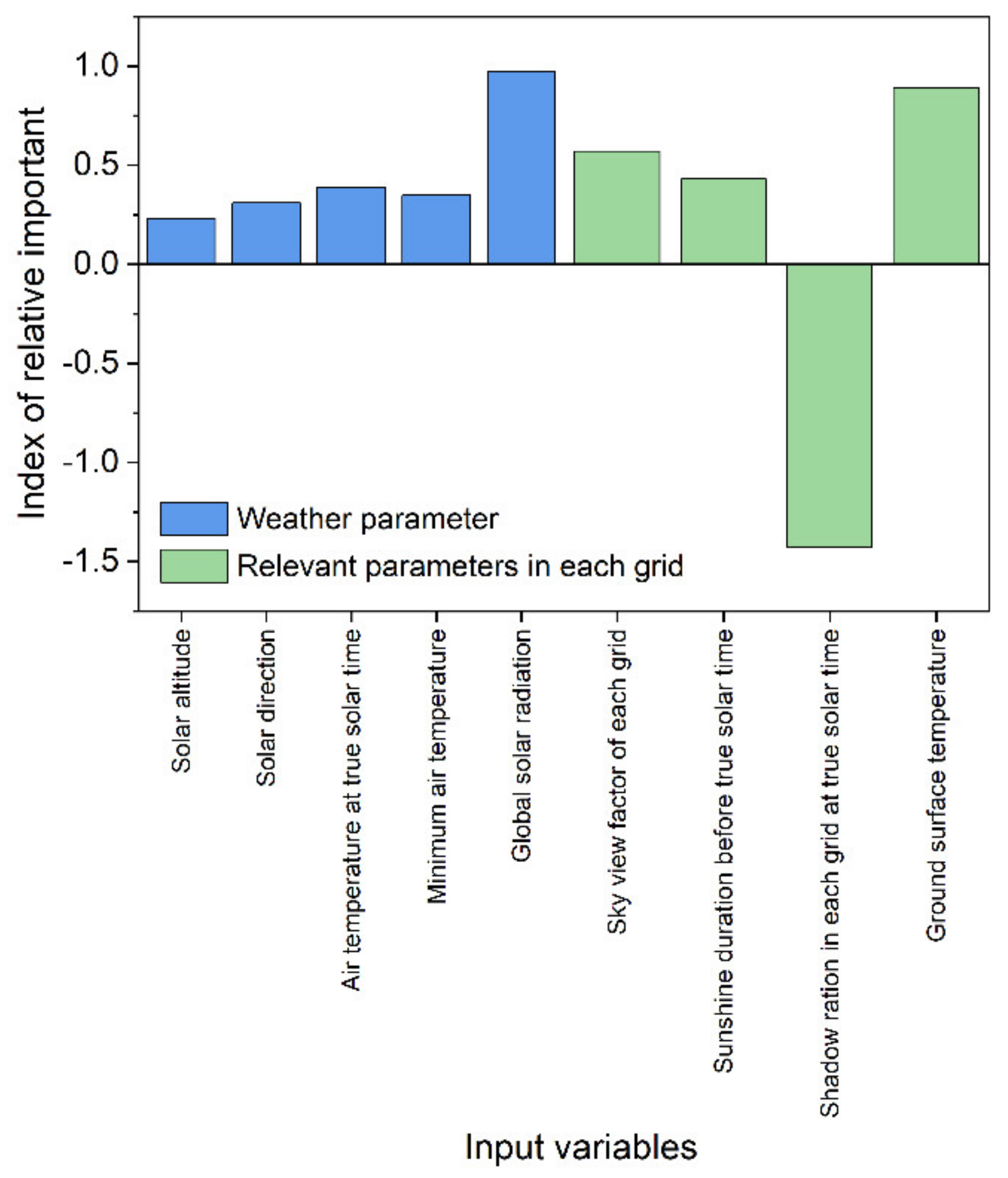
• We selected the weather parameters (solar altitude, solar direction, air temperature at noon true solar time, minimum air temperature, and global solar radiation) and the related parameters in each mesh (the sky view factor of each grid, sunshine duration before noon true solar time, the shadow ration in each grid at noon true solar time, and ground surface temperature) as the input parameters for the training datasets, which proved suitable for the MRT distribution prediction under a particular building form.
• The article optimized the MLNN using a BP algorithm and GA; the optimization results indicated that the GA and BP algorithm have some effect on the results. The neural network without optimization produces more deviant prediction values, whereas the optimized neural network produces more stable prediction values when dealing with a large matrix.
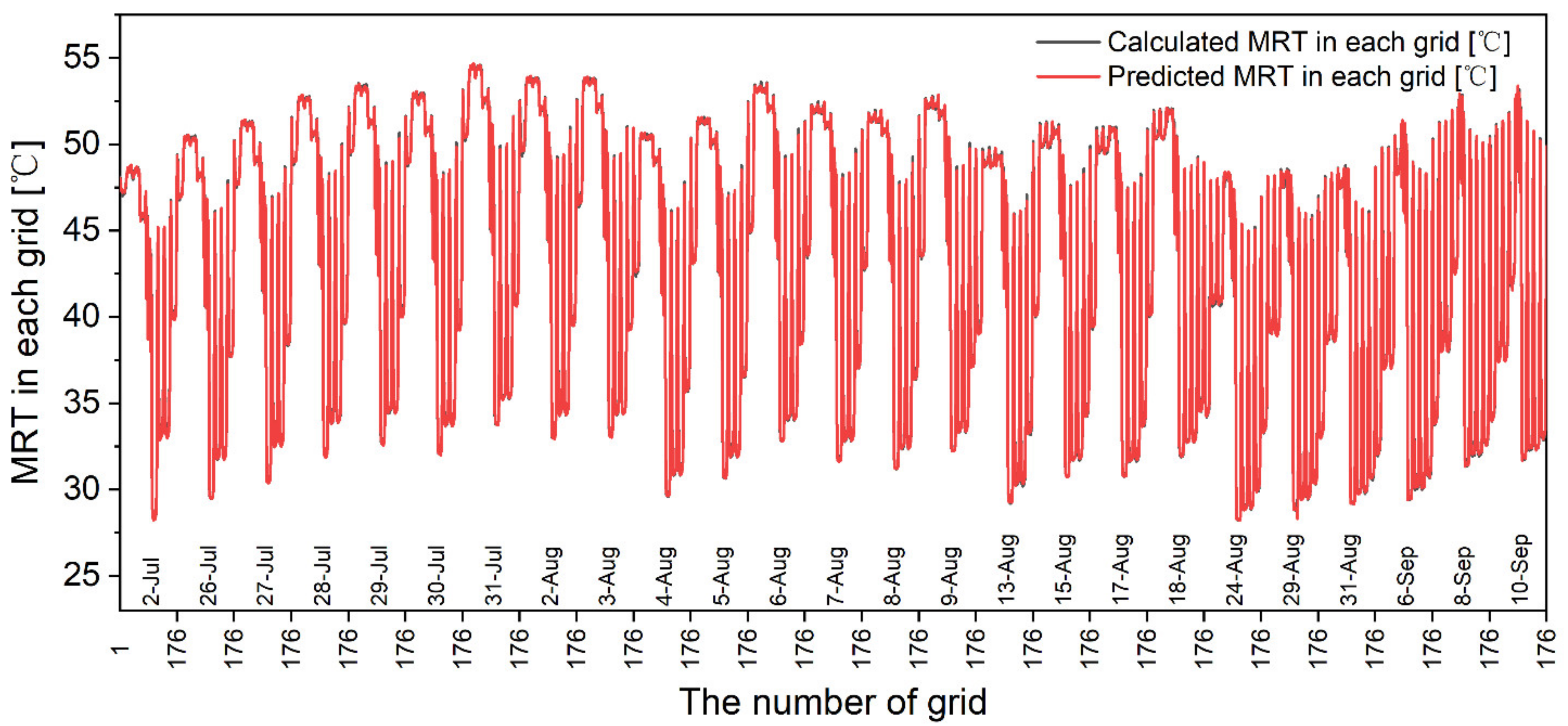
• An MLNN-GABP model was created to derive the MRT values from the weather variables during a specified period. After five years of training, it is possible to forecast the MRT distribution for the following year. The prediction results are extremely accurate, and a comparison of the MRT distribution plots reveals that they are consistent. As a result, the influence of this input parameter on the output can be analyzed using sensitivity analysis, and a relationship between the grid-related indicators and the MRT distribution can be determined.

Still, the proposed method has limitations. First, the MRT was only predicted using meteorology data for Sendai (38°16′06″ N, 140°52′10″ E), considering simplified building shapes, and the method only proposes an algorithm; further verifications are expected for realistic urban blocks in future works. It has not been validated in this study whether this method is applicable if other parameters are considered, such as trees, water, etc. Meanwhile, it is also important to consider wind patterns and non-realistic building arrangements. Therefore, further analysis will need to be conducted in subsequent research to address this issue. Second, the developed prediction method was only confirmed to predict the simulated results; it should be validated if this method can predict the MRT in real buildings. Finally, although this prediction has very high accuracy, it requires a large number of training datasets. Therefore, it would be very difficult to obtain five-year training data if this method were scheduled to be used in a real building environment and measured in the future.

7. Future Work

First, we will validate whether the method is accurate after considering trees, water bodies, grasses, etc. For this purpose, we will select a real building and build a similar model (including vegetation, water bodies, etc.), and adjust the input parameters of the grid accordingly. We will compare the accuracy of the method in predicting the MRT values and the order of importance for the input parameters in each grid for different building heights and different distances between the buildings to extend the applicability of the method. Second, if this method can accurately predict the distribution of the MRT around the model as the actual building, then we will combine this method with real measurements, where the surface temperature can be measured by drones, and weather data and other grid-related data can be calculated by measurements or software simulations. This is because MRT is more difficult to measure in real measurements, though the wind velocity, humidity, and air temperature can be more easily measured. The MRT distribution around the building can be quickly predicted by this method, and even the further prediction of the SET* distribution can be tried later. Finally, for a large number of training datasets, we will try to combine PCA and K-means and other methods in the future to remove weather conditions that are too similar, which helps to reduce the computation time and keep accurate prediction results while retaining high prediction accuracy. After completing these steps, we will be able to combine neural networks to analyze outdoor thermal environments very quickly and accurately, which will provide a reference for designers to propose strategies to adapt to urban warming and to improve outdoor thermal environments more efficiently.

References

1. UN. World Urbanization Prospects: The 2018 Revision; UN DESA: New York, NY, USA, 2019. [Google Scholar] [CrossRef] [Green Version]
2. Arnfield, A.J. Two decades of urban climate research: A review of turbulence, exchanges of energy and water, and the urban heat island. Int. J. Clim. 2003, 23, 1–26. [Google Scholar] [CrossRef]
3. Oke, T.R. Boundary Layer Climates; Routledge: London, UK, 1987. [Google Scholar]
4. Oke, T.R. Street design and urban canopy layer climate. Energy Build. 1988, 11, 103–113. [Google Scholar] [CrossRef]
5. Masson-Delmotte, V.; Zhai, P.; Pörtner, H.O.; Masmoudi, S. An IPCC Special Report on the Impacts of Global Warming of 1.5 °C Above Pre-Industrial Levels and Related Global Greenhouse Gas Emission Pathways; IPCC-World Meteorological Organization: Geneva, Switzerland, 2018. [Google Scholar]
6. National Institute for Environmental Studies. Bulletin Report on Heatstroke Patients. 2012. Available online: http://www.nies.go.jp/gaiyo/archiv/risk8/ (accessed on 4 December 2017).
7. Yamamoto, M.; Kasai, M.; Okaze, T.; Hanaoka, K.; Mochida, A. Analysis of climatic factors leading to future summer heatstroke risk changes in Tokyo and Sendai based on dynamical downscaling of pseudo global warming data using WRF. J. Wind Eng. Ind. Aerodyn. 2018, 183, 187–197. [Google Scholar] [CrossRef]
8. Chen, L.; Ng, E.Y.Y. Outdoor thermal comfort and outdoor activities: A review of research in the past decade. Cities 2012, 29, 118–125. [Google Scholar] [CrossRef]
9. Yumino, S.; Uchida, T.; Sasaki, K.; Kobayashi, H.; Mochida, A. Total assessment for various environmentally conscious techniques from three perspectives: Mitigation of global warming, mitigation of UHIs, and adaptation to urban warming. Sustain. Cities Soc. 2015, 19, 236–249. [Google Scholar] [CrossRef]
10. Yoshida, S.; Murakami, S.; Ooka, R.; Mochida, A.; Tominaga, Y. CFD prediction of thermal comfort in microscale wind climate. In Proceedings of the Third International Symposium on Computational Wind Engineering, Birmingham, UK, 4–7 September 2000. [Google Scholar]
11. Sasaki, K.; Mayer, H.; Mochida, A.; Uchida, M.; Tonouchi, T. Field measurement of thermal comfort in outdoor locations—Comparison of SET* and PET based on questionnaire survey. In Proceedings of the Seventh International Conference on Urban Climate, Yokohama, Japan, 29 June–3 July 2009. [Google Scholar]
12. Koch, W. Relationship between Air Temperature and Mean Radiant Temperature in Thermal Comfort. Nature 1962, 196, 587. [Google Scholar] [CrossRef] [PubMed]
13. Masmoudi, S.; Mazouz, S. Relation of geometry, vegetation and thermal comfort around buildings in urban settings, the case of hot arid regions. Energy Build. 2004, 36, 710–719. [Google Scholar] [CrossRef]
14. Thorsson, S.; Rocklöv, J.; Konarska, J.; Lindberg, F.; Holmer, B.; Dousset, B.; Rayner, D. Mean radiant temperature—A predictor of heat related mortality. Urban Clim. 2014, 10, 332–345. [Google Scholar] [CrossRef]
15. Ali-Toudert, F.; Mayer, H. Numerical study on the effects of aspect ratio and orientation of an urban street canyon on outdoor thermal comfort in hot and dry climate. Build. Environ. 2006, 41, 94–108. [Google Scholar] [CrossRef]
16. Yahia, M.W.; Johansson, E. Influence of urban planning regulations on the microclimate in a hot dry climate: The example of Damascus, Syria. J. Hous. Built Environ. 2012, 28, 51–65. [Google Scholar] [CrossRef]
17. Mayer, H.; Höppe, P. Thermal comfort of man in different urban environments. Theor. Appl. Climatol. 1987, 38, 43–49. [Google Scholar] [CrossRef]
18. Cohen, S.; Palatchi, Y.; Palatchi, D.P.; Shashua-Bar, L.; Lukyanov, V.; Yaakov, Y.; Matzarakis, A.; Tanny, J.; Potchter, O. Mean radiant temperature in urban canyons from solar calculations, climate and surface properties—Theory, validation and ‘Mr.T’ software. Build. Environ. 2020, 178, 106927. [Google Scholar] [CrossRef]
19. Pang, Z.; Niu, F.; O’Neill, Z. Solar radiation prediction using recurrent neural network and artificial neural network: A case study with comparisons. Renew. Energy 2020, 156, 279–289. [Google Scholar] [CrossRef]
20. Xue, X. Prediction of daily diffuse solar radiation using artificial neural networks. Int. J. Hydrogen Energy 2017, 42, 28214–28221. [Google Scholar] [CrossRef]
21. Koca, A.; Oztop, H.F.; Varol, Y.; Koca, G.O. Estimation of solar radiation using artificial neural networks with different input parameters for Mediterranean region of Anatolia in Turkey. Expert Syst. Appl. 2011, 38, 8756–8762. [Google Scholar] [CrossRef]
22. Yadav, A.K.; Chandel, S. Solar radiation prediction using Artificial Neural Network techniques: A review. Renew. Sustain. Energy Rev. 2014, 33, 772–781. [Google Scholar] [CrossRef]
23. Anis, S.; Jamil, B.; Ansari, A.; Bellos, E. Generalized models for estimation of global solar radiation based on sunshine duration and detailed comparison with the existing: A case study for India. Sustain. Energy Technol. Assess. 2018, 31, 179–198. [Google Scholar] [CrossRef]
24. Lindberg, F.; Thorsson, S.; Rayner, D.; Lau, K. The impact of urban planning strategies on heat stress in a climate-change perspective. Sustain. Cities Soc. 2016, 25, 1–12. [Google Scholar] [CrossRef]
25. Tan, C.L.; Wong, N.H.; Jusuf, S.K. Outdoor mean radiant temperature estimation in the tropical urban environment. Build. Environ. 2013, 64, 118–129. [Google Scholar] [CrossRef]
26. Manavvi, S.; Rajasekar, E. Estimating outdoor mean radiant temperature in a humid subtropical climate. Build. Environ. 2020, 171, 106658. [Google Scholar] [CrossRef]
27. Andrić, I.; Pina, A.; Ferrao, P.; Fournier, J.; Lacarrière, B.; Le Corre, O. Assessing the feasibility of using the heat demand-outdoor temperature function for a long-term district heat demand forecast. Energy Procedia 2017, 116, 460–469. [Google Scholar] [CrossRef]
28. Dogan, T.; Kastner, P.; Mermelstein, R. Surfer: A fast simulation algorithm to predict surface temperatures and mean radiant temperatures in large urban models. Build. Environ. 2021, 196, 107762. [Google Scholar] [CrossRef]
29. Lai, P.-Y.; Koh, J.H.; Koh, W.S.; Liu, H. Effectively modeling surface temperature and evaluating mean radiant temperature in tropical outdoor industrial environments. Build. Environ. 2020, 169, 106227. [Google Scholar] [CrossRef]
30. Roman, N.D.; Bre, F.; Fachinotti, V.D.; Lamberts, R. Application and characterization of metamodels based on artificial neural networks for building performance simulation: A systematic review. Energy Build. 2020, 217, 109972. [Google Scholar] [CrossRef]
31. Zhao, H.-X.; Magoulès, F. A review on the prediction of building energy consumption. Renew. Sustain. Energy Rev. 2012, 16, 3586–3592. [Google Scholar] [CrossRef]
32. Van Gelder, L.; Das, P.; Janssen, H.; Roels, S. Comparative study of metamodelling techniques in building energy simulation: Guidelines for practitioners. Simul. Model. Pract. Theory 2014, 49, 245–257. [Google Scholar] [CrossRef]
33. Østergård, T.; Jensen, R.L.; Maagaard, S.E. A comparison of six metamodeling techniques applied to building performance simulations. Appl. Energy 2018, 211, 89–103. [Google Scholar] [CrossRef]
34. Yuan, J.; Nian, V.; Su, B.; Meng, Q. A simultaneous calibration and parameter ranking method for building energy models. Appl. Energy 2017, 206, 657–666. [Google Scholar] [CrossRef]
35. Romani, Z.; Draoui, A.; Allard, F. Metamodeling the heating and cooling energy needs and simultaneous building envelope optimization for low energy building design in Morocco. Energy Build. 2015, 102, 139–148. [Google Scholar] [CrossRef]
36. Rackes, A.; Melo, A.P.; Lamberts, R. Naturally comfortable and sustainable: Informed design guidance and performance labeling for passive commercial buildings in hot climates. Appl. Energy 2016, 174, 256–274. [Google Scholar] [CrossRef]
37. Cheng, M.-Y.; Cao, M.-T. Accurately predicting building energy performance using evolutionary multivariate adaptive regression splines. Appl. Soft Comput. 2014, 22, 178–188. [Google Scholar] [CrossRef]
38. Kumar, R.; Aggarwal, R.; Sharma, J. Energy analysis of a building using artificial neural network: A review. Energy Build. 2013, 65, 352–358. [Google Scholar] [CrossRef]
39. Wang, W.; Li, M.; Hassanien, R.H.E.; Ji, M.E.; Feng, Z. Optimization of thermal performance of the parabolic trough solar collector systems based on GA-BP neural network model. Int. J. Green Energy 2017, 14, 819–830. [Google Scholar] [CrossRef]
40. Mohandes, S.R.; Zhang, X.; Mahdiyar, A. A comprehensive review on the application of artificial neural networks in building energy analysis. Neurocomputing 2019, 340, 55–75. [Google Scholar] [CrossRef]
41. Zarra, T.; Galang, M.G., Jr.; Ballesteros, F.; Belgiorno, V.; Naddeo, V. Environmental odour management by artificial neural network—A review. Environ. Int. 2019, 133, 105189. [Google Scholar] [CrossRef]
42. Fu, X.; Li, S.; Michael, F.; Donald, C.W.; Eduardo, A. Training recurrent neural networks with the Levenberg–Marquardt algorithm for optimal control of a grid-connected converter. IEEE Trans. Neural Netw. Learn. Syst. 2014, 26, 1900–1912. [Google Scholar] [CrossRef] [Green Version]
43. Magoulast, G.; Vrahatis, M.; Androulakis, G. On the alleviation of the problem of local minima in back-propagation. Nonlinear Anal. Theory 1997, 30, 4545–4550. [Google Scholar] [CrossRef]
44. Kolhe, M.; Lin, T.C.; Maunuksela, J. GA-ANN for Short-Term Wind Energy Prediction. In Proceedings of the 2011 Asia-Pacific Power and Energy Engineering Conference, Wuhan, China, 25–28 March 2011; pp. 1–6. [Google Scholar]
45. Ata, R. RETRACTED: Artificial neural networks applications in wind energy systems: A review. Renew. Sustain. Energy Rev. 2015, 49, 534–562. [Google Scholar] [CrossRef]
46. Mba, L.; Meukam, P.; Kemajou, A. Application of artificial neural network for predicting hourly indoor air temperature and relative humidity in modern building in humid region. Energy Build. 2016, 121, 32–42. [Google Scholar] [CrossRef]
47. Zhu, C.; Zhang, J.; Liu, Y.; Ma, D.; Li, M.; Xiang, B. Comparison of GA-BP and PSO-BP neural network models with initial BP model for rainfall-induced landslides risk assessment in regional scale: A case study in Sichuan. China. Nat. Hazards 2020, 100, 173–204. [Google Scholar] [CrossRef]
48. Olden, J.D.; Joy, M.K.; Death, R.G. An accurate comparison of methods for quantifying variable importance in artificial neural networks using simulated data. Ecol. Model. 2004, 178, 389–397. [Google Scholar] [CrossRef]
49. Garson, G.D. Interpreting neural-network connections. Artif. Intell. Expert 1991, 6, 47–51. [Google Scholar] [CrossRef]
50. Dimopoulos, Y.; Bourret, P.; Lek, S. Use of some sensitivity criteria for choosing networks with good generalization ability. Neural Process. Lett. 1995, 2, 1–4. [Google Scholar] [CrossRef]
51. Shojaeefard, M.H.; Akbari, M.; Tahani, M.; Farhani, F. Sensitivity Analysis of the Artificial Neural Network Outputs in Friction Stir Lap Joining of Aluminum to Brass. Adv. Mater. Sci. Eng. 2013, 2013, 574914. [Google Scholar] [CrossRef] [Green Version]
52. Scardi, M.; Harding, L.W. Developing an empirical model of phytoplankton primary production: A neural network case study. Ecol. Model. 1999, 120, 213–223. [Google Scholar] [CrossRef]
53. De Oña, J.; Garrido, C. Extracting the contribution of independent variables in neural network models: A new approach to handle instability. Neural Comput. Appl. 2014, 25, 859–869. [Google Scholar] [CrossRef]
54. Chan, S.Y.; Chau, C.K. Development of artificial neural network models for predicting thermal comfort evaluation in urban parks in summer and winter. Build. Environ. 2019, 164, 106364. [Google Scholar] [CrossRef]
55. Japan Meteorological Agency. 2020. Available online: https://www.jma.go.jp/jma/indexe.html (accessed on 31 October 2020).
56. Jiang, Y. Prediction of monthly mean daily diffuse solar radiation using artificial neural networks and comparison with other empirical models. Energy Policy 2008, 36, 3833–3837. [Google Scholar] [CrossRef]
57. Alam, S.; Kaushik, S.; Garg, S. Assessment of diffuse solar energy under general sky condition using artificial neural network. Appl. Energy 2009, 86, 554–564. [Google Scholar] [CrossRef]
58. Jiang, Y. Computation of monthly mean daily global solar radiation in China using artificial neural networks and comparison with other empirical models. Energy 2009, 34, 1276–1283. [Google Scholar] [CrossRef]
59. Elmas, Ç. Artificial Neural Networks (Theory, Architecture, Education, Application); Seçkin Publication House: Ankara, Turkey, 2003. [Google Scholar]
60. Xuan, Y.; Yang, G.; Li, Q.; Mochida, A. Outdoor thermal environment for different urban forms under summer conditions. Build. Simul. 2016, 9, 281–296. [Google Scholar] [CrossRef]
61. Howell, J.R.; Perlmutter, M. Monte Carlo Solution of Thermal Transfer through Radiant Media Between Gray Walls. J. Heat Transf. 1964, 86, 116–122. [Google Scholar] [CrossRef]
62. Omori, T.; Yang, J.; Kato, S.; Murakami, S. Radiative Heat Transfer Analysis Method for Coupled Simulation of Convection and Radiation in Large-Scale and Complicated Enclosures: Part 2—Analysis of Thermal Environment around Human Body Model with Realistic Shape and Size. Trans. Soc. Heat. Air-Condition. Sanitary Eng. Jpn. 2003, 28, 93–102. [Google Scholar]
63. Gebhart, B. A new method for calculating radiant exchanges. ASHRAE Trans. 1959, 65, 321–332. [Google Scholar]
64. Chen, H.; Ooka, R.; Harayama, K.; Kato, S.; Li, X. Study on outdoor thermal environment of apartment block in Shenzhen, China with coupled simulation of convection, radiation and conduction. Energy Build. 2004, 36, 1247–1258. [Google Scholar] [CrossRef]
65. Huang, H.; Ooka, R.; Kato, S. Urban thermal environment measurements and numerical simulation for an actual complex urban area covering a large district heating and cooling system in summer. Atmos. Environ. 2005, 39, 6362–6375. [Google Scholar] [CrossRef]
66. Mochida, A.; Yoshino, H.; Miyauchi, S.; Mitamura, T. Total analysis of cooling effects of cross-ventilation affected by microclimate around a building. Sol. Energy 2006, 80, 371–382. [Google Scholar] [CrossRef]
67. 平成25年住宅・建築物の省エネルギー基準解説書編集委員会編: 平成25年省エネルギー基準に準拠した算定・判断の方法及び解説. Available online: https://www.kenken.go.jp/becc/house_h25.html (accessed on 20 April 2020).
68. Nakamura, Y. Expression method of the radiant field on a human body in buildings and urban spaces. J. Archit. Plan. Environ. Eng. 1987, 376, 29–35. [Google Scholar] [CrossRef] [Green Version]
69. Yoshida, S.; Mochida, A. Evaluation of effects of windows installed with near-infrared rays retro-reflective film on thermal environment in outdoor spaces using CFD analysis coupled with radiant computation. Build. Simul. 2018, 11, 1053–1066. [Google Scholar] [CrossRef]
70. Hornik, K.; Stinchcombe, M.; White, H. Multilayer feedforward networks are universal approximators. Neural Netw. 1989, 2, 359–366. [Google Scholar] [CrossRef]
71. Rumelhart, D.E.; Hinton, G.E.; Williams, R.J. Learning representations by back-propagating errors. Nature 1986, 323, 533–536. [Google Scholar] [CrossRef]
72. Wang, Z.; Liu, Y.; He, D.; Chan, S. Intrusion detection methods based on integrated deep learning model. Comput. Secur. 2021, 103, 102177. [Google Scholar] [CrossRef]
73. Song, S.; Xiong, X.; Wu, X.; Xue, Z. Modeling the SOFC by BP neural network algorithm. Int. J. Hydrogen Energy 2021, 46, 20065–20077. [Google Scholar] [CrossRef]
74. Xing, Y.; Li, F. Research on the influence of hidden layers on the prediction accuracy of GA-BP neural network. J. Phys. Conf. Ser. 2020, 1486, 022010. [Google Scholar] [CrossRef]
75. Jianying, F.; Bianyu, Y.; Xin, L.; Dong, T.; Weisong, M. Evaluation on risks of sustainable supply chain based on optimized BP neural networks in fresh grape industry. Comput. Electron. Agric. 2021, 183, 105988. [Google Scholar] [CrossRef]
76. Bayat, H.; Ebrahimi, E.; Ersahin, S.; Hepper, E.N.; Singh, D.N.; Amer, A.-M.M.; Yukselen-Aksoy, Y. Corrigendum to Analyzing the effect of various soil properties on the estimation of soil specific surface area by different methods. Appl. Clay Sci. 2016, 124-125, 271. [Google Scholar] [CrossRef]
77. Cao, M.; Qiao, P. Neural network committee-based sensitivity analysis strategy for geotechnical engineering problems. Neural Comput. Appl. 2007, 17, 509–519. [Google Scholar] [CrossRef]
78. Hadzima-Nyarko, M.; Nyarko, E.K.; Morić, D. A neural network based modelling and sensitivity analysis of damage ratio coefficient. Expert Syst. Appl. 2011, 38, 13405–13413. [Google Scholar] [CrossRef]
79. Pentoś, K. The methods of extracting the contribution of variables in artificial neural network models—Comparison of inherent instability. Comput. Electron. Agric. 2016, 127, 141–146. [Google Scholar] [CrossRef]
80. Zhou, Q.; Hub, P.; Ritter, M.R.; Swenson, S.D.; Argounovaa, S.; Epstein, A.L.; Markland, F.S. Molecular Cloning and Functional Expression of Contortrostatin, a Homodimeric Disintegrin from Southern Copperhead Snake Venom. Arch. Biochem. Biophys. 2000, 375, 278–288. [Google Scholar] [CrossRef]
Figure 1. Simplified model of the residential area located in Sendai: (a) Residential area; (b) target area; (c) evaluation area and grid number.
Buildings 12 00513 g001
Figure 2. Structures of the ground and buildings (wall and roof): (a) Building wall; (b) Roof; (c) Ground.
Buildings 12 00513 g002
Figure 3. Rectangular prismatic human body.
Buildings 12 00513 g003
Figure 4. The structure of multilayer neural network optimized by backpropagation algorithm.
Buildings 12 00513 g004
Figure 5. The training results of different neural networks: (a) MLNN; (b) MLNN-GABP.
Buildings 12 00513 g005
Figure 6. The validation results on the MRT distribution in each mesh on hot summer days in 2019.
Buildings 12 00513 g006
Figure 7. The RMSE and MAPE of the prediction results in each mesh on hot summer days in 2019.
Buildings 12 00513 g007
Figure 8. Comparison of the predicted results and calculated results: (a) The difference between the simulated results and the predicted results; (b) the simulated results; and (c) predicted results by the MLNN-GABP neural network.
Buildings 12 00513 g008
Figure 9. Order of importance of the input variables for hot summer days.
Buildings 12 00513 g009