Post-Disaster Temporary Shelters Distribution after a Large-Scale Disaster: An Integrated Model

Abstract

This paper develops an integrated model for the distribution of post-disaster temporary shelters after a large-scale disaster. The proposed model clusters impacted areas using an Adaptive Neuro-Fuzzy Inference System (ANFIS) method and then prioritizes the points of clusters by affecting factors on the route reliability using a permanent matrix. The model’s objectives are to minimize the maximum service time, maximize the route reliability and minimize the unmet demand. In the case of ground relief, the possibility of a breakdown in the vehicle is considered. Due to the disaster’s uncertain nature, the demands of impacted areas are considered in the form of fuzzy numbers, and then the equivalent crisp counterpart of the non-deterministic is made by Jimenez’s method. Since the developed model is multi-objective, the Non-dominated Sorting Genetic Algorithm (NSGA-II) and Multi-Objective Firefly Algorithm (MOFA) are applied to find efficient solutions. The results confirm higher accuracy and lower computational time of the proposed MOFA. The findings of this study can contribute to the growing body of knowledge about disaster management strategies and have implications for critical decision-makers involved in post-disaster response projects. Furthermore, this study provides valuable information for national decision-makers in countries with limited experience with disasters and where the destructive consequences of disasters on the built environment are increasing.

1. Introduction

There is a growing consensus that disasters do not occur naturally but rather due to poor planning [1]. The rising frequency and severity of disasters pose a severe threat to human society and the built environment [2], resulting in large-scale population displacement. Almost 42 million people were forced to abandon their homes due to natural hazards in 2010 alone [3]. After a disaster, a large number of people are left without a place to live, and one of the most obvious consequences is damage to housing [4]. Damaged houses require extensive repair and reconstruction. As a result, providing emergency shelter to those in need takes precedence over all other actions. Communities that have been affected by natural disasters can resume their daily routines in temporary shelter units, which provide them with the necessary protection while they await the completion of the reconstruction process [5]. Prefabricated units and other forms of temporary shelters are designed for short-term occupants after a disaster event to serve the displaced communities [6,7]. However, many logistical issues can arise when providing temporary shelters for displaced people in the immediate aftermath of natural disasters.

The literature on disaster risk management in construction and the built environment has received insufficient attention [8]. Following a disaster, the construction industry is often called upon to provide various crucial services, including temporary shelters in the immediate aftermath and permanent shelter reconstruction [5,9]. A lack of planning and administration can exacerbate the difficulties inherent in reconstruction projects, which can be further compounded by international aid organizations’ lack of expertise in dealing with such matters [10].

This article focuses on the response phase and the problem of the distribution of post-disaster temporary shelters after a large-scale disaster. In this problem, we encounter impacted areas where the vehicles should serve them and then return to the shelter’s warehouse with the lowest possible cost. In times of crisis, we strive to reduce total travel time to provide shelters faster for the impacted people. The number of warehouses (e.g., without, single warehouse, and multiple warehouses) in a transportation system, the number of periods (e.g., single and multiple), the type of fleet (e.g., heterogeneous and non-heterogeneous), and the type of transportation (e.g., single and multiple) are all influencing factors on a distribution system’s agility and performance. The presence of an open or closed vehicle routing problem can also significantly impact the speed and security of distribution operations.

Designers of distribution networks of post-disaster temporary shelters are generally looking for quick and equitable distribution [11]. In order to achieve this goal, it is crucial to identify and cluster areas that have similar needs and features. ANFIS can cluster the impacted areas [12]. In a crisis, having a secure transportation network is critical, and considering secure and safe routes appears to be a very reasonable action [13]. These issues prevent unanticipated delays, ensure the safety of drivers and relief personnel, allow for the safe transport of vehicles, and ensure the timely arrival of temporary shelters. As a result, this can be accomplished by weighing the impacted areas concerning some influencing criteria on the road reliability. It is also possible to specify the priority of each impacted point using various Multi-Criteria Decision-Making (MCDM) methods [14,15]. Because of the nature of the disasters and a lack of reliable information, there is uncertainty in demand, supply, transportation time, etc.

On the other hand, the distribution of temporary shelters and equipment will be complex because infrastructure and routes may be disrupted. Disorders are expected during the response phase, following a crisis and the implementation of distribution operations [16]. These disruptions are sometimes the result of unexpected events, such as vehicle breakdowns. As a result, some impacted areas cannot receive services from that vehicle, and even active vehicles, due to driver shift exchange or completion of the defined time, cannot deliver the remaining shelters of the broken-down vehicle to the impacted areas, leaving them unserved. As a result, there is a shortage in the distribution system. This shortage (i.e., unmet demand) is minimised in this study. The primary objective of this study is to develop an integrated model and an advanced computational approach to assist decision-makers in addressing the challenges associated with the distribution of post-disaster temporary shelters that many communities face following the occurrence of a destructive large-scale disaster. The specific research objectives of this study are as follows:

• Analyzing initial requirements to develop an integrated model for distributing temporary shelters following a large-scale disaster.
• Developing an integrated model to aid in distributing temporary shelters following a large-scale destructive disaster.

This paper proposes a mathematical multi-objective model (i.e., minimisation of the maximum serving time, maximisation of route reliability, and minimisation of unmet demand) for a disrupted VRP in which impacted areas are first clustered (by applying the ANFIS). These points are then prioritised based on the factors that influence reliability (applying a graph theoretical-matrix permanent method). Diverse vehicles and depots in multi-mode (i.e., ground and air) transportation are used in temporary shelter distribution operations during the disaster response phase.

The remainder of the paper is organised as follows: Section 2 contains a review of the literature. Section 3 explains and formulates the proposed model, including clustering impacted areas using ANFIS, reliable route selection, modelling, and the proposed augmented $\mathsf{\epsilon }$-constraint method. Section 4 and Section 5 present two multi-objective metaheuristics algorithms and analyses their results. Finally, the conclusion in Section 6 brings the paper to a close.

2. Literature Review

This section investigates several streams of previous related research in the literature and research gaps in two separate sub-sections.

2.1. Disaster Risk Management

Disaster management aims to reduce or avoid the potential losses from hazards, assure prompt and appropriate assistance to disaster victims, and achieve rapid and effective recovery [17,18]. Disaster Risk Management (DRM) consists of processes for designing, implementing, and evaluating strategies, policies, and measures to improve our understanding of disaster risk, promote disaster risk reduction and transfer and stimulate a continuous improvement in disaster mitigation, preparedness, response and recovery activities [19,20]. Disaster risk management comprises four activities that are often considered as part of ongoing and interconnected processes [19]. These four activities are mitigation, preparedness, response and recovery [19], which are described by The United Nations International Strategy for Disaster Reduction (UNISDR) as follows:

• Mitigation: “The lessening or minimizing of the adverse impacts of a hazardous event./The adverse impacts of hazards, in particular natural hazards, often cannot be prevented fully, but their scale or severity can be substantially lessened by various strategies and actions. Mitigation measures include engineering techniques and hazard-resistant construction as well as improved environmental and social policies and public awareness [21].”;
• Preparedness: “The knowledge and capacities developed by governments, response and recovery organizations, communities and individuals to effectively anticipate, respond to and recover from the impacts of likely, imminent or current disasters [21].”;
• Response: “Actions taken directly before, during or immediately after a disaster in order to save lives, reduce health impacts, ensure public safety and meet the basic subsistence needs of the people affected. /Disaster response is predominantly focused on immediate and short-term needs and is sometimes called disaster relief. Effective, efficient and timely response relies on disaster risk-informed preparedness measures, including the development of the response capacities of individuals, communities, organizations, countries and the international community [21].”;
• Recovery: “The restoring or improving of livelihoods and health, as well as economic, physical, social, cultural and environmental assets, systems and activities, of a disaster-affected community or society, aligning with the principles of sustainable development and “build back better”, to avoid or reduce future disaster risk [21].”

Although disaster risk management has evolved into much more than what was earlier envisaged, many parts, such as distribution routing planning of shelters or temporary housing, have received less attention.

2.2. Disaster Distribution Routing Planning

The first studies in this field were conducted by Haghani and Oh [22] and Haghani [23], who proposed a multi-objective model for commodity distribution in which a transportation network with various fleet types distributes various types of goods. Until 2010, studies focused on other routing parameters such as multi-mode distribution, multiple products, clustering, and multi-objectivity. Özdamar et al. [24] developed a model with multiple relief modes for distributing multi-type products over time. They used a Lagrangian relaxation method to solve the model. Despite the critical importance of instant response in a routeing problem and goods distribution, particularly in times of emergency, a few researchers considered a model that would meet this requirement.

Dondo and Cerdá [25] considered demand point clustering in non-crisis fields and assigned heterogeneous vehicles to each cluster. He et al. [26] proposed a vehicle routeing model under non-crisis conditions using a heuristic algorithm and designing a goods distribution network by clustering demand points using a balanced k-means algorithm to distribute goods to demand points. However, the approach used to cluster demand points in crisis conditions (i.e., damaged points) in the ANFIS network structure is fuzzy c-means, which is not found in any research with this content. From 2010 to early 2016, papers took on a new shape, and previously unaddressed efficient and effective routeing factors were incorporated into mathematical models. Vehicle heterogeneity, multi-mode and multi-period distribution operations, uncertainty, disruption, reliability, and other efficient factors have been considered in these studies. Although reliability is critical in ensuring relief goods’ safe and timely delivery, it has received little attention in studies. Some researchers have recently considered and applied this concept to the design of distribution networks.

Vitoriano et al. [27] proposed a goal programming model for relief distribution that considered reliability and route safety factors, with relief goods delivered to heterogeneous vehicles from multiple depots to damaged areas. Torabi et al. [28] also proposed a location-routing model at a conference, in which infrastructure disruption (e.g., roads) was considered, and relief goods from multiple depots were delivered to affected areas to maximise route reliability. Hamedi et al. [29] developed a multi multi-depot multi-objective function and designed a road disruption product distribution network. Nasiri and ShisheGar [30], on the other hand, proposed a model for rapid and secure response after a crisis in which damaged points are prioritised based on affecting factors on route reliability. Heterogeneous vehicles are in charge of providing relief batches to damaged points.

Among the papers reviewed, the subject of distribution network disruption has been studied under normal conditions rather than in times of crisis. According to these studies, disruption can occur in a variety of ways. For example, road breakdowns, facility and equipment failures, vehicle breakdowns, and bad weather conditions cause problems in the humanitarian relief logistics goods distribution system, which can be fixed by using different methods and reprogramming. Although vehicle breakdowns are a significant disruption in the routeing and distribution problem, only a few researchers addressed this issue in the literature. In the non-crisis situations, for example, Wang et al. [31] introduced vehicle breakdown as a disruption in serving demand points and assumed that in the case of vehicle breakdown throughout goods distribution, other vehicles could do their serving duties before finishing their serving operation, leaving no demand points unsatisfied. Mu and Eglese [32], and Mamasis et al. [33] proposed disrupted routeing models in separate papers, in which the vehicle fails during goods distribution and the absence of the immobilised vehicle is covered by rerouting of other vehicles, and its corresponding demand points are satisfied, and thus the cost of delay is reduced. Gharib et al. [34] presented a three-stage integrated model for a cluster-based emergency vehicle routing problem in disaster considering reliability. Current study is the extended version of this study. Jiang et al. [35] introduced the problem of delayed distribution and decreased service level to customers (in the case of vehicle breakdown) and the concept of disruption management in a VRP and presented a prioritising method for customer serving in a time period.

This study tries to develop a multi-objective mathematical model for the response phase, in which land and air fleet are deployed in a temporary shelter distribution system. Multiple depots were considered as distribution centres, and impacted areas were clustered using the ANFIS method to speed up distribution operations. Damaged points in each cluster are prioritised by affecting factors on reliability, using an integration method of graph theory-MCDM-permanent matrix, to ensure perfect and on-time delivery to these areas. The probability of breakdown has been considered in the cluster related to ground relief, and we are looking to minimise the shortage of temporary shelters at the impacted areas caused by this disruption and try to reduce the current disruption, based on produced scenarios, by minimising unmet demand (i.e., undelivered goods to the damaged points).

3. Proposed Framework for a Disaster Response Strategy

The following three steps outline the procedure for developing the model in this study. Step 1 involves the clustering and prioritisation of impacted areas, while Step 2 involves presenting all stages of the mathematical model design. After that, two multi-objective metaheuristic algorithms are presented to solve the problem. This is illustrated schematically in Figure 1.

3.1. Clustering Impacted Areas Using ANFIS

By clustering the impacted areas, response strategies for sending shelters to impacted areas can be accelerated. Therefore, this study uses Adaptive Neuro-Fuzzy Inference System (ANFIS), which has shown acceptable performance in clustering problems [36]. ANFIS combines the FIS with a backpropagation algorithm used for neural network training [37]. This inference-based structure has three components depending on the selection of fuzzy rules, database (i.e., membership determination), and argument or inference on rules and obtaining the appropriate output [38]. Chu [39] proposed a neural learning method with an adaption for the FIS modelling process for information learning (i.e., ANFIS), which is the best generator for FIS. 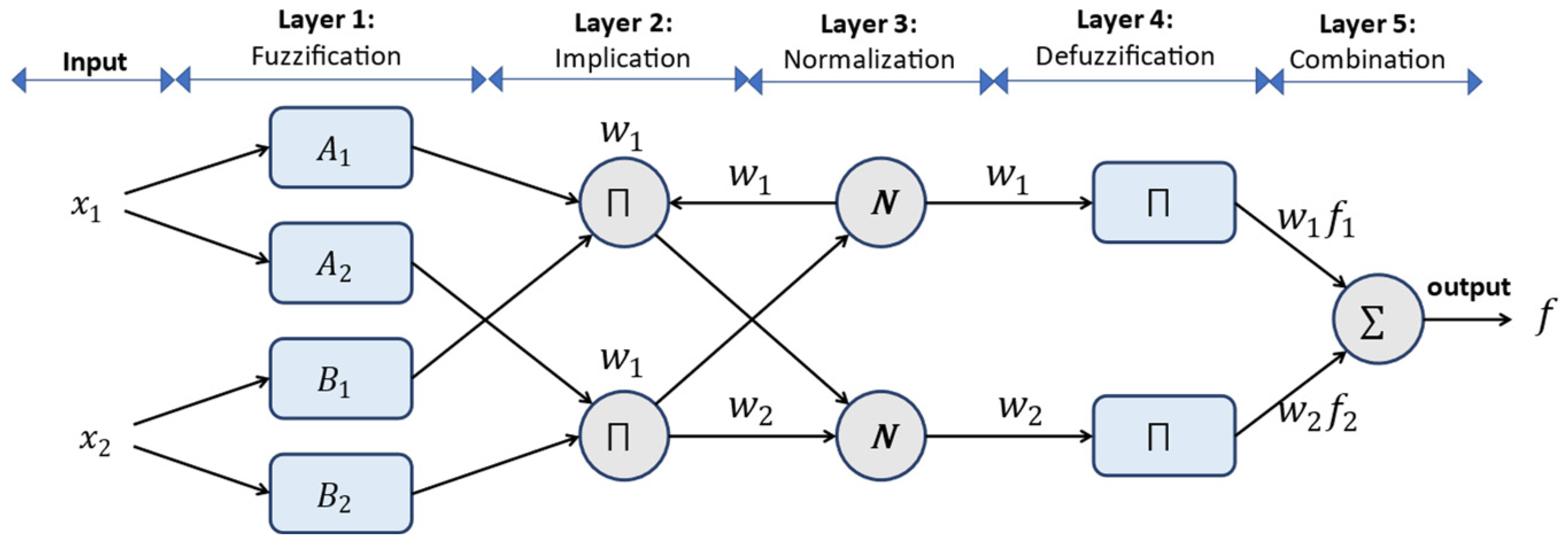This structure is a multi-layer feed-forward network that uses neural network learning algorithms and fuzzy logic for mapping an input space to an output space, and by embedding this adapted network in the Sugeno fuzzy model, the model learning is facilitated [40]. The general structure of this method is shown in Figure 2.

In this structure, the adapted nodes (i.e., squares) are the set of adjustable parameters, while fixed nodes (i.e., circles) present constant parameters in the model. The previous layer’s output is used as input of the next layer [40]. According to Figure 2, two input variables $x_1$ and $x_1$ and output y are considered to define two rules as follows [41]

• Rule 1: If $x_1$ is ${\mathcal{A}}_1 \mathrm{and} x_2 \mathrm{is} {\mathcal{B}}_1 \mathrm{then} {\mathcal{Y}}_1={𝓅}_1{x}_1+{𝓆}_1{x}_2+{𝓇}_1$
• Rule 2: If $x_1$ is ${\mathcal{A}}_2 \mathrm{and} x_2 \mathrm{is} {\mathcal{B}}_2 \mathrm{then} {\mathcal{Y}}_2={𝓅}_2{x}_1+{𝓆}_2{x}_2+{𝓇}_2$

In the current paper, for example, the first rule states that if the road slope is low, the weather is normal, the crisis severity is high, and the road risk is moderate, then the intended damaged point belongs to cluster 1. If the road slope is moderate, the weather is normal, the crisis severity is very high, and the road risk is moderate, the intended damaged point falls into cluster 2, and so on. The ANFIS determines the output value using five layers.

Layer 1. This layer maps input variables $x_1$ and $x_2$ to fuzzy sets $\mathcal{A}=\left\{{\mathcal{A}}_1, {\mathcal{A}}_2, {\mathcal{B}}_1, {\mathcal{B}}_2\right\}$ through the fuzzification method (A and B are verbal tags, like high and low). Each node in this layer is an adapted node with n function nodes that the bell or Gaussian membership function can produce. In fact, each node is used for one membership function [41].

$$\mathcal{O}=\mu \left(x\right)$$

(1)

Layer 2. After generating membership functions, each node in this layer is a fixed (i.e., constant) node, and the output is the multiplication of all inputted signals that represent the Firing Strength of each fuzzy rule. In this layer, after the combination of fuzzy sets of each input, the Firing Strength is applied, and determination of output is used from $\prod -\mathrm{norm}$ operator or the fuzzy letter “and” [40].

$$\mathcal{O}={𝓌}_i=\mu \left(x_1\right)\prod {\mu }_{\left(x_2\right)}$$

(2)

Layer 3. Each node in this layer is a fixed layer that calculates the Firing Strength rate for each rule and divides it by all rules’ Firing Strengths. Actually, the rate of the $i$-th rule is calculated.

$$\mathcal{O}={𝓌}_i^{*}=\frac{{𝓌}_i}{{𝓌}_1+{𝓌}_2} i=1,2$$

(3)

Layer 4. Each node in this layer represents an adapted node with a function node, and the contribution of each rule to the total output is calculated. It means that the output of the previous layer is multiplied by a function of the Sugeno fuzzy rule. In other words, defuzzification is done, and the output values are obtained from fuzzy inference rules, in which ${𝓇}_i,{𝓆}_i \mathrm{and} {𝓅}_i$ are consequent parameters.

$$\mathcal{O}={𝓌}_i·x·𝒻={𝓌}_i^{*}\left({𝓅}_i{\mathrm{x}}_1+{𝓆}_i{x}_2+{𝓇}_i\right)$$

(4)

Layer 5. The single node of this layer is a fixed layer that indicates the total output to the sum of all signals. Actually, this non-adapted node obtains the total output by summing all signals [38]

$$\mathcal{O}=\sum {𝓌}_i^{*}·x·𝒻=\frac{{{\displaystyle \sum }}_i{𝓌}_i·𝒻}{{{\displaystyle \sum }}_i{𝓌}_i}$$

(5)

The parameters in the ANFIS network are non-linear (in the premise section) and linear (in the consequent section). There are different methods for optimisation of these parameters, such as the gradient or slope descent. Of course, the blended learning method is more efficient in this technique. The layer output forward to layer four and least square estimation is used for consequent parameter adjustment in feed-forward movement. However, in backward movement, the error signals return to layer one and update premise parameters by using gradient descent [41]. Sometimes, the ANFIS method has constraints for large-scale data and is not efficient. Hence, we seek newly developed algorithms that resolve this deficiency. The fuzzy c-mean (FCM) can be mentioned as an alternative method [42]. This unsupervised algorithm is applied for clustering the $\mathcal{N}$ data points to $c$ clusters by initialisation. Its purpose is to minimise the existing errors (i.e., the weighted distance of each point with all c means of clusters) [43]. Then, it is applied for minimising the following objective function:

$$\begin{gathered} \mathrm{Min} {𝒥}_{\mathcal{F}\mathcal{C}\mathcal{M}}={\displaystyle \sum }_{c=1}^{\mathcal{C}}{\displaystyle \sum }_{i=1}^{\mathcal{N}}{\mathcal{W}}_{ic}^{𝓅}\Vert x_i-{𝓋}_c\Vert {}^2 \\ \mathrm{s}.\mathrm{t}. \end{gathered}$$

(6)

$${\displaystyle \sum }_{c=1}^{\mathcal{C}}{\mathcal{W}}_{ic}=1;\hspace{1em}i=1,2,\dots ,\mathcal{N}$$

(7)

where $𝓅 (𝓅>1)$ is the fuzzifier operator, $\mathcal{N}$ is the number of data points, $c$ is the number of clusters, ${\mathrm{w}}_{\mathrm{ic}}$ is the measure of belonging data point $i$ to cluster $c$, $\mathcal{V}$ is the cluster mean, and $x$ is the input data. ${𝓌}_{ic}$ is computed by [44].

$${\mathcal{W}}_{ic}=\frac{1}{{{\displaystyle \sum }}_{\mathrm{l}=1}^c{\left(\raisebox{1ex}{${𝒹}_{ic}^2$}\!\left/ \!\raisebox{-1ex}{${𝒹}_{i𝒿}^2$}\right.\right)}^{\raisebox{1ex}{$1$}\!\left/ \!\raisebox{-1ex}{$\left(𝓅-1\right)$}\right.}}; i=1,2,\dots .,\mathcal{N}; c=1,2,\dots ,\mathcal{C}$$

(8)

The cluster means are recalculated at the next stage of initialisation using the following formula:

$${\mathcal{V}}_c=\frac{{{\displaystyle \sum }}_{𝒿=1}^{\mathcal{N}}{\mathcal{W}}_{𝒿c}^{𝓅}\times x_{\mathrm{j}}}{{{\displaystyle \sum }}_{𝒿=1}^{\mathcal{N}}{\mathcal{W}}_{𝒿c}^{𝓅}}; c=1,2,\dots ,\mathcal{C};\hspace{1em}1<𝓅<\mathcal{N}$$

(9)

Finally, the algorithm reaches convergence condition stops [38]. To summarise, this algorithm is carried out in four steps: (1) random selection of a cluster centre from among the n points, (2) calculation of the membership function, (3) calculation of the cost function using the above formula and terminating the procedure if this value is less than a specified threshold, and (4) calculation of new cluster centres (recalculation). Finally, the termination condition is convergence; otherwise, it returns to Step 2 [43].

This paper employs an ANFIS method with ten neurones in a hidden layer for 20 damaged points and a binary output (i.e., cluster 1 or cluster 2). The output layer’s transformation function is linear, while the hidden layer’s function is tangent sigmoid. The type of training algorithm, on the other hand, is LM-BP.

Table 1. A numerical illustration of affected point clustering using the ANFIS-FCM method.

Affected Points	Road Slope	Weather Conditions in Disaster Situations	Intensity of Disaster	Population Density	Road Risk	Distance from Vehicle Depot 1 (Truck) Km	Distance from Vehicle Depot 2 (Truck) Km	Distance from Airport (Helicopter) Km	Width Road (m)	Cluster No.
1	High	Bad	Very great	206	High	90	83	79	9	2
2	Medium	Good	Great	354	Medium	11	16	21	9	1
3	Medium	Good	Great	452	Medium	11	12	17	9	1
4	Low	good	Great	453	Low	10	6	2	13	1
5	High	Bad	Great	501	Medium	10	16	21	9	2
6	Medium	Normal	Great	503	Medium	20	17	14	13	2
7	Medium	Normal	Great	505	Medium	10	14	19	9	2
8	High	Bad	Very great	804	Medium	71	73	79	9	2
9	Low	good	Very great	852	Low	11	6	4	13	1
10	High	Normal	Very great	903	Medium	69	72	77	13	2
11	Medium	Normal	Medium	1021	Medium	8	15	18	9	1
12	High	Bad	Medium	1205	Medium	9	15	20	9	2
13	Medium	good	Medium	1211	Medium	7	14	17	9	1
14	High	Bad	Very great	1326	Medium	69	74	79	13	2
15	Low	good	Great	1418	Low	5	11	14	13	1
16	Low	Normal	Great	2055	Low	12	6	11	9	1
17	High	Bad	Very great	2594	High	79	72	66	9	2
18	Low	Normal	Very great	2763	Low	10	6	0	13	1
19	Low	Normal	Very great	3112	Low	14	9	12	9	1
20	Low	Normal	Great	7780	Medium	27	5	16	9	1

shows an example of the above-mentioned data. This table also includes verbal tags for the membership functions for each input variable. Table 1 shows how 20 damaged points are divided into two clusters. Cluster 1 includes the points where the corresponding road is in good condition, and the relief operation takes place on the ground or in the air. Cluster 2, on the other hand, contains points where the corresponding road is broken down, and the relief operation can only take place in the air mode. Table 1 lists the clustering measures, some of which are deterministic and some of which are fuzzy. This table also includes the clustering results of 20 damaged points.

3.2. Reliable Route Selection

Road networks now require a high degree of reliability to ensure drivers’ travel and avoid delays because of disruption in the network [45]. In the present paper, applying a permanent matrix in a graph theory and MCDM, we determine the most reliable route. Rao and Padmanabhan [46] presented a graph theory and its applications in the field of decision making and application of the graph theory. The graph theory and matrix method include graph representation, matrix representation, and permanent function representation. That is, first, the representation of variables and their dependencies is presented and then formulated mathematically and finally, a numerical index is identified by a permanent function [47]. Clusters obtained by the ANFIS method are prioritised by affecting factors on route reliability to find the most reliable route for distributing temporary shelters to these points using this theory. Road type (e.g., autobahn and highway), mountainous rate, and geographical characteristics all have an impact on the reliability of cluster 1 (i.e., ground and air relief). The severity of the crisis, the regional context (rural or urban), the conditional weather, the population of the region, and the distance of the air vehicle depot and damaged points all have an impact on the reliability of cluster 2 (i.e., air relief).

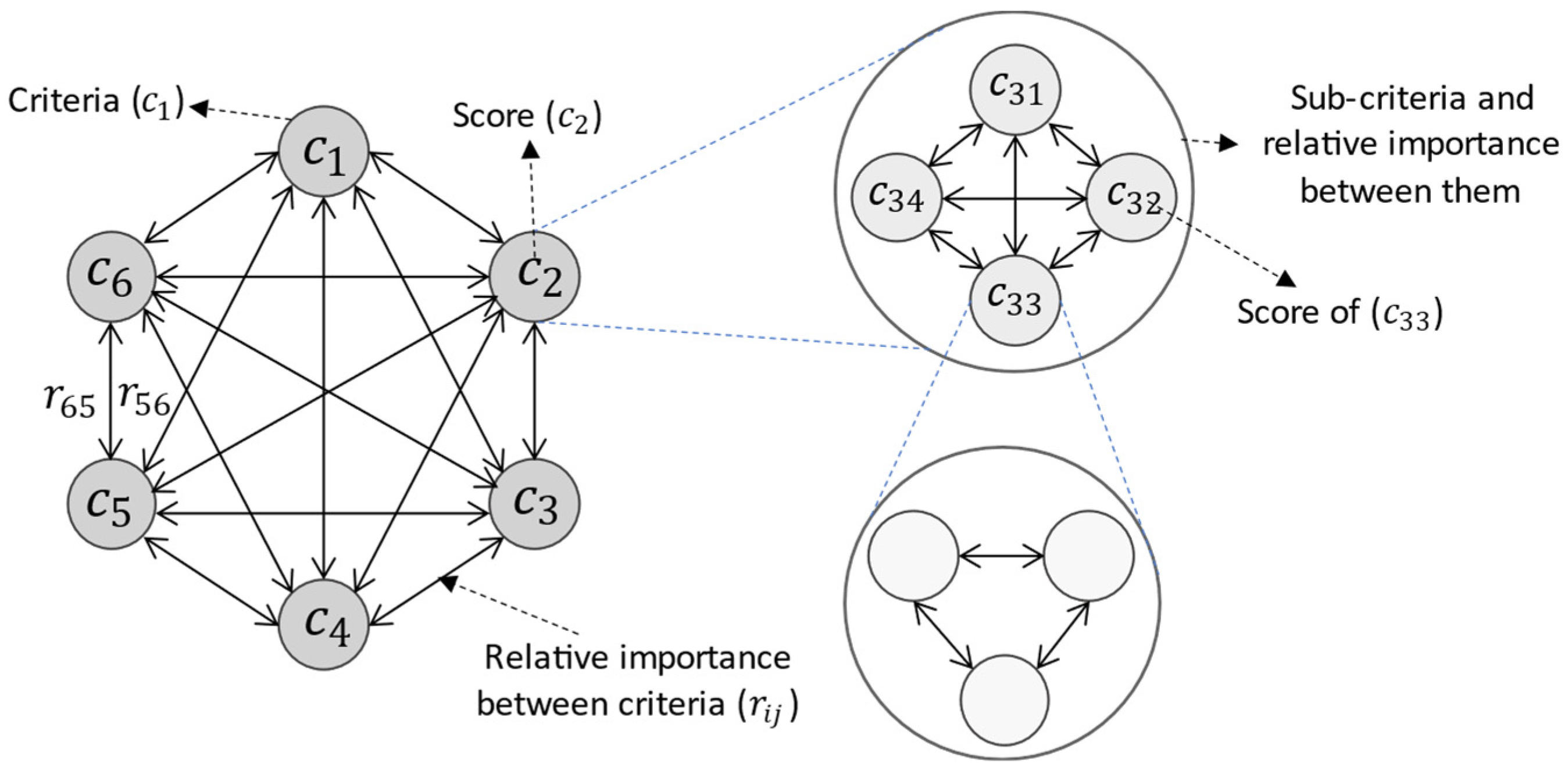
Step 1 (identification of criteria, sub-criteria, and alternatives of the problem): Identification of the affecting factor on the process using the available data in the literature or conducting a survey of experts [48] is presented by representing graph and their dependencies. The reliability affecting factors have been described before. In the representation of the graph, as shown in Figure 3, there is a set of nodes and a set of directed edges. Each node ${𝓃}_i$ is the identifier of the $i$-th criterion for alternative selection and the edges represent the relative importance of criteria, in which the number of nodes and alternatives are identical. In alternative selection, if node $i$ is more important than node $𝒿$, a directed edge is drawn from $i$ to $𝒿$ (${ℯ}_{i𝒿}$) and vice versa [46]. An example of the decision-making structure by the use of the permanent matrix is given in Figure 3.

Step 2 (definition of the relative importance of criteria and alternatives score): In this step, if the criterion is qualitative, the values of the alternatives score can be calculated by rating a scale from zero to one [30], as shown in

Table 2. Quantitative scores of alternatives.

Qualitative Measure	Crisp Score	Qualitative Measure	Crisp Score
Exceptionally Low	0	Above average	6
Extremely Low	1	High	7
Very Low	2	Very high	8
Low	3	Extremely high	9
Below average	4	Exceptionally high	10
Average	5

.

If the criterion is quantitative, it should be normalised. Therefore, if ${𝓋}_i$ is the criteria value of alternative $i$ and ${𝓋}_{𝒿}$ is the criteria value of alternative $𝒿$, $\frac{{𝓋}_i}{{𝓋}_{𝒿}}$ should be normalised [47]. After calculating all the criteria values for each alternative, we define the ratio criteria matrix for them.

$$\left[\psi \right]=\left[\begin{array}{cccc}{𝒞}_{11}& 0& \dots & 0\\ 0& {𝒞}_{22}& \dots & 0\\ \dots & \dots & \dots & \dots \\ 0& 0& \dots & {𝒞}_{𝓃𝓃}\end{array}\right]$$

(10)

On the other hand, the relative importance between criteria (${𝓇}_{i𝒿}$) can get the values between zero and one. The relationship between ${𝓇}_{i𝒿}$ and ${𝓇}_{𝒿i}$ is not necessarily a compensatory relationship. It can be ${𝓇}_{𝒿i}=\frac{1}{{𝓇}_{i𝒿}}$ as shown in

Table 3. The relative importance of criteria.

Class Definition	${\mathit{𝓇}}_{\mathit{𝒾}\mathit{𝒿}}$	${\mathit{𝓇}}_{\mathit{𝒿}\mathit{𝒾}} = 1 - {\mathit{𝓇}}_{\mathit{𝒾}\mathit{𝒿}}$
Two criteria equally important	0.5	0.5
One criterion is slightly more important than others	0.6	0.4
One criterion more important than others	0.7	0.3
One criterion very important than others	0.8	0.2
One criterion exceptionally important than others	0.9	0.1
One criterion most important, other not important	1.0	0.0

.

The relative importance matrix is defined at the end of this step as:

$$\left[\beta \right]=\left[\begin{array}{cccc}0& {𝓇}_{12}& \dots & {𝓇}_{i𝓃}\\ {𝓇}_{21}& 0& \dots & {𝓇}_{2𝓃}\\ \dots & \dots & \dots & \dots \\ {𝓇}_{𝓃1}& \dots & \dots & 0\end{array}\right]$$

(11)

Step 3 (calculation of the alternative evaluation matrix): In this step, after identifying $\beta$ and $\psi$, the alternative evaluation matrix $\mathsf{\xi }$ is calculated by:

$$\zeta =\psi +\beta =\left[\begin{array}{ccccc}{𝒞}_1& {𝓇}_{12}& {𝓇}_{13}& \dots & {𝓇}_{1𝓃}\\ {𝓇}_{21}& {𝒞}_2& {𝓇}_{23}& \dots & {𝓇}_{2𝓃}\\ {𝓇}_{31}& {𝓇}_{32}& {𝒞}_3& \dots & {𝓇}_{3𝓃}\\ \dots & \dots & \dots & \dots & \dots \\ {𝓇}_{𝓃1}& {𝓇}_{𝓃2}& {𝓇}_{𝓃3}& \dots & {𝒞}_{i𝓃}\end{array}\right]$$

(12)

The permanent of this matrix is the criteria function of alternative selection [30]. This value gives a grade for the alternatives that must be dissentingly sorted, and the alternative with the largest permanent value will be the best alternative (the most reliable route) [49]. The following equation represents the function for calculating the permanent value.

$$\begin{array}{ll}\mathrm{per}\left(\mathsf{\xi }\right)& ={\displaystyle {\displaystyle \prod }_{i=1}^{\mathcal{N}}}{\mathrm{c}}_{\mathrm{i}}+{\displaystyle {\displaystyle \sum }_{i,𝒿\dots \mathcal{N}}}({𝓇}_{i𝒿}.{𝓇}_{𝒿i}).c_{𝓀}.c_{𝓁}\dots c_{\mathcal{N}}+{\displaystyle {\displaystyle \sum }_{i,𝒿\dots \mathcal{N}}}({𝓇}_{i𝒿}.{𝓇}_{𝒿𝓀}.{𝓇}_{𝓀i}\\ & \hspace{1em}\hspace{1em}\hspace{1em}\hspace{1em}+{𝓇}_{i𝓀}.{𝓇}_{𝓀𝒿}.{𝓇}_{𝒿i}).c_{𝓁}.c_{𝓃}\dots c_{\mathcal{N}}\\ & \hspace{1em}\hspace{1em}\hspace{1em}\hspace{1em}+\left\{\{{\displaystyle {\displaystyle \sum }_{\mathrm{i},\mathrm{j}\dots \mathrm{N}}}({𝓇}_{i𝒿}.{𝓇}_{𝒿i})\left({𝓇}_{𝓀𝓁}.{𝓇}_{𝓁𝓀}\right).c_{𝓃}.c_{𝓂}\dots .c_{\mathcal{N}}+{\displaystyle {\displaystyle \sum }_{i,𝒿\dots \mathcal{N}}}({𝓇}_{i𝒿}.{𝓇}_{𝒿𝓀}.{𝓇}_{𝓀𝓁}.{𝓇}_{𝓁i}\hspace{1em}+{𝓇}_{i𝓁}.{𝓇}_{𝓁𝓀}.{𝓇}_{𝓃𝒿}.{𝓇}_{𝒿i}).c_{𝓃}.c_{𝓂}\dots .c_{\mathcal{N}}\right\}\\ & \hspace{1em}\hspace{1em}\hspace{1em}\hspace{1em}+[{\displaystyle {\displaystyle \sum }_{i,𝒿\dots \mathcal{N}}}({𝓇}_{i𝒿}.{𝓇}_{𝒿i})\left({𝓇}_{𝓀𝓁}.{𝓇}_{𝓁𝓃}.{𝓇}_{𝓃𝓀}\right).{\mathrm{c}}_{𝓂}.{\mathrm{c}}_{ℴ}\dots {\mathrm{c}}_{\mathcal{N}}\\ & \hspace{1em}\hspace{1em}\hspace{1em}\hspace{1em}+{\displaystyle {\displaystyle \sum }_{i,𝒿\dots \mathcal{N}}}({𝓇}_{i𝒿}.{𝓇}_{𝒿𝓀}.{𝓇}_{𝓀𝓁}.{𝓇}_{𝓁𝓃}.{𝓇}_{𝓃i}+{𝓇}_{i𝓃}.{𝓇}_{𝓃𝓁}.{𝓇}_{𝓁𝓀}.{𝓇}_{𝓀𝒿}.{𝓇}_{𝒿i}).{\mathrm{c}}_{𝓂}.{\mathrm{c}}_{ℴ}\dots {\mathrm{c}}_{\mathcal{N}}]\\ & \hspace{1em}\hspace{1em}\hspace{1em}\hspace{1em}+\dots \end{array}$$

(13)

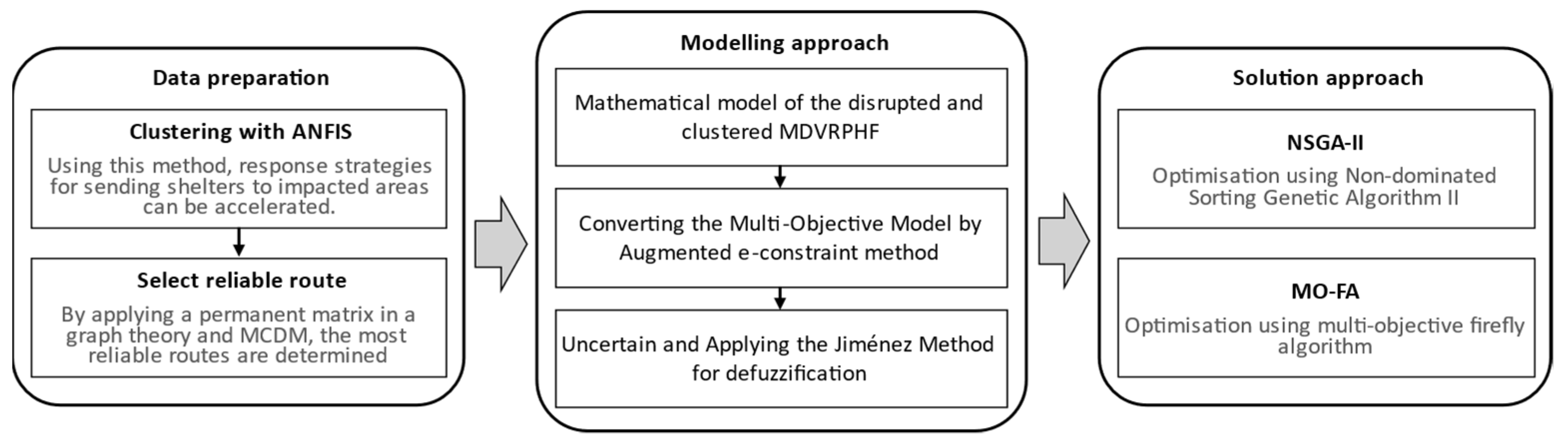
3.3. Modelling and the Proposed Solving Method

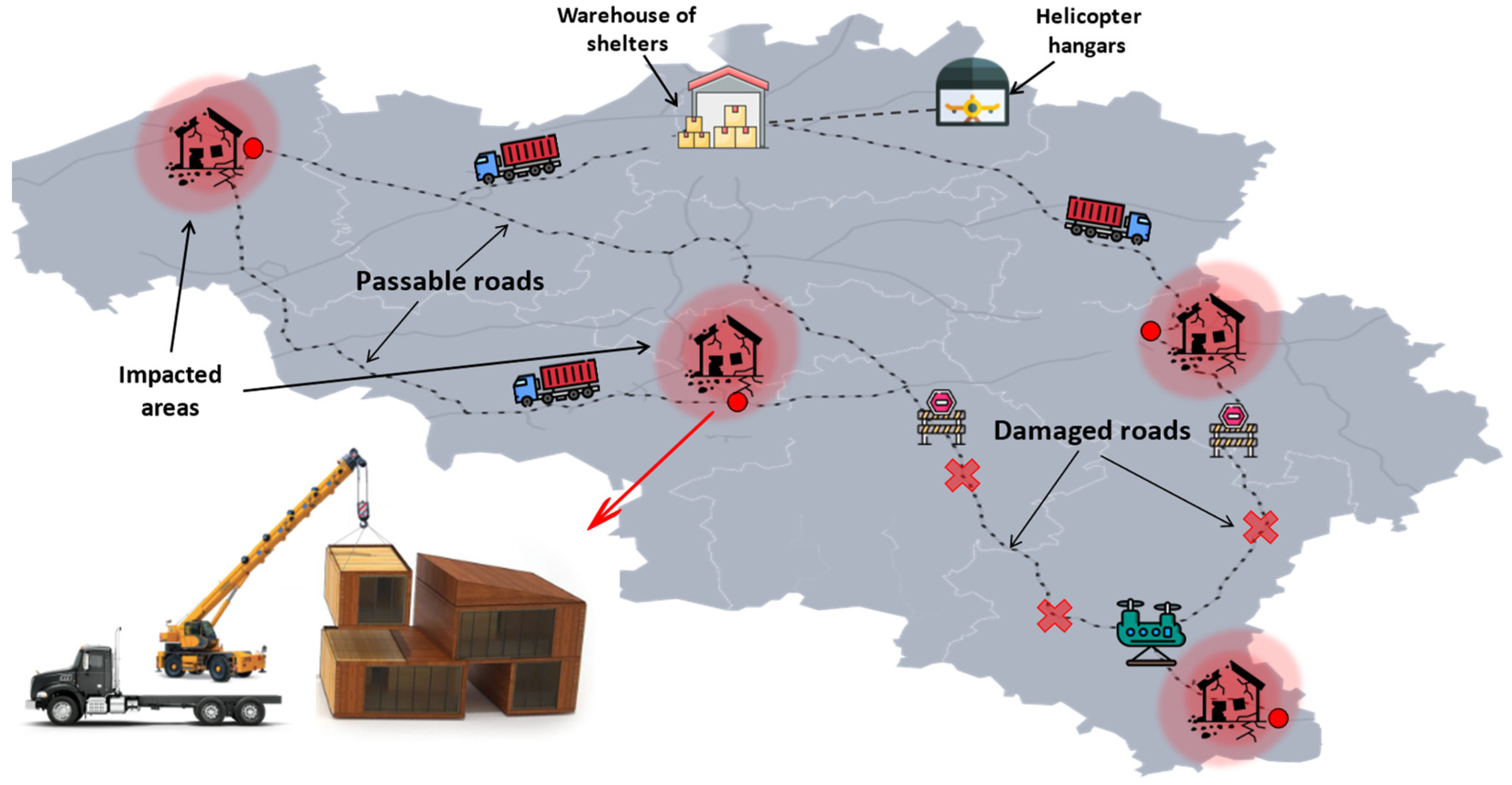
Consider a disaster-affected area. Humanitarian organisations have a plan to send temporary shelters to the affected areas using trucks and helicopters in response to this disaster. Multiple depots are considered in response operations, including the depot of heterogeneous trucks and the hangers of heterogeneous helicopters. It should be noted that the vehicle depot also serves as a shelter warehouse. These vehicles should deliver temporary shelters to demand points. However, due to the severity of the disaster, some infrastructures, including access roads to some of these points, have been disrupted, making ground delivery to these points impossible. As a result, the affected areas have been divided into two clusters in order to reduce the time it takes to send shelters. Because of the disruptions in the access roads, the affected points in one cluster can receive shelters in both ground and air modes, while the points in the other cluster can only receive shelters in an air mode due to the breakdown of their road. The points in each cluster are then prioritised separately by the key factors on route reliability. That is, in each cluster, the shelters are distributed first to the most reliable route, and the vehicles serve from the most reliable routes. On the other hand, during the distribution of shelters, the ground vehicle (e.g., truck) breaks down, causing its service areas to be served late and causing disruption in the distribution system (Figure 4 shows a schematic sample of the problem).

Mathematical modelling approaches can effectively condense and highlight the most important aspects of our understanding of real-world decision-making problems. These problems, however, are frequently complex. Real-world problems can be too complex or challenging to model if all details are taken into account, so it is important to keep this in mind when developing models. Therefore, effective models rely heavily on assumptions that reduce complexity while retaining the system’s fundamental properties. Because of this, it is crucial to simplify assumptions in order to keep models tractable and true to the underlying system. These assumptions lead to a highly effective mathematical model, as shown by the following:

• There is a limitation in the number of vehicles, and various types are used to transport shelters to affected areas.
• All vehicles’ starting points are known and defined, as is which vehicle belongs to which depot.
• All vehicles should be utilised in the event of a large-scale disaster.
• Each affected point is served by a single-vehicle.
• The depot inventory is sufficient to respond to the affected areas.
• The location of any affected area is known, as is its distance from depots.
• The amount of demand is known at each affected point.
• Each vehicle returns to its starting place at the end of the operation.
• The affected points are divided into two clusters, and all impacted areas in each cluster are prioritised based on reliability-affecting factors.
• The broken-down vehicle cannot be repaired in a reasonable amount of time so that it can be used again.
• The problem is scenario-based, and the vehicle’s failure time is known under various scenarios.
• If the product is delivered to the affected point, the service is completed, and the shortage is avoided. After the vehicle fails, the other vehicle should not perform its serving duties and must follow their specified plan.
• The affected areas’ demand is fuzzy, with a triangular fuzzy number.
• Each affected area’s demand can be partially met, and a shortage is acceptable.

3.3.1. Mathematical Model of the Disrupted and Clustered MDVRPHF

The mathematical model is developed using the variables and parameters listed below.

Notations and sets

${𝓋}^{\prime }$	Set of land vehicles
${𝓋}^{″}$	Set of aerial vehicles
$ℯ$	Set of the impacted areas with a passable road
${ℯ}^{\prime }$	Set of the impacted areas with a damaged road
$𝒹$	Set of the ground vehicle depots
${𝒹}^{\prime }$	Set of the helicopter hangars
$\mathcal{V}$	Set of vehicles
$\mathcal{S}$	Set of scenarios
$\mathcal{N}$	Number of all nodes
${𝓃}_{{𝓋}^{\prime } }$	Number of trucks
${𝓃}_{{𝓋}^{″}}$	Number of helicopters
${𝓃}_{ℯ}$	Number of impacted areas with a passable road
${𝓃}_{{ℯ}^{\prime }}$	Number of impacted areas with a damaged road
${𝓃}_{𝒹}$	Number of truck depots
${𝓃}_{{𝒹}^{\prime }}$	Number of helicopter hangars

Parameters

${\mathsf{\chi }}_{𝓋}$	The capacity of vehicle v
$\widetilde{{\mathrm{Dem}}_i}$	The demand of shelters for node $i$ (impacted area)
${𝓉}_{𝓋i𝒿}$	Travel time from node $i$ to $𝒿$ for vehicle $𝓋$
${𝓇}_{i𝒿}$	The permanent value of node $i$ to $𝒿$ based on the reliability index
${𝒰}_{𝓋i}$	The auxiliary and sequential variable that shows the number of nodes being visited with vehicle $𝓋$ in sub-tour elimination constraints
${𝒯}_{i𝓋}$	Arrival time of vehicle $𝓋$ to node $i$
${\mathsf{\theta }}_{i𝒿}$	Travel time of a vehicle from node $i$ to node $𝒿$

Decision Variable

$$x_{𝓋i𝒿}=\{\begin{array}{cc}1& \mathrm{if} \mathrm{vehicle} 𝓋 \mathrm{travel} \mathrm{from} \mathrm{node} i \mathrm{to} \mathrm{node} 𝒿\\ 0& \mathrm{otherwise}\end{array}$$

$${𝓎}_i^{𝓈}=\{\begin{array}{cc}1& \mathrm{if} \mathrm{the} \mathrm{shelter} \mathrm{is} \mathrm{not} \mathrm{delivered} \mathrm{to} \mathrm{impacted} \mathrm{area} 𝒿 \mathrm{under} \mathrm{scenario} 𝓈\\ 0& \mathrm{otherwise}\end{array}$$

Model Formulation

The following is a mathematical formulation of the suggested model:

$$\mathrm{Min} (\mathrm{Max}{\displaystyle \sum }_{i\in ℐ}{\displaystyle \sum }_{𝒿\in 𝒥}{\displaystyle \sum }_{𝓋\in 𝒱}{𝓉}_{𝓋i𝒿}{x}_{𝓋i𝒿})$$

(14)

$$\mathrm{Min} ({\displaystyle \sum }_{i\in ℐ}{\displaystyle \sum }_{𝒿\in 𝒥}{\displaystyle \sum }_{𝓋\in 𝒱}{𝓇}_{i𝒿}{x}_{𝓋i𝒿})$$

(15)

$$\mathrm{Min} {\displaystyle \sum }_{\mathrm{s}}{\displaystyle \sum }_{i\in {𝓃}_{ℯ}\cup {𝓃}_{{ℯ}^{\prime }}}{𝓎}_i^{\mathrm{s}} \times \widetilde{{\mathrm{dem}}_i}$$

(16)

$$\mathrm{s}.\mathrm{to}.$$

$${\displaystyle \sum }_{i\in {𝓃}_{ℯ}\cup 𝒻\left(𝓋,i\right)}{x}_{𝓋𝒿i} = {\displaystyle \sum }_{i\in {𝓃}_{ℯ}\cup 𝒻\left(𝓋,i\right)}{x}_{𝓋𝒿i},\forall 𝒿\in {𝓃}_{ℯ},v\in {𝓃}_{{𝓋}^{\prime }}$$

(17)

$${\displaystyle \sum }_{i\in {𝓃}_{ℯ}\hspace{0.33em}\cup {𝓃}_{{ℯ}^{\prime }}\cup 𝒻\left(𝓋,i\right)}{x}_{𝓋i𝒿} = {\displaystyle \sum }_{i\in {𝓃}_{ℯ}\hspace{0.33em}\cup {𝓃}_{{ℯ}^{\prime }}\cup 𝒻\left(𝓋,i\right)}{x}_{𝓋𝒿i},\forall \hspace{0.33em}𝒿\in {𝓃}_{ℯ}\cup {𝓃}_{{ℯ}^{\prime }},v\in {𝓃}_{{𝒹}^{\prime }}$$

(18)

$${\displaystyle \sum }_{\begin{array}{c}i\in f\left(v,i\right)\\ \hspace{0.33em}\\ \end{array}}{\displaystyle \sum }_{𝒿\in {𝓃}_{ℯ}}{x}_{𝓋i𝒿}=1,\forall \hspace{0.33em}\mathrm{v}\in {𝓃}_{{𝓋}^{\prime }},\forall 𝒻\left(𝓋,i\right)$$

(19)

$${\displaystyle \sum }_{\begin{array}{c}i\in f\left(v,i\right)\\ \hspace{0.33em}\hspace{0.33em}\\ \end{array}}{\displaystyle \sum }_{𝒿\in {𝓃}_{ℯ}\cup {𝓃}_{{ℯ}^{\prime }}}{x}_{𝓋i𝒿}=1,\forall \hspace{0.33em}\mathrm{v}\in {𝓃}_{{𝒹}^{\prime }}$$

(20)

$${\displaystyle \sum }_{\begin{array}{c}i\in {𝓃}_{ℯ}\\ \hspace{0.33em}\hspace{0.33em}\\ \end{array}}{\displaystyle \sum }_{𝒿\in 𝒻\left(𝓋,i\right)}{x}_{𝓋i𝒿}=1,\forall \hspace{0.33em}\mathrm{v}\in {𝓃}_{{𝓋}^{\prime }}$$

(21)

$${\displaystyle \sum }_{i\in {𝓃}_{ℯ}\cup {𝓃}_{{ℯ}^{\prime }}}{\displaystyle \sum }_{𝒿\in 𝒻\left(𝓋,i\right)}{x}_{𝓋i𝒿}=1,\forall \mathrm{v}\in {𝓃}_{{𝒹}^{\prime }}$$

(22)

$${\displaystyle \sum }_{𝓋\in {𝓃}_{{𝓋}^{\prime } }}{\displaystyle \sum }_{𝒿\in {𝓃}_{ℯ}}{x}_{𝓋i𝒿}+{\displaystyle \sum }_{\mathrm{v}\in {𝓃}_{{𝓋}^{″} }}{\displaystyle \sum }_{𝒿\in {𝓃}_{ℯ}\cup {𝓃}_{{ℯ}^{\prime }}\cup 𝒻\left(𝓋,i\right)}{x}_{𝓋i𝒿}=1,\forall i\in {𝓃}_{ℯ}$$

(23)

$${\displaystyle \sum }_{𝓋\in {𝓃}_{{𝓋}^{″} }}{\displaystyle \sum }_{𝒿\in {𝓃}_{ℯ}\cup {𝓃}_{{ℯ}^{\prime }}\cup 𝒻\left(𝓋,i\right)}{x}_{𝓋i𝒿}=1,\forall i\in {𝓃}_{{ℯ}^{\prime }}$$

(24)

$${\displaystyle \sum }_{𝒿\in {𝓃}_{ℯ}\cup 𝒻\left(𝓋,i\right)}{\displaystyle \sum }_{i\in {𝓃}_{ℯ}}{x}_{𝓋i𝒿}\times \widetilde{{\mathrm{dem}}_i}\le {\mathsf{\chi }}_{𝓋},\forall \hspace{0.33em}𝓋\in {𝓃}_{𝒹}\cup {𝓃}_{{𝒹}^{\prime }}$$

(25)

$${\displaystyle \sum }_{𝒿\in {𝓃}_{ℯ}\cup {𝓃}_{{ℯ}^{\prime }}}{\displaystyle \sum }_{i\in {𝓃}_{ℯ}\cup {𝓃}_{{ℯ}^{\prime }}}{x}_{𝓋i𝒿}\times \widetilde{{\mathrm{dem}}_i}\le {\mathsf{\chi }}_{𝓋},\forall \hspace{0.33em}𝓋\in {𝓃}_{{𝓋}^{″}}$$

(26)

$${\mathcal{U}}_{𝓋i}-{\mathcal{U}}_{𝓋𝒿}+{𝓃}_{ℯ}{x}_{𝓋i𝒿}\le \hspace{0.33em}{𝓃}_{ℯ}-1,\forall \hspace{0.33em}𝓋\in {𝓃}_{{𝓋}^{\prime }},\forall i\in 𝓃,\forall i\in {𝓃}_{ℯ}$$

(27)

$${\mathcal{U}}_{𝓋i}-{\mathcal{U}}_{𝓋𝒿}+{𝓃}_{{ℯ}^{\prime }}{x}_{𝓋i𝒿}\le \hspace{0.33em}{𝓃}_{{ℯ}^{\prime }}-1,\forall 𝓋\in {𝓃}_{{𝓋}^{″}},\forall i\in {𝓃}_{ℯ}\cup {𝓃}_{{ℯ}^{\prime }},\forall i\in {𝓃}_{ℯ}\cup {𝓃}_{{ℯ}^{\prime }}$$

(28)

$${\mathcal{U}}_{𝓋i}\le {𝓃}_{ℯ},\forall 𝓋\in {𝓃}_{{𝓋}^{\prime }},\forall i\in {𝓃}_{ℯ}$$

(29)

$${\mathcal{U}}_{𝓋.𝒻\left(𝓋,i\right)}=0,\forall 𝓋\in {𝓃}_{{𝓋}^{\prime } },\forall i\in {𝓃}_{ℯ}$$

(30)

$${\mathcal{U}}_{𝓋i}\le {𝓃}_{ℯ}\cup {𝓃}_{{ℯ}^{\prime }},\forall 𝓋\in {𝓃}_{{𝓋}^{″}},\forall i\in {𝓃}_{ℯ}\cup {𝓃}_{{ℯ}^{\prime }}$$

(31)

$${\mathcal{U}}_{𝓋.𝒻\left(𝓋,i\right)}=0,\forall 𝓋\in {𝓃}_{{𝓋}^{″}},\forall i\in {𝓃}_{ℯ}\cup {𝓃}_{{ℯ}^{\prime }}$$

(32)

$${\displaystyle \sum }_{𝓋}{\mathcal{T}}_{i𝓋}=0,\forall 𝒻\left(𝓋,i\right)$$

(33)

$${\mathcal{T}}_{𝒿𝓋}={\displaystyle \sum }_{𝒿\in {𝓃}_{ℯ}\cup {𝓃}_{{ℯ}^{\prime }}}{x}_{𝓋i𝒿}\times \left({\mathcal{T}}_{i𝓋}+{\mathsf{\theta }}_{i𝒿}\right),\forall \hspace{0.33em}i\in {𝓃}_{ℯ}\cup {𝓃}_{{ℯ}^{\prime }}$$

(34)

$$\mathrm{bigM}\left(1-{𝓎}_i^{𝓈}\right)\ge \left({\mathcal{T}}_{i𝓋}-{\phi }_{𝓋}^{𝓈}\right),\forall \hspace{0.33em}i\in {𝓃}_{ℯ}\cup {𝓃}_{{ℯ}^{\prime }},𝓈\in \mathcal{S},𝓋\in {𝓃}_{𝓋}$$

(35)

$${\mathcal{U}}_{𝓋i}=\left\{0,1,2,\dots .\right\}$$

(36)

$$x_{𝓋i𝒿}\in \left\{0,1\right\},\forall 𝓋,i,𝒿$$

(37)

$${\mathcal{T}}_{i𝓋}\ge 0$$

(38)

$${\mathsf{\phi }}_{𝓋}^{𝓈} \ge 0$$

(39)

$${\mathsf{\theta }}_{i𝒿}\ge 0$$

(40)

$${𝓎}_i^{𝓈}\in \left\{0,1\right\}$$

(41)

The objective function (14) minimises the maximum of the transportation time of vehicle v between nodes i and j. The objective function (15) maximises the reliability of routes by maximising the sum of the permanent of each route. The objective function (16) minimises the unmet demand at impacted area i under scenario s. Constraint (17) guarantees the flow balance for the impacted areas with reliable road and ground vehicles. That is, each truck, after entering the node and servicing the area, leaves the node. Constraint (18) guarantees the balance of flow for healthy and not-healthy areas and for helicopters. In other words, the helicopters leave the node after its entrance. Constraint (19) indicates that the start point of any truck is known to be from what depot, while constraint (20) is the constraint on the start point of helicopters. Constraints (21) and (22) guarantees that any vehicles (i.e., truck and helicopter) after servicing any nodes must come back to the start point and the route is closed. Constraint (23) ensures that each vehicle (i.e., helicopter or truck) only serve one node (for points that their leading road is healthy). Consequently, constraint (24) identifies that each vehicle (i.e., helicopter) serve only one not healthy node (the impacted area that its leading road is damaged). Constraints (25) and (26) are the capacity limitation of trucks and helicopters. The part considered as a sub-tour constraint is represented in Constraints (27) to (32), in which Constraints (27) and (28) are the sub-tour elimination constraints for trucks and helicopters. Following that, Constraints (29) and (30) are the sub-tour elimination constraints for axillary variables ${\mathcal{U}}_{i𝒿}$ and ${\mathcal{U}}_{𝓋𝒻\left(𝓋,i\right)}$ for trucks. Constraints (31) and (32) are the sub-tour elimination constraints for axillary variables ${\mathcal{U}}_{𝓋i }$ and ${\mathcal{U}}_{𝓋𝒻\left(𝓋,i\right)}$ for helicopters. Constraint (33) ensures that all vehicles depart from the depots. Constraint (34) calculates the reaching time of the vehicle to the demand centre or impacted areas. Constraint (35) identifies whether the shortage is present under the given scenarios or not. In other words, whether the shelters delivered to impacted areas under the different scenarios or not (if the product has been delivered to the impacted area means that the vehicle has not been failed before serving the impacted area and the shortage has not incurred). If ${\mathrm{T}}_{i𝓋}-{\phi }_{𝓋}^{𝓈}>0$ means that the failure time of vehicle is after the failure time at scenario s. Consequently, the shortage will occur, and the vehicle is not arrived to the impacted area. Otherwise, the vehicle has break downed after serving and all the goods are delivered to the affected areas and are not faced with shortage (to identify the shortage, we calculate the time of serving each point). Constraints (36) and (37) refer to the sequential ${𝓊}_{i𝓋}$ and binary variables $x_{𝓋i𝒿}$, respectively. Constraint (38) implies to the arriving time of vehicle v to node i, which is a non-negative value. Constraint (39) implies the failure time of vehicle v under scenario s that is a non-negative. Constraint (40) identifies the vehicle travel time and transfers from node i to node j, a non-negative value. Constraint (41) is a binary variable that identifies the presence or absence of shortage.

3.3.2. Converting the Multi-Objective Model to a Single Objective Model by the Augmented ε-Constraint Method

Among the available techniques in the transformation of the multi-objective problem to a single objective problem, the augmented ε-constraint method is applied. This method is one of the efficient methods in looking for Pareto optimised solutions, in which the first objective function is optimised, and other objectives are being added to the constraints [50]. In the general, the other name of the ε-constraint method is a trade-off or ε-constraint method [51]. Consider a multi-objective programming, where p is the number objectives, ${\mathrm{f}}_i\left(x\right) i=1,2,\dots ,𝓅$ and $x\in 𝒮$ is the decision variable, which S is the feasible space. Now, we suppose that all objective functions are maximisation without a loss of generality. When we apply the ε-constraint method, we must consider one of the objective functions as the main objective and add others to the constraints. Following is the structure of Formula (41) [52].

$$\max {𝒻}_1\left(x\right)$$

(42)

$$\mathrm{s}.\mathrm{to}.$$

(43)

$${𝒻}_2\left(x\right)\le {\mathsf{\epsilon }}_2$$

(44)

$${𝒻}_3\left(x\right)\le {\mathsf{\epsilon }}_3$$

$$..$$

$${𝒻}_{𝓅}\left(x\right)\le {\mathsf{\epsilon }}_{𝓅}$$

(45)

$$x\in 𝒮$$

(46)

The other objective functions with permissible values ${\mathsf{\epsilon }}_{\mathrm{i}}$, are constrained (so that $i ϵ 1,2,\dots ,𝓂 \backslash 𝓃,$ $𝓃$ is the index of the main objective function) [51]. The Pareto-optimal values are obtained by adding the right-hand side of new constraints (ε vector) [53]. When this method is used, the region of at least p-1 objective function, for the definition of grid points, must be defined for each ${\mathsf{\epsilon }}_i$. An efficient method for identification of this region is to apply a payoff table for each objective function, which the difference between the minimum value (${𝒻}_i^{\min }$) and the maximum value (${𝒻}_i^{\max }$) constitute the region.

$${𝓇}_i={𝒻}_i^{max}-{𝒻}_i^{min}$$

(47)

Then, this region for each objective function is divided into equal intervals and according to the following formula: the set of ${𝓆}_i+1$ grid points is calculated.

$${\mathsf{\epsilon }}_i^{𝓀}={𝒻}_i^{max}-\frac{{𝓇}_i}{{𝓆}_i}\ast 𝓀,𝓀=0,1,\dots ,{𝓆}_i$$

(48)

${{\displaystyle \prod }}_{i=2}^{𝓅}({𝓆}_i+1)$ single optimisation sub-problem must be produced from the multi-objective problem, which any sub-problem has a Pareto-optimal solution. Because of adding objective functions, the constraints may be infeasible. One drawback of this method is that it may produce inefficient solutions [52]. Different versions of the ε-constraint method are developed for producing more efficient solutions. To overcome this drawback, an augmented ε-constraint method is proposed, in which changing the constraints of the objective functions, by using of slack or surplus variables, is suggested, and the main objective function is augmented by the sum of slack or surplus values. We have the following model [53]:

$$\mathrm{Max} \left\{{𝒻}_1\left(x\right)+\mathsf{\delta }\ast \left({𝓈}_2+{𝓈}_3+\dots +{𝓈}_{𝓅}\right)\}\right.$$

$$\mathrm{S}.\mathrm{t}.$$

(49)

$${𝒻}_2\left(x\right)={\mathsf{\epsilon }}_2-{𝓈}_2$$

(50)

$${𝒻}_3\left(x\right)={\mathsf{\epsilon }}_3-{𝓈}_3$$

(51)

$$..$$

$${𝒻}_{𝓅}\left(x\right)={\mathsf{\epsilon }}_{𝓅}-{𝓈}_{𝓅}$$

(52)

$$x\in \mathrm{X},{𝓈}_i\in {\mathrm{R}}^{+}$$

(53)

where the δ value is a small number between 10⁻⁶ and 10⁻³.

3.3.3. Uncertainty and Defuzzification

In the proposed model, due to the uncertainty in an emergency situation and becoming closer to reality, the demand of the impacted areas is fuzzy numbers (parameter $De{m}_i$ is considered a triangle fuzzy number). Because of the applicability and simplicity in calculations, a symmetrical triangle distribution is considered for specifying of the fuzzy parameter [54,55]. To transform a linear mathematical model to its corresponding deterministic model, the Jimenez method is applied because of the high efficiency [56]. The membership function of the fuzzy parameter is as follows [57]:

$${\mu }_{\tilde{c}}\left(x\right)=\left\{\begin{array}{ll}{f}_c\left(x\right)=\frac{x-c^p}{c^{𝓂}-c^p}\hfill & if c^p\le x\le c^{𝓂}\hfill \\ 1\hfill & if x=c^{𝓂}\hfill \\ g_c\left(x\right)=\frac{c^0-x}{c^0-c^{𝓂}}\hfill & if c^{𝓂}\le x\le c^0\hfill \\ 0\hfill & if x\le c^p or x\ge c^0\hfill \end{array}\right.$$

(54)

Also, for fuzzy number $\widetilde{𝒶}$ and ${𝑏}^{˜}$ the degree of being greater is defined by:

$${\mu }_{\mathcal{M}}\left(\widetilde{𝒶},\widetilde{𝒷}\right)=\left\{\begin{array}{ll}0\hfill & if E_2^0 - E_1^{𝒷}\prec 0\hfill \\ \frac{E_2^{𝒶}-E_1^{𝒷}}{E_2^{𝒶}-E_1^{𝒷}-\left(E_1^{𝒶}-E_2^{𝒷}\right)}\hfill & if E_1^{𝒶}-E_2^{𝒷}\prec 0\prec E_2^{𝒶}-E_1^{𝒷}\hfill \\ 1\hfill & if E_1^0-E_2^{𝒷}\succ 0\hfill \end{array}\right.$$

(55)

${\mu }_{\mathcal{M}}\left(\widetilde{𝒶},\widetilde{𝒷}\right)$ Identifies the degree that $\widetilde{𝒶}$ is greater than $\widetilde{𝒷}$. When ${\mu }_{\mathcal{M}}\left(\widetilde{𝒶},\widetilde{𝒷}\right)\ge \mathsf{\alpha }$, it is said that $\widetilde{𝒶}$ is greater than $\widetilde{𝒷}$ at least by degree α” [56]. Consider the mathematical model with fuzzy parameters as follows:

$$\mathrm{Min}Z=C^{˜}t𝑥$$

(56)

$$\mathrm{S}.\mathrm{t}.$$

$$𝑋\in {𝐴}^{˜}=\{𝑥\in Rn|\tilde{a}i𝑥\ge b^{˜}i,i = 1,\dots ,m, 𝑥 \ge 0$$

(57)

where $\widetilde{𝒷}$ = (${\widetilde{𝒷}}_1$, ${\widetilde{𝒷}}_2$, …, ${\widetilde{𝒷}}_{𝓃}$), $\tilde{c}$ = (${\tilde{c}}_1$, ${\tilde{c}}_2$, …, ${\tilde{c}}_{𝓃}$) and $\tilde{\mathcal{A}}$ = ${\left[{\widetilde{𝒶}}_{i𝒿}\right]}_{𝓂 \times 𝓃 }$ are the objective functions and constraints’ parameters [58]. Applying the Jimenez method, the above model is transformed to the deterministic parametric linear programming method.

$$\begin{gathered} minz = {\tilde{c}}_{𝓉}x \\ s.t. \\ {\widetilde{𝒶}}_{i}x\ge {\widetilde{𝒷}}_i \\ {\widetilde{𝒶}}_{𝒿}x={\widetilde{𝒷}}_i \\ x\ge 0 \end{gathered}$$

$$\begin{gathered} \mathrm{Equivalent} \mathrm{crisp}-\mathrm{parametric} \mathrm{model} \alpha \\ \to \end{gathered}$$

$$\begin{gathered} \min \mathrm{z}=\mathrm{EV}\left(\tilde{c}\right)x \\ \mathrm{s}.\mathrm{t} \\ \left[\left(1-\mathsf{\alpha }\right){\mathrm{E}}_2^{{𝒶}_{𝒿}}+{\mathsf{\alpha }\mathrm{E}}_1^{{𝒶}_i}\right]x\ge {\mathsf{\alpha }\mathrm{E}}_2^{{𝒷}_{𝒿}}+\left(1-\mathsf{\alpha }\right){\mathrm{E}}_1^{{𝒷}_{𝒿}} \\ \left[\left(1-\frac{\mathsf{\alpha }}{2}\right){\mathrm{E}}_2^{{𝒶}_{𝒿}}+{\mathsf{\alpha }\mathrm{E}}_1^{{𝒶}_{𝒿}}\right]x\ge \frac{\mathsf{\alpha }}{2}{\mathrm{E}}_2^{{𝒷}_{𝒿}}+\left(1-\frac{\mathsf{\alpha }}{2}\right){\mathrm{E}}_1^{{𝒷}_{𝒿}} \\ \left[\left(\frac{\mathsf{\alpha }}{2}\right){\mathrm{E}}_2^{{𝒶}_{𝒿}}+\left(1-\frac{\mathsf{\alpha }}{2}\right){\mathrm{E}}_1^{{𝒶}_{𝒿}}\right]x\ge \left(1-\frac{\mathsf{\alpha }}{2}\right){\mathrm{E}}_2^{{𝒷}_{𝒿}}+\frac{\mathsf{\alpha }}{2}{\mathrm{E}}_1^{{𝒷}_{𝒿}} \\ x\ge 0 \end{gathered}$$ (58)

where α is the possibility level of non-deterministic data and expected interval (EI($\tilde{c}$)) and expected value (EV($\tilde{c}$)) are defined by [28].

$$EI\left(\overline{c}\right) = \left[E_1^c.E_c^2\right] = \left[{{\displaystyle \int }}_0^1{f_c}^{-1}\left(x\right)dx,{{\displaystyle \int }}_0^{1}g{c}^{-1}\left(x\right)dx\right] = \left[\frac{1}{2}\left(c^{𝑝} + c^{𝓂}\right),\frac{1}{2}\left(c^{𝓂} + c^0\right)\right]$$

(59)

$$Ev\left(\overline{c}\right) = \frac{E_{1+}^0{E}_2^0}{2} = \frac{c^{𝑝} + 2c^{𝓂} + c^0}{4}$$

(60)

And, if the fuzzy number c is a triangle fuzzy number, the expected interval can be easily stated by [56].

$$E1\left(\overline{c}\right) = \left[E_1^0,E_2^0\right] = \left[\frac{c^{𝑝} + c^{𝓂}}{2},\frac{c^{𝓂} + c^0}{2}\right]$$

(61)

If the equation has smaller than and equal constraints, its augmented model can be displayed as follows:

$$\left[\left(1 - 𝒶\right)E_1^{𝒶} + 𝒶E_2^{𝒶}\right]x \le 𝒶E_1^{𝒷} + \left(1 - a\right)E_2^{𝒷} , i = 1,\dots ,𝓂,x \ge 0,𝒶\in \left[0,1\right]$$

(62)

And, if the relationship has equal constraints, we have:

$$\left[\left(1-\frac{𝒶}{2}\right)E_1^{𝒶}+\frac{𝒶}{2}{E}_2^{𝒶}\right]x\le \frac{𝒶}{2}{E}_1^{𝒷}+\left(1-\frac{𝒶}{2}\right)E_2^{𝒷},i=1,\dots ,𝓂,x\ge 0,𝒶\in \left[0,1\right]$$

(63)

$$\left[\left(1-\frac{𝒶}{2}\right)E_1^{𝒶}+\frac{𝒶}{2}{E}_2^{𝒶}\right]x\le \frac{𝒶}{2}{E}_1^{𝒷}+\left(1-\frac{𝒶}{2}\right)E_2^{𝒷},i=1,\dots ,𝓂, x\ge 0,𝒶\in \left[0,1\right]$$

(64)

According to what we have discussed, changes in the objective function and constraints take place according to the following equations:

$$\mathrm{Min} (\mathrm{Max}\left({𝓉}_{i𝒿𝓋}{x}_{𝓋i𝒿}\right)$$

(65)

$$\mathrm{Max} \left({\displaystyle \sum }_{i\in \mathcal{I}}{\displaystyle \sum }_{𝒿\in \mathcal{J}}{\displaystyle \sum }_{𝓋\in \mathcal{V}}{𝓇}_{i𝒿}{x}_{𝓋i𝒿}\right)$$

(66)

$$\mathrm{Min} \sum \sum {𝓎}_i^{𝓈}\times (\frac{de{m}_i{}^1+2de{m}_i{}^2+de{m}_i{}^3}{4})$$

(67)

$$\mathrm{s.to.}$$

$$\mathrm{Constraints} \left(9\right)\text{–}\left(16\right)$$

(68)

$${\displaystyle \sum }_{𝒿\in {𝓃}_{ℯ}\cup 𝒻\left(𝓋,i\right)}{\displaystyle \sum }_{i\in n_e}{x}_{𝓋i𝒿}\times \left[\alpha \left(\frac{de{m}_i{}^1+de{m}_i{}^2}{2}\right)+\left(1-\alpha \right)\left(\frac{de{m}_i{}^2+de{m}_i{}^3}{2}\right)\right] \le {\mathsf{\chi }}_{𝓋}$$

(69)

$${\displaystyle \sum }_{𝒿\in {𝓃}_{ℯ}\cup {𝓃}_{{ℯ}^{\prime }}}{\displaystyle \sum }_{i\in {𝓃}_{ℯ}\cup {𝓃}_{{ℯ}^{\prime }}}{x}_{𝓋i𝒿}\times \left[\mathsf{\alpha }\left(\frac{{\mathrm{dem}}_i{}^1+{\mathrm{dem}}_i{}^2}{2}\right)+\left(1-\mathsf{\alpha }\right)\left(\frac{{\mathrm{dem}}_i{}^2+{\mathrm{dem}}_i{}^3}{2}\right)\right] \le {\mathsf{\chi }}_{𝓋}$$

(70)

$$\mathrm{Constraints} \left(19\right)\text{–}\left(23\right).$$

The Jimenez method is implemented in three stages described below:

Stage 1: The provided auxiliary deterministic model (Equation (71)) is solved for each ${\mathsf{\alpha }}_{\mathrm{k}}$. 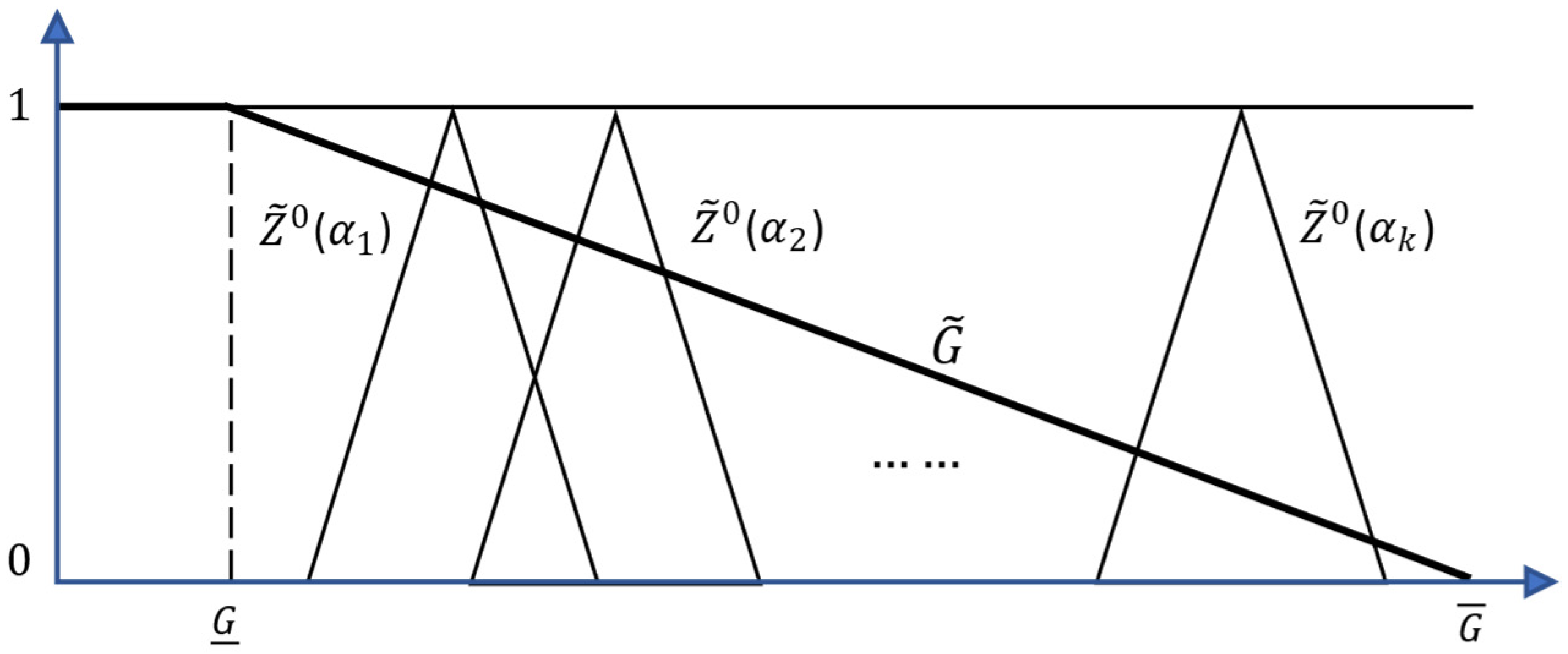In this way, space $\mathcal{O} = \left\{x_0\left({\alpha }_{𝓀}\right),𝜆ϵ\mathcal{M}\right\}$ is obtained from the optimal solution with degree ${\mathsf{\alpha }}_{\mathrm{k}}$ and corresponding possibility distribution with objective value ${\tilde{Z}}^0\left({\alpha }_{𝓀}\right) = \tilde{C}{x}^0\left({\alpha }_{𝓀}\right)$, which is shown in Figure 5.

For acquiring a decision vector that satisfies the decision maker’s expectation, two factors must be considered: (1) the degree of feasibility and (2) reaching the acceptable value for the objective function. After the observation of the obtained information of ${\tilde{\mathrm{Z}}}^0\left({𝒶}_{𝓀}\right)$, the decision-maker is asked to select an objective G and tolerance limit $\overline{\mathrm{G}}$. Accordingly, if $\mathrm{Z}\le \underset{¯}{\mathrm{G}}$, is totally satisfactory; however, if $\mathrm{Z}\ge \overline{\mathrm{G}}$, its satisfaction level is zero. The objective is stated by fuzzy set ${\tilde{\mathrm{Z}}}^0\left({𝒶}_{𝓀}\right)$, whose membership function is as follows:

$${\mu }_G(Z)=\left\{\begin{array}{cc}0\hfill & \mathit{if} Z\le \underset{¯}{G}\hfill \\ \eta \in \left[0,1\right]\hfill & \mathit{decreasing}\begin{array}{c} \mathit{on} \begin{array}{l}\underset{¯}{G}\le Z\le \overline{G}\hfill \end{array}\end{array}\hfill \\ 1\hfill & \mathit{if} Z\ge \overline{G}\hfill \end{array}\right.$$

(71)

The decision-maker wants to acquire the maximum satisfaction level. However, a lower level of constraint establishment is obtained for the optimal objective value. With this explanation, the decision-maker may want a lower level of satisfaction to better establish the constraints. Figure 5 show the different ${\tilde{\mathrm{Z}}}^0$ and objective ${\tilde{\mathrm{Z}}}^0\left({𝒶}_{𝓀}\right)$. The objective is to find a definitive solution $x$* so that the decision maker’ expectation is satisfied.

Stage 2: The satisfaction level of the fuzzy objective ${\tilde{\mathrm{Z}}}^0\left({𝒶}_{𝓀}\right)$ under each optimal solution with acceptance degree α, which the membership function of each fuzzy number ${\tilde{\mathrm{Z}}}^0\left({𝒶}_{𝓀}\right)$ to the fuzzy set ${\tilde{\mathrm{Z}}}^0\left({𝒶}_{𝓀}\right)$ that the method was proposed by [59] is applied here.

$${𝓀}_{\tilde{\mathrm{G}}}({\mathrm{Z}}^0(\mathsf{\alpha }))=\frac{{{\displaystyle \int }}_{-\infty }^{\infty \int }{\mathsf{\mu }}_{{\tilde{\mathrm{Z}}}^0\left(\mathsf{\alpha }\right)}(\mathrm{Z}){\ast \mathsf{\mu }}_{\tilde{\mathrm{G}}\left(\mathsf{\alpha }\right)}(\mathrm{Z})\mathrm{dz}}{{{\displaystyle \int }}_{-\infty }^{\infty \int }{\mathsf{\mu }}_{{\tilde{\mathrm{Z}}}^0\left(\mathsf{\alpha }\right)}(\mathrm{Z})\mathrm{dz}}$$

(72)

In this equation, the dominator identifies the area under the ${\mathsf{\mu }}_{{\mathrm{Z}}^0\left(\mathsf{\alpha }\right)}\left(\mathrm{Z}\right)$ curve and the numerator is the possibility of ${\mathsf{\mu }}_{{\mathrm{Z}}^0\left(\mathsf{\alpha }\right)}\left(\mathrm{Z}\right)$ for any deterministic value Z weighted by its satisfaction level.

Stage 3: We search for finding a balanced solution between the degree of feasibility and satisfaction. Hence, the optimal solution space with acceptance degree α and two fuzzy sets $\tilde{\mathrm{F}}$ and $\tilde{\mathrm{S}}$ is considered, whose membership function is as follows:

$${\mathsf{\mu }}_{\tilde{\mathrm{S}}}\left(x^0({\mathsf{\alpha }}_{𝓀}\right)) = {𝓀}_{\tilde{\mathrm{G}}}\left({\tilde{\mathrm{z}}}^0\left({\mathsf{\alpha }}_{𝓀}\right)\right) \mathrm{and} {\mathsf{\mu }}_{\tilde{\mathrm{F}}}\left(x^0\left({\mathsf{\alpha }}_{𝓀}\right)\right) = {\mathsf{\alpha }}_{𝓀}.$$

(73)

Therefore, the fuzzy decision vector $\tilde{\mathcal{D}}=\tilde{\mathcal{F}}\cap \tilde{\mathcal{S}}$ is defined by [60]:

$${\mathsf{\mu }}_{\tilde{\mathcal{D}}}\left(x^0\left({\mathsf{\alpha }}_{𝓀}\right)\right) = {\mathsf{\alpha }}_{𝓀} \times {𝓀}_{\tilde{\mathrm{G}}}\left({\tilde{\mathrm{z}}}^0\left({\mathsf{\alpha }}_{𝓀}\right)\right)$$

(74)

where * is a $\mathrm{t}-\mathrm{norm}$ that can be minimised. Hence, when we have a deterministic decision vector and, it will be known as a solution for the main fuzzy linear model in Equation (70) if $x^{*}\in O$ is the solution with the most membership degree in the fuzzy decision vectors:

$${\mathsf{\mu }}_{\tilde{\mathcal{D}}}\left(x^{*}\right) = \underset{{\mathsf{\lambda }}_{𝓀}\in \mathcal{M}}{\mathrm{Max}}\left\{{\mathsf{\lambda }}_{𝓀} \times {𝓀}_{\tilde{\mathrm{G}}}\left({\tilde{\mathrm{z}}}^0\left({\mathsf{\alpha }}_{𝓀}\right)\right)\right\}$$

(75)

4. Multi-Objective Metaheuristics Algorithms

Finding optimum solutions to problems that have more than one objective function is difficult [61,62]. Many real-world optimisation problems may pursue different goals, which increases the problem’s complexity [63]. For these challenging problems, metaheuristic algorithms may be used [64]. There are some benefits to using metaheuristic algorithms [65]. They can be applied to any problem that can be expressed as a function optimisation problem [66], are typically easier to understand and implement [67], can solve larger problems faster [68], are simple to design and implement [69], are very flexible [70], and can be combined with other techniques [71]. To the problem in this study, two multi-objective metaheuristic algorithms, NSGA-II [72] and Multi-objective firefly algorithm [73] are employed. The next section delves into the algorithm’s characteristics and pseudo-code.

4.1. NSGA-II

A Non-Dominated Sorted Genetic Algorithm (NSGA-II) is a common and strong method based on the genetic algorithm (GA). Deb, Pratap, Agarwal and Meyarivan [72] proposed this multi-objective algorithm that, instead of a particular solution, identifies a set of solutions as Pareto-front solutions that no one has absolute domination to others. This algorithm is an expert-based multi-objective evolutionary algorithm that maintains the dominant solution with a good strategy and assigns population members by a dominance rank according to non-dominated sorting. Actually, by adding these two important features to the usual genetic algorithm, a set of solutions (i.e., Pareto front) are obtained [74]. Three major operators of this algorithm are selection, mutation and crossover. The selection operator selects the independent parameters among the different parameters to be utilised in mutation and crossover operators. Therefore, setting an appropriate coding is very important to minimise these independent parameters, as the correct selection of genetic operators is also vital for this coding [72] all the duties are done in population generation sections. The crossover and mutation are integrated, then non-dominated sorting is done according to the rank and crowding distance, and finally redundant parts are eliminated [74].

First, a random population of is generated, and each function’s value is computed for each member of the initial population. Following the computation of the objective functions, the non-dominance sorting is applied to the. In this manner, population members with varying degrees of non-domination are classified into several fronts. A non-dominated set of solutions is formed by population members who are not dominated at all (i.e., Pareto front). A secondary measure (namely crowding distance) is used to sort solutions that have the same rank and are in the same non-dominance level. This crowding distance for solution I is an estimate of the diameter of a rectangle, the vertices of which are the closest neighbour solutions to it in its front. The crossover operator is applied to a subset of the current population at each iteration, and new solutions are generated. Each member of the new population is given the value of each objective function. To select parent solutions, a binary tournament selection was used. Algorithm 1 presents the steps of any iteration of the NSGA-II. When a user-specified number of iterations is reached, the algorithm is completed.

Algorithm 1: NSGA-II Algorithm.
	Initialization of generation $A_{\xi }$;
	Initialization of iteration $\xi =1$;
	while generation $\xi \le {\xi }_{max}$
		Crossover and mutation on $A_{\xi }$ to get new population $B_{\xi }$;
		Merge $A_{\xi }$ and $B_{\xi }$ as total population $T_{\xi }$;
		Rank population $T_{\xi }$ in Pareto front;
		Select best $N_p$ population from $T_{\xi }$ as $A_{\xi +1}$ with crowding distance function;
		Increment generation $\xi =\xi +1$
	end

4.2. Multi-Objective Firefly Algorithm

Firefly algorithm was proposed by Yang [75]. The fireflies generate short and rhythmic flashes (with unique pattern) the flashing light is generated by a procedure of bioluminescence [76]. With chemical changes in them, these insects flash to attract a mating partner or protect themselves. There are three rules in this algorithm, which are as follows:

• A firefly can attract another firefly regardless of their gender (all fireflies are unisex).
• The brighter firefly attracts the other one (the dependence of attraction rate of fireflies to their brightness). The brightness and attractiveness increase with distance reduction.
• The more bright the firefly is, the more objective function it has. Thus, the obtained solution will be better. To find the brightness value of these insects, we can use the objective function [77]. In other words, the objective function of this algorithm is the same as the fitness function of the genetic algorithm [78].

To better understand this concept, consider that the butterfly’s attractiveness is defined by its brightness. For a maximisation problem, the brightness (illumination) of a firefly ($\mathrm{I}$) located at point x is equivalent to $\mathcal{I}\left(x\right)\propto 𝒻\left(x\right)$ [75]. The attractiveness is relative meaning that other fireflies should judge it. So, it will differ with the distance of two fireflies i and j ($r_{ij}$). By this explanation, the firefly attractiveness is obtained from the following equation:

$$\mathsf{\beta }\left(𝓇\right) = {\mathsf{\beta }}_0{\mathrm{e}}^{ - \mathsf{\gamma }{𝓇}^2}$$

(76)

where ${\mathsf{\beta }}_0$ is the initial attractiveness of firefly at distance $𝓇$ = 0. In more detailed explanation, this equation identifies that at a given distance $ℾ = 1/\sqrt{\mathsf{\gamma }}$, the attractiveness changes remarkably from ${\mathsf{\beta }}_0$ to ${ \mathsf{\beta }\mathrm{e}}^{-1}$. The distance of two fireflies is located at points $x_i$ and $x_{𝒿}$. $x_{i,𝓀}$ is the k-th factor of the spatial coordinates of the i-th firefly. Of course, with regard to the research problem’s nature, other metrics (e.g., Manhattan distance or Mahalanobis distance) can be considered for identifying the distance [79]. If $\mathsf{\gamma }\to 0, \mathsf{\beta }={\mathsf{\beta }}_0$; hence the firefly’s attractiveness value is close to zero (if that is seen by other firefly) if $\mathsf{\gamma }\to \infty , \mathsf{\beta }=0$. That means any firefly moves in the random route and the other firefly has not seen [80]. If the firefly i is attracted to the brighter firefly j, its movement is calculated by [73].

$$x_i^{𝓉+1}=x_i^{𝓉}+{\beta }_0\times e^{-\gamma {𝓇}_{i𝒿}^2}\times \left(x_{𝒿}^{𝓉}-x_i^{𝓉}\right)+{\alpha }_{𝓉}\times {ϵ}_i^{𝓉}$$

(77)

The second statement identifies the attractiveness, and the third statement has been randomised with random parameter ${\alpha }_{𝓉}$ (randomisation) and ${ϵ}_i^{𝓉}$ is the produced vector of Gaussian or Uniform distribution function. This statement generates random number with control parameter ${\mathsf{\alpha }}_{\mathrm{t}}$ that the most applicable parameters value is when ${\mathsf{\beta }}_0=1$ and $\in \left[0,1\right]$. By this explanation, the following equation can be written.

$$x_i^{𝓉+1}=x_i^{𝓉}+{\beta }_0\times e^{-\gamma {𝓇}_{i𝒿}^2}\times \left(x_{𝒿}^{𝓉}-x_i^{𝓉}\right)+{\mathsf{\alpha }}_{𝓉}\times \left(\mathrm{rand}-\frac{1}{2}\right)$$

(78)

In conclusion, it can be said that four stages are designed for applying this algorithm. In Stage 1, the generation of an initial population of fireflies is taken place. Then, their fitness or light intensity is evaluated to the objective function. In Stage 3, this fitness value is updated. In the final stage, the fireflies are ranked, and their states are updated. [73] developed the original FA for multi-objective problems by applying three rules and characteristics. Actually, this algorithm is the adjusted firefly algorithm [81]. According to the emitted light from firefly, this algorithm reproduces the attractiveness rate between them. Therefore, the brightest firefly attracts at least one firefly. In the optimisation problem, each firefly represents a solution to the problem, and the lighter firefly has better quality [82]. The pseudo-code of the multi-objective firefly algorithm (MOFA) can be explained in two stages. As shown in Algorithm 2, in the first stage, after the completion of initialisation, the first firefly that is less bright moves to the brighter one. In other words, all fireflies are compared to fireflies that are smaller than or equal to them by ε, and if one of them dominate others by ε, the firefly with the least brightness approaches the brightest one. if the obtained firefly is better than the original firefly with respect to dominance, it is replaced with it. In fact, in this stage, the moved fireflies to the better ones are counted to identify whether the population has encountered with stagnant or not. The times in which fireflies have encountered stagnant have unsuccessful attempts for evolution. In the second stage, it is identified whether the population is being encountered with stagnant or not. According to the moved fireflies and their limit values, when the number of fireflies approached to the brighter one is less than StageCont, the population is deemed to be stagnated and if their limit values are greater than LimitF, replaced with new random fireflies. At the end of each generation, the validated members of the population are stored in DS Archive to new appropriate solutions [82].

Algorithm 2: MOFA.
NF$\leftarrow$Number of fireflies.
NDS Archive$\leftarrow$∅
# Initialization.
Fireflies$\leftarrow$Generate NF random fireflies.
Generations$\leftarrow$Number of iterations of the algorithm.
Fmoved$\leftarrow$Number of fireflies moved in each generation.
StagCont$\leftarrow$Percentage of fireflies for stagnation control.
LimitF$\leftarrow$Maximum number of times that a firefly tries unsuccessfully to evolve.
fori = 1 to generations
	# Evolution of the swarm
	Fmoved$\leftarrow$0
	for j = 1 to NF
		FireflyA$\leftarrow$ Fireflies[j]
		for k = 1 to NF
			fireflyB$\leftarrow$ fireflies[k]   #fireflyB≠fireflyA
			if fireflyA ${\preccurlyeq }_{\epsilon }$ fireflyB
				fireflyR$\leftarrow$ bringcloser(fireflyB,firefly)
				if fireflyR $\prec$ fireflyB
					Fireflies[k]$\leftarrow$ fireflyR
					Fmoved$\leftarrow$ Fmoved +1
				else
					incrementLimit(Fireflies[k],1)
				end
			end
		end
	end
	# Stagnation Control
	if Fmoved < (NF$\times$ StagCont)/100
		for m = 1 to NF
			if limit (fireflies[m]) > LimitF
				Fireflies[m]$\leftarrow$ newrandom firefly.
			end
		end
	end
	# Save population to the NDSArchive.
	export fireflies (fireflies,NF,NDSArchive)
end

5. Computational Results

The results are shown in the following four sub-sections.

5.1. Evaluating the Performance of the Algorithms

Ten problems in different dimensions are designed to compare the proposed meta-heuristic algorithms (i.e., NSGA-II and MOFA). We compare the obtained results of these meta-heuristics with the GAMS’s results obtained by the augmented ε-constraint method. As shown in

Table 4. The best values of the augmented ε-constraint method, NSGA-II and MOFA.

(Problem No., Depots, Affected Areas)	Augmented ε-Constraint		NSGA-II		Gap (%)	MOFA		Gap (%)
	$(\mathit{O}{\mathit{F}}_1$$,\mathit{O}{\mathit{F}}_2$$, \mathit{O}{\mathit{F}}_3)$	Time	$(\mathit{O}{\mathit{F}}_1$$,\mathit{O}{\mathit{F}}_2$$, \mathit{O}{\mathit{F}}_3)$	Time	$(\mathit{O}{\mathit{F}}_1$$,\mathit{O}{\mathit{F}}_2$$, \mathit{O}{\mathit{F}}_3)$	$(\mathit{O}{\mathit{F}}_1$$,\mathit{O}{\mathit{F}}_2$$, \mathit{O}{\mathit{F}}_3)$	Time	$(\mathit{O}{\mathit{F}}_1$$,\mathit{O}{\mathit{F}}_2$$, \mathit{O}{\mathit{F}}_3)$
(1, 2, 5)	(24.7, 3.4, 13.1)	147	(24.8, 3.4, 13.2)	249	(0.004, 0.000, 0.008)	(24.7, 3.4, 13.1)	387	(0.00, 0.00, 0.00)
(2, 3, 10)	(27.4, 4.7, 14.2)	261	(27.9, 4.4, 14.4)	327	(0.018, 0.064, 0.014)	(27.4, 4.7, 14.2)	492	(0.00, 0.00, 0.00)
(3, 4, 9)	(28.9, 3.8, 14.9)	392	(30.1, 3.7, 15.6)	586	(0.042, 0.026, 0.047)	(29.3, 3.7, 15.4)	719	(0.014, 0.026, 0.034)
(4, 3, 12)	(30.7, 6.1, 16.8)	504	(31.2, 5.5, 17.5)	765	(0.016, 0.098, 0.042)	(30.9, 5.8, 17.1)	963	(0.007, 0.049, 0.018)
(5, 5, 14)	(34.1, 6.4, 15.3)	793	(35.9, 6.1, 16)	980	(0.053, 0.047, 0.046)	(35, 6, 15.9)	1104	(0.026, 0.063, 0.039)
(6, 6, 15)	(43.6, 5.7, 16.1)	947	(56.2, 5.3, 16.6)	1297	(0.060, 0.070, 0.031)	(45.9, 5.4, 16.7)	1284	(0.053, 0.053, 0.037)
(7, 7, 17)	(48.2, 6.2, 15.8)	1297	(51, 5.9, 16.4)	1753	(0.058, 0.048, 0.038)	(49.3, 5.8, 16.2)	1403	(0.023, 0.065, 0.025)
(8, 8, 18)	(56, 8.1, 14.2)	1696	(58.2, 7.7, 14.9)	2102	(0.039, 0.049, 0.049)	(58.4, 7.7, 14.5)	1883	(0.043, 0.049, 0.021)
(9, 9, 19)	(-, -, -)	-	(69.8, 8.4, 17.3)	2683	(-, -, -)	(70.1, 8.3, 17)	2292	(-, -, -)
(10, 10, 21)	(-, -, -)	-	(81, 9.6, 16.8)	3103	(-, -, -)	(80.8, 9.8, 17.1)	2841	(-, -, -)
Average	(36.7, 5.55, 15.05)	754.625	(45.61, 6, 15.87)	1093.8	(3.58, 5.06, 3.22)	(45.18, 6.06, 15.72)	1336.8	(1.75, 3.64, 2.19)

, for each produced problem, the values of Objective Function (OF) and errors of the proposed meta-heuristics are reported in comparison to the augmented ε-constraint method, in which the solution time of this method is at most 3600 s. In this paper, for each of the three objective functions of the mathematical model, the error rate of each algorithm in comparison to the $\mathrm{Augmented}$ ε-constraint method can be calculated from the following equations (for the calculation of the MO-firefly algorithm’s error, we do similarly).

$${\mathrm{Gap}}_{O{F}_i}=\frac{O{F}_i{}_{\mathrm{NSGA}\text{-}\mathrm{II}}-O{F}_i{}_{\mathrm{Augmented} \mathsf{\epsilon }\text{-}\mathrm{Constaint}}}{O{F}_i{}_{\mathrm{Augmented} \mathsf{\epsilon }\text{-}\mathrm{Constaint}}}\times 100,\hspace{1em}i=1,2,3$$

(79)

The mean differences between the NSGAII and augmented ε-constraint method values are 3.58, 5.06 and 3.22% for the first, second and third objective functions (i.e., transportation time, reliability and unmet demand or shortage), respectively. Furthermore, the mean differences between the best values of the MOFA and $\mathsf{\epsilon }$-constraint method are 1.75, 3.64 and 2.19% for the first, second and third objective functions, respectively. As a result, we infer that the suggested metaheuristic approaches are efficient since the mean gaps of three objective functions are quite small (see Figure 6).

Furthermore, Figure 7 compares the CPU time of the augmented ε-constraint method to the time required to solve each of the meta-heuristic algorithms. As the dimensions of the problem increase, the solving time of the augmented ε-constraint method increases exponentially, to the point where it cannot solve problems 9 and 10. In contrast, the proposed metaheuristic algorithms can find good solutions in a reasonable amount of time and with a reasonable slope.

5.2. Evaluating Metrics and Comparing Three Objectives Meta-Heuristics

To compare the performance of different algorithms in multi-objective optimisation problems, in which problem solutions constitute the optimal Pareto front, there are different criteria used in this research. One quantitative criterion of algorithms’ performance is the number of Pareto solutions, in which higher values of this number indicate that it is more appropriate. On the other hand, the distance index can be used to calculate the relative distance of consecutive solutions. The lower values of this index are more desirable. This distance index is calculated by [83].

$$SM = \frac{{{\displaystyle \sum }}_{i = 1}^{\mathcal{N} - 1}\left|\overline{𝒹} - {𝒹}_i\right|}{\left(\mathcal{N} - 1\right)\overline{𝒹}}$$

(80)

where $N$ is the number of Pareto solutions, ${𝒹}_i$ is the spacing between two sequential solutions in optimal front obtained by each algorithm, and $𝒹$ is the average of $dis$. Another index that identifies the diversity of solutions is the diversity index, in which its higher values are more appropriate. This index can be computed by [84]:

$$DM = \sqrt{{\left(\frac{max{𝒻}_{1i} - min{𝒻}_{1𝒾}}{{𝒻}_{1,total}^{max} - {𝒻}_{1,total}^{min}}\right)}^2 + {\left(\frac{max{𝒻}_{2i} - min{𝒻}_{2i}}{{𝒻}_{2,total}^{max} - {𝒻}_{2,total}^{min}}\right)}^2}$$

(81)

To compare the performance of the proposed algorithms and generate Pareto-optimal solutions, 12 problems with different sizes are produced and the evaluation metrics of two meta-heuristic algorithms are presented for each problem. The attributes of the generated sample problems, the failure times, the fuzzy demands for vehicles under different scenarios and values of evaluations metrics for algorithms are given in

Table 5. Characteristics of generated sample problems.

Problem No.	Helicopter	Truck	Vehicle Depot	Impacted Area in Cluster 2	Impacted Area in Cluster 1
1	2	3	6	5	7
2	2	3	6	7	10
3	2	4	8	9	15
4	2	4	7	7	16
5	3	5	7	8	18
6	3	6	8	8	20
7	3	6	8	10	24
8	4	5	9	11	25
9	4	7	9	15	30
10	5	7	9	16	33
11	5	9	9	20	35
12	5	9	10	30	40
13	5	10	12	30	45
14	5	10	15	35	50

,

Table 6. The failure times and fuzzy demand for vehicles under different scenarios.

$\widetilde{\mathit{d}\mathit{e}{\mathit{m}}_{\mathit{i}}}$			Vehicle
$\widetilde{dem}=\left(de{m}_1,de{m}_2,de{m}_3\right)$	5	4	3	2	1	scenario
(20, 46, 75)	10	16	13	7	10	1
(25, 50, 80)	10	9	14	4	20	2
(30, 53, 95)	16	8	11	16	10	3
(35, 60, 100)	10	20	7	10	10	4
(45, 70, 120)	8	10	9	10	15	5

and

Table 7. Values of evaluations metrics for NSGAII and MOFA.

Problem No.	NSGA-II				Firefly
	SM	DM	NOPS	Run Time	SM	DM	NOPS	Run Time
1	0.914	7.2881	7	612	0.5922	7.6371	14	645
2	0.7145	5.6559	6	754	0.8038	5.1245	9	763
3	1.0176	6.9782	6	1021	0.9946	5.5324	10	998
4	0.3557	7.5087	8	1213	0.465	7.1512	8	1168
5	0.9968	3.8052	6	1627	0.499	6.9166	7	1455
6	0.5547	4.8781	12	1871	0.6264	3.4117	9	1666
7	1.085	3.1801	5	2580	0.4833	3.0387	9	2224
8	0.5612	4.9553	6	2915	1.0506	4.1797	8	2443
9	0.9063	5.6559	8	3987	0.4396	8.4969	14	3496
10	0.726	7.9399	7	5758	0.7331	6.4724	11	5404
11	0.8614	6.7129	7	7108	0.8054	7.9225	14	6337
12	0.5916	7.8599	6	10,049	0.4164	7.4799	11	8223
Average	0.7737	6.0349	7	3291.8333	0.6591	6.1136	10.3333	391.0351

.

It’s important to note that the number of ground vehicles is between 3 and 10, and the number of air vehicles is between 2 and 5. In all problems, there is one warehouse for air vehicles. Also, the capacity and transportation time parameter values are generated according to a uniform distribution U (50, 60) and U (8, 20), respectively. The demand of affected people is considered a triangle fuzzy number with the $dem = \left(de{m}_1,de{m}_2,de{m}_3\right)$ structure, which generate randomly as follows (from Uniform distribution): dem₁ from [20,45], dem₂ from [46,70], and dem₃ from [71,140]. The travel time of vehicles for distributing goods is also considered a uniform distribution, which a part of this generated random numbers can be seen in Table 6. For each problem, we have a scenario matrix, in which the rows identify scenarios, the columns identify vehicles, and the numbers in the table identify the failure time of vehicles. That is ${\mathrm{scenario}}_2^3 = 16$ highlighted in the table meaning that vehicle 2 in scenario five is broken down after 16 h and causes the unmet demand. Finally, Table 7 shows the comparison of the two proposed meta-heuristic algorithms.

The computational results of comparison metrics are shown below for a better understanding of the performance of the meta-heuristic algorithms. We compare the meta-heuristic algorithms in Figure 8 using the distance metric and find that the MOFA outperforms the NSGA-II. The density metric results in Figure 9 show that there is no special trend for the algorithms. Figure 10 depicts the number of Pareto solutions demonstrating the MOFA’s superior performance. Figure 11 depicts a comparison of solution times, demonstrating that the MOFA is faster in finding good solutions, resulting in better performance.

5.3. Sensitivity Analysis

The sensitivity analysis is considered for problem 6 (i.e., 28 impacted areas, eight warehouses, nine vehicles and five scenarios). The results of the objective functions are changed in demand and vehicle capacity simultaneously, and the mean of the vehicle damage time (parameter of exponential distribution in scenarios generation) is shown in

Table 8. Sensitivity analysis of the changes in vehicle capacity and demand functions simultaneously.

Capacity				Demand
	0.7			0.8			0.9			1			1.1			1.2			1.3
	$\mathit{O}{\mathit{F}}_1$	$\mathit{O}{\mathit{F}}_2$	$\mathit{O}{\mathit{F}}_3$	$\mathit{O}{\mathit{F}}_1$	$\mathit{O}{\mathit{F}}_2$	$\mathit{O}{\mathit{F}}_3$	$\mathit{O}{\mathit{F}}_1$	$\mathit{O}{\mathit{F}}_2$	$\mathit{O}{\mathit{F}}_3$	$\mathit{O}{\mathit{F}}_1$	$\mathit{O}{\mathit{F}}_2$	$\mathit{O}{\mathit{F}}_3$	$\mathit{O}{\mathit{F}}_1$	$\mathit{O}{\mathit{F}}_2$	$\mathit{O}{\mathit{F}}_3$	$\mathit{O}{\mathit{F}}_1$	$\mathit{O}{\mathit{F}}_2$	$\mathit{O}{\mathit{F}}_3$	$\mathit{O}{\mathit{F}}_1$	$\mathit{O}{\mathit{F}}_2$	$\mathit{O}{\mathit{F}}_3$
0.7	43.6	5.7	12.9	43.6	5.7	14.2	45.2	5.6	16.7	48.2	5.6	17.7	50.1	5.4	18.4	54.3	5.3	19.2	59.4	5.2	20.2
0.8	43.6	5.7	12.9	43.6	5.7	14.2	43.6	5.7	15.4	44.9	5.6	16.9	46.3	5.5	17.8	48.7	5.3	18.2	55.1	5.2	19.5
0.9	43.6	5.7	12.9	43.6	5.7	14.2	43.6	5.7	15.4	43.6	5.7	16.1	46.5	5.7	17.1	47	5.6	17.8	51.3	5.4	18.8
1	43.6	5.7	12.9	43.6	5.7	14.2	43.6	5.7	15.4	43.6	5.7	16.1	43.6	5.7	16.4	47.1	5.7	17.3	49.7	5.6	18.3
1.1	43.6	5.7	12.9	43.6	5.7	14.2	43.6	5.7	15.4	43.6	5.7	16.1	43.6	5.7	16.4	43.6	5.7	17.3	46.5	5.6	18
1.2	43.6	5.7	12.9	43.6	5.7	14.2	43.6	5.7	15.4	43.6	5.7	16.1	43.6	5.7	16.4	43.6	5.7	17.3	43.6	5.7	17.7
1.3	43.6	5.7	12.9	43.6	5.7	14.2	43.6	5.7	15.4	43.6	5.7	16.1	43.6	5.7	16.4	43.6	5.7	17.3	43.6	5.7	17.7

and

Table 9. Sensitivity analysis of the changes mean of vehicle damage time.

Mean of Vehicle’s Damage Time	0.3	0.4	0.5	0.6	0.7	0.8	0.9	1	1.1	1.2	1.3	1.4	1.5
$\mathit{O}{\mathit{F}}_{\mathbf{1}}$	51.8	51.6	50.9	49.3	49	44.6	43.8	43.6	43.4	40.2	39.5	39.3	37.2
$\mathit{O}{\mathit{F}}_{\mathbf{2}}$	5.2	5.2	5.3	5.4	5.4	5.6	5.7	5.7	5.7	5.8	5.8	5.8	5.9
$\mathit{O}{\mathit{F}}_{\mathbf{3}}$	19.3	19.3	19.4	19.1	18.5	17.8	17	16.1	15.3	14.7	14.1	13.9	13.9

.

If the demand reducing and vehicle capacity increasing simultaneous then will be no change in the route selection and objective functions. Vice versa, when demand increases and a capacity decrease, then the transportation times (OF1) and unmet demand (OF3) will be increased, and the reliability (OF3) will be decreased. Because of rising demand and low capacity to serve more vehicles need (OF1). Therefore, the increased transportation time and vehicle failure probability will be increased. As a result, the unmet demand (OF3) increases, on the other hands; the route selection with lower reliability will be increased. If demand is fixed and the vehicle capacity is decreased, it sounds like, we reduce surplus capacity. Thus, route selection does not change. But when the demand constant and the vehicle capacity decrease from 0.9 to 0.8, the three objective functions will be changed. Thus, the routes change. For example, if vehicle 1 should serve three impacted areas, now because of decrease its capacity will not be able to serve, therefore this task will be devolved to vehicle 2. When vehicle 2 transports the arc, firstly, transportation time (OF1) increases, and it is not optimal. Secondly, the unmet demand value (OF3) in different scenarios increases. Thirdly, the arc with the most reliability is selected before, but now, the reliability decreases from 5.7 to 5.6. Similarly, if the vehicle capacity decreases up to 0.7, this change will be had again. Now, if the vehicle capacity is considered constant (value = 1) and demand decreases, the route and objective functions will not change. However, if demand increases then because of constant capacity and increased demand, the vehicle cannot response this demand volume. As a result, the transportation time will be increased and reliability will be decreased on the other hands, the vehicle damaged under different scenarios, therefore the unmet demand value will be increased. The results of vehicle downtime and its impact on the optimal solution is shown in Table 9. According to what is shown in Table 7, we find if the mean of the damage time increases, the characteristic related to vehicle damage times will be decreased. When damage time is increased (from 1 to 1.1), the vehicle performs better, transportation time increases, reliability increases, and unmet demand decrease. The model or algorithm tries to do, not selected routes where the vehicle broken-down earlier and there has the unmet demand value. Vice versa, if the mean of the damage time is decreased until the vehicle breaks down sooner, the model tries to increase the mean of the damage time. In fact, the model is increased both of the unmet demand value and transportation time.

5.4. Practical Implication

There are many cities in the world that are in high-risk areas, and the original designs of many hospitals failed to account for the potential effects of natural disasters on the built environment. Despite the fact that natural disasters are extremely rare, it is imperative to have a plan in place for dealing with them. As a result of this research, some government organisations and decision-makers may be able to develop a central platform for distributing temporary shelters to impacted areas. There are also a number of international organisations that are working on solutions for displaced people. Global campaigns have been launched by organisations like the WHO and the United Nations International Strategy for Disaster Reduction. As a result of this study, a Graphical User Interface (GUI) for emergency planning organisations can be developed using the model proposed. An online visualisation prototype that generates reliable and dynamic response plans quickly would be extremely helpful to strategic and operational planners. Decision-makers may benefit from the prototype’s ability to speed up the evacuation planning process. It will have an easy-to-use data input system that can generate a lot of data for this decision-making tool. Effective disaster response plans that can be modified quickly and easily in the event of a disaster may be possible with this information.

6. Conclusions and Future Research

As the destructive impacts of disasters on societies and built environments are predicted to increase in the future, innovative disaster response strategies to cope with emergency conditions are be-coming more crucial. Due to time and resource constraints after a distractive large-scale disaster, the distribution of post-disaster temporary shelters is challenging. There is strong evidence that the success of many post-disaster response strategies in providing temporary shelters for impacted areas is compromised by inappropriate planning. In this research, by proposing a clustered and disrupted vehicle routing model, we tried to minimise the total travel time of operations and the unmet demand (shortage) and maximise the reliability of the route simultaneously. A system was designed in which heterogeneous vehicles from multiple depots initiated the relief operations in the ground and air mode and delivered temporary shelters to the impacted areas. The augmented ε-constraint method in small size was used to find the optimal solution. To compare the performance of the proposed algorithms and generate the optimal solution, 12 problems with different sizes were produced, and the evaluation metrics of two meta-heuristic algorithms were presented for each problem. The results identified higher accuracy and lowered computational time of the multi-objective firefly algorithm.

This research has implications for key stakeholders involved in disaster management strategies and plans in disaster-prone areas, according to the empirical findings. Furthermore, policymakers in disaster-stricken countries can use the proposed model to manage emergency situations. In addition, the proposed model can be easily adapted to other disasters, such as bushfires, which are common in many countries, particularly Australia. Using a bushfire simulation framework like “Spark” developed by CSIRO-Data61, bushfire spread across the landscape can be predicted, allowing the availability of different network links to be estimated.

It is possible to extend this study in many ways. As an example, incorporating staff scheduling and management into the distribution process could be an interesting research area. In the future, researchers should look into how well the road network performs when distributing shelters. In addition, disaster response can be more efficient and time-saving if interrelated operations are coordinated. As a result, developing multi-category integrated models could be an exciting new area of study in the future.