The Mechanism of Influencing Green Technology Innovation Behavior: Evidence from Chinese Construction Enterprises

Abstract

The Green Technology Innovation Behavior (GTIB) of construction enterprises is crucial for promoting green development in the construction industry. In order to clarify the mechanism of action affecting the GTIB of construction enterprises, this paper considers the context of green development in the construction industry based on the vector autoregressive model and constructs a theoretical model of GTIB in construction enterprises. Time series data collected by the Chinese government (2000–2018) were used to analyze the mechanism of action of the factors influencing the GTIB of construction enterprises by EViews 10.0. The results of the paper showed the following: (1) direct government investment has the greatest impact on the GTIB of construction enterprises and has made a positive contribution; (2) the added value of Gross Domestic Product (GDP) of the construction industry has a relatively small impact on the GTIB of construction enterprises; (3) the role of environmental regulation on the GTIB of construction enterprises is non-linear. This paper further broadens the research to the factors influencing the GTIB of construction enterprises. Meanwhile, this paper provides a reference basis for local governments to formulate policies related to the GTIB of construction enterprises.

1. Introduction

As the process of globalization continues to accelerate, environmental issues are becoming more and more serious [1]. Although the construction industry is an important part of the national economy of countries around the world [2], its production activities have been accompanied by high consumption, serious pollution, crude construction methods and serious pollution, etc. [3]. Therefore, many countries have proposed to renovate existing buildings with high energy consumption and poor functionality [4]. In the field of construction technology innovation, patents have been paid attention by countries and regions all over the world. As of 2018, there are 158,471 building patents in the United States (US), 59,891 in the Britain, 89,586 in France, 163,542 in Germany and 92,634 in Japan [5]. Although construction technology innovation in the US, Britain, France, Germany, and Japan has already established a scale, compared with general patents, the number of green building-related patents across the world is very limited. In other words, for the entire construction industry, there is still more room for growth in the green technology innovation of construction enterprises.

Although, as of 2018, the number of construction patents in China reached 362,063 [6], China’s green building and the green technology innovation behavior (GTIB) of its construction enterprises are still in their early stages compared with developed western countries [7]. To address the environmental issues brought about by the process of economic growth, green development as a complex adaptive system integrating policy, life, production and human and natural life communities has become something that has received substantial attention from academia and industry [8]. Not only in agriculture, but also in the production and operation management of industrial enterprises, such organizational behavior as green development behavior is generated [9]. In particular, the production activities of construction companies are equally inseparable from green development, e.g., in the remanufacturing supply chain of construction waste, the role of technological innovation cannot be ignored [10,11,12]. The GTIB of construction enterprises is a kind of green development behavior, and the main body of this behavior is construction enterprises. In other words, the GTIB of construction enterprises is a technical innovation behavior that is beneficial to their own economic development and environmental protection that helps them achieve their green development goals. Thus, it is important for the sustainable development of the construction industry to conduct an in-depth study of the mechanism of the GTIB of construction enterprises and propose countermeasures.

In order to clarify the mechanism of action affecting the GTIB of construction enterprises, this paper considers the background of green development in construction industries based on VAR model and constructs a theoretical model of each factor of the GTIB of construction enterprises. This paper is tested empirically using time series data collected by the Chinese government for the period 2000–2018. As far as we know, no scholars have yet conducted a systematic analysis on this.

2. Literature Review

From the perspective of influencing factors, the existing research literature can be divided into the following three categories.

In general, governmental actions have been an important factor influencing the development of the industry [13]. Meanwhile, Chang et al. [14] pointed out that the incentive policies set by governments can promote the application of renewable energy in the construction of buildings and infrastructure. Therefore, this paper proposes the following hypothesis:

Hypothesis 1 (H1).

Direct government investment has a significant positive effect on the GTIB of construction enterprises.

At the same time, because the GTIB of construction enterprises is part of construction technology innovation, it will also be influenced by the size of the construction enterprises [15]. In the early stages, when the scale of the construction industry was small, the green technology innovation of construction enterprises was also relatively insignificant. At a later stage, as the scale of the construction industry increased, the GTIB of construction enterprises also developed accordingly. The development of the scale of the construction industry has improved the awareness of green innovation of construction enterprises, thus promoting the GTIB of construction enterprises. On the basis of the above theoretical analysis, the second hypothesis is proposed in this paper.

Hypothesis 2 (H2).

The industrial scale of construction enterprises has a long-term, stable and positive impact on the GTIB of construction enterprises.

Some of the existing studies of the effect of environmental regulation on the GTIB of construction enterprises have concluded that there is a positive effect of environmental regulation on the GTIB of construction enterprises [16], while others have concluded that environmental regulation hinders the development of the GTIB of construction enterprises [17]. In its early stages, environmental regulation has a positive effect on green innovation in construction enterprises. In the later stage, as the number of environmental regulations increased, the GTIB of construction enterprises also decreased gradually. Based on the above analysis, the third hypothesis is proposed in this paper.

Hypothesis 3 (H3).

The impact of environmental regulations on the GTIB of construction enterprises is non-linear.

In summary, it can be seen that, although there has been a large amount of literature on green building technology innovation and its influencing factors, the empirical research on the influencing factors of the GTIB development level of construction enterprises has not been sufficient. At the same time, previous studies tend to study the influence on the development of the GTIB of construction enterprises only from a single perspective as well as to study the influence of the corresponding policies formulated by the government on the GTIB of construction enterprises. The results of these studies generally suggest that the factors that promote the development of the GTIB of construction enterprises are mainly government incentives, mature markets, lower costs and the interest of enterprises in green building technology (GBT), while the factors that hinder the development of the GTIB of construction enterprises are generally considered to be the lack of awareness of GBT and the excessive costs of adopting GBT. However, most of these studies have focused on the adoption factors of GBT. In this paper, based on the previous studies, the influence of the governmental behavior factor, the science and technology investment factor, the industry scale factor and the urban construction development factor on the level of the GTIB of construction enterprises are considered comprehensively. Meanwhile, this study introduces a VAR model by constructing a new model of green innovation behavior of construction enterprises, and analyzes the mechanism of action affecting the GTIB of construction enterprises through impulse response function analysis, variance decomposition analysis, co-integration test and Granger causality.

3. Methods and Indicators

3.1. Methods

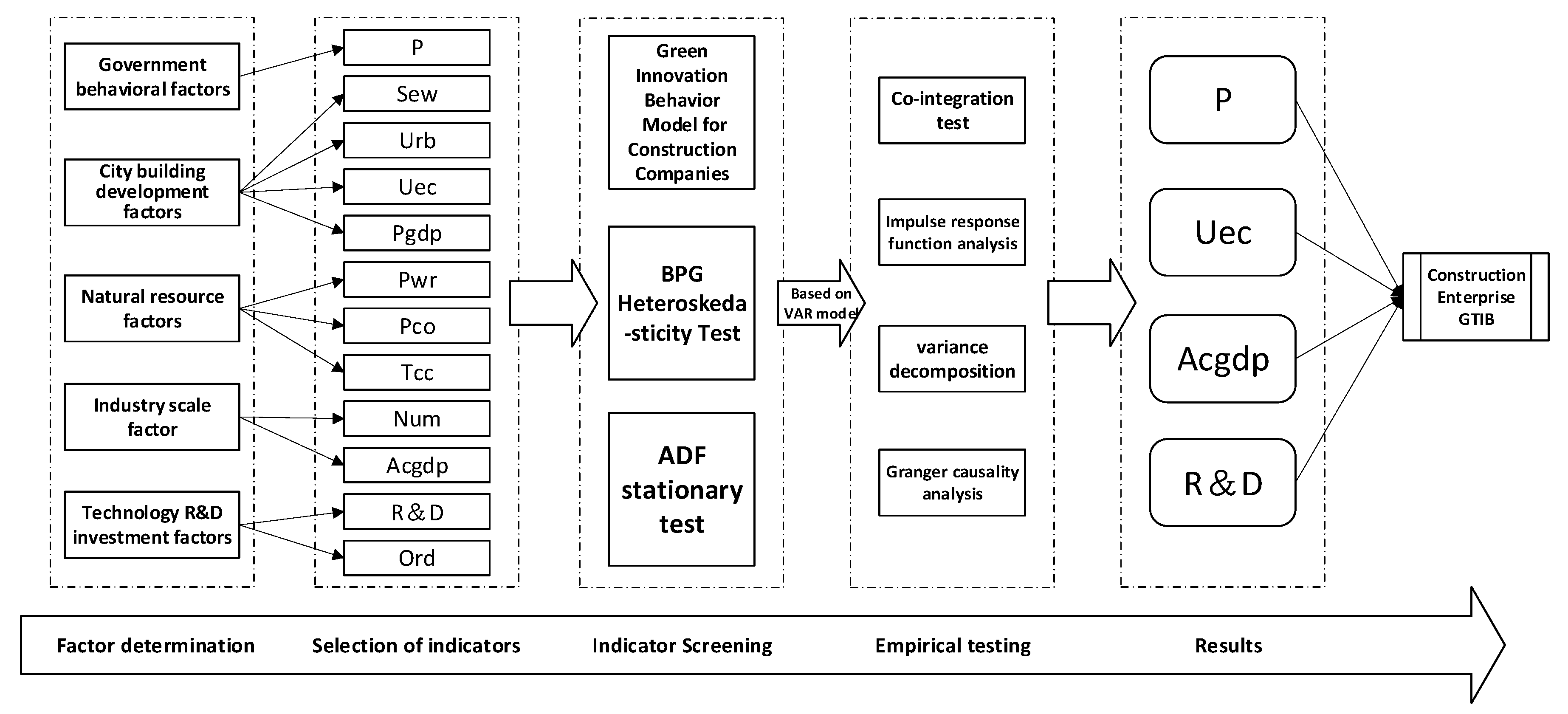
In order to achieve the research objective, this paper analyzed the mechanism of action affecting the GTIB of construction enterprises based on various data of the national time series from 2000 to 2018, applying multiple linear regression models, VAR models and various analytical methods with EViews 10.0. At the same time, this paper draws a technical roadmap of influencing factors based on the GTIB model of construction enterprises in order to clearly show the mechanism of action affecting the GTIB of construction enterprises, as shown in Figure 1.

3.1.1. Multiple Linear Regression

The main purpose of the multivariable linear regression model (MLR) is to explain and predict the relationship between the dependent variable and multiple independent variables [18]. A phenomenon is usually influenced by several external factors, and it is more effective and realistic to predict or estimate the dependent variable by the optimal combination of several independent variables together at the same time, rather than by just one independent variable. In this paper, therefore, a model of GTIB in the construction industry is constructed, i.e., a multiple linear regression (MLR) model is used to analyze the correlation between the level of GTIB development in construction enterprises and other variables. The general form of this is Equation (1).

y_t = β₀x + β₁x_1t + β₂x_2t + … + β_kx_kt + u_t   t = 1, 2, …, T

(1)

where k is the number of explanatory variables and β_j (j = 1, 2, …, k) is called the regression coefficient. Equation (1) is also known as the stochastic expression for the overall regression function.

Therefore, a multiple linear regression model can be used to analyze the mechanism of action affecting the GTIB of construction enterprises, and the model is shown in Equation (2).

PT = c₁ × R&D + c₂ × Sew + c₃ × Acgdp + c₄ × Pgdp + c₅ × Uec + c₆ × P + c₇ × Num + c₈ × Urb + c₉ × Pco + c₁₀ × Tcc + c₁₁ × Ord + c₁₂ × Pwr + C

(2)

where PT is the number of green building patents, P is the number of environmental protection policies, Pgdp is Gross Domestic Product (GDP) per capita, Uec is the amount of urban environmental infrastructure construction investment, Sew is the sewage treatment rate, R&D is the amount of capital invested in research and development, Acgdp is the value added of construction production, Num is the number of construction enterprises, Urb is the national urbanization rate, Pco is cement production per capita, Pwr is Water resources, Tcc is total energy consumption in the construction industry, Ord is the number of undergraduate enrolment and c_j (j = 1, 2, …, 7) is called the regression coefficient.

3.1.2. Vector Autoregressive (VAR) Model

Vector autoregressive (VAR) models, also known as vector autoregressions or VARs, are multivariate time series models that have been widely used in economics in recent years. Sims introduced the VAR model into economics and promoted the widespread use of dynamic analysis of economic systems [19]. It is often used to predict interconnected time series systems and to analyze the dynamic shocks of stochastic perturbations to variable systems, thus explaining the effects of various economic shocks on the formation of economic variables. The model is primarily used to “analyze and predict the dynamic impact, magnitude and nature of the impact and duration of stochastic disturbances in a system” [20]. The main advantage of the VAR model is that the researcher does not have to decide which variables are endogenous and which are exogenous. In addition, since the VAR model does not include any current variables in the regression volume, it avoids all the problems of the joint cubic model [21]. The mathematical expression of the VAR(p) model is shown in Equation (3). Therefore, this paper estimates the dynamic relationship of the joint endogenous variables regarding the GTIB of construction enterprises by building a VAR model and verifies the stability of this VAR model. The results satisfy the impulse response function hypothesis condition, thus verifying the three hypotheses proposed in the previous paper.

y_t = Φ₁y_t−1 + … + Φ_py_t−p + ε_t   t = 1, 2, …, T

(3)

In Equation (3), y represents the N dimension vector of endogenous variables, Φi is the corresponding coefficient matrix and P is the lag order of the endogenous variables. ε_t is n × 1 error vector.

3.1.3. Impulse Response Function Analysis

When the perturbation term of one endogenous variable is added by one unit or one unit of standard deviation, while the perturbation terms of the other endogenous variables remain unchanged, the corresponding value of the explanatory variable is called the impulse response function [22]. That is, the impulse response function reflects the dynamic impact on the other variables in the model when a variable in the VAR model is subjected to an “exogenous shock”. This method of analysis based on the VAR model is called the impulse response function [23]. Moreover, when the error changes or the model is affected in some way, we should analyze the dynamic impact of the model.

The regression coefficients can only reflect the local dynamic relationship, not the overall complex dynamic relationship. This paper focuses on the entire dynamic process of the influence of each significant variable on the level of development of the GTIB of construction enterprises. In this case, by plotting the impulse response function, the dynamic impact of each significant variable on GTIB of construction enterprises among themselves can be adequately captured. Meanwhile, in order to verify the three hypotheses put forward in the previous paper, the impulse response function analysis method is chosen in this paper. The role of the influencing factors in each hypothesis on the GTIB of construction enterprise is not only analyzed here, but also the dynamic impact analysis is performed.

3.1.4. Analysis of Variance Decomposition

Variance decomposition is used to explain the relative variance explained by period, industry, enterprise or enterprise characteristics and is a widely used method for testing the relative effects of variables [24]. Meanwhile, the idea of variance decomposition analysis is to decompose the total variance of a time series into the percentage of each structural shock [25] and show which independent variable is ‘stronger’ in terms of variability in the effect of the dependent variable over time. Some researchers similarly applied analysis of variance decomposition methods to calculate the relative variance contribution to determine the most important factors influencing the dependent variable [26].

3.1.5. Granger Causality Analysis

There are a number of economic variables that are significantly correlated, but they may not all be meaningful. Granger proposed a test for determining causality: the Granger causality test [27]. The Granger causality test is a useful analytical method for determining whether there is a causal relationship between the current value of the dependent variable and the lagged value of the explanatory variable [28]. Zhang argued that Granger causality can be used to test whether the current value of one or more variables is affected by all the lagged values of a variable [29].

3.2. Indicator Selection

3.2.1. Dependent Variable

In this paper, the number of green building patents is selected as a metric to measure the level of development of the GTIB of construction enterprises by referring to Kong & He and Wang & Zhao and based on the accessibility, ease of analysis and detailed nature of the patent metrics [30,31]. The data is obtained from the State Intellectual Property Office, and by referring to the method of green building patent search in the paper by Kong and He [30], the relevant data is obtained, as shown in

Table 1. Introduction of variables.

Index (Unit)	Definition	Data Sources
PT (count)	Patent number of green building technologies	National Intellectual Property Administration
P (count)	Number of environmental protection policies	China National Knowledge Infrastructure
Ord (10 thousand)	Number of ordinary undergraduate enrollment	National Bureau of Statistics
R&D (108 RMB)	Research and experimental development expenditure	National Bureau of Statistics
Num (count)	Number of construction enterprises	National Bureau of Statistics
Acgdp (108 RMB)	Added value of GDP of construction industry	National Bureau of Statistics
Pgdp (RMB)	GDP per capita	National Bureau of Statistics
Uec (108 RMB)	Investment in urban environmental infrastructure construction	National Bureau of Statistics
Urb (%)	National urbanization rate	National Bureau of Statistics
Sew (%)	Sewage treatment rate
Pco (kg)	Per capita cement output	National Bureau of Statistics
Pwr (m3/person)	Per capita water resources	National Bureau of Statistics
Tcc (104 t standard coal)	Total energy consumption of construction industry	National Bureau of Statistics

.

3.2.2. Independent Variables

Governmental behavior. In general, government behavior has been an important factor influencing the development of the industry [13]. Chen et al. analyzed the influence of government policies on the adoption of green building technology innovation by enterprises based on an evolutionary game model in order to explore how government behavior plays a role in the process of green technology innovation in the construction industry [16]. Most of the existing literature uses government policy as an indicator of governmental behavior factors. Therefore, in this paper, the number of environmental protection policies proposed by the government is chosen as one of the indicators to measure the factors of government behavior, and the data of this indicator is reproduced in Table 1.

Green technology R&D. Most scholars have pointed out that R&D has an impact on the productivity of high-tech industries in China and concluded that there is an impact of R&D intensity on innovation efficiency [32,33,34]. Some scholars also believe that green technology innovation can be effectively promoted by increasing R&D investment [31]. In summary, both Chinese and foreign scholars take R&D as an important indicator when conducting research on the influencing factors of green technology innovation. Therefore, this paper refers to existing studies and selects R&D indicators to measure one of the factors of green technology R&D.

In addition, an important means of improving the capability of independent innovation within the region where it is located is education. The more educated the population is, the stricter the requirements for environmental quality, and therefore the more it can push the enterprises to green innovation [35]. It has also been suggested that higher education plays a key role in regional technological innovation [36]. Therefore, this paper chooses education level as another indicator for measuring the factors of green technology R&D, in which the number of college students enrolled is used to measure education level [37]. The data of this indicator are shown in Table 1.

Industry scale. GTIB of construction enterprises, as part of construction technology innovation, is also bound to be influenced by the scale of construction enterprises [15]. Therefore, industry scale is often studied as a driver of GTIB in construction enterprises. The value added of construction output is chosen as one of the indicators to measure the industry scale factor [38]. Meanwhile, this paper uses the number of industry enterprises as another indicator to measure the industry scale factor [39]. The data of this indicator are shown in Table 1.

Urban construction development. Rapid economic development and urbanization in the past have produced large emissions, huge energy consumption and serious environmental problems [14]. Therefore, urban construction development is considered as one of the factors in this paper. Meanwhile, this paper uses urban built-up area, sewage treatment rate and GDP per capita as indicators of modern urban construction factors [40]. Moreover, pollution prevention and control fees are selected as indicators for measuring government regulatory incentives [34]. Then, considering the data availability, this paper selects the amount of investment in urban environmental infrastructure construction as another indicator for measuring the governmental behavior factor. Therefore, this paper selects urbanization rate, sewage treatment rate, urban environmental infrastructure investment and GDP per capita as indicators for measuring the factors of ecological urban construction. The data of these four indicators are shown in Table 1.

Natural resources. Among the existing studies, only some scholars have taken the natural resource factor as an influencing factor for the development of GTIB of construction enterprises [41,42]. Therefore, this paper selects natural resource factors as one of the research perspectives. This paper also selects water resources per capita as one of the indicators for measuring natural resource factors [43] and uses cement production per capita as another indicator [44]. Total energy consumption in the construction industry is selected as the last indicator [45]. The data of these three indicators are shown in Table 1.

4. Empirical Analysis

4.1. Determination of Significance of Influencing Factors

In this paper, each influencing factor was screened and measured using the indicators already mentioned and according to the model of GTIB in the construction industry established in the previous paper and the data related to each indicator.

The number of green building patents, an indicator measuring the GTIB of construction enterprises, is used to regress the indicators of all the factors, and the regression results are shown in

Table 2. Significance judgment of each variable.

Index	Coefficient	Std. Error	t-Statistic	Prob.
Ord	328.73	162.62	2.02	0.09
Uec	2.48	0.76	3.25	0.02
Urb	−4188.43	2188.09	−1.91	0.10
P	2.48	0.76	3.25	0.02
Num	−0.26	0.14	−1.93	0.10
Tcc	−5.66	2.99	−1.89	0.11
Acgdp	−1.88	0.59	−3.18	0.02
Pgdp	3.16	0.75	4.23	0.01
Pco	9.92	5.99	1.66	0.15
Pwr	1.09	1.77	0.62	0.56
Sew	−1126.72	315.63	−3.57	0.01
R&D	1.85	0.77	2.41	0.05
C	153,193.31	74,878.69	2.05	0.09

.

After regression, the coefficient of determination of the equation is 0.99 and the F-statistic is 533.47. At the %1 significance level F (12, 6) = 7.72, the F-statistic is much larger than this value, and it is initially determined that there is a high degree of multicollinearity between the dependent variable and the respective variable. Therefore, the optimal subset of regressions is established by reducing the independent variable. As seen from the above table, because of the presence of insignificant influences, the independent variable is removed and regressed again, and the regression results are shown in

Table 3. Significance judgment of each index after screening.

Index	Coefficient	Std. Error	t-Statistic	Prob.
Uec	2.95	0.67	4.40	0.00
P	1.34	0.21	6.41	0.00
Acgdp	−2.24	0.50	−4.51	0.00
Pgdp	2.50	0.63	3.97	0.00
Sew	−554.72	102.79	−5.40	0.00
R&D	1.85	0.77	2.41	0.05
C	9358.39	1622.88	5.77	0.00

.

From the regression results in Table 3, the change in the coefficient of determination is not significant after excluding the insignificant variables, indicating that the excluded variables are not statistically significant. Meanwhile, the D.W statistic is closer to 2, meaning that the effect of autocorrelation can be better eliminated. Among them, Sew, Acgdp, P, Uec and Pgdp all passed the test at the statistical significance level of 1%. R&D also passed the test at the statistical significance level of 5%, indicating that the influence of these six factors on GTIB of construction enterprises is significant. Among them, the coefficient of Sew indicator is significantly negatively correlated, which is contrary to the actual meaning; therefore, the indicator is deleted.

4.2. Heteroskedasticity Test

The data should be pre-processed before analyzing them with VAR models to eliminate the heteroskedasticity present in the data without affecting the covariance of each time series again. This paper applies the Breusch–Pagan–Godfrey (BPG) test to test heteroskedasticity [46]. Therefore, this paper chose to test the heteroskedasticity of the original data by BPG test after multiple linear regression analysis of significant influences in the previous paper. In order to eliminate the heteroskedasticity of the data without affecting the covariance of the time series, this paper takes the natural logarithm of the green PT, Acgdp, Pgdp, R&D, Uec and P to process them as lnPT, lnAcgdp, lnP, lnR&D, lnUec and lnP. After taking the natural logarithm, the heteroskedasticity test is then performed, and the test result is that there is no heteroskedasticity [47]. The results are shown in

Table 4. Heteroskedasticity Test: Breusch–Pagan–Godfrey.

Index	Coefficient	Std. Error	t-Statistic	Prob.
lnUec	0.27	0.31	0.88	0.39
lnP	0.41	0.40	1.03	0.32
lnAcgdp	0.01	0.05	0.24	0.81
lnR&D	−0.02	0.07	−0.34	0.74
lnPgdp	−0.88	0.63	−1.39	0.19

.

4.3. Time Series Stationarity Test

The stationarity of the time series is a prerequisite for establishing the VAR model. From the results of the Jarque–Berra test in

Table 5. Descriptive statistics.

	Mean	Median	Maximum	Minimum	Standard Deviation	Skewness	Kurtosis	Jarque–Bera	Probability
lnPT	8.97	8.71	10.77	7.22	1.28	0.08	1.47	1.87	0.39
lnAcgdp	9.92	10.03	11.09	8.62	0.85	−0.20	1.58	1.72	0.42
lnR&D	8.51	8.67	9.89	6.80	1.02	−0.28	1.72	1.55	0.46
lnP	7.39	7.55	9.58	3.82	1.80	−0.39	2.04	1.20	0.55
lnUec	7.79	8.08	8.71	6.25	0.87	−0.41	1.64	2.00	0.37
lnPgdp	10.11	10.17	11.10	8.98	0.70	−0.23	1.65	1.60	0.45

, it can be seen that the J–B statistic of each variable is not significant, indicating that the data of each series obeys a normal distribution. Meanwhile, this paper tests the smoothness of the processed data by the Augmented Dickey–Fuller test (ADF), which tests whether the series contains unit root to determine whether the series has smoothness. The results of the ADF test are shown in

Table 6. Augmented Dickey–Fuller test statistic.

Index	Variable	1% Critical Value	5% Critical Value	10% Critical Value	ADF Statistics	Prob.
lnAcgdp	Level Value	−3.89	−3.05	−2.67	−2.06	0.26
	First order difference	−4.00	−3.10	−2.69	−2.77	0.09
lnR&D	Level Value	−4.57	−3.69	−3.29	0.42	0.94
	First order difference	−4.62	−3.71	−3.30	−5.37	0.03
lnP	Level Value	−4.57	−3.69	−3.29	−1.68	0.72
	First order difference	−2.71	−1.96	−1.61	−1.98	0.05
lnUec	Level Value	−4.57	−3.69	−3.29	−0.83	0.94
	First order difference	−2.71	−1.96	−1.61	−2.17	0.03
lnPgdp	Level Value	−4.73	−3.76	−3.33	−2.29	0.41
	First order difference	−4.73	−3.76	−3.33	−2.44	0.35
lnPT	Level Value	−4.57	−3.69	−3.29	−2.61	0.28
	First order difference	−3.89	−3.05	−2.67	−4.27	0.01

. The first-order difference treatment and ADF test for each time series reveal that ΔlnPgdp series is still unstable. Therefore, the Pgdp indicator is discarded and the remaining five indicators are retained to build the VAR model.

4.4. VAR Model

In building the VAR model, a reasonable lag period is required first, and since the selected data are annual data, the initial lag order in this paper is chosen to be second order. Then, the LogL criterion, LR statistic, FPE criterion, AIC criterion, SC criterion and HQ criterion are used to determine the optimal lag term of the model. The results are shown in

Table 7. Selection criteria of variance backward order of VAR model.

Number of Lag Items	LogL Criteria	LR Statistics	FPE Criteria	AIC Criteria	SC Criterion	HQ Criterion
0	80.77	NA	0.00	−9.47	−9.23	−9.46
1	102.04	26.58	0.00	−9.00	−7.56	−8.93
2	173.93	44.93 *	0.00 *	−14.87 *	−12.21 *	−14.73 *

* Indicates lag order selected by the criterion; LR: sequential modified LR test statistic (each test at 5% level); FPE: Final prediction error; AIC: Akaike information criterion; SC: Schwarz information criterion; HQ: Hannan–Quinn information criterion.

, and Table 7 shows that the second order lag term is chosen as the optimal lag term for each criterion of the VAR model.

Since all the above variables are stationary time series after first-order difference treatment, the VAR model is established by using the difference series ΔlnAcgdp, ΔlnR&D, ΔlnUec, ΔlnP and ΔlnPT and combining their corresponding data, as shown in Equation (4).

$$\{\begin{array}{c}\mathsf{\Delta }\mathrm{lnPT}=-0.0037\mathsf{\Delta }\mathrm{lnPT}\left(-1\right)+0.5489\mathsf{\Delta }\mathrm{lnR}\&\mathrm{D}\left(-1\right)+0.4938\mathsf{\Delta }\mathrm{lnAcgdp}\left(-1\right)+0.1655\mathsf{\Delta }\mathrm{lnP}\left(-1\right)-0.0462\mathsf{\Delta }\mathrm{lnUec}\left(-1\right)-0.0048\\ \mathsf{\Delta }\mathrm{lnR}\&\mathrm{D}=-0.1423\mathsf{\Delta }\mathrm{lnPT}\left(-1\right)+0.0218\mathsf{\Delta }\mathrm{lnR}\&\mathrm{D}\left(-1\right)+0.6913\mathsf{\Delta }\mathrm{lnAcgdp}\left(-1\right)+0.0219\mathsf{\Delta }\mathrm{lnP}\left(-1\right)+0.1293\mathsf{\Delta }\mathrm{lnUec}\left(-1\right)+0.0759\\ \mathsf{\Delta }\mathrm{lnACGDP}=-0.0032\mathsf{\Delta }\mathrm{lnPT}\left(-1\right)+0.3484\mathsf{\Delta }\mathrm{lnR}\&\mathrm{D}\left(-1\right)+0.4352\mathsf{\Delta }\mathrm{lnAcgdp}\left(-1\right)-0.0211\mathsf{\Delta }\mathrm{lnP}\left(-1\right)+0.0705\mathsf{\Delta }\mathrm{lnUec}\left(-1\right)+0.0175\\ \mathsf{\Delta }\mathrm{lnP}=-0.5297\mathsf{\Delta }\mathrm{lnPT}\left(-1\right)+0.4016\mathsf{\Delta }\mathrm{lnR}\&\mathrm{D}\left(-1\right)+0.1469\mathsf{\Delta }\mathrm{lnAcgdp}\left(-1\right)+0.2858\mathsf{\Delta }\mathrm{lnP}\left(-1\right)+0.4080\mathsf{\Delta }\mathrm{lnUec}\left(-1\right)+0.1563\\ \mathsf{\Delta }\mathrm{lnUec}=-0.5558\mathsf{\Delta }\mathrm{lnPT}\left(-1\right)+1.2015\mathsf{\Delta }\mathrm{lnR}\&\mathrm{D}\left(-1\right)+0.3055\mathsf{\Delta }\mathrm{lnAcgdp}\left(-1\right)-0.0822\mathsf{\Delta }\mathrm{lnP}\left(-1\right)+0.3229\mathsf{\Delta }\mathrm{lnUec}\left(-1\right)-0.0238\end{array}$$

(4)

After the VAR models were established, the stability of the models is verified by calculating the characteristic roots of the difference equations of each VAR model. From the tables as well as the figures, it can be seen that the characteristic roots of the difference equations of each VAR model are all within the unit circle, meaning that each VAR model is stable. The results of the model stability test are shown in

Table 8. Stability test of VAR model.

Root	Modulus
0.81	0.81
0.38–0.31i	0.49
0.38 + 0.31i	0.49
−0.25–0.07i	0.27
−0.25 + 0.07i	0.27

.

4.5. Impulse Response Function Analysis

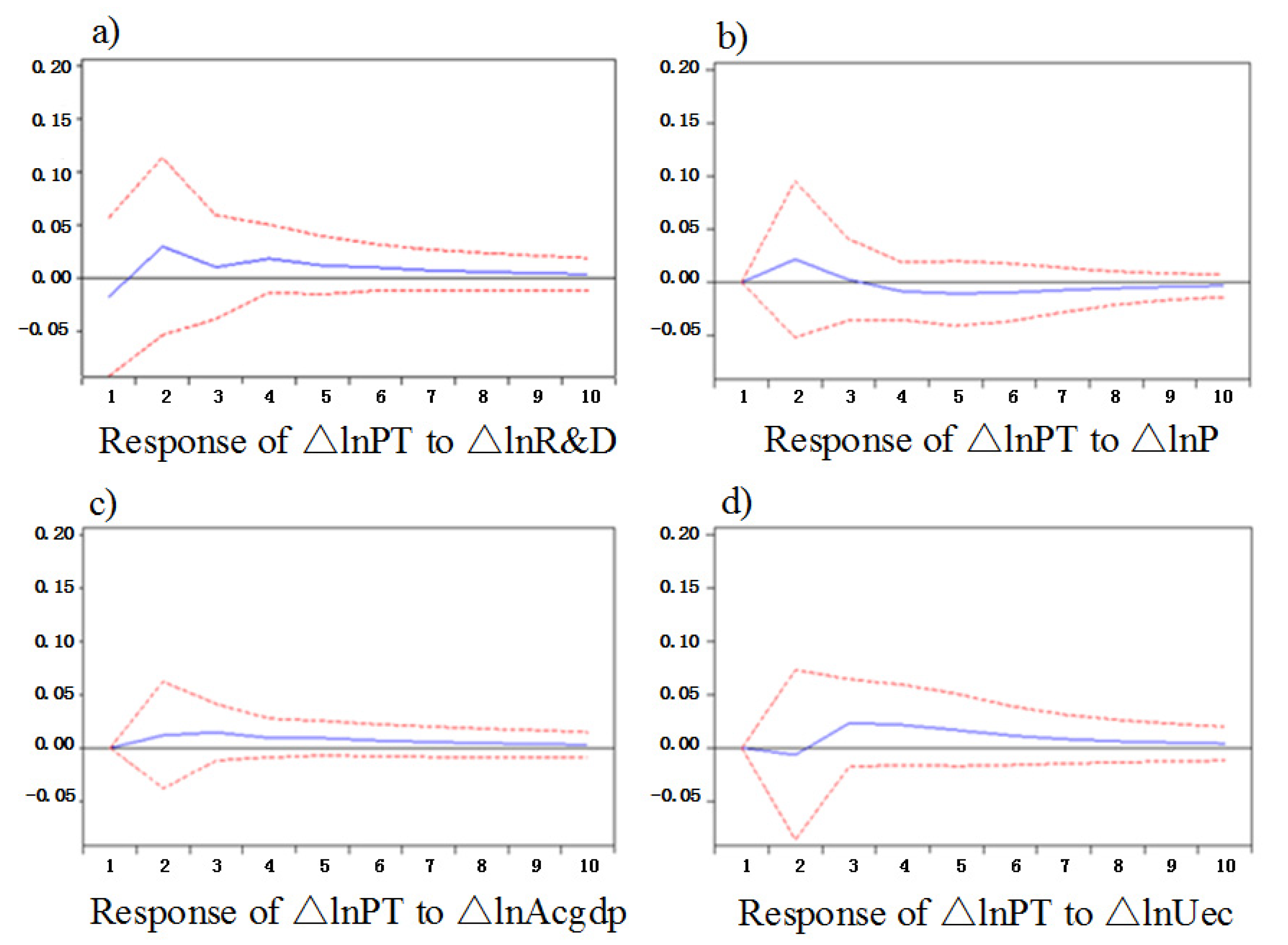
Since each series passes the stationarity test after checking the scores, the VAR model fits well and the corresponding VAR model is equally stable, satisfying the impulse response function assumption condition. Therefore, it is possible to analyze the impact of dynamic shocks on the whole system when one error term is changed. Figure 2 shows the impulse response function curve, the horizontal axis is the tracking period of the response function and the vertical axis is the response of each indicator to the GTIB of construction enterprises. The solid line is the calculated value of the response function, and the dashed line is the confidence interval of the response value ± two standard deviations. In this paper, the tracking period of the response function is set to 10, and the impulse function plot of each indicator against the level of GTIB of construction enterprises is calculated by combining software (Figure 2).

In Figure 2, the graphs of impulse response functions of the impact of the level of the GTIB of construction enterprises are included for four indicators. The shocks of these four variables have different degrees of influence on the level of the GTIB of construction enterprises. Among them, Figure 2a shows that the impact of the shocks of R&D on the level of the GTIB of construction enterprises’ development starts to gradually increase from a negative impact to a positive impact in period 1, fluctuates after reaching the peak in period 2 and reaches the peak for the second time in period 4, after which the degree of impact gradually converges to smoothness over time. Figure 2b shows that the positive impact of the shocks of P on the level of the GTIB of construction enterprises starts to decrease after reaching its peak in period 2. The positive effect of the shock of P on the level of the GTIB of construction enterprises starts to decrease after reaching its peak in period 2, and then decreases and becomes negative in period 3 and finally gradually converges to a stable level. Figure 2c shows that the effect of the shock of Uec on the level of GTIB of construction enterprises starts to be negative, gradually increases to a positive effect in period 2, reaches its peak in period 3 and then gradually converges to a stable level. Figure 2d shows that the effect of the shock of Acgdp on the level of the GTIB of construction enterprises is positive and has a low impact effect. It can be seen that R&D has a unidirectional positive effect on the level of the GTIB of construction enterprises; P indicators have a positive and negative alternating effect on the level of the GTIB of construction enterprises; Acgdp has a small effect on the level of the GTIB of construction enterprises.

4.6. Analysis of Variance Decomposition

In this paper, based on the VAR model, each time series is subjected to a heteroskedasticity test, a time series smoothness test and an impulse response function analysis. The variance decomposition analysis is performed on each series to further test the relative importance of each dependent variable on the GTIB of construction enterprises. Variance decomposition is the decomposition of the mean squared deviation of an endogenous variable into the proportional contribution of shocks to all variables to understand the degree of influence of these variables. The results of the analysis are shown in

Table 9. Variance Decomposition of DLNPT.

Period	S.E.	ΔlnPT	ΔlnR&D	ΔlnAcgdp	ΔlnP	ΔlnUec
1	0.16	100.00	0.00	0.00	0.00	0.00
2	0.19	94.01	3.44	0.06	2.32	0.18
3	0.20	91.04	3.61	0.76	2.43	2.13
4	0.20	88.14	4.50	1.26	2.41	3.69
5	0.21	86.36	4.80	1.78	2.51	4.55
6	0.21	85.29	5.04	2.11	2.63	4.94
7	0.21	84.69	5.17	2.32	2.69	5.12
8	0.21	84.34	5.26	2.45	2.72	5.23
9	0.21	84.12	5.32	2.53	2.73	5.29
10	0.21	83.97	5.36	2.59	2.74	5.34

.

As can be seen from the table, the greatest degree of influence on the GTIB of construction enterprises is the R&D indicator. The contribution rate in the second cycle is 3.44%, which gradually increases in the following cycles and reaches 5.36%, with a general trend of gradual increase. The second degree of influence is Uec, which grows rapidly in the first three cycles and reaches 2.16%, and then the degree of influence increases year by year and reaches 5.34% in the tenth period. The degree of influence of Acgdp and P on the development level of the GTIB of construction enterprises is not very different. The degree of influence of Acgdp starts to increase rapidly from 0.06% to 2.59% in cycles 3–6, while the degree of influence of P indicator increases relatively steadily, only by 0.42% in 10 cycles.

4.7. Granger Causality Analysis

According to the theory of Granger causality analysis mentioned in the previous section, Granger causality analysis is performed for each group of series that passed the smoothness test. The lag order chosen is the optimal lag order identified in the previous section, and the test results are as follows in

Table 10. Pairwise Granger Causality Tests.

Null Hypothesis:	Obs	F-Statistic	Prob.	Result
lnAcgdp does not Granger Cause lnPT	18	19.90	0.00	Yes
lnPT does not Granger Cause lnAcgdp		14.01	0.00	Yes
lnR&D does not Granger Cause lnPT	18	17.43	0.00	Yes
lnPT does not Granger Cause lnR&D		5.57	0.03	Yes
lnP does not Granger Cause lnPT	18	11.90	0.00	Yes
lnPT does not Granger Cause lnP		1.98	0.18	No
lnUec does not Granger Cause lnPT	18	9.30	0.01	Yes
lnPT does not Granger Cause lnUec		0.27	0.61	No

.

From Table 10, it is clear that Acgdp and R&D are Granger causes of PT with each other. This indicates that the rate of development of the construction industry and R&D investment in science and technology and the level of GTIB of construction enterprises influence each other and respond to each other’s development. p and Uec are the Granger cause of PT. This indicates that environmental regulation and investment in urban environmental infrastructure can influence the level of the GTIB of construction enterprises, and the level of the GTIB of construction enterprises can also reflect the status of environmental regulation and investment in urban environmental infrastructure. This paper also used a multivariate Johansen cointegration test to test the cointegration relationship among the indicators, and the results showed that there were four cointegration relationships between Uec, R&D, P, Acgdp and PT.

5. Discussion

This paper finds that R&D indicators, as well as Uec indicators, show a unidirectional positive effect on the level of the GTIB of construction enterprises and the greatest degree of influence. This paper concludes that direct economic investment by the government has a catalytic effect on the level of construction enterprises, that the effect is greater at the beginning of the effect and that it plateaus over time. This is consistent with the findings of Zhou that government incentives are not effective in promoting the GTIB of construction enterprises because of the complexity of the procedures, but that direct incentives are more important [48]. At the same time, improving the level of green development of enterprises cannot be separated from the efforts of the government [49].Therefore, H1 passes the test.

The impact of Acgdp on the level of the GTIB of construction enterprises has been positively influenced, with a small degree of influence but a rapid increase in the initial degree of influence, followed by a gradual stabilization of the degree of influence. This paper concludes that the development of the construction industry has a facilitating effect on the level of the GTIB of construction enterprises, especially at the stage of rapid development of the industry, where the facilitating effect is more significant. However, as the development rate slows down, the promotion effect gradually remains stable. This is in line with the findings of Ozorhon and Oral [50], who found that the factors related to enterprises in the industry have a facilitating effect on green innovation in the industry. Moreover, this paper uses the Johansen co-integration test to test the co-integration relationship between the dependent and independent variables. Therefore, H2 passes the test.

In contrast, the impact of environmental regulations on the GTIB of construction enterprises is not linear, and the degree of impact is small and does not change much over time. This paper suggests that the reason for this phenomenon is that, as the level of GTIB of construction enterprises in China improves and the green development of the construction industry becomes more mature, the number of related policies decreases. This is consistent with the findings of several scholars. Among them, Yang et al. obtained a similar conclusion through evolutionary game analysis that positive policy incentives have negative effects [51]. Zhang et al. pointed out that, similar to the results of this paper, the Chinese government has launched a variety of policies to encourage the practice of green buildings, but that green certified buildings account for only a small proportion of China’s booming real estate market and are unevenly distributed across its regions [52].Therefore, H3 passes the test.

At the same time, the Granger causality test results show that Acgdp, R&D and PT are Granger causes for each other, and that P and Uec are Granger causes for PT. To sum up, it is considered that there is a long-term equilibrium relationship between Acgdp, R&D, Uec, P and PT, which will affect the level of GTIB in the construction industry. The research results of this paper are consistent with the research results of Guo et al., who believed that environmental regulations, direct investment and regional level development will have an impact on green technology innovation [53].

6. Conclusions and Policy Implications

To explain the mechanism of action that affects the GTIB of construction enterprises, this paper constructs a model of the GTIB of construction enterprises based on a multiple linear regression method and conducts impulse response function analysis, variance decomposition analysis, co-integration test and Granger causality analysis. The main findings are as follows:

• The influence of Uec and R&D on the GTIB of construction enterprises is large and remains significantly positive, reflecting that direct economic investment by the government can better promote the level of GTIB of construction enterprises.
• The influence of Acgdp on the GTIB of construction enterprises grows faster at the beginning and remains stable over time, indicating that the development speed of the construction industry has a positive influence on the level of the GTIB of construction enterprises.
• The degree of influence of P on the GTIB of construction enterprises is positive at the beginning, but gradually shows negative influence over time, which confirms that environmental regulation has a facilitating effect on the GTIB of construction enterprises at the beginning and then shows a hindering effect at the middle and later stages.

The findings of this paper have important theoretical and practical significance:

• The findings of this paper theoretically enrich the relevant research on the role mechanisms affecting the GTIB of construction enterprises by constructing a new model of the GTIB of construction enterprises, by introducing a VAR model and by clarifying the role mechanism affecting the GTIB of construction enterprises in China through four kinds of analysis. Therefore, this paper can provide a feasible solution for the improvement of GTIB construction enterprises around the world.
• Given the late start of green building in China, there is a relative lack of in-depth research on the GTIB of construction enterprises in China. Therefore, this paper analyzes from the perspective of urban construction development as well as industry to broaden the research framework of the GTIB of construction enterprises and provide evidence from China for the field.
• The existing econometrics in construction enterprises is mostly applied to research on environmental protection, pollution analysis and development trend prediction of construction enterprises. Therefore, this paper provides new ideas for the study of the GTIB of construction enterprise in the world.

The conclusion of this paper not only enriches the theoretical research related to the role mechanism of the GTIB of construction enterprises, but also has some implications for government policies and construction enterprise managers in formulating strategic plans about green development in management practice. Meanwhile, countries around the world can refer to the conclusions in this paper. It improves the level of GTIB of their construction enterprise according to their own national conditions.

• When the government or enterprise managers make decisions to improve the level of the GTIB of construction enterprises, they can do so by increasing direct investment in order to enhance the level of the GTIB of construction enterprises.
• The increase in the development rate of the construction industry also has a catalytic effect on the GTIB of construction enterprises, but its degree of influence only grows faster at the beginning of the effect and the degree of influence gradually plateaus over time. Therefore, maintaining a steady growth of the construction industry is the most effective way to improve the level of the GTIB of construction enterprises.
• Then, the government’s environmental regulations and the quantity of these regulations can be kept correspondingly stable as the government gradually improves the policies related to the green development of the construction industry, i.e., the government can change from increasing the quantity of environmental regulations to improving the content and quality of environmental regulations. When formulating environmental regulations, countries should fully consider the characteristics of their construction enterprises. This will facilitate the development of the GTIB of construction enterprises.

As with most studies, there are some limitations to this paper’s research. In data selection, only time series data from 2000 to 2018 were selected in this paper because the government has not yet provided the complete data for the last two years. Moreover, there are many factors that affect the level of the GTIB of construction enterprises, e.g., market maturity and construction enterprises’ willingness for GTIB. This paper has not yet examined the above-mentioned factors that are difficult to quantify, which also provides an opportunity for researchers to further validate the mechanism of these factors on the GTIB of construction enterprises in the future using computer simulation and other means.

References

- Meng, J.; Liu, J.; Xu, Y.; Guan, D.; Liu, Z.; Huang, Y.; Tao, S. Globalization and pollution: Tele-connecting local primary PM2.5 emissions to global consumption. Proc. R. Soc. A Math. Phys. Eng. Sci. 2016, 472, 20160380. [Google Scholar] [CrossRef] [PubMed] [Green Version]
- Zhang, L.; Liu, B.; Du, J.; Liu, C.; Wang, S. CO2 emission linkage analysis in global construction sectors: Alarming trends from 1995 to 2009 and possible repercussions. J. Clean. Prod. 2019, 221, 863–877. [Google Scholar] [CrossRef]
- Hong, J.; Shen, Q.; Xue, F. A multi-regional structural path analysis of the energy supply chain in China’s construction industry. Energy Policy 2016, 92, 56–68. [Google Scholar] [CrossRef] [Green Version]
- La-Rosa, D.; Privitera, R.; Barbarossa, L.; La-Greca, P. Assessing spatial benefits of urban regeneration programs in a highly vulnerable urban context: A case study in Catania, Italy. Landsc. Urban Plan. 2017, 157, 180–192. [Google Scholar] [CrossRef]
- Patent Search and Analysis. Available online: http://pss-system.cnipa.gov.cn/sipopublicsearch/patentsearch/tableSearch-showTableSearchIndex.shtml (accessed on 1 November 2021).
- National Bureau of Statistics. China Statistical Yearbook 2020; China Statistics Press: Beijing, China, 2020.
- Zhang, Y.; Kang, J.; Jin, H. A review of green building development in China from the perspective of energy saving. Energies 2018, 11, 334. [Google Scholar] [CrossRef] [Green Version]
- Li, X.; Du, J.; Long, H. Theoretical framework and formation mechanism of the green development system model in China. Environ. Dev. 2019, 32, 100465. [Google Scholar] [CrossRef]
- Li, X.; Du, J.; Long, H. Understanding the green development behavior and performance of industrial enterprises (GDBP-IE): Scale development and validation. Int. J. Environ. Res. Public Health 2020, 17, 1716. [Google Scholar] [CrossRef] [Green Version]
- Long, H.; Liu, H.; Li, X.; Chen, L. An evolutionary game theory study for construction and demolition waste recycling considering green development performance under the Chinese government’s reward–penalty mechanism. Int. J. Environ. Res. Public Health 2020, 17, 6303. [Google Scholar] [CrossRef]
- Liu, H.; Long, H.; Li, X. Identification of critical factors in construction and demolition waste recycling by the grey-DEMATEL approach: A Chinese perspective. Environ. Sci. Pollut. Res. 2020, 27, 8507–8525. [Google Scholar] [CrossRef]
- Li, X.; Huang, R.; Dai, J.; Shen, Q. Research on the evolutionary game of construction and demolition waste (CDW) recycling units’ green behavior, considering remanufacturing capability. Int. J. Environ. Res. Public Health 2021, 18, 9268. [Google Scholar] [CrossRef]
- Cull, R.; Li, W.; Sun, B.; Xu, L.C. Government connections and financial constraints: Evidence from a large representative sample of Chinese firms. J. Corp. Financ. 2015, 32, 271–294. [Google Scholar] [CrossRef] [Green Version]
- Chang, R.; Soebarto, V.; Zhao, Z.; Zillante, G. Facilitating the transition to sustainable construction: China’s policies. J. Clean. Prod. 2016, 131, 534–544. [Google Scholar] [CrossRef]
- Darnall, N.; Henriques, I.; Sadorsky, P. Adopting proactive environmental strategy: The influence of stakeholders and firm size. J. Manag. Stud. 2010, 47, 1072–1094. [Google Scholar] [CrossRef]
- Chen, L.; Gao, X.; Hua, C.; Gong, S.; Yue, A. Evolutionary process of promoting green building technologies adoption in China: A perspective of government. J. Clean. Prod. 2021, 279, 123607. [Google Scholar] [CrossRef]
- Darko, A.; Chan, A.P.C.; Yang, Y.; Ming, S.; He, B.J. Influences of barriers, drivers, and promotion strategies on green building technologies adoption in developing countries: The Ghanaian case. J. Clean. Prod. 2018, 200, 687–703. [Google Scholar] [CrossRef]
- Bas Cerdá, M.D.C.; Ortiz Moragón, J.; Ballesteros Pascual, L.; Martorell Alsina, S.S. Evaluation of a multiple linear regression model and SARIMA model in forecasting 7Be air concentrations. Chemosphere 2017, 177, 326–333. [Google Scholar] [CrossRef]
- Sims, C.A. Macroeconomics and reality. Econom. J. Econom. Soc. 1980, 48, 1–48. [Google Scholar] [CrossRef] [Green Version]
- Hao, Y.; Zhu, L.; Ye, M. The dynamic relationship between energy consumption, investment and economic growth in China’s rural area: New evidence based on provincial panel data. Energy 2018, 154, 374–382. [Google Scholar] [CrossRef]
- Davidson, R.; MacKinnon, J.G. Estimation and Inference in Econometrics; OUP Catalogue: Oxford, UK, 1993. [Google Scholar]
- Olson, E.; Vivian, A.J.; Wohar, M.E. The relationship between energy and equity markets: Evidence from volatility impulse response functions. Energy Econ. 2014, 43, 297–305. [Google Scholar] [CrossRef] [Green Version]
- Fang, S.; Jia, R.; Tu, W.; Sun, Z. Research on the influencing factors of comprehensive water consumption by impulse response function analysis. Water 2017, 9, 18. [Google Scholar] [CrossRef] [Green Version]
- Kim, K.Y.; Patel, P.C. Employee ownership and firm performance: A variance decomposition analysis of European firms. J. Bus. Res. 2017, 70, 248–254. [Google Scholar] [CrossRef] [Green Version]
- Borozan, D. Exploring the relationship between energy consumption and GDP: Evidence from Croatia. Energy Policy 2013, 59, 373–381. [Google Scholar] [CrossRef]
- You, J. China’s energy consumption and sustainable development: Comparative evidence from GDP and genuine savings. Renew. Sustain. Energy Rev. 2011, 15, 2984–2989. [Google Scholar] [CrossRef]
- Granger, C.W.J. Investigating causal relations by econometric models and cross-spectral methods. Econom. J. Econom. Soc. 1969, 37, 424–438. [Google Scholar] [CrossRef]
- Bakirtas, T.; Akpolat, A.G. The relationship between energy consumption, urbanization, and economic growth in new emerging-market countries. Energy 2018, 147, 110–121. [Google Scholar] [CrossRef]
- Zhang, Y. Dynamic effect analysis of meteorological conditions on air pollution: A case study from Beijing. Sci. Total Environ. 2019, 684, 178–185. [Google Scholar] [CrossRef] [PubMed]
- Kong, F.; He, L. Impacts of supply-sided and demand-sided policies on innovation in green building technologies: A case study of China. J. Clean. Prod. 2021, 294, 126279. [Google Scholar] [CrossRef]
- Wang, B.; Zhao, C. China’s Green Technological Innovation—Patent Statistics and Influencing Factors. J. Ind. Technol. Econ. 2019, 38, 53–66. (In Chinese) [Google Scholar]
- Zhang, R.; Sun, K.; Delgado, M.S.; Kumbhakar, S.C. Productivity in China’s high technology industry: Regional heterogeneity and R&D. Technol. Forecast. Soc. Chang. 2012, 79, 127–141. [Google Scholar] [CrossRef] [Green Version]
- Chen, H.; Lin, H.; Zou, W. Research on the regional differences and influencing factors of the innovation efficiency of China’s high-tech industries: Based on a shared inputs two-stage network DEA. Sustainability 2020, 12, 3284. [Google Scholar] [CrossRef] [Green Version]
- Yin, S.; Zhang, N.; Li, B. Enhancing the competitiveness of multi-agent cooperation for green manufacturing in China: An empirical study of the measure of green technology innovation capabilities and their influencing factors. Sustain. Prod. Consum. 2020, 23, 63–76. [Google Scholar] [CrossRef]
- Peng, W.; Wen, Z.; Kuang, C. The Spatial Pattern and Influencing Factors of Green Innovation. J. Guangdong Univ. Financ. Econ. 2019, 34, 25–37. (In Chinese) [Google Scholar]
- Zhang, H.; Shi, L. Human Capital and Regional Innovation: An Empirical Study Based on Spatial Dubin Model. J. Hunan Univ. Soc. Sci. 2018, 32, 49–57. [Google Scholar] [CrossRef]
- Sun, Y.; Mei, X.; Chen, S. Study on the temporal and spatial pattern and driving factors of green technology innovation in urban agglomeration of Yangtze River Delta. Jiang-Huai Trib. 2021, 13–22+61. Available online: http://www.jhlt.net.cn/CN/article/downloadArticleFile.do?attachType=PDF&id=11878 (accessed on 1 November 2021).
- Hu, W.F.; Kong, D.L.; He, X.H. Analysis on influencing factors of green building development based on BP-WINGS. Soft Sci. 2020, 75–81. [Google Scholar] [CrossRef]
- Hui, N.; Ge, P. The Correlation between Industrial Scale, R&D Investment and the Development of Software Industry. Reform 2015, 31, 100–109. Available online: http://www.refo.cbpt.cnki.net/WKE/WebPublication/kbDownload.aspx?fn=REFO201506013 (accessed on 1 November 2021).
- Yang, J.Y.; Chen, W. Research on the evaluation model of the modernization level of urban construction in Jiangsu Province, China. Sci. China Technol. Sci. 2010, 53, 2510–2514. [Google Scholar] [CrossRef]
- Hwang, B.G.; Zhu, L.; Tan, J.S.H. Green business park project management: Barriers and solutions for sustainable development. J. Clean. Prod. 2017, 15, 209–219. [Google Scholar] [CrossRef]
- Hart, S.L.; Dowell, G. Invited editorial: A natural-resource-based view of the firm: Fifteen years after. J. Manag. 2011, 37, 1464–1479. [Google Scholar] [CrossRef]
- Zhang, F.; Wang, Y.; Ma, X.; Wang, Y.; Yang, G.; Zhu, L. Evaluation of resources and environmental carrying capacity of 36 large cities in China based on a support-pressure coupling mechanism. Sci. Total Environ. 2019, 688, 838–854. [Google Scholar] [CrossRef]
- Yao, L.; Liu, C.; Mao, Y. The latest comparison of China’s comprehensive power with that of seven Western countries. Stat. Res. 2000, 3–8. [Google Scholar] [CrossRef]
- Qiluan, Z.; Weiqiang, Z.; Ling, L. Research on the Inner Relationship between Chinese Economic Growth and Energy Consumption—Based on Granger Causality Test of the VECM Model and Grey Relevance Analysis. Contemp. Econ. Manag. 2014, 36, 30–34. [Google Scholar] [CrossRef]
- Zhong, W. Mineral rights agglomeration, economic growth & regional poverty alleviation. China Popul. Resour. Environ. 2017, 27, 117–125. Available online: http://www.cpre.sdnu.edu.cn/WKC/WebPublication/kbDownload.aspx?fn=ZGRZ201702017 (accessed on 1 November 2021).
- Li, Y.; Shen, J.; Xia, C.; Xiang, M.; Cao, Y.; Yang, J. The impact of urban scale on carbon metabolism—A case study of Hangzhou, China. J. Clean. Prod. 2021, 292, 126055. [Google Scholar] [CrossRef]
- Zhou, Y. State power and environmental initiatives in China: Analyzing China’s green building program through an ecological modernization perspective. Geoforum 2015, 61, 1–12. [Google Scholar] [CrossRef] [Green Version]
- Li, X.; Dai, J.; Li, J.; He, J.; Liu, X.; Huang, Y.; Shen, Q. Research on the Impact of Enterprise Green Development Behavior: A Meta-Analytic Approach. Behav. Sci. 2022, 12, 35. [Google Scholar] [CrossRef]
- Ozorhon, B.; Oral, K. Drivers of innovation in construction projects. J. Constr. Eng. Manag. 2017, 143, 04016118. [Google Scholar] [CrossRef]
- Yang, X.; Zhang, J.; Shen, G.Q.; Yan, Y. Incentives for green retrofits: An evolutionary game analysis on Public-Private-Partnership reconstruction of buildings. J. Clean. Prod. 2019, 232, 1076–1092. [Google Scholar] [CrossRef]
- Zhang, L.; Wu, J.; Liu, H. Turning green into gold: A review on the economics of green buildings. J. Clean. Prod. 2018, 172, 2234–2245. [Google Scholar] [CrossRef]
- Guo, Y.; Xia, X.; Zhang, S.; Zhang, D. Environmental regulation, government R&D funding and green technology innovation: Evidence from China provincial data. Sustainability 2018, 10, 940. [Google Scholar] [CrossRef] [Green Version]