Article

Off-Site Construction Three-Echelon Supply Chain Management with Stochastic Constraints: A Modelling Approach

1
School of Industrial and Systems Engineering, College of Engineering, University of Tehran, Tehran 1439955961, Iran
2
School of Industrial Engineering, K. N. Toosi University of Technology (KNTU), Tehran 1999143344, Iran
3
Department of Management, Alborz Campus, University of Tehran, Tehran 1417733631, Iran
4
School of Built Environment, University of New South Wales, Sydney 2052, Australia
*
Author to whom correspondence should be addressed.
Buildings 2022, 12(2), 119; https://doi.org/10.3390/buildings12020119
Submission received: 31 December 2021 / Revised: 19 January 2022 / Accepted: 21 January 2022 / Published: 25 January 2022
(This article belongs to the Special Issue Construction Management and Disaster Risk Management)

Abstract

:
Off-site construction is becoming more popular as more companies recognise the benefits of shifting the construction process away from the construction site and into a controlled manufacturing environment. However, challenges associated with the component supply chain have not been fully addressed. As a result, this study proposes a model for three-echelon supply chain supply management in off-site construction with stochastic constraints. In this paper, multiple off-site factories produce various types of components and ship them to supplier warehouses to meet the needs of the construction sites. Each construction site is directly served by a supplier warehouse. The service level for each supplier warehouse is assumed to be different based on regional conditions. Because of the unpredictable nature of construction projects, demand at each construction site is stochastic, so each supplier warehouse should stock a certain number of components. The inventory control policy is reviewed regularly and is in (R, s, S) form. Two objectives are considered: minimising total cost while achieving the desired delivery time for construction sites due to their demands and balancing driver workloads during the routeing stage. A grasshopper optimisation algorithm (GOA) and an exact method are used to solve this NP-hard problem. The findings of this study contribute new theoretical and practical insights to a growing body of knowledge about supply chain management strategies in off-site construction and have implications for project planners and suppliers, policymakers, and managers, particularly in companies where an unplanned supply chain exacerbates project delays and overrun costs.

1. Introduction

Due to globalisation and industrialisation, environmental concerns are increasing, putting natural resources at risk [1]. These issues have been heavily influenced by the construction industry [2]. The increased construction activities have many negative consequences, including the depletion of natural resources and waste generation, energy consumption, greenhouse gas emissions, and risks to public safety [3,4]. The construction industry is the primary source of glasshouse gas (GHG) emissions and a major consumer of global energy [5,6]. In the absence of innovative techniques and technologies applied in the construction industry, this industry’s adverse impacts would exacerbate even more [7]. Current construction methods are not well suited to meet the rising demand for rapid construction [8,9]. Construction activities should be more efficient in meeting sustainability goals [10]. Some construction activities could see productivity increases of five to ten times their current level if moved to an off-site construction system [11]. As a result, considerable attention should be devoted to implementing off-site construction approaches in the construction industry to increase its efficiency and productivity [12].
In off-site construction methods, building components are manufactured in a workshop or a factory and then transported to the construction sites or supplier warehouses, where they are assembled [13]. This allows for better coordination between skilled labourers and automated equipment employed in off-site construction projects [14]. Furthermore, implementing this construction approach in the construction industry can improve the quality, and the number of building defects is reduced due to better monitoring [15]. Off-site construction methods are more environmentally friendly and safer than conventional construction techniques [16].
While the advantages of off-site construction methods are increasingly documented [17], they are currently associated with some challenges, particularly in material procurement [18]. The problem of ensuring component availability for project activities while simultaneously minimising unnecessary inventory in the off-site construction system remains unresolved. Each component in off-site construction projects has a specific purpose. To have a successful project, all components should be available when needed [11]. Therefore, supply chain strategies should be incorporated and explored in this construction system to mitigate the risks associated with the on-time procurement of components for construction sites [18].
Material procurement in this system is a multi-echelon supply chain starting from preparing detailed design and shop drawings for structure components manufactured in a factory or workshop [18]. Following that, these components are warehoused and shipped to construction sites where they should be installed. These components are tailored to the specifications of each project. As a result, prefabricators are unable to manufacture these components prior to receipt of orders [18]. Additionally, due to the weight and bulk of these components, contractors are unable to maintain large buffer stocks in anticipation of delivery delays [18,19]. Any unplanned action in the supply chain of components at the procurement strategies has a ripple effect on the subsequent stages, resulting in an inefficient off-site construction. As a result, more modelling techniques are required to implement supply chain models and techniques in off-site construction.
To address current gaps in this research area, this study considers a transportation–location–inventory–routing problem that simultaneously covers the different dimensions of the distribution network in the supply chain of off-site construction methods as supposing multiple suppliers that send various components to different supplier warehouses. Further, due to the location conditions of each warehouse, a certain service level for each supplier warehouse is considered and owing to the various types of construction components, as well as storage limitations, a risk level of exceeding maximum inventory for each component is considered. In addition, some off-site factories provide a shorter delivery time for their strategic construction projects, the demands of which are higher than others. Therefore, a constraint is applied to the model to ensure that the weighted average construction project lead time is acceptable. The routing problem has been addressed in off-site construction methods, such as [20]; however, the ordering system in the warehouse is neglected, and the demand was deterministic, while the uncertainty in the demands of construction projects and considering safety stock in the supplier warehouses make the model of this study closer to the actual state. In this regard, we consider the (R, s, S) ordering policy, which is one of the ordering systems to determine the inventory level of supplier warehouses and applies when continuous inventory checking is not possible. Considering all these aspects makes the study more appropriate for the real off-site construction methods than previous studies.
As the substantial contributions of the present study, a mixed-integer bi-objective mathematical model is proposed to develop a transportation–location–inventory–routing Problem. Moreover, multiple suppliers, which send various components to supplier warehouses to satisfy construction projects’ demand, have been considered. This study aims to minimise the total cost of the distribution network and achieve the desired delivery time for construction sites due to their demands. To solve the proposed bi-objective supply chain model and in order to generate a properly balanced set of routes at minimum cost, an equilibrium objective function has been applied by converting two objective functions into one. Furthermore, the transportation–location–inventory–routing problem belongs to the class of NP-hard problems; therefore, it needs a meta-heuristic method to solve the problem at a large size, and for small size problems, we use the exact method.
The rest of this study is structured as follows. Related studies are presented in Section 2. The problem statement and the proposed mathematical model are provided briefly in Section 3. Section 4 then describes the proposed approach to solve the problem in detail. Section 5 presents the computational tests and analysis. Section 6 presents a comprehensive sensitivity analysis. Section 7 provides discussion and managerial insights based on the study’s findings. Finally, the conclusion and directions for future studies are presented in Section 8.

2. Related Works

2.1. Off-Site Construction

Hussein, Eltoukhy, Karam, Shaban, and Zayed [18] recently presented a comprehensive review of off-site construction supply chain management models. This research area has received increased attention in recent years. Jeong et al. [21] used a simulation approach to determine the supply chain’s CO2 emissions, productivity, and cost. Zhai et al. [22] presented a coordination scheme for the contractor and the prefabricator to achieve a win-win coordination scheme. Zhai et al. [23] created a system to balance the contractor and the transporter. Kong et al. [24] presented an approach that employs the idea of Just in Time to the supply chain by taking two major factors into account, including on-site assembly time and transportation time. The proposed model minimises total penalty costs by presenting a polynomial-time algorithm. The model’s flaw was that transportation times are calculated based on limited traffic levels and homogeneous vehicle types, limiting the model’s applicability in real-world scenarios. Wang et al. [25] used GA to develop a simulation-optimisation model to reach a near-optimal PC production sequence. They then used a DES model to investigate the effects of the achieved production sequence on the logistics stages’ performance without considering the on-site installation stage. Lee and Hyun [26] used GA to combine a MiC supply chain simulation model. The model was used to determine an on-site installation schedule, the number of transportation trucks, and a near-optimal production sequence, for MiC modules to reduce the number of modules stacked on-site. Bamana et al. [27] provided a simulation model to assess the practical impact of the Just in Time and lean principles on construction project completion time and labour utilisation. Even though the suggested model was practical, it was limited to medium-sized wooden construction sites. Hsu et al. [28] created a robust optimisation model for determining the best production and logistics decisions that improve economic sustainability by lowering supply chain expenses. Chen et al. [29] suggested both static and dynamic collaborative scheduling mechanisms. The static one tries near-optimal time and resource schedules to minimise total production and construction costs, whereas the dynamic one tries to minimise total costs incurred due to rescheduling in the event of supply chain disruptions. The simulated annealing algorithm was used to solve the optimisation problem. Yi et al. [30] formulated a model to decide the capacity of each truck employed to transfer panels from the manufacturing site to the installation location. The model was created to reduce total costs, involving holding costs and transportation. A greedy algorithm was used to obtain the solution. However, the model only takes into account the product’s weight while ignoring the product’s 3D volumetric features. This could limit the number of products carried, resulting in inefficient truck utilisation. Lyu et al. [31] created a simulation model to suggest the concept of zero-warehousing smart manufacturing, which entailed eliminating all non-value-added operations. The concept’s effectiveness was demonstrated in a case study in Hong Kong. Liu et al. [32] formulated a multi-integer linear programming model for determining the best precast construction storage plan. The model reduced relocation times, as well as outbound and inbound transportation expenses. Multiple stakeholders should be able to benefit from a win-win situation in the collaborative supply chain problem. Ahn et al. [33] concentrated on improving transportation cost estimation, which was previously calculated using a fixed cost approach. They used GIS techniques to collect routing information. The extracted data was fed into a support vector regression model, which predicted transportation costs. Lee et al. [34] presented a heuristic method for finding the near-optimal staking plans for exterior wall panels on A-frame trailers. The method reduces the number of trailer trips required while minimising double-handling and guaranteeing the stability of transported panels. Hussein, Eltoukhy, Darko, and Eltawil [17] proposed a simulation-optimisation approach for the planning of off-site construction projects and conducted a comparative study of recent swarm intelligence meta-heuristics, including the firefly algorithm, grey wolf optimisation, the whale optimisation algorithm, the salp swarm algorithm, and one improved version of the well-known bat algorithm. Yazdani, Kabirifar, Fathollahi-Fard, and Mojtahedi [11] explored production scheduling of off-site prefabricated construction components considering sequence-dependent due dates. Three integrated simulation-optimisation algorithms were proposed to address the uncertainties and complexities associated with the stochastic nature of production problems. MacAskill et al. [35] explored how OSC techniques that reduce development timeframes may better deliver demography-linked housing supply to vulnerable groups waiting for affordable rental housing. Yang et al. [36] identified and categorised sources of uncertainties (SoUs) affecting off-site logistics in the context of modular high-rise building projects in high-density cities. Liu et al. [37] employed the scientometric method to analyse the literature on prefabricated buildings in the past ten years through analysis of co-authors, co-words, and co-citation. Nguyen et al. [38] analysed the literature on stakeholder relationships towards identifying patterns of relationships within the off-site construction context. Recently, Masood et al. [39] conducted a systematic review of the available literature on supply chain management within prefabricated house-building research.

2.2. Supply Chain Modelling

In the supply chain management research area, there are some relevant studies. Guimarães et al. [40] addressed a multi-supplier inventory–routing problem (IRP) with capacitated customer points and vehicles. In order to manage the orders, Yao et al. [41] proposed a multi-supplier and multi-product location inventory problem, which was based on periodic inventory control policy (R, T) with the aim of determining the inventory level of each distribution centre. Cabrera et al. [42] analysed the effects of inventory policies on the decisions about distributing the products. To do this, a single-supplier and multi-product inventory location model with stochastic constraints has been represented, which was based on a periodic inventory control policy (R, s, S). Subsequently, Amiri-Aref et al. [43] presented a multi-period location–inventory problem (LIP) to place the potential DCs, as well as determining the inventory reorder point level in each period based on (s, S) policy.
Indeed, different real-world issues have made supply chain management more complex to make accurate decisions. Due to the traffic conditions, some supplier warehouses have been constructed on the outskirts of cities to store goods as intermediate points because plants cannot deliver goods directly to customers. Hence, the optimum location of supplier warehouses to be established can be one of the critical decisions that location problems cope with it [44]. Since inventory costs include ordering costs, inventory storage outlays during each period, as well as lost costs due to the shortages, retailers, and middle warehouses are always concerned about the amount of ordering and safety stock in stores in the way to reduce total costs while concomitantly achieving maximum customer satisfaction [45]. Therefore, due to the necessity of simultaneously considering various dimensions of the distribution system, several cases have been investigated LIP in which the decision-maker can ascertain both locations of depots, such as warehouses, and the number of inventory variables. In this field, the LIP model proposed by Daskin et al. [46], contrary to an incapacitated facility location problem, the high local delivery costs may balance by decreasing safety stock and working inventory. Furthermore, LIP has been modified by Shen et al. [47], considering risk-pooling in that some retailers can be substituted for DCs to serve other retailers.
One of the most significant elements of a supply chain of an off-site construction system is the transportation mode. Various types of vehicles with different capacities affect freight costs and help managers make more appropriate decisions according to the lead times and the types of available vehicles [48,49]. Moreover, a network of roads enables interconnection between different locations, so choosing the most suitable route according to the arrival time is considered fundamental to the practice. In this regard, the integration of inventory and transportation decisions, which optimises the ordering and delivery policies, was represented by Zhao et al. [50]. The first research, which focused on a transportation–location–routing problem, was investigated by Martínez-Salazar et al. [51]. This paper integrated decisions about the number of vehicles with limited capacity with the location routing problem. Furthermore, there are studies about transportation–inventory problems (TIP) [52]. For instance, Lee et al. [53] developed a TIP model, and unlike traditional models, the number of buyers and the number of intermediate stops may change in each period.
Moreover, many authors have taken into account the IRP [54,55]. Fokkema et al. [56] proposed a continuous supply-centric IRP for the first time, in which inventories are stored in containers that can be both movable and stable storages of capacitated vehicles and depots, respectively. Further, Martínez-Salazar, Molina, Ángel-Bello, Gómez, and Caballero [51] developed an IRP by considering stochastic demand and a specified service level to determine the safety stock while minimising the total costs. With a more comprehensive perspective, location–inventory–routing problems (LIRP) have arisen so that in addition to location–inventory decisions, managers can select the best routes for transportation [57]. Max Shen and Qi [58] proved the efficiency of LIRP, as well as found a low-order polynomial algorithm, by working on a stochastic problem. Moreover, the research approximates the shipment from each DC to its customers using a vehicle routing model, which has been solved by Lagrangian relaxation. Javid and Azad [59] demonstrated that the approximation represented by Max Shen and Qi [58] is only appropriate in some cases under specific assumptions. Therefore, for the first time, they represented a novel model that simultaneously optimises LIRP in a stochastic supply chain system.
Additionally, Saragih et al. [60] addressed a two-stage heuristic method to solve the proposed three-echelon supply chain problem by considering one supplier and probabilistic demand of one product. The model proposed by Ghomi and Asgarian [61] was an extension due to considering the transportation, location, inventory, and routing problems simultaneously for perishable products. Sazvar et al. [62] modelled a transportation inventory routing problem for pharmaceutical products, which results in the optimum location of disposal centres for medicine wastage and the solutions of pharmacies’ visiting routes in a simultaneous pick-up and delivery problem. Although the article assumed several suppliers, as well as capacitated facilities, there is still a gap to be fulfilled about DCs’ service level and retailers’ lead times. Moreover, owing to the consideration of the determined demand of each customer, the inventory management is delimited to holding outlays and lost sales costs.

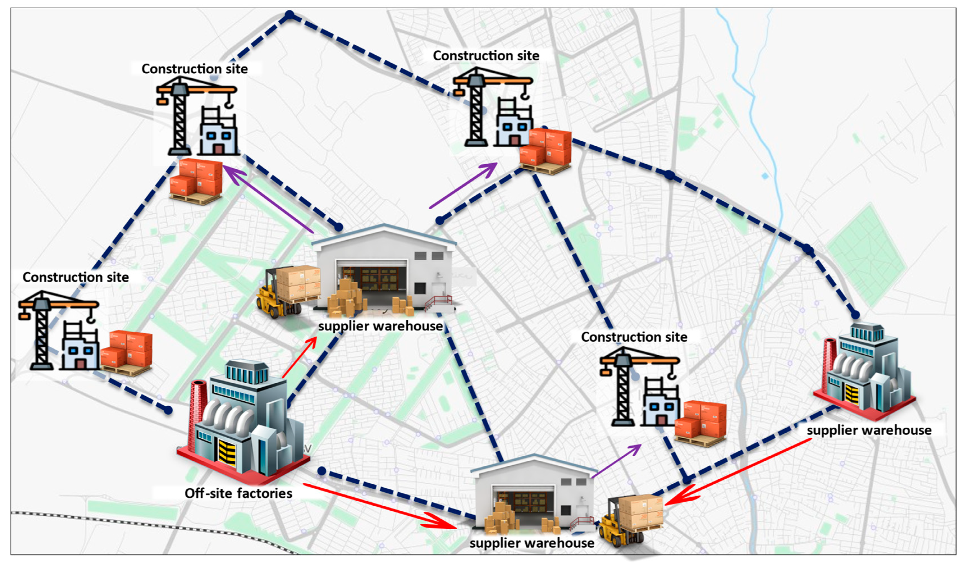
3. Problem Description

This study considers a construction project supply chain by formulating a bi-objective transportation–location–inventory–routing problem in three echelons: off-site factories, supplier warehouses, and construction sites. As the most fundamental objectives of a construction project are a limited budget and due date, our study aims to minimise the total costs of the supply chain and accelerate materials transportation. Construction phases contain components’ manufacturing and supply, stacking and logistics, and final assembly in construction locations. Therefore, the proposed supply chain includes several off-site factories that produce various types of materials and send them to open supplier warehouses and subsequently to construction sites (Figure 1). Our supply chain problem has several limitations, such as capacitated buildings and vehicles and the bounded lead times. Therefore, we determined potential capacitated supplier warehouses with specified opening costs and the optimum order amount for each component to: (i) serve the demand of their allocated construction sites and (ii) optimise the supply chain expenditures and routes for components transportation. Since unpredictable events may occur in this field, one of the elements that can be assumed as an uncertain factor in a construction project is the existence of uncertain demand, which leads to inadequate supply efficiency. To deal with the stochastic demand in customer zones, all supplier warehouses hold a specified amount of each component as safety stock to meet the construction site’s requirements with the specified service level. We also consider the stochastic capacity constraints of warehouses according to [42], with a specified value for risk level that prevents the inventory of the warehouse from exceeding a maximum value. As mentioned, another key factor in construction projects is the timeliness of the contract. To supply and access materials as quickly as possible, we need to choose routes with less time. To avoid project prolongation, we consider constraints related to average lead time at off-site factories and supplier warehouses to accelerate transferring components to construction sites considering their demand. Therefore, our proposed problem contains two-stage modelling: The first stage is called the transportation stage of TLRP, which is related to the distribution of components from off-site factories to open supplier warehouses. The second is called the routing stage that contains the distribution of components from supplier warehouses to construction sites. As we mentioned before, this study is according to an (R, s, S) inventory control policy, in which levels of inventory are checked each r period. In the condition that the inventory level is lower than s, an order is placed to reach the level of S. Therefore, the order quantity has got to consider the well-known undershoot magnitude ( U S 𝒿 𝒻 ), which is the number of items required besides s to reach S items of inventory [42].

3.1. Assumptions

Mathematical modelling techniques may successfully condense and emphasise the most relevant parts of real-world decision-making situations. However, these problems are often difficult [63]. As a result, considering all features of a real-world situation may either make a model too sophisticated to draw conclusions from or preclude an otherwise correct model from explaining empirically recognised problems. As a result, successful models depend significantly on simplifying assumptions that minimise complexity while keeping the system’s primary attributes. As a result, our mathematical modelling considers the following assumptions, resulting in a highly effective model:
  • Each supplier warehouse can store different types of components, and each type of component has a specified risk level, which is identical in all warehouses.
  • The risk level depends on the component type.
  • The amount of safety stock and reorder point depend on the component type.
  • LT depends on the origin and the destination.
  • Order quantity and LT in a supplier warehouse are estimated by weighted average.
  • Fixed ordering cost and holding cost is identical in all supplier warehouse.

3.2. Notation and Index

The sets, parameters, and variables described below are employed to formulate the problem. In addition, Appendix A provides some additional parameters for developing the model.
Sets and Parameters
𝓅 The number of off-site factories.
𝓂 The number of potential sites for supplier warehouse location.
n The number of construction sites.
𝒻 The number of components.
K = 1 , 2 , , 𝓅 Set of indexes for off-site factories.
J = 1 , 2 , , 𝓂 Set of indexes for supplier warehouses.
𝓘 = 𝓂 + 1 , 𝓂 + 2 , , 𝓂 + 𝓃 Set of indexes for construction sites.
𝓕 = 1 , 2 , , 𝒻 Set of indexes for components.
𝒶 𝓀 𝒻 Component capacity in off-site factory 𝓀 for component 𝒻.
𝒹 𝓀 𝒿 Cost of sending one truck from off-site factory 𝓀 to supplier warehouse 𝒿.
Truck capacity, off-site factory-supplier warehouse transportation stage.
𝒿 Fixed cost for opening and operating of supplier warehouse 𝒿.
𝒸 𝒾 𝒿 Cost of visiting construction site/supplier warehouse 𝒿 right after construction site/supplier warehouse 𝒾 in the route stage.
V C 𝒶 𝓅 Vehicles capacity on the route stage.
τ 𝒾 𝒿 Travelling distance from construction site/supplier warehouse 𝒾 to construction site/supplier warehouse 𝒿.
O C 𝒿 Fixed ordering cost at supplier warehouse 𝒿.
H C 𝒿 Holding cost per time unit at supplier warehouse 𝒿.
𝜇 𝒾 𝒻 Mean demand of construction site 𝒾 for component 𝒻 per day.
σ 𝒾 𝒻 Standard deviation of the demand of construction site 𝒾 for component 𝒻 per day.
I C 𝒶 𝓅 𝒿 𝒻 Capacity at supplier warehouse 𝒿 for component 𝒻.
Q C 𝒶 𝓅 𝒿 𝒻 Maximum order quantity at supplier warehouse 𝒿 for component 𝒻.
𝒿 Inventory check period at supplier warehouse 𝒿 in days.
T 𝒾 𝒿 Average lead-time at supplier warehouse 𝒿 to construction site 𝒾 in days.
T 𝓀 𝒿 Average lead-time at off-site factory 𝓀 to supplier warehouse 𝒿 in days.
1 α 𝒿 Value of service level at supplier warehouse 𝒿.
B 𝒻 Value of risk level at each supplier warehouse for component 𝒻.
T Maximum possible total traveling distance of a vehicle in the route stage.
𝓉 Transportation time unit per distance unit.
Variables
X 𝓀 𝒿 𝒻 Amount of component 𝒻 sent from off-site factory 𝓀 to supplier warehouse 𝒿.
w 𝓀 𝒿 The number of trucks sent from off-site factory 𝓀 to supplier warehouse 𝒿.
Q 𝒿 𝒻 Minimum order quantity of component f from supplier warehouse 𝒿 if D 𝒾 𝒻 0 .
Q 𝓀 𝒿 𝒻 Order quantity of component f sent from off-site factory 𝓀 to supplier warehouse 𝒿. It is greater than 0 if d 𝒿 > 0 and 0 o . w .
D 𝒿 𝒻 Total mean demand of component f at supplier warehouse 𝒿. It is greater than 0 if there exists at least one d 𝒾 𝒿 > 0 and 0 o . w .
V 𝒿 𝒻 Total variance demand of component 𝒻 at supplier warehouse 𝒿. It is greater than 0 if 𝒹 𝒿 > 0 and 0 o . w .
U 𝒾 Variable used to prevent exceeding the vehicles capacity and for sub-tour elimination. It represents the load of the vehicle after visiting construction site 𝒾.
𝒾 Variable to prevent exceeding the maximum distance constraint. It represents the distance travelled by the vehicle after visiting the construction site 𝒾.
T 𝒾 Delivery time for construction site 𝒾.
m i n Length of the shortest route.
m a x Length of the longest route.
𝓎 𝒿 { 1 0 If supplier warehouse 𝒿 is open
Otherwise
Z 𝒾 𝒿 { 1 0 If construction site 𝒾 is assigned to supplier warehouse 𝒿
Otherwise
X 0 𝒾 ( 𝒿 ) { 1 0 If construction site 𝒾 is the first construction site in any route of supplier warehouse 𝒿
Otherwise
X 𝒾 0 ( 𝒿 ) { 1 0 If construction site 𝒾 is the last construction site in any route of supplier warehouse 𝒿
Otherwise
X 𝒾 ( 𝒿 ) { 1 0 If construction site is visited just after construction site 𝒾 in any route of supplier warehouse 𝒿
Otherwise

3.3. Mathematical Formulation

For our bi-objective model, we presented the following mathematical model.
m i n 𝓯 1 = 𝓳 = 1 𝓶 ( 𝓰 𝓳 𝔂 𝓳 ) + 𝓴 K 𝓳 J 𝓭 𝓴 𝓳 𝔀 𝓴 𝓳 + 𝓳 J 𝓲 𝓘 ( C 𝓳 𝓲 X 0 𝓲 ( 𝓳 ) + C 𝓲 𝓳 X 𝓲 0 ( 𝓳 ) ) + 𝓳 J 𝓲 𝓘 l I l i C 𝓲 𝓵 X 𝓲 𝓵 ( 𝓳 ) + 𝓳 = 1 𝓶 𝓯 = 1 𝓯 ( O C 𝓳 D 𝓳 𝓯 ( Q 𝓳 𝓯 + U S 𝓳 𝓯 ) + H C 𝓳 ( Q 𝓳 𝓯 + U S 𝓳 𝓯 ) 2 ) + 𝓳 = 1 𝓶 𝓯 = 1 𝓯 ( H C 𝓳 ( D 𝓳 f R 𝓳 + Z 1 α 𝓳 R 𝓳 + W L T 𝓳 𝓯 v 𝓳 𝓯 U S 𝓳 𝓯 ) ) m i n 𝓯 2 = L m i n L m a x
Subjected to:
𝒿 J X 𝓀 𝒿 𝒻 𝒶 𝓀 𝒻 𝓀 K ,   𝒻 F (1)
𝓌 𝓀 𝒿 𝒻 F X 𝓀 𝒿 𝒻 𝓀 K ,   𝒿 J (2)
𝓀 K X 𝓀 𝒿 𝒻 𝓘 C 𝒶 𝓅 𝒿 f y 𝒿 𝒿 J ,   𝒻 F (3)
𝓀 K X 𝓀 𝒿 𝒻 = i I 𝓉 𝒾 𝒻 Z i 𝒿 𝒿 J ,   𝒻 (4)
j J Z 𝒾 𝒿 = 1 𝒾 𝓘 (5)
Z 𝒾 𝒿 = 𝓎 𝒿 𝒾 𝓘 ,   𝒿 J (6)
i I 𝓍 0 𝒾 ( 𝒿 ) = i I 𝓍 𝒾 0 ( 𝒿 ) 𝒿 J (7)
i I { 0 } l i x 𝒾 ( 𝒿 ) = Z 𝒿 𝓘 ,   𝒿 J (8)
l I { 0 } l i x 𝒾 ( 𝒿 ) = Z 𝒾 𝒿 𝒾 𝓘 ,   𝒿 J (9)
u 𝒾 u 1 + V C 𝒶 𝓅 j J x i l ( j ) V C 𝒶 𝓅 f F 𝜇 𝒾 𝒻 𝒾 , 𝓘 , i l (10)
f F μ 𝓲 𝓯 𝓾 𝓲 V C 𝒶 𝓅
𝒾 𝓘 (11)
e 𝒾 e + ( T + τ 𝒾 ) 𝒿 J x 𝒾 ( 𝒿 ) + ( T τ 𝒾 ) 𝒿 J X 𝒿 ( 𝒿 ) T 𝒾 , 𝓘 , 𝒾 (12)
𝒿 J τ 𝒿 𝒾 x 0 𝒾 ( 𝒿 ) e 𝒾 T + 𝒿 J ( τ 𝒿 𝒾 T ) x 0 𝒾 ( 𝒿 ) 𝒾 𝓘 (13)
e 𝒾 T 𝒿 J τ 𝒾 𝒿 x 𝒾 0 ( 𝒿 ) 𝒾 𝓘 (14)
L m a x e 𝓲 + 𝓳 J τ 𝓲 𝓳 x 𝓲 0 ( 𝓳 )
𝒾 𝓘 (15)
m i n e 𝒾 + 𝒿 J ( τ 𝒾 𝒿 T ) 𝓍 𝒾 0 ( 𝒿 ) + T 𝒾 𝓘 (16)
Q 𝒿 𝒻 + D 𝒿 𝒻 𝒿 + ( Z 1 α 𝒿 + 𝒿 + W T 𝒿 𝒻 + Z 1 𝒻 W T 𝒿 𝒻 ) V 𝒿 𝒻 𝓘 C 𝒶 p 𝒿 𝒻 y 𝒿 𝒿 J ,   𝒻 (17)
W T 𝒿 𝒻 = 𝓀 K T 𝓀 𝒿 X 𝓀 𝒿 𝒻 𝓀 K X 𝓀 𝒿 𝒻 𝒿 J ,   𝒻 (18)
D 𝒿 𝒻 = i = 1 𝓃 𝓉 𝒾 𝒻 Z i 𝒿 𝒿 J ,   𝒻 (19)
V 𝒿 𝒻 = i = 1 𝓃 σ 𝒾 𝒻 2 Z 𝒾 𝒿 𝒿 J ,   𝒻 (20)
𝓉 e 𝒾 T 𝒾 𝒿 Z 𝒾 𝒿 + ( 1 Z 𝒾 𝒿 ) 𝒾 𝓘 ,   𝒿 J (21)
𝒾 𝒻 μ 𝒾 𝒻 T 𝒾 𝒾 𝒻 μ 𝒾 𝒻 𝒹 𝓉 (22)
T 𝒾 𝒿 T 𝒾 𝒿 Z 𝒾 𝒿 𝒾 𝓘 (23)
𝓀 Q 𝓀 𝒿 𝒻 = Q 𝒿 𝒻 + U S 𝒿 𝒻 𝒿 J , 𝒻 (24)
Q 𝓀 𝒿 𝒻 𝒿 = X 𝓀 𝒿 𝒻 𝓀 K , 𝒿 J , 𝒻 (25)
U S 𝒿 𝒻 = { V 𝒿 𝒻 2 D 𝒿 𝒻 + j 2 D 𝒿 𝒻 ,   D 𝒿 𝒻 0 0       , o . w 𝒿 J ,   𝒻 (26)
u 𝒾 0 ; e 𝒾 0 𝒾 𝓘 (27)
𝓎 𝒿 { 0 , 1 } 𝒿 J
Z 𝒾 𝒿 { 0 , 1 } ; x 0 𝒾 ( 𝒿 ) { 0 , 1 } ; x 𝒾 0 ( 𝒿 ) x 0 𝒾 ( 𝒿 ) 𝒾 𝓘 ,   𝒿 J
X 𝓀 𝒿 𝒻 0 ; 𝓌 𝓀 𝒿 Z + 𝓀 K ,   𝒿 J
x 𝒾 ( 𝒿 ) { 0 , 1 } 𝒾 , 𝓘 , 𝒾 ,   𝒿 J
m a x 0 ; m i n 0
The first objective function minimises the transportation, installation, ordering, and holding costs and the second one represents a well-balanced set of routes. Constraint (1) ensures not exceeding the off-site factories’ capacity. Constraint (2) links the number of components sent from each off-site factory to each supplier warehouse with the capacity of the trucks. Constraint (3) prevents exceeding each supplier warehouse capacity. Constraint (4) guarantees that the amount of each component sent to each supplier warehouse must exactly be the same as the sum of the mean demands of all construction sites assigned to each supplier warehouse for each component. Constraint (5) ensures that each construction site is assigned to a single supplier warehouse. Constraint (6) certifies that the construction sites are only assigned to the created warehouse. Constraint (7) imposes that the number of vehicles leaving a supplier warehouse must equal the number of vehicles returning to that supplier warehouse. Constraints (8) and (9), first, compel that each construction site must be visited only after one supplier warehouse or after another construction site. Second, these constraints enable the routing infrastructure only between construction sites allocated to the identical supplier warehouse. Intending to avoid exceeding vehicle capacities, as well as the sub-tours existence, constraints (10) and (11) are considered. These constraints originate from the travelling salesman problem to eliminate classical sub-tour obstacles [64]. We develop the formation of open paths with the capacity limitation related to assigned construction sites, in which the sum of demands should be lower than V C 𝒶 𝓅 . Taking the second objective function into account, constraints (12), (13), and (14) guarantee the variable e 𝒾 to obtain the optimum value of the distance travelled by the vehicle after visiting construction site 𝒾. In constraint (12), variable e indicates the length of the route until construction site 𝓵. Then, variable e 𝒾 is compelled to take the value of τ 𝒾 𝒿 when construction site 𝒾 is the first in a route of supplier warehouse 𝒿 (constraint (13)), while constraint (14) actives the exceeding prevention of the maximum length limit 𝓉 . Constraint (15) is required to calculate the longest route in the routing phase. When construction site 𝒾 is the last in a route of supplier warehouse 𝒿 , variable x 𝒾 0 ( 𝒿 ) takes the value of 1. For other construction sites on the same route, the values of e 𝒾 + 𝒿 J τ 𝒾 𝒿 x 𝒾 0 ( 𝒿 ) will always be lower than the one for the last construction site. Therefore, the greater the value of e 𝒾 + τ 𝒾 𝒿 , the longer route will be created. Constraint (16) determines the routing stage to obtain the shortest route. If construction site 𝒾 is not the last in a route, the variables x 𝒾 0 ( 𝒿 ) are always zero; therefore, the expression e 𝒾 + T is greater than the duration of any route. If construction site 𝒾 is the last in a route of supplier warehouse 𝒿 , then x 𝒾 0 ( 𝒿 ) = 1 , having as a result m i n e 𝒾 + τ 𝒾 𝒿 . Note that the objective that minimises 𝒻 2 = m a x m i n forces m a x to obtain the lowest possible value (duration of the longest route), and L m i n takes the greatest possible value (duration of the shortest route) [51]. Constraint (17) ensures that the supplier warehouse’s capacity does not exceed the upper line. Constraint (18) represents the average weighted delivery time. Constraints (19) and (20) show the variance and mean demand for component 𝒻 in supplier warehouse 𝒿 . Constraint (22) ensures that W T 𝒿 𝒻 for each construction site 𝒾 does not exceed the appropriate level and makes construction sites with more demands have less T 𝒾 𝒿 . Constraint (23) is related to the delivery time for each construction site 𝒾 . Constraints (24) and (25) balance the amount of input and output components for each supplier warehouse and off-site factory. Constraint (26) represents the amount of decrease in inventory level s at the ordering time. Constraint (27) defines the type of variables that are used.

4. Solution Method

The proposed model includes two objective functions to be minimised. We can apply the exact, heuristic, or meta-heuristic approaches to solve the mathematical models. Regarding the NP-hard nature of the problems, the solutions of large instances might be inappropriate, especially related to the considerable solving time. Therefore, heuristic or meta-heuristic approaches are recommended to be utilised to achieve near-optimal answers in a reasonable time. Many real-world optimisation problems are difficult, notably in the construction sector [4]. Meta-heuristic algorithms may be utilised to solve these difficult problems [65,66]. There are several advantages of employing meta-heuristic algorithms [67,68]. They can be applied to any problem that can be expressed as a function optimisation problem [69], are typically easier to understand and implement [70], can solve larger problems faster [71], are simple to design and implement [72], are very flexible [73,74], and can be combined with other techniques [75]. Accordingly, we solve the bi-objective model in two sizes in order to evaluate the applicability of the proposed problem. The exact method solves the small size instance using Generalised Algebraic Modelling System (GAMS) software’s BARON and provides optimal solutions. Moreover, a Grasshopper Optimisation Algorithm (GOA) is applied to solve large sample problems.

4.1. Multi-Objective Approach

In order to obtain the optimum solution of our bi-objective mathematical model, we apply the L P - metric method for small and large problems, respectively, which gathers two conflicting objectives and normalises them into one function [76]. The approach in the L P - metric method defines the summation of the weights ( 𝓈 i   ) , which are multiplied by every normalised objective function ( Z i n o r m ) . In this study, given both objective functions are to be minimised, we have:
Min   Z t o t a l = 𝓈 1   Z 1 n o r m + ( 1 𝓈 1   ) Z 2 n o r m
Owing to minimising both objective functions, the normalised values of Z i are obtained from the equation below:
Z i n o r m = Z i Z i m i n Z i m a x Z i m i n
Due to the importance of each objective function and the decision maker’s preference, the weights will be determined. To attain Pareto optimal solutions, a dispersed weighted vector was produced [77].

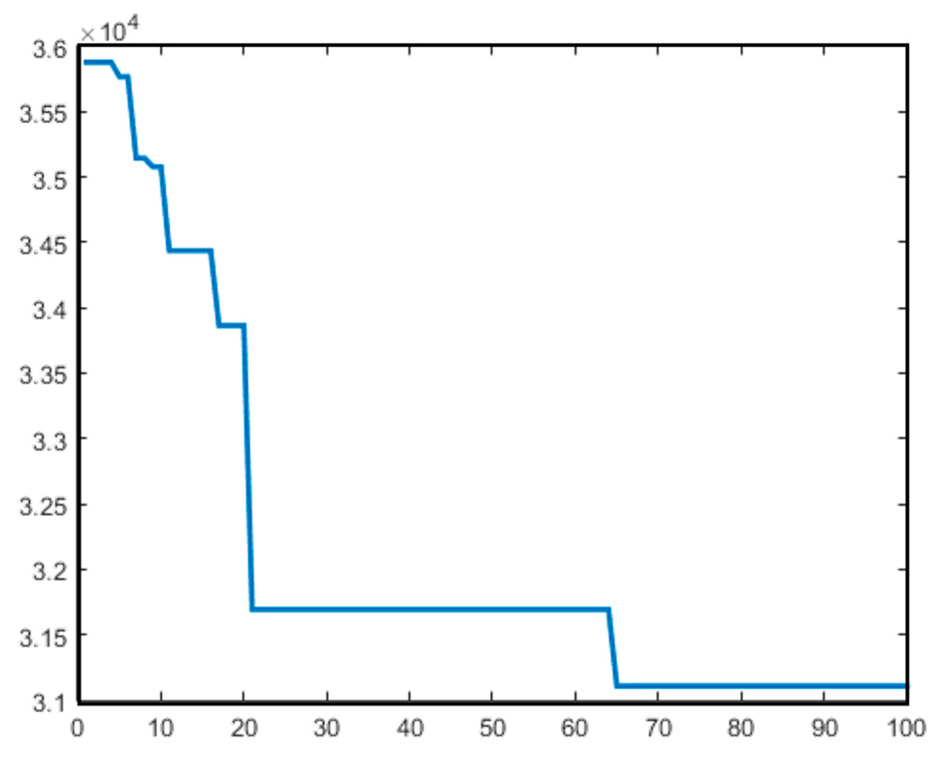
4.2. Grasshopper Optimisation Algorithm (GOA)

The GOA algorithm is proposed by Saremi et al. [78], which is a meta-heuristic optimisation method inspired by grasshoppers’ group behaviour. This method imitates and simulates the behaviour of grasshoppers in nature and their group movement towards food sources [79]. The capability of GOA in tackling complex problems has been proven by numerous studies [80,81,82].
Three factors affect the grasshopper movement, including social interaction ( S o i ), the wind advection ( A d i ), and the gravity force ( G f i ). The representation position for the i-th grasshopper ( X i ) is defined by the following equation:
X i = S o i + G f i + A d i
where S o i is defined as:
S o i = j = 1 , j i H S ( | X j X i | ) X j X i d i j
In the above equation, S is a function that is defined as follows ( k and u are constant parameters):
S ( t ) = k × e t u e t
In addition, d i j = | X j X i | and H   are the quantity of grasshoppers in the swarm. In addition, in Equation (30) G f i = g r × e ^ g r , where g r is a constant parameter and e ^ g r is a unity vector. Furthermore, A d i = h × e ^ w d where h is a constant parameter and e ^ w d is a unity vector. According to Saremi, Mirjalili, and Lewis [78], Equation (30) can be modified to reflect the actual conditions of the grasshoppers’ movement, and it is represented as follows:
X i k = K ( j = 1 , j i H K u b k l b k 2 S ( | x j k x i k | ) x j x i d i j ) + T k
where u b k   and   l b k denote the upper bound and lower bound, respectively. T k   is defined as the value of the k -th dimension in the target, while K is defined as:
K = K m a x i × K m a x K m i n I m
In general, the GOA steps are as Algorithm 1.
Algorithm 1 Grasshopper Optimisation Algorithm
1: Input: The position of grasshoppers X i (i = 1, 2…, H), the boundaries, I m , K m a x , K m i n
2: Output: the best solution (A)
3: While i I m   d o
4: Update the value of K by using the Equation (34).
   5: For each position do
         6: Normalised the distance between grasshoppers.
         7: Update the current position of the individual by the Equation (33).
         8: The current search agent will be brought back if it is outside the boundaries.
         9: If a better solution becomes available, A is updated.
   10: Endfor
   11: i = i + 1
12: Endwhile
13: Return A
As our model is an NP-hard problem, we use a meta-heuristic algorithm to solve the large size problem. The GOA is submitted as one of the optimisers. Hence the optimal results of the small instance were almost similar to solutions provided by the GOA algorithm, which means the GOA algorithm would be appropriate for large size instances.

5. Numerical Results

The model is validated by some test problems to verify the effectiveness of the proposed supply chain model. Therefore, small and large-size instances are provided to be solved. As the number of facilities increases, it takes longer to solve the problem. In addition, solving NP-hard problems with exact algorithms are difficult and time-consuming. Therefore, applying the GOA algorithm for this problem is an appropriate solution. The information about small and large-size instances is as follows:

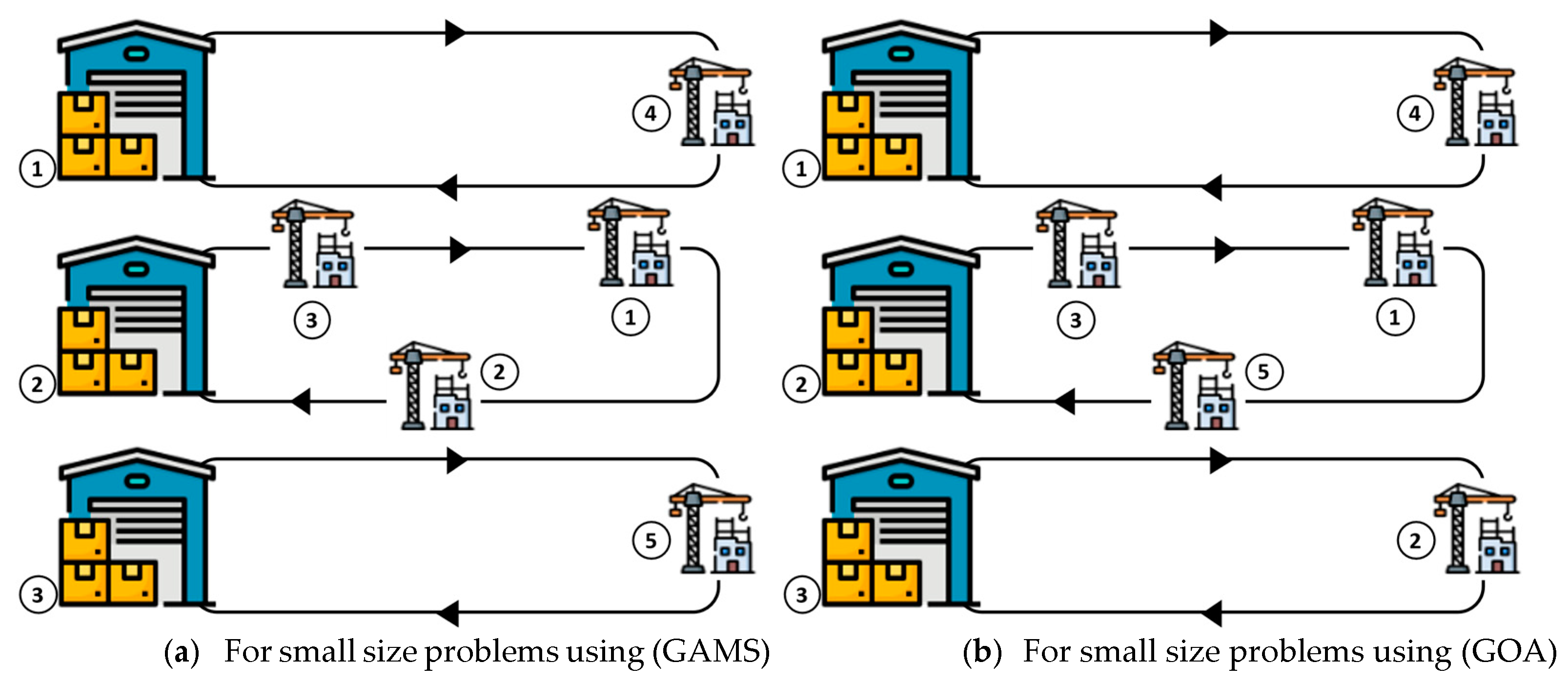
5.1. Small-Size Sample Problem

Five construction sites are considered for the small-size problem, and their demand for two components are supplied by three supplier warehouses that buy components from two off-site factories. Table 1 illustrates the input data used for parameters, and Table 2 shows the optimal results obtained by GAMS and GOA. We run the GOA five times, and the results demonstrate that the amounts of variables that GAMS obtain are virtually similar to the GOA results. Therefore, the presented GOA algorithm is efficient and can be applied to large-size problems.
Figure 2 shows the allocation of construction sites to each supplier warehouse and depicts the routes between the supplier warehouses and construction sites for sample small-size problems obtained by GAMS and GOA.
In a multi-objective approach, we solve the problem by dispersing weighted vectors. Pareto optimal solutions are calculated by assigning different weights. Pareto solutions indicate that there is a set of solutions that have no preference for each other, so we do not have a unique optimal solution. We prepare a set of solutions based on the decision maker’s preferences and real-world conditions in these problems. Table 3 disperses the weighted vectors presented. The first row of Table 3 depicts the weights assigned to the first objective function and the second row implies the weights assigned to the second objective function. The problem is solved for each value, and the results are available in Table 4.

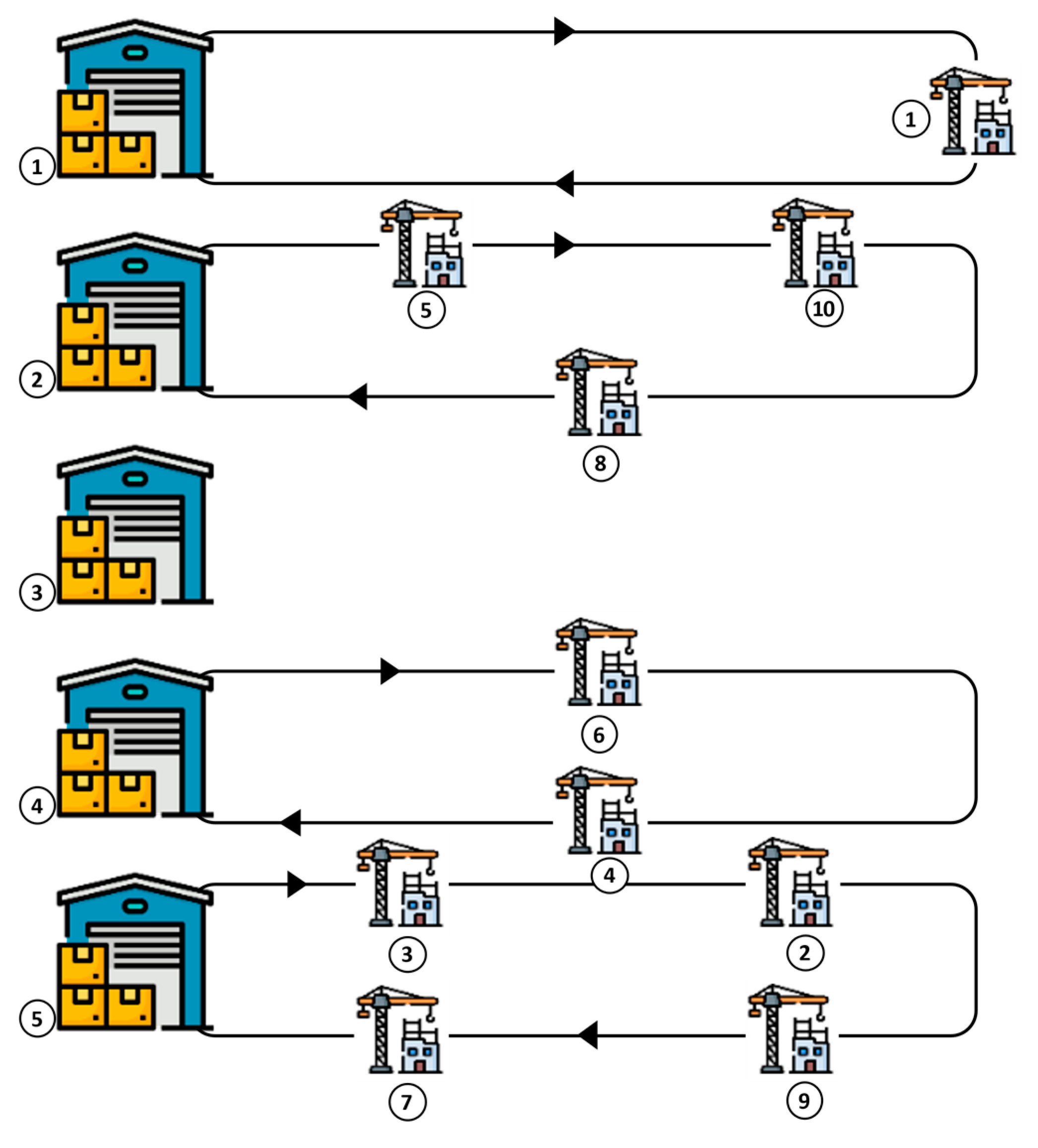
5.2. Large-Size Sample Problem

To define the problem at a large size, ten construction sites are considered, and their demands for four components are supplied by five supplier warehouses, which buy components from four off-site factories. GOA is applied to the data, and results are reported in Table 5, Table 6, Table 7 and Table 8.
Figure 3 shows the convergence of the GOA algorithm with the optimal solutions, and Figure 4 shows the allocation of construction sites to each supplier warehouse and depicts the routes between supplier warehouses and the construction sites for large-size sample problems. As we see, supplier warehouse three did not open, and construction sites were assigned to the rest of the supplier warehouses.

6. Sensitivity Analysis

Sensitivity analysis for some parameters is important because it can provide a profitable insight. The solution data shows that total costs increase by increasing the review period (Figure 5). Actually, in order to prevent inventory shortages when the review period increases, more safety stock should be maintained; therefore, holding costs will increase. Furthermore, by increasing the review period, the order quantity needs to be increased to meet the demands in a longer period. As a result, the amount of inventory in warehouses increases, and given the fact that each warehouse has a maximum capacity limit, more warehouses have to be created. Therefore, by increasing the review period, inventory costs will increase, excessive warehouses will be created, and finally, the total costs will increase.
As the review periods increase, the time interval between two consecutive inventory checks increases. Sequentially, the time interval between two consecutive orders will increase. Therefore, it is required to maintain more safe stock in order to meet the construction sites’ demand over a longer period. As we see in Figure 6, the solution data shows that by increasing the review period, the amount of safety stock will increase in order to meet demand.
Similar to the above analysis, by increasing the review period, order quantity will increase as much as the capacity of each supplier warehouse allows and if it exceeds the capacity of each supplier warehouse, then the new supplier warehouse will be opened. Therefore, the order quantity will decrease because more supplier warehouses supply consumers’ demand. Again, by increasing the review period, the order quantity increases as much as the capacity of existing supplier warehouses allows and again, when the amount of inventory reaches the capacity of existing supplier warehouses, a new supplier warehouse will be opened, and the order quantity in supplier warehouses will be reduced because there are more supplier warehouses. This trend is shown in Figure 7.
If the supplier warehouses have more capacity, the constraint that is related to supplier warehouse capacity becomes more relaxed. Therefore, the feasible region becomes greater, and the possibility of finding the optimal solutions increases. Therefore, the objective function can be improved. In practice, when supplier warehouse capacity increases, the number of supplier warehouses that need to be opened will be reduced. Therefore, the high cost of establishing supplier warehouses will decrease. Furthermore, construction sites will be assigned to fewer supplier warehouses when the number of opened supplier warehouses decreases, which reduces routing costs. For example, when two construction sites are assigned to one supplier warehouse, the vehicle can meet them in one trip, without returning to the supplier warehouse, while if two construction sites are assigned to two different supplier warehouses, it needs two vehicles to move from each supplier warehouse in order to supply construction sites’ demand. Therefore, by increasing each supplier warehouse’s capacity, the value of the objective function will decrease nonlinearly, but the number of supplier warehouses cannot be less than a specific amount because, for supplying construction sites, a minimum number of supplier warehouses need to be open and each supplier warehouse has its specific routes in order to supply construction sites’ demand. Therefore, more reduction in the number of supplier warehouses is not possible by further increasing the supplier warehouse’s capacity. As we see in Figure 8, improving the amount of objective function continues up to a specific amount.
As is expected, the possibility of assurance from inventory level increases as the amount of service level rises. Therefore, the amount of safety stock must be increased in order to reduce the inventory shortage. Therefore, by increasing the amount of safety stock, maintenance costs will grow up. Additionally, the number of supplier warehouses may increase due to the limited supplier warehouse’s capacity. This will add fixed costs of establishing more supplier warehouses, and consequently, routing costs will increase. As we see in Figure 9, the solution data illustrates that total costs will rise by enhancing the service level. As we see in Figure 10, the higher the service level, the greater the safety stock will be. In other words, by enhancing the service level, the company’s commitment to meet demand increases, so the amount of safety stock must be increased to supply demands to the greatest extent. When the weighted average lead time increases, it means that receiving components from the off-site factories to supplier warehouses will take longer. This will bring about the increment in delivery times for construction sites, which are shown in Figure 11.

7. Discussion and Managerial Insights

In this section, the behaviour of the model in regards to parameter changing is analysed to obtain a considerable managerial insight. Although Martínez-Salazar, Molina, Ángel-Bello, Gómez and Caballero [51], and Ghomi and Asgarian [61] mentioned some analyses, the gaps of the (R, s, S) inventory control system by consideration of supplier warehouses’ service level and construction sites’ lead-times are fulfilled in this study. Because article [58] considered the certain demand of each construction site, safety stock is not accurate in the model. Therefore, the results of sensitivity analysis are confined to the impacts of lost sales and holding costs on total costs. In addition to considering uncertainty like many papers, e.g., [83,84,85], demand is uncertain in this study, (R, s, S) inventory replenishment is considered.
Due to the acquired results, one of the key factors in inventory management is the review period. According to Figure 6, Figure 7 and Figure 8, the longer the review period assumed, the more order quantity and more safety stock to tackle uncertain demand required. Subsequently, the holding costs and the establishment outlays of more supplier warehouses are derived, which cause higher total costs. Therefore, it is better for managers to consider a short review period. On the other hand, as the review period becomes shorter, there is a shift to inventory policies with a continuous review that increases review costs. Therefore, management should consider an optimal value for the review period that balances inventory costs and the inventory review.
On the other side, considering the capacitated structures and vehicles, as well as specific service levels of supplier warehouses, is a real-world condition in which managers should handle their decisions, and in this study, it has been addressed, unlike article [58]. According to Figure 9, it is clear that increasing the capacity of distribution centres does not always improve the objective function. Due to the volume of demand that construction sites have and each distribution centre’s logistics, a minimum capacity of distribution centres is required. Therefore, the capacity limit at which each distribution centre can reduce the objective function will be very important for management to avoid additional costs. In other words, the higher the capacity of supplier warehouses is, the less number of distribution centres, and consequently, the fewer establishment costs in addition to routing outlays will be. However, to satisfy the proper routing problem by determining several road networks, the number of supplier warehouses cannot be less than a specific quantity. Furthermore, the limitation of each construction site due to its lead-time makes the managers open the optimum number of supplier warehouses to reduce the total costs and gain the most construction sites’ satisfaction simultaneously. Moreover, other economic and managerial implications can be presented as:
Managers must shorten the review period in order to reduce inventory costs. Managers can also reduce warehouse inventory stock by shortening the review period. Furthermore, by increasing the amount of safety stock inventory, managers can reduce the number of inventory inspections and, as a result, inspection costs. Furthermore, increasing the order quantity reduces inventory inspection costs while increasing inventory maintenance costs. The model developed in this study can assist managers in determining the optimal amount of order quantity and the interval between inventory inspections. Furthermore, as shown in Figure 6, if managers are unable to extend the review period, the total cost will rise. As a result, according to Figure 9, they must increase warehouse capacity in order to reduce costs. Furthermore, as shown in Figure 10 and Figure 11, if managers had increased the service level, they would have invested more in increasing the inventory level. To compensate, they can increase the capacity of warehouses, lowering total costs.

8. Conclusions and Future Directions

More companies are adopting off-site construction because of the advantages of preparing construction components in a controlled manufacturing environment. However, component supply chain issues, on the other hand, remain unresolved. Because of this, an off-site construction supply chain management model with stochastic constraints is proposed using a three-echelon supply chain management model. In this paper, multiple off-site factories produce various components and ship them to supplier warehouses in order to meet the needs of construction sites. In the proposed model, the first objective represents the costs, and the second represents the balance of drivers’ workloads. We develop an MINLP model based on a periodic inventory review policy (R, s, S), in which multi-suppliers send different components to supplier warehouses to satisfy the demands. The model was an NP-hard one; therefore, the GOA algorithm was applied to solve the large-size problem. We solved a sample small-size problem by both GAMS and GOA. The results were almost similar, suggesting that the proposed GOA algorithm is appropriate for solving large-size problems.
In this paper, we simultaneously consider different dimensions of an off-site construction project in the real world, such as multiple suppliers, multiple components, routing problems, ordering systems in the warehouses, which have not been considered in previous work. The results illustrate that with the prolongation of the review period, the safety stock in each supplier warehouse increases to the maximum capacity of each supplier warehouse, and subsequently, order quantity will increase, which raises the total costs. Moreover, the solution data demonstrates that by enhancing the service level, more safety stock is needed, and subsequently, the total costs will increase.

Author Contributions

Conceptualisation S.A.-S.S., H.M., A.A. and F.J.; data curation S.A.-S.S., H.M., A.A. and S.J.; formal analysis S.A.-S.S. and H.M.; funding acquisition F.J. and M.Y.; investigation S.A.-S.S., H.M., A.A. and S.J.; methodology S.A.-S.S., H.M. and S.J.; project administration A.A., F.J. and S.J.; resources S.A.-S.S., H.M. and S.J.; software S.A.-S.S. and H.M.; supervision A.A., F.J. and M.Y.; validation S.A.-S.S., H.M. and A.A.; visualisation S.A.-S.S., H.M., S.J. and M.Y.; writing—original draft S.A.-S.S., H.M. and S.J.; writing—review and editing A.A., F.J. and M.Y. All authors have read and agreed to the published version of the manuscript.

Funding

This research received no external funding.

Institutional Review Board Statement

Not applicable.

Informed Consent Statement

Not applicable.

Data Availability Statement

The data used in the study is available with the authors and can be shared upon reasonable requests.

Conflicts of Interest

The authors declare no conflict of interest.

Appendix A

We define U S 𝒿 𝒻 as follows [42]:
U S 𝒿 𝒻 = V 𝒿 𝒻 2 D 𝒿 𝒻 + 𝒿 D 𝒿 𝒻 2
Therefore, when an order arrives at supplier warehouse 𝒿 , the inventory level becomes s 𝒻 U S 𝒻   and the order quantity would be S 𝒻 𝓈 𝒻 + U S 𝒻 .
Demand during LT for component 𝒻 at supplier warehouse 𝒿 is:
𝒾 S D 𝒾 𝒻 ( W T 𝒿 𝒻 ) = S D 𝒿 𝒻 ( T )
We let T = W T 𝒿 𝒻 , the maximum inventory level of component 𝒻 at ordering time is calculated as follows:
𝓈 𝒻 U S 𝒻 + S 𝒻 𝓈 𝒻 U S 𝒻 S D 𝒻 ( T ) = S 𝒻 S D 𝒻 ( T )
Therefore, for each supplier warehouse, we have:
S 𝒿 𝒻 S D 𝒿 𝒻 ( T ) = I 𝓂 𝒶 𝓍 𝒿 𝒻
In order to satisfy the capacity constraint for each supplier warehouse, we have:
P ( 𝓘 𝓂 𝒶 𝓍 𝒿 𝒻 𝓘 𝒸 𝒶 𝓅 𝒿 𝒻 ) 𝛽 𝒻
Substituting Equation (A1) into Equation (A2) results in Equation (A3), as follows:
P ( S 𝒿 𝒻 S D 𝒿 𝒻 ( T ) ) I C 𝒶 𝓅 𝒿 𝒻 ) 𝛽 𝒻
Similar to [86], after some algebra we have:
S 𝒿 𝒻 𝓘 𝒸 𝒶 𝓅 𝒿 𝒻 + ( D 𝒿 𝒻 W T 𝒿 𝒻 ) Z 1 𝛽 𝒻 W T 𝒿 𝒻 V 𝒿 𝒻
and similar to [42], we have:
S 𝒿 𝒻 = Q 𝒿 𝒻 + 𝓈 𝒿 𝒻
Because s 𝒿 𝒻 is the reorder point for product f in supplier warehouses 𝒿 , the demand must be satisfied during W L T 𝒾 𝒻 + R 𝒾 . Therefore, by considering the service level for supplier warehouse 𝒿 we have:
P ( S D 𝒾 𝒻 ( W T 𝒿 𝒻 + 𝒿 ) 𝓈 𝒿 𝒻 ) = 1 𝛼 𝒿
After some algebra, the reorder point is computed as follows:
𝓈 𝒿 𝒻 = D 𝒿 𝒻 ( W T 𝒿 𝒻 + 𝒿 ) + Z 1 𝛼 𝒾 ( W T 𝒿 𝒻 + 𝒿 ) V 𝒿 𝒻
In respect to Equations (4), (5) and (7), the capacity constraint for component 𝒻 in supplier warehouses 𝒿 is calculated as follows:
Q 𝒿 𝒻 + D 𝒿 𝒻 ( 𝒿 ) + ( Z 1 𝛼 𝒿 ( W T 𝒿 𝒻 + 𝒿 ) + Z 1 𝛽 𝒻 W T 𝒿 𝒻 ) V 𝒿 𝒻 𝓘 𝒸 𝒶 𝓅 𝒿 𝒻
Safety stock is equal to average inventory just before an order arrives, so we have:
S S 𝒿 𝒻 = E ( 𝓘 𝒿 𝒻 ) = E ( s 𝒿 𝒻 U S 𝒿 𝒻 S D ( W T 𝒿 𝒻 ) ) = 𝓈 𝒿 𝒻 U S 𝒿 𝒻 D 𝒿 𝒻 W T 𝒿 𝒻
Finally, by replacing Equation (A7) in Equation (A9) we have:
S S 𝒿 𝒻 = D 𝒿 𝒻 𝒿 + Z 1 𝛼 i ( W T 𝒿 𝒻 + 𝒿 ) V 𝒿 𝒻 U S 𝒿 𝒻

References

  1. Kabirifar, K.; Mojtahedi, M.; Wang, C.; Tam, V.W.Y. Construction and demolition waste management contributing factors coupled with reduce, reuse, and recycle strategies for effective waste management: A review. J. Clean. Prod. 2020, 263, 121265. [Google Scholar] [CrossRef]
  2. Shahmansouri, A.A.; Yazdani, M.; Hosseini, M.; Akbarzadeh Bengar, H.; Farrokh Ghatte, H. The prediction analysis of compressive strength and electrical resistivity of environmentally friendly concrete incorporating natural zeolite using artificial neural network. Constr. Build. Mater. 2022, 317, 125876. [Google Scholar] [CrossRef]
  3. Ghafourian, K.; Kabirifar, K.; Mahdiyar, A.; Yazdani, M.; Ismail, S.; Tam, V.W.Y. A synthesis of express analytic hierarchy process (EAHP) and partial least squares-structural equations modeling (PLS-SEM) for sustainable construction and demolition waste management assessment: The case of Malaysia. Recycling 2021, 6, 73. [Google Scholar] [CrossRef]
  4. Yazdani, M.; Kabirifar, K.; Frimpong, B.E.; Shariati, M.; Mirmozaffari, M.; Boskabadi, A. Improving construction and demolition waste collection service in an urban area using a simheuristic approach: A case study in Sydney, Australia. J. Clean. Prod. 2021, 280, 124138. [Google Scholar] [CrossRef]
  5. Kabirifar, K.; Mojtahedi, M.; Wang, C.C. A systematic review of construction and demolition waste management in Australia: Current practices and challenges. Recycling 2021, 6, 34. [Google Scholar] [CrossRef]
  6. Mirmozaffari, M.; Yazdani, M.; Boskabadi, A.; Dolatsara, H.A.; Kabirifar, K.; Golilarz, N.A. A novel machine learning approach combined with optimization models for eco-efficiency evaluation. Appl. Sci. 2020, 10, 5210. [Google Scholar] [CrossRef]
  7. Shahmansouri, A.A.; Akbarzadeh Bengar, H.; AzariJafari, H. Life cycle assessment of eco-friendly concrete mixtures incorporating natural zeolite in sulfate-aggressive environment. Constr. Build. Mater. 2021, 268, 121136. [Google Scholar] [CrossRef]
  8. Shahmansouri, A.A.; Yazdani, M.; Ghanbari, S.; Akbarzadeh Bengar, H.; Jafari, A.; Farrokh Ghatte, H. Artificial neural network model to predict the compressive strength of eco-friendly geopolymer concrete incorporating silica fume and natural zeolite. J. Clean. Prod. 2021, 279, 123697. [Google Scholar] [CrossRef]
  9. Wei, W.; Mojtahedi, M.; Yazdani, M.; Kabirifar, K. The Alignment of Australia’s National Construction Code and the Sendai Framework for Disaster Risk Reduction in Achieving Resilient Buildings and Communities. Buildings 2021, 11, 429. [Google Scholar] [CrossRef]
  10. Shahmansouri, A.A.; Akbarzadeh Bengar, H.; Ghanbari, S. Compressive strength prediction of eco-efficient GGBS-based geopolymer concrete using GEP method. J. Build. Eng. 2020, 31, 101326. [Google Scholar] [CrossRef]
  11. Yazdani, M.; Kabirifar, K.; Fathollahi-Fard, A.M.; Mojtahedi, M. Production scheduling of off-site prefabricated construction components considering sequence dependent due dates. Environ. Sci. Pollut. Res. 2021, 1–17. [Google Scholar] [CrossRef] [PubMed]
  12. Hussein, M.; Zayed, T. Critical factors for successful implementation of just-in-time concept in modular integrated construction: A systematic review and meta-analysis. J. Clean. Prod. 2021, 284, 124716. [Google Scholar] [CrossRef] [PubMed]
  13. Tsz Wai, C.; Wai Yi, P.; Ibrahim Olanrewaju, O.; Abdelmageed, S.; Hussein, M.; Tariq, S.; Zayed, T. A critical analysis of benefits and challenges of implementing modular integrated construction. Int. J. Constr. Manag. 2021, 1–24. [Google Scholar] [CrossRef]
  14. Shahpari, M.; Saradj, F.M.; Pishvaee, M.S.; Piri, S. Assessing the productivity of prefabricated and in-situ construction systems using hybrid multi-criteria decision making method. J. Build. Eng. 2020, 27, 100979. [Google Scholar] [CrossRef]
  15. Tam, V.W.Y.; Fung, I.W.H.; Sing, M.C.P.; Ogunlana, S.O. Best practice of prefabrication implementation in the Hong Kong public and private sectors. J. Clean. Prod. 2015, 109, 216–231. [Google Scholar] [CrossRef]
  16. Monahan, J.; Powell, J.C. An embodied carbon and energy analysis of modern methods of construction in housing: A case study using a lifecycle assessment framework. Energy Build. 2011, 43, 179–188. [Google Scholar] [CrossRef]
  17. Hussein, M.; Eltoukhy, A.E.E.; Darko, A.; Eltawil, A. Simulation-Optimization for the Planning of Off-Site Construction Projects: A Comparative Study of Recent Swarm Intelligence Metaheuristics. Sustainability 2021, 13, 13551. [Google Scholar] [CrossRef]
  18. Hussein, M.; Eltoukhy, A.E.E.; Karam, A.; Shaban, I.A.; Zayed, T. Modelling in off-site construction supply chain management: A review and future directions for sustainable modular integrated construction. J. Clean. Prod. 2021, 310, 127503. [Google Scholar] [CrossRef]
  19. Hsu, P.-Y.; Angeloudis, P.; Aurisicchio, M. Optimal logistics planning for modular construction using two-stage stochastic programming. Autom. Constr. 2018, 94, 47–61. [Google Scholar] [CrossRef]
  20. Li, J.-Q.; Han, Y.-Q.; Duan, P.-Y.; Han, Y.-Y.; Niu, B.; Li, C.-D.; Zheng, Z.-X.; Liu, Y.-P. Meta-heuristic algorithm for solving vehicle routing problems with time windows and synchronized visit constraints in prefabricated systems. J. Clean. Prod. 2020, 250, 119464. [Google Scholar] [CrossRef]
  21. Jeong, J.; Hong, T.; Ji, C.; Kim, J.; Lee, M.; Jeong, K.; Lee, S. An integrated evaluation of productivity, cost and CO2 emission between prefabricated and conventional columns. J. Clean. Prod. 2017, 142, 2393–2406. [Google Scholar] [CrossRef]
  22. Zhai, Y.; Zhong, R.Y.; Li, Z.; Huang, G. Production lead-time hedging and coordination in prefabricated construction supply chain management. Int. J. Prod. Res. 2017, 55, 3984–4002. [Google Scholar] [CrossRef]
  23. Zhai, Y.; Zhong, R.Y.; Huang, G.Q. Buffer space hedging and coordination in prefabricated construction supply chain management. Int. J. Prod. Econ. 2018, 200, 192–206. [Google Scholar] [CrossRef]
  24. Kong, L.; Li, H.; Luo, H.; Ding, L.; Zhang, X. Sustainable performance of just-in-time (JIT) management in time-dependent batch delivery scheduling of precast construction. J. Clean. Prod. 2018, 193, 684–701. [Google Scholar] [CrossRef]
  25. Wang, Z.; Hu, H.; Gong, J. Framework for modeling operational uncertainty to optimize offsite production scheduling of precast components. Autom. Constr. 2018, 86, 69–80. [Google Scholar] [CrossRef]
  26. Lee, J.; Hyun, H. Multiple Modular Building Construction Project Scheduling Using Genetic Algorithms. J. Constr. Eng. Manag. 2019, 145, 04018116. [Google Scholar] [CrossRef]
  27. Bamana, F.; Lehoux, N.; Cloutier, C. Simulation of a Construction Project: Assessing Impact of Just-in-Time and Lean Principles. J. Constr. Eng. Manag. 2019, 145, 05019005. [Google Scholar] [CrossRef]
  28. Hsu, P.-Y.; Aurisicchio, M.; Angeloudis, P. Risk-averse supply chain for modular construction projects. Autom. Constr. 2019, 106, 102898. [Google Scholar] [CrossRef]
  29. Chen, W.; Zhao, Y.; Yu, Y.; Chen, K.; Arashpour, M. Collaborative Scheduling of On-Site and Off-Site Operations in Prefabrication. Sustainability 2020, 12, 9266. [Google Scholar] [CrossRef]
  30. Yi, W.; Wang, S.; Zhang, A. Optimal transportation planning for prefabricated products in construction. Comput.-Aided Civ. Infrastruct. Eng. 2020, 35, 342–353. [Google Scholar] [CrossRef]
  31. Lyu, Z.; Lin, P.; Guo, D.; Huang, G.Q. Towards Zero-Warehousing Smart Manufacturing from Zero-Inventory Just-In-Time production. Robot. Comput.-Integr. Manuf. 2020, 64, 101932. [Google Scholar] [CrossRef]
  32. Liu, Y.; Dong, J.; Shen, L. A Conceptual Development Framework for Prefabricated Construction Supply Chain Management: An Integrated Overview. Sustainability 2020, 12, 1878. [Google Scholar] [CrossRef] [Green Version]
  33. Ahn, S.; Han, S.; Al-Hussein, M. Improvement of transportation cost estimation for prefabricated construction using geo-fence-based large-scale GPS data feature extraction and support vector regression. Adv. Eng. Inform. 2020, 43, 101012. [Google Scholar] [CrossRef]
  34. Lee, Y.; Kim, J.I.; Flager, F.; Fischer, M. Generation of stacking plans for prefabricated exterior wall panels shipped vertically with A-frames. Autom. Constr. 2021, 122, 103507. [Google Scholar] [CrossRef]
  35. MacAskill, S.; Mostafa, S.; Stewart, R.A.; Sahin, O.; Suprun, E. Offsite construction supply chain strategies for matching affordable rental housing demand: A system dynamics approach. Sustain. Cities Soc. 2021, 73, 103093. [Google Scholar] [CrossRef]
  36. Yang, Y.; Pan, M.; Pan, W.; Zhang, Z. Sources of Uncertainties in Offsite Logistics of Modular Construction for High-Rise Building Projects. J. Manag. Eng. 2021, 37, 04021011. [Google Scholar] [CrossRef]
  37. Liu, W.; Zhang, H.; Wang, Q.; Hua, T.; Xue, H. A Review and Scientometric Analysis of Global Research on Prefabricated Buildings. Adv. Civ. Eng. 2021, 2021, 8869315. [Google Scholar] [CrossRef]
  38. Nguyen, B.N.; London, K.; Zhang, P. Stakeholder relationships in off-site construction: A systematic literature review. Smart Sustain. Built Environ. 2021. ahead-of-print. [Google Scholar] [CrossRef]
  39. Masood, R.; Lim, J.B.P.; González, V.A.; Roy, K.; Khan, K.I. A Systematic Review on Supply Chain Management in Prefabricated House-Building Research. Buildings 2022, 12, 40. [Google Scholar] [CrossRef]
  40. Guimarães, T.; Coelho, L.; Schenekemberg, C.; Scarpin, C. The two-echelon multi-depot inventory-routing problem. Comput. Oper. Res. 2019, 101, 220–233. [Google Scholar] [CrossRef]
  41. Yao, Z.; Lee, L.H.; Jaruphongsa, W.; Tan, V.; Hui, C.F. Multi-source facility location–allocation and inventory problem. Eur. J. Oper. Res. 2010, 207, 750–762. [Google Scholar] [CrossRef]
  42. Cabrera, G.; Miranda, P.A.; Cabrera, E.; Soto, R.; Crawford, B.; Rubio, J.M.; Paredes, F. Solving a novel inventory location model with stochastic constraints and inventory control policy. Math. Probl. Eng. 2013, 2013, 670528. [Google Scholar] [CrossRef] [Green Version]
  43. Amiri-Aref, M.; Klibi, W.; Babai, M.Z. The multi-sourcing location inventory problem with stochastic demand. Eur. J. Oper. Res. 2018, 266, 72–87. [Google Scholar] [CrossRef]
  44. Masoumi, M.; Aghsami, A.; Alipour-Vaezi, M.; Jolai, F.; Esmailifar, B. An M/M/C/K queueing system in an inventory routing problem considering congestion and response time for post-disaster humanitarian relief: A case study. J. Humanit. Logist. Supply Chain Manag. 2021. [Google Scholar] [CrossRef]
  45. Shiripour, S.; Mahdavi-Amiri, N.; Mahdavi, I. A nonlinear model for a capacitated random transportation network. J. Ind. Prod. Eng. 2015, 32, 500–515. [Google Scholar] [CrossRef]
  46. Daskin, M.S.; Coullard, C.R.; Shen, Z.-J.M. An inventory-location model: Formulation, solution algorithm and computational results. Ann. Oper. Res. 2002, 110, 83–106. [Google Scholar] [CrossRef]
  47. Shen, Z.-J.M.; Coullard, C.; Daskin, M.S. A Joint Location-Inventory Model. Transp. Sci. 2003, 37, 40–55. [Google Scholar] [CrossRef] [Green Version]
  48. Karimi, H.; Seifi, A. Acceleration of lagrangian method for the Vehicle Routing Problem with time windows. Int. J. Ind. Eng. Prod. Res. 2012, 23, 309–315. [Google Scholar]
  49. Momeni, B.; Salari, S.A.; Aghsami, A.; Jolai, F. Multi-objective Model to Distribute Relief Items after the Disaster by Considering Location Priority, Airborne Vehicles, Ground Vehicles, and Emergency Roadway Repair. In Proceedings of the International Conference on Logistics and Supply Chain Management, Tehran, Iran, 23–24 December 2020; pp. 341–361. [Google Scholar]
  50. Zhao, Q.h.; Chen, S.; Leung, S.C.H.; Lai, K.K. Integration of inventory and transportation decisions in a logistics system. Transp. Res. Part E Logist. Transp. Rev. 2010, 46, 913–925. [Google Scholar] [CrossRef]
  51. Martínez-Salazar, I.A.; Molina, J.; Ángel-Bello, F.; Gómez, T.; Caballero, R. Solving a bi-objective Transportation Location Routing Problem by metaheuristic algorithms. Eur. J. Oper. Res. 2014, 234, 25–36. [Google Scholar] [CrossRef]
  52. De, A.; Mogale, D.; Zhang, M.; Pratap, S.; Kumar, S.K.; Huang, G.Q. Multi-period multi-echelon inventory transportation problem considering stakeholders behavioural tendencies. Int. J. Prod. Econ. 2020, 225, 107566. [Google Scholar] [CrossRef]
  53. Lee, Y.C.E.; Chan, C.K.; Langevin, A.; Lee, H.W.J. Integrated inventory-transportation model by synchronizing delivery and production cycles. Transp. Res. Part E Logist. Transp. Rev. 2016, 91, 68–89. [Google Scholar] [CrossRef]
  54. Rahimi, M.; Baboli, A.; Rekik, Y. Multi-objective inventory routing problem: A stochastic model to consider profit, service level and green criteria. Transp. Res. Part E Logist. Transp. Rev. 2017, 101, 59–83. [Google Scholar] [CrossRef]
  55. Lagos, F.; Boland, N.; Savelsbergh, M. The continuous-time inventory-routing problem. Transp. Sci. 2020, 54, 375–399. [Google Scholar] [CrossRef]
  56. Fokkema, J.E.; Land, M.J.; Coelho, L.C.; Wortmann, H.; Huitema, G.B. A continuous-time supply-driven inventory-constrained routing problem. Omega 2020, 92, 102151. [Google Scholar] [CrossRef]
  57. Manavizadeh, N.; Shaabani, M.; Aghamohamadi, S. Designing a green location routing inventory problem considering transportation risks and time window: A case study. J. Ind. Syst. Eng. 2019, 12, 27–56. [Google Scholar]
  58. Max Shen, Z.-J.; Qi, L. Incorporating inventory and routing costs in strategic location models. Eur. J. Oper. Res. 2007, 179, 372–389. [Google Scholar] [CrossRef]
  59. Javid, A.A.; Azad, N. Incorporating location, routing and inventory decisions in supply chain network design. Transp. Res. Part E Logist. Transp. Rev. 2010, 46, 582–597. [Google Scholar] [CrossRef]
  60. Saragih, N.I.; Bahagia, N.; Syabri, I. A heuristic method for location-inventory-routing problem in a three-echelon supply chain system. Comput. Ind. Eng. 2019, 127, 875–886. [Google Scholar] [CrossRef]
  61. Ghomi, S.F.; Asgarian, B. Development of metaheuristics to solve a transportation inventory location routing problem considering lost sale for perishable goods. J. Model. Manag. 2019, 14, 175–198. [Google Scholar] [CrossRef]
  62. Sazvar, Z.; Zokaee, M.; Tavakkoli-Moghaddam, R.; Salari, S.A.; Nayeri, S. Designing a sustainable closed-loop pharmaceutical supply chain in a competitive market considering demand uncertainty, manufacturer’s brand and waste management. Ann. Oper. Res. 2021, 1–32. [Google Scholar] [CrossRef]
  63. Safaeian, M.; Fathollahi-Fard, A.M.; Kabirifar, K.; Yazdani, M.; Shapouri, M. Selecting Appropriate Risk Response Strategies Considering Utility Function and Budget Constraints: A Case Study of a Construction Company in Iran. Buildings 2022, 12, 98. [Google Scholar] [CrossRef]
  64. Miller, C.E.; Tucker, A.W.; Zemlin, R.A. Integer Programming Formulation of Traveling Salesman Problems. J. ACM 1960, 7, 326–329. [Google Scholar] [CrossRef]
  65. Morasaei, A.; Ghabussi, A.; Aghlmand, S.; Yazdani, M.; Baharom, S.; Assilzadeh, H. Simulation of steel–concrete composite floor system behavior at elevated temperatures via multi-hybrid metaheuristic framework. Eng. Comput. 2021, 1–16. [Google Scholar] [CrossRef]
  66. Yazdani, M.; Jolai, F. Lion optimization algorithm (LOA): A nature-inspired metaheuristic algorithm. J. Comput. Des. Eng. 2016, 3, 24–36. [Google Scholar] [CrossRef] [Green Version]
  67. Yazdani, M.; Jolai, F.; Taleghani, M.; Yazdani, R. A modified imperialist competitive algorithm for a two-agent single-machine scheduling under periodic maintenance consideration. Int. J. Oper. Res. 2018, 32, 127–155. [Google Scholar] [CrossRef]
  68. Sohani, A.; Naderi, S.; Torabi, F.; Sayyaadi, H.; Golizadeh Akhlaghi, Y.; Zhao, X.; Talukdar, K.; Said, Z. Application based multi-objective performance optimization of a proton exchange membrane fuel cell. J. Clean. Prod. 2020, 252, 119567. [Google Scholar] [CrossRef]
  69. Yazdani, M.; Ghodsi, R. Invasive weed optimization algorithm for minimizing total weighted earliness and tardiness penalties on a single machine under aging effect. Int. Robot. Autom. J. 2017, 2, 1–5. [Google Scholar] [CrossRef] [Green Version]
  70. Fathollahi-Fard, A.M.; Dulebenets, M.A.; Hajiaghaei–Keshteli, M.; Tavakkoli-Moghaddam, R.; Safaeian, M.; Mirzahosseinian, H. Two hybrid meta-heuristic algorithms for a dual-channel closed-loop supply chain network design problem in the tire industry under uncertainty. Adv. Eng. Inform. 2021, 50, 101418. [Google Scholar] [CrossRef]
  71. Yazdani, M.; Aleti, A.; Khalili, S.M.; Jolai, F. Optimizing the sum of maximum earliness and tardiness of the job shop scheduling problem. Comput. Ind. Eng. 2017, 107, 12–24. [Google Scholar] [CrossRef]
  72. Yazdani, M.; Khalili, S.M.; Babagolzadeh, M.; Jolai, F. A single-machine scheduling problem with multiple unavailability constraints: A mathematical model and an enhanced variable neighborhood search approach. J. Comput. Des. Eng. 2017, 4, 46–59. [Google Scholar] [CrossRef] [Green Version]
  73. Zhang, C.; Fathollahi-Fard, A.M.; Li, J.; Tian, G.; Zhang, T. Disassembly Sequence Planning for Intelligent Manufacturing Using Social Engineering Optimizer. Symmetry 2021, 13, 663. [Google Scholar] [CrossRef]
  74. Sohani, A.; Naderi, S.; Torabi, F. Comprehensive comparative evaluation of different possible optimization scenarios for a polymer electrolyte membrane fuel cell. Energy Convers. Manag. 2019, 191, 247–260. [Google Scholar] [CrossRef]
  75. Azadeh, A.; Seif, J.; Sheikhalishahi, M.; Yazdani, M. An integrated support vector regression–imperialist competitive algorithm for reliability estimation of a shearing machine. Int. J. Comput. Integr. Manuf. 2016, 29, 16–24. [Google Scholar] [CrossRef]
  76. Gharaei, A.; Pasandideh, S.H.R.; Akhavan Niaki, S.T. An optimal integrated lot sizing policy of inventory in a bi-objective multi-level supply chain with stochastic constraints and imperfect products. J. Ind. Prod. Eng. 2018, 35, 6–20. [Google Scholar] [CrossRef]
  77. Rabbani, M.; Aghsami, A.; Farahmand, S.; Keyhanian, S. Risk and revenue of a lessor’s dynamic joint pricing and inventory planning with adjustment costs under differential inflation. Int. J. Procure Manag. 2018, 11, 1–35. [Google Scholar] [CrossRef]
  78. Saremi, S.; Mirjalili, S.; Lewis, A. Grasshopper Optimisation Algorithm: Theory and application. Adv. Eng. Softw. 2017, 105, 30–47. [Google Scholar] [CrossRef] [Green Version]
  79. Rezaei, A.; Shahedi, T.; Aghsami, A.; Jolai, F.; Feili, H. Optimizing a bi-objective location-allocation-inventory problem in a dual-channel supply chain network with stochastic demands. RAIRO-Oper. Res. 2021, 55, 3245–3279. [Google Scholar] [CrossRef]
  80. Dinh, P.-H. A novel approach based on Grasshopper optimization algorithm for medical image fusion. Expert Syst. Appl. 2021, 171, 114576. [Google Scholar] [CrossRef]
  81. Lv, Z.; Peng, R. A novel periodic learning ontology matching model based on interactive grasshopper optimization algorithm. Knowl.-Based Syst. 2021, 228, 107239. [Google Scholar] [CrossRef]
  82. Motlagh, S.; Akbari Foroud, A. Power quality disturbances recognition using adaptive chirp mode pursuit and grasshopper optimized support vector machines. Measurement 2021, 168, 108461. [Google Scholar] [CrossRef]
  83. Heydari, J.; Bakhshi, A. Contracts between an e-retailer and a third party logistics provider to expand home delivery capacity. Comput. Ind. Eng. 2021, 163, 107763. [Google Scholar] [CrossRef]
  84. Dehghan-Bonari, M.; Bakhshi, A.; Aghsami, A.; Jolai, F. Green supply chain management through call option contract and revenue-sharing contract to cope with demand uncertainty. Clean. Logist. Supply Chain 2021, 2, 100010. [Google Scholar] [CrossRef]
  85. Bakhshi, A.; Heydari, J. An optimal put option contract for a reverse supply chain: Case of remanufacturing capacity uncertainty. Ann. Oper. Res. 2021, 1–24. [Google Scholar] [CrossRef] [PubMed]
  86. Miranda, P.A.; Garrido, R.A. Valid inequalities for Lagrangian relaxation in an inventory location problem with stochastic capacity. Transp. Res. Part E Logist. Transp. Rev. 2008, 44, 47–65. [Google Scholar] [CrossRef]
Figure 1. Example of the problem.
Buildings 12 00119 g001
Figure 2. Optimal routes and allocation of construction sites.
Buildings 12 00119 g002
Figure 3. Convergence of GOA with the optimal solution for the large-size problem.
Buildings 12 00119 g003
Figure 4. Optimal routes and allocation of construction sites for the sample large-size problem.
Buildings 12 00119 g004
Figure 5. Total cost at different review periods.
Buildings 12 00119 g005
Figure 6. Safety stock at different review periods.
Buildings 12 00119 g006
Figure 7. Order quantity at different review periods.
Buildings 12 00119 g007
Figure 8. Total cost at different supplier warehouse capacities.
Buildings 12 00119 g008
Figure 9. Total cost at different service levels.
Buildings 12 00119 g009
Figure 10. Safety stock at different service levels.
Buildings 12 00119 g010
Figure 11. Delivery times for construction sites at different weighted average lead time.
Buildings 12 00119 g011
Table 1. Data for the small-size problem.
N u m b e r   o f   c u s t o m e r s   ( n ) = 5 O C 𝒿 = ( 80 , 75 , 80 )
R = 200 B f = ( 0.85 , 1.04 )
V C 𝒶 𝓅 = 80 α f = ( 1.29 , 1.65 , 1.29 )
𝓉 = 0.05 g j = ( 3000 , 5000 , 4000 )
T = 8 H C 𝒿 = ( 45 , 35 , 25 )
R 𝒿 = ( 2 , 1 , 3 )
Table 2. Optimal results for sample small size problem.
Variable AmountGamsGOA
Optimal value of the first objective function.2.9308 × 1042.9658 × 1042.9703 × 1042.97569 × 1042.94267 × 1042.9553 × 104
Optimal value of the second objective function.022223
Average weighted delivery time of supplier warehouse 1 for component f. ( 0.11 ,   0.11 ) ( 0.12 ,   0.12 ) ( 0.13 ,   0.12 ) ( 0.13 ,   0.13 ) ( 0.14 ,   0.13 ) ( 0.13 ,   0.12 )
Average weighted delivery time of supplier warehouse 2 for component f. ( 0.11 ,   0.11 ) ( 0.11 ,   0.12 ) ( 0.13 ,   0.11 ) ( 0.11 ,   0.13 ) ( 0.11 ,   0.12 ) ( 0.12 ,   0.12 )
Average weighted delivery time of supplier warehouse 3 for component f. ( 0.16 ,   0.17 ) ( 0.16 ,   0.16 ) ( 0.15 ,   0.14 ) ( 0.16 ,   0.15 ) ( 0.15 ,   0.16 ) ( 0.16 ,   0.15 )
Minimum order quantity of component f from supplier warehouse 1. ( 22 ,   49 ) ( 24 ,   59 ) ( 24 ,   59 ) ( 24 ,   60 ) ( 24 ,   60 ) ( 24 ,   60 )
Minimum order quantity of component f from supplier warehouse 2. ( 19 ,   44 ) ( 28 ,   50 ) ( 24 ,   50 ) ( 28 ,   50 ) ( 28 ,   50 ) ( 29 ,   50 )
Minimum order quantity of component f from supplier warehouse 3. ( 35 ,   44 ) ( 25 ,   59 ) ( 28 ,   50 ) ( 25 ,   60 ) ( 25 ,   60 ) ( 25 ,   60 )
Amount of component f sent from off-site factory 1 to supplier warehouse 1. ( 23 ,   50 ) ( 7 ,   17 ) ( 6 ,   18 ) ( 7 ,   17 ) ( 9 ,   17 ) ( 7 ,   15 )
Amount of component f sent from off-site factory 1 to supplier warehouse 2. ( 0 ,   0 ) ( 29 ,   71 ) ( 31 ,   60 ) ( 26 ,   71 ) ( 34 ,   61 ) ( 27 ,   57 )
Amount of component f sent from off-site factory 1 to supplier warehouse 3. ( 24 ,   30 ) ( 9 ,   18 ) ( 8 ,   10 ) ( 9 ,   15 ) ( 6 ,   17 ) ( 9 ,   17 )
Amount of component f sent from off-site factory 2 to supplier warehouse 1. ( 0 ,   0 ) ( 5 ,   14 ) ( 9 ,   21 ) ( 7 ,   13 ) ( 6 ,   13 ) ( 5 ,   19 )
Amount of component f sent from off-site factory 2 to supplier warehouse 2. ( 39 ,   90 ) ( 28 ,   29 ) ( 25 ,   39 ) ( 28 ,   25 ) ( 22 ,   39 ) ( 27 ,   41 )
Amount of component f sent from off-site factory 2 to supplier warehouse 3. ( 0 ,   0 ) ( 8 ,   22 ) ( 9 ,   29 ) ( 8 ,   26 ) ( 7 ,   32 ) ( 8 ,   27 )
Number of trucks sent from off-site factory 1 to supplier warehouse 1.111111
Number of trucks sent from off-site factory 1 to supplier warehouse 2.011111
Number of trucks sent from off-site factory 1 to supplier warehouse 3.111111
Number of trucks sent from off-site factory 2 to supplier warehouse 1.011111
Number of trucks sent from off-site factory 2 to supplier warehouse 2.111111
Number of trucks sent from off-site factory 2 to supplier warehouse 3.011111
Order quantity of component f sent from off-site factory 1 to supplier warehouse 1. ( 46 ,   100 ) ( 27 ,   66 ) ( 14 ,   44 ) ( 25 ,   60 ) ( 27 ,   59 ) ( 27 ,   46 )
Order quantity of component f sent from off-site factory 1 to supplier warehouse 2. ( 0 ,   0 ) ( 29 ,   71 ) ( 32 ,   50 ) ( 29 ,   71 ) ( 34 ,   61 ) ( 25 ,   50 )
Order quantity of component f sent from off-site factory 1 to supplier warehouse 3. ( 72 ,   90 ) ( 26 ,   54 ) ( 24 ,   50 ) ( 26 ,   57 ) ( 27 ,   57 ) ( 26 ,   52 )
Order quantity of component f sent from off-site factory 2 to supplier warehouse 1. ( 0 ,   0 ) ( 21 ,   54 ) ( 34 ,   44 ) ( 25 ,   54 ) ( 27 ,   51 ) ( 23 ,   65 )
Order quantity of component f sent from off-site factory 2 to supplier warehouse 2. ( 39 ,   90 ) ( 28 ,   29 ) ( 25 ,   39 ) ( 28 ,   28 ) ( 22 ,   38 ) ( 29 ,   40 )
Order quantity of component f sent from off-site factory 2 to supplier warehouse 3. ( 0 ,   0 ) ( 25 ,   66 ) ( 27 ,   78 ) ( 21 ,   74 ) ( 30 ,   61 ) ( 25 ,   68 )
Table 3. Applied dispersed weighted vector.
Solution1234567
W10.10.30.50.60.70.80.9
W20.90.70.50.40.30.20.1
Table 4. Optimal objective function values for each of the weight vectors (Pareto optimal solutions).
Solution1234567
Z 1 m i n 3.5490 × 1043.3990 × 1043.2814 × 1043.2003 × 1043.1400 × 1043.0772 × 1042.9908 × 104
Z 2 m i n 0134567
Table 5. Average weighted delivery time of each supplier warehouse for each component.
Supplier WarehouseComponent 1Component 2Component 3Component 4
10.130.130.130.13
20.140.140.140.13
30000
40.150.150.140.14
50.190.20.190.19
Table 6. Number of components sent from off-site factories to supplier warehouses.
ComponentOff-Site
Factory
Supplier Warehouse 1Supplier Warehouse 2Supplier Warehouse 3Supplier Warehouse 4Supplier Warehouse 5
Component 1124001232
23580132
324075
44530344
Component 21113801330
21142089
352402177
44410917
Component 314320749
2530825
346601333
445401647
Component 41500927
2165601126
3245601156
44550962
Table 7. Order quantity of components sent from off-site factories to supplier warehouses.
ComponentOff-Site
Factory
Supplier Warehouse 1Supplier Warehouse 2Supplier Warehouse 3Supplier Warehouse 4Supplier Warehouse 5
Component 11104002532
211580132
3840135
419520644
Component 21423802530
243420159
3182404177
4164101717
Component 31163301549
220301625
3156602633
4155303247
Component 4121001827
2645602226
3995602256
4155501762
Table 8. Minimum order quantity of component 𝒻 from supplier warehouse 𝒿.
Supplier WarehouseComponent 1Component 2Component 3Component 4
124603499
277727783
30000
423504540
556677786
Publisher’s Note: MDPI stays neutral with regard to jurisdictional claims in published maps and institutional affiliations.

