Structural Relationship between COVID-19, Night-Time Economic Vitality, and Credit-Card Sales: The Application of a Formative Measurement Model in PLS-SEM

Abstract

Cities worldwide are actively promoting their Night-Time Economies (NTEs) to recover from the economic crisis caused by COVID-19. However, in the case of Seoul, Korea, the interest in the NTE from an urban perspective remains insufficient. Therefore, this study was performed with the following two objectives: (1) To empirically identify the characteristics of Korea’s NTE and derive an indicator of the nighttime economic vitality (NTEV) by considering the NTE in urban regions; (2) to explore the structural relationship between NTEV, COVID-19, and credit-card sales in Seoul, to which operational restrictions were stringently applied according to the COVID-19 policy of Korea. The NTEV was evaluated using indicators of the nightly floating population, night-lighting value, and number of entertainment facilities. Moreover, to identify the structural relationship between COVID-19, NTEV, and credit-card sales based on abnormal analysis data, a formative measurement model of the partial least squares structural equipment modeling framework was used. The results highlighted that the effect of COVID-19 differed depending on the density of facilities to which the “social distancing policy” was applied, and the NTEV boosted the consumption economy of the entire city. Moreover, we empirically confirmed that an increase in the number of confirmed COVID-19 patients directly or indirectly decreased credit-card sales, which deteriorated the urban economy.

1. Introduction

COVID-19 has affected various sectors of the society, culture, economy, and environment worldwide. In particular, the pandemic has led to massive losses in economic fields such as trade, domestic demand, stock, and labor markets [1]. Consumer spending, which supports 70% of the economy, has declined with people avoiding visiting restaurants, cinemas, offices, and other public places [2]. In other words, the pandemic has directly shrunk the floating population, the card-transaction volume, and sales at both the national and urban levels [3,4].

As the pandemic continues, cities in various countries are pursuing diverse night policy projects in an attempt to recover from the pandemic-induced economic crisis. Night-Time Economy (NTE) is considered an important aspect to revitalize the urban economy, and thus, cities are encouraging people to engage in various activities and boost consumption by promoting night tours, night markets, and night festivals [5]. In China, NTE is rapidly emerging as an urban trend given that the country has mobilized various support policies to revitalize the NTE, which has boosted the sluggish economies of various cities such as Shanghai, Beijing, and Guangzhou [6]. In contrast, in the case of Seoul, Korea, the Korea Tourism Organization organized only one forum in 2020 based on the theme of revitalizing the NTE through night tourism, and interest in restoring and revitalizing the NTE from an urban perspective remains limited.

Seoul is known as “a city that does not sleep”, “a city that is awake 24 h”, and “a city with active economic activities in the nighttime” [7]. However, from the beginning of the pandemic, Seoul has strictly limited the operating hours of all industries to 9 p.m. or 10 p.m. as part of “social distancing”, a COVID-19 response policy. Consequently, the appearance of Seoul’s night streets after COVID-19 has changed rapidly. The COVID-19 response policy of limiting operating hours has led to a decline in family outings, work dinners, and restaurant sales, and people are returning home earlier. Consequently, 20,000 commercial entities in Seoul closed down in the first quarter of 2020 alone [8]. This economic impact highlights the significance of the NTE as a key factor supporting the vitality of Seoul’s urban economy.

Against the background of the perception that the NTE is important for urban vitality, this study is aimed at empirically verifying whether COVID-19 actually affected Seoul’s self-employment sales and whether the policy of restriction on operating hours to limit the spread of COVID-19 influenced the vitality of Seoul’s NTE.

The objectives of this study can be summarized as follows: First, although Korea is one of the countries in which most commercial facilities such as restaurants, cafes, and shopping centers operate until late, there are no positive indicators pertaining to the NTE. Moreover, although the NTE theory mainly focuses on tourism and economics, the number of NTE indicators that can be used in diverse urban studies remains insufficient. Therefore, we refer to the NTE theory applicable to urban studies as Night-Time Economic Vitality (NTEV) and attempt to construct the NTEV indicators that reflect the characteristics of Korea. Second, to determine whether the pandemic actually had an adverse effect on the urban economy, we investigate the structural relationship between COVID-19, NTEV, and credit-card sales and compare the differences in the structural relationships by industry. To these ends, partial least square structural equation modeling (PLS-SEM) is performed to clarify the structural relationships among multiple variables. The spatial scope of the study is Seoul, where social distancing and operating restriction policies have been most strictly applied in Korea. The temporal scope of the study is 2021, when the level of social distancing and number of confirmed COVID-19 cases in Seoul were higher than those in 2020, which is the year of the COVID-19 outbreak.

Figure 1 shows the process flow of this study. The remaining paper is organized as follows: Section 2 describes the concepts related to the design of the NTEV indicators and presents a literature review to highlight the novelty of this study. Section 3 describes the variable selection and establishment of hypotheses. After collecting and processing the data suitable for selected variables and reviewing the data through exploratory analysis, the analysis method and model were identified. Section 4 describes the PLS-SEM analysis performed to compose the NTEV indicators and identify the structural relationship between COVID-19, NTEV, and credit-card sales. Moreover, the differences in the structural relationships across industries were examined. Section 5 presents the concluding remarks and discusses the significance and implications of our results.

2. Literature Review

The term NTE emerged in the UK in 1995 when operating hours were extended to late night hours to revitalize the urban economy [9]. Since then, the concept has been used as a measure to understand a city’s nighttime activities and has been treated as part of urban branding strategies, especially because young people flock to nighttime economic centers such as bars and clubs [10,11]. Successful nightlife places attract more foreign visitors to a city, and in addition to maintaining the vitality of the city center, promote the growth of the local economy [12].

According to Jane Jacobs [13], the ability to freely enjoy the nightlife of a city is an unequivocal social good. Similarly, when nightlife is aggregated, it creates a spatial basis for generating economies of agglomeration, which contributes to the city’s overall social capital. The NTE has attracted extensive attention in major metropolitan cities such as New York, London, and Sydney because it secures urban competitiveness, increases sociocultural attractiveness, promotes urban development, and improves the urban vitality, in addition to boosting the city’s economy, employment, and consumption [10,11]. In Asia, the NTE emerged as an issue in earnest when China hosted the 2019 Nighttime Economy Forum [14]. In Korea, the importance of nightlife has been recognized, and various tourism-focused projects (publication of night tourism guidebooks and the organization of the Seoul night goblin night market) for the public have been promoted; however, NTE terms were introduced only after the 2020 Night Tourism Forum [15].

With the growing importance of the NTE worldwide owing to COVID-19, many researchers have focused on this concept. Notably, the existing studies mainly covered the concept of NTE from the viewpoints of “entertainment and crime [16,17,18]”, “behavioral patterns of people who have nightlife [19,20,21]”, and “the night culture and social phenomenon [22,23,24,25]”. In contrast, in Korea, primarily, survey-oriented studies to revitalize night markets or night tourism have been conducted recently from the perspective of tourism [26,27]. To analyze the NTE from the perspective of a city’s social and economic revitalization, Lin et al. proposed the concept of NTEV by grafting the NTE into urban studies, developed an indicator using diverse urban data, and calculated an index of the NTEV in Zhejiang Province, China [5].

However, the NTE is not a standardized concept yet, because it addresses nighttime activities in various industries such as food and beverage, tourism, shopping, culture, and leisure [5]. One researcher defined the NTE as economic consumption in the fields of leisure, culture, entertainment, and food and beverage [28], whereas another researcher referred to it as day-to-day activities in urban public spaces, such as walking [29]. In addition, certain researchers emphasized the social aspect of the NTE [30], whereas others emphasized the economic aspect [5,11].

Definitions related to the timeslot of the NTE differ across countries and studies. One study defined the starting point of the night timeslot as the time at which people leave from work in the evening [31], whereas another study defined the nighttime slot as the interval between sunset and sunrise, that is, between 6 p.m. and 6 a.m. [10]. In addition, other researchers subdivided the NTE timeslot from 5 p.m. to 10 p.m. and nights after 10 p.m. [32,33]. At the national level, in the US, the interval between 6 p.m. and 6 a.m. is considered the nighttime [34]. In the UK, the nighttime is divided as follows: The interval between 6 p.m. and midnight is considered evening, and that between midnight and 6 a.m. is considered late night [35]. In Australia, the intervals between 6 p.m. and 9 p.m., 9 p.m. and 11 p.m., and 11 p.m. and 2 a.m. are considered early evening, evening, and late night, respectively [36].

Despite rich academic research on the NTE, most of the measurement scales have been devised based on qualitative indicators [19,20,21,22,23,24,25]. As quantitative indicators, the gross domestic product (GDP) and night-lighting data have been used with a focus on economic performance [37,38,39]: The GDP has been used as an official indicator of national growth, and night-lighting data, which represent the brightness of night lights, have been widely used by academicians in recent years as an alternative indicator because it represents the activities of people during nighttime [40]. However, GDP and night-lighting data are somewhat inadequate as indicators when they are uniformly applied to cities, which are characterized by the simultaneous occurrence of diverse economic, social, and cultural phenomena. Moreover, qualitative indicators do not fully reflect the characteristics of cities [5]. Studies related to the NTE of Korea, which focused on tourism, qualitatively measured people’s behaviors and manners and the activities related to night tourism, night markets, and night festivals. The related indicators were designed based mainly on the results of surveys [26,27].

Considering these aspects, based on a literature review, we identified the following research gaps: (1) The NTE has been actively investigated, except in Korea, and the development of measurement indicators has been limited. Most of the developed indicators are qualitative, and only a few quantitative indicators exist, which can be applied to cities. (2) Korea’s policies related to and academic interests in the NTE have mainly been centered around tourism, and urban studies remain to be performed. (3) The concept and definition of NTE vary across countries and focus industries. Moreover, a concept of the NTE in urban studies that reflects the characteristics of Korea and the associated indicators to measure it have not been developed yet.

To overcome these limitations, in this study, an analysis was performed considering the NTE as a factor that reflects the vitalization of a city. Instead of qualitative indicators, quantitative indicators that reflect the characteristics of Korea’s NTE were constructed using urban statistical data. Furthermore, structural relationships of the NTE were established, reflecting the effects of COVID-19. The novelty of this study pertains to the empirical determination of the relationship between COVID-19, NTEV, and credit-card sales.

Before describing the analysis, we present an operational definition of the study objective. The objective of this study was to examine the NTE from the perspective of the city by using the concept of NTEV [5], which appeared with the application of the NTE concept in the field of urban studies. To measure the NTEV of the city, we defined the concept as “the degree of vitalization of the city’s nighttime”. Furthermore, we defined the NTEV timeslot as the interval between 7 p.m. and 8 a.m. The temporal definition of “night” in Korea is extremely diverse. Under the Labor Standards Act, working hours at night are from 10 p.m. to 6 a.m., and the dictionary definition of night refers to the time from sunset to sunrise. Moreover, the Seoul Metropolitan Government defines the floating population at night as the population between 7 p.m. and 8 a.m. [41]. Because the objective of this study was to measure the urban activity in the nighttime slot, that is, the NTEV, we defined nighttime as the interval between 7 p.m. and 8 a.m. based on the timeslot of the nightly floating population specified by Seoul Metropolitan Government and the definition that human nightlife begins from the time people leave work [31].

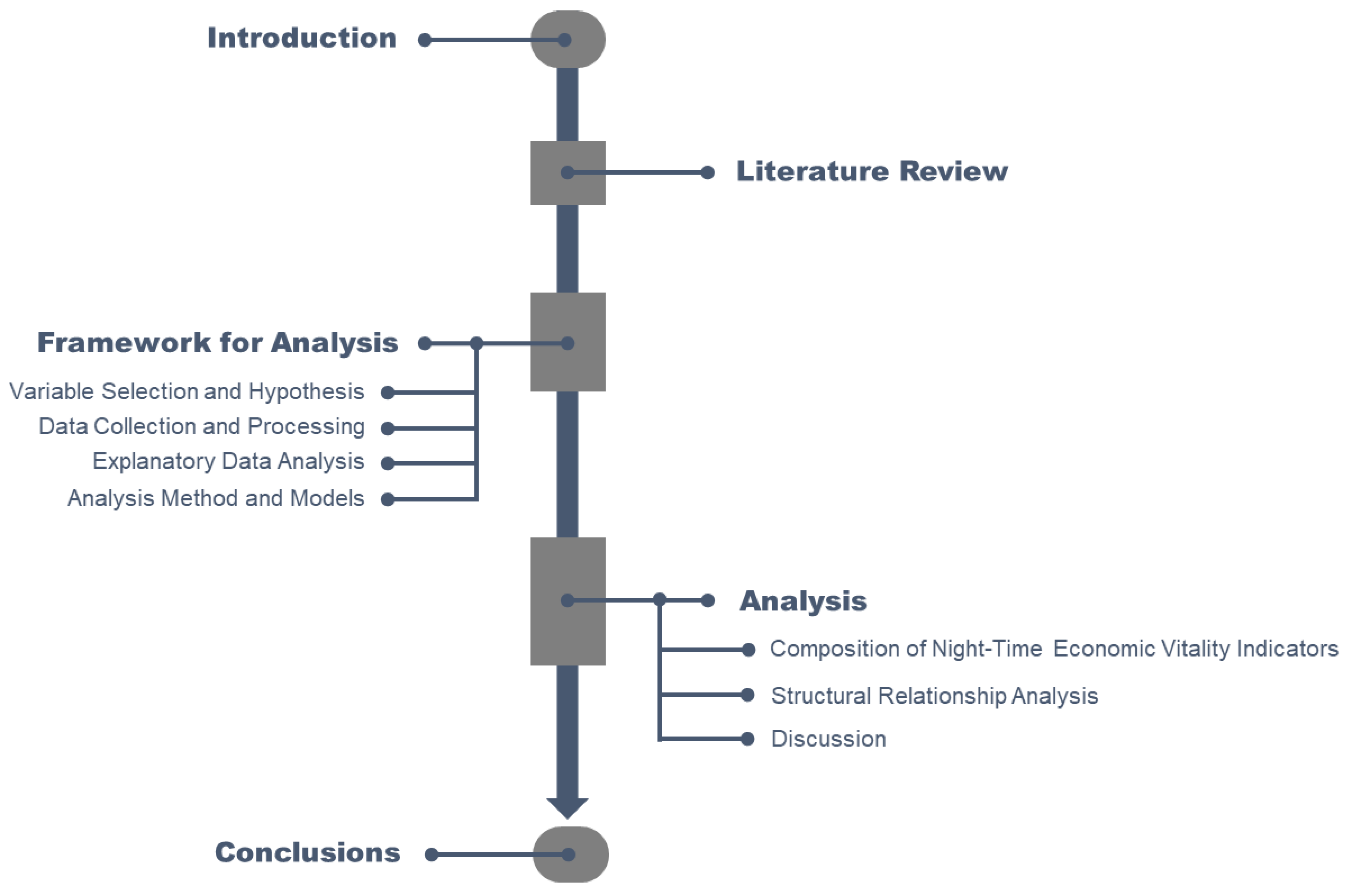
3. Analysis Framework

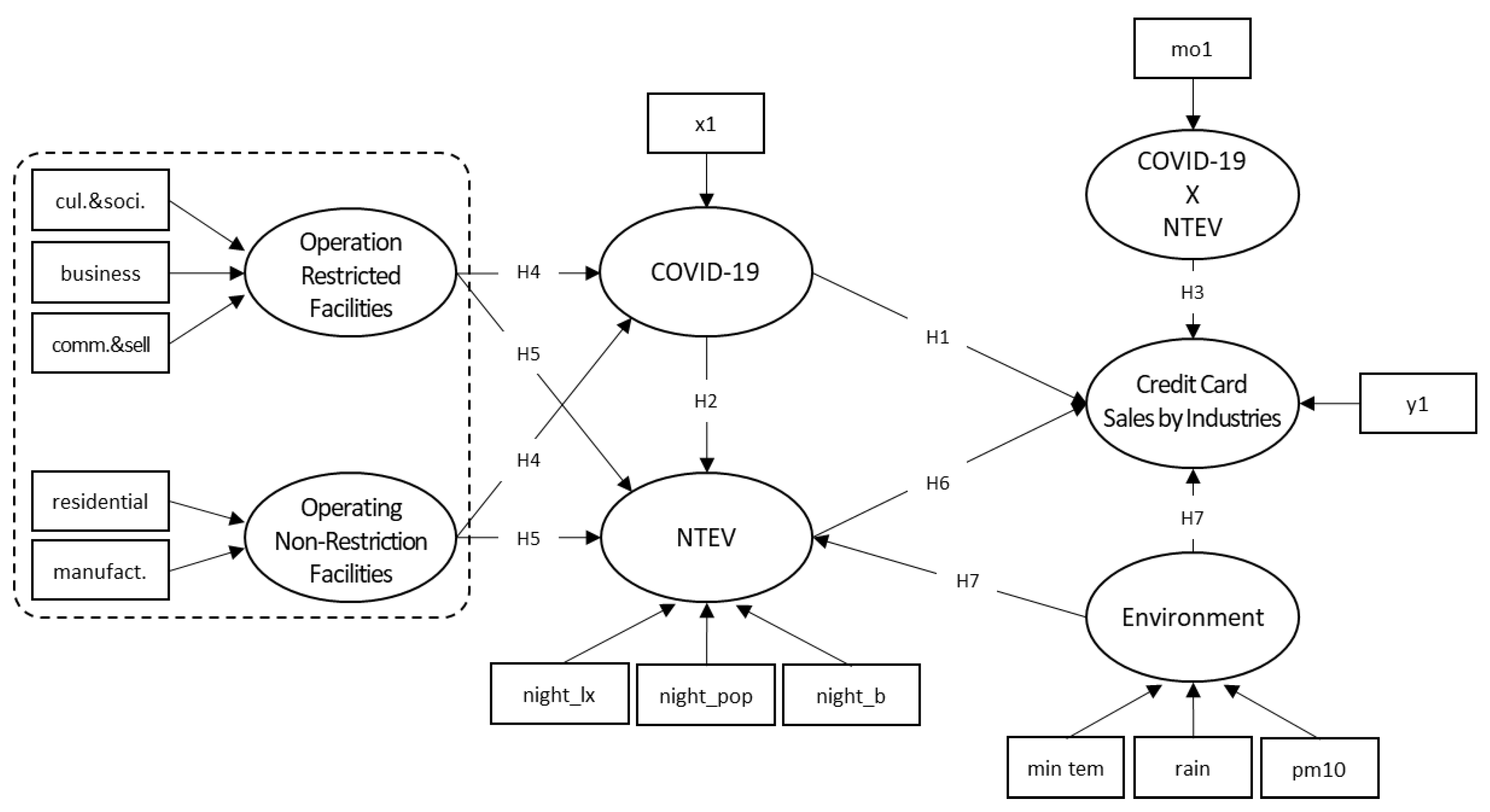
3.1. Variable Selection and Hypothesis

The measures and latent variables required for the analysis were constructed with reference to the literature (Table 1) and used to establish hypotheses. First, to confirm the effect of COVID-19, the COVID-19 construct was devised using the number of daily confirmed patients as a measurement variable.

We constructed the measurement variables of the NTEV by referring to studies such as those of Zikiriya et al., Xia et al., and Jeong and Jun [42,43,44]. Notably, Lin et al. used the nighttime electricity consumption, number of facilities, and online review data as NTEV measurement indicators [5]. Zikiriya et al. identified the urban vitality in the COVID-19 era considering the night-lighting data obtained using satellites [42]. Xia et al. and Jeong and Jun used the number of restaurants and night-lighting data as measures of floating population and credit-card sales, respectively [43,44].

The electricity consumption data for Korea in the night timeslot are not available because they are not segregated by the time zone. Consequently, we used night-lighting data instead of the electricity consumption variable, as an NTEV-related variable. In terms of operating-hour restrictions in response to COVID-19, the Seoul Metropolitan Government designated high-density entertainment facilities as Group 1 and has been managing them stringently. In other words, entertainment facilities, which are the most active at night in Seoul, have been the most adversely affected by COVID-19. In addition, because restaurants and businesses, which have been the focus of existing studies, mainly operate starting from daytime, we selected the number of entertainment facilities such as liquor and karaoke bars (entertainment facilities in Korea are stores that cook and sell food and alcoholic beverages, and they operate only at night) as a variable. Eventually, we used the night-lighting data, number of entertainment facilities, and nightly floating population as measurement indices constituting the NTEV.

To identify the structural relationship between COVID-19, NTEV, and credit-card sales, we considered credit-card sales as the dependent variable, with reference to the literature [5,45,46]. The reason is that credit cards represent the main payment option in many countries [47], and in Korea, the proportion (58.3%) of credit-card payments is higher than that of cash payments (21.6%). Moreover, in recent years, the number of cashless stores in Korea has increased [48]. Furthermore, in this study, the industry of credit-card sales was classified with reference to an existing study [45] that highlighted that the effect of COVID-19 on credit-card sales varied across industries. According to a classification provided by Shinhan Card Co., Ltd. (Seoul, Korea), these industries can be divided into 13 categories: restaurant and entertainment; distribution; food and beverage; clothing and merchandise; sports, culture, and leisure; travel and accommodations; beauty; life service; education and academy; medical care; furniture and home appliances; automobiles; and refueling industries. The furniture and home appliances and automobile industries, which are mainly sales-driven, are merged to obtain 12 categories. The differences across these 12 industrial groups are compared (Table 2).

Given this background, we aimed to evaluate the relationship between the number of confirmed COVID-19 patients and credit-card sales by industry. The influence of the number of confirmed COVID-19 patients on the decrease in self-employment sales has been widely discussed politically and academically [8,45,46], and thus, we established hypothesis Hypothesis 1. We established Hypothesis 2 to examine whether the number of confirmed COVID-19 patients negatively (−) affects the NTEV and Hypothesis 3 to evaluate whether the relationship between the NTEV and credit-card sales is affected by the number of confirmed COVID-19 patients as a moderating variable. Through these hypotheses, we attempted to identify the impact pathway of the number of confirmed COVID-19 patients, that is, direct, indirect, or moderating impact.

Hypothesis 1 (H1).

The number of confirmed COVID-19 patients has a negative (−) effect on credit-card sales.

Hypothesis 2 (H2).

The number of confirmed COVID-19 patients has a negative (−) effect on the NTEV.

Hypothesis 3 (H3).

In the relationship between NTEV and credit-card sales, the number of confirmed COVID-19 patients serves as a moderating variable.

The Seoul Metropolitan Government has implemented a social-distancing policy as a measure to reduce the spread of COVID-19. This policy has been applied differentially to each facility. This objective is to prevent people from being active during night hours and encourage them to return home by limiting the operating hours of commercial facilities to 9 p.m. or 10 p.m. In addition, the Seoul Metropolitan Government has adjusted the number of spectators and events at cultural and sports facilities and recommended or mandated telecommuting for business facilities [49]. Notably, factory facilities related to the manufacturing industry, and residential facilities, have been excluded from these policies. Consequently, the effect relationships of COVID-19 and the NTEV differ depending on the region in which these facilities are concentrated. Because Korea’s COVID-19 policy restricts the use of facilities, several studies have reported that the number of confirmed COVID-19 patients and sales decreased in areas with a high concentration of business and commercial facilities, but increased in areas with a high concentration of residential facilities [50,51]. In addition, because people’s activities have revolved around residential areas after the COVID-19 outbreak, the movements and sizes of floating populations in residential areas have been more intense and larger, respectively, than those in other areas [50,51]. Therefore, to confirm the differences in terms of the density of facilities, we considered the density of each type of facility (residential, manufacturing, cultural, business, and commercial) as measurement variables and categorized them as (1) residential and manufacturing facilities and (2) cultural, business, and commercial facilities. This categorization was performed because Korea has restricted the operations of cultural, business, and commercial facilities under the regulatory policy in response to the pandemic, but the operations of residential and manufacturing facilities have not been restricted. Therefore, we classified the latent variables of the measurement variables as operationally restricted facilities and non-restricted facilities. Hypothesis 4 was established to examine the variation in the effect of the number of confirmed COVID-19 patients in the case of operationally restricted or non-restricted facilities (Hypothesis 4). Thereafter, we investigated whether credit-card sales (Hypothesis 4 + Hypothesis 1) and NTEV (Hypothesis 4 + Hypothesis 2) change with the number of confirmed COVID-19 patients in operationally restricted or non-restricted facilities, through mediation channels.

Hypothesis 4 (H4).

The impact of the number of confirmed COVID-19 patients varies depending on whether the operation of a facility is restricted.

These hypotheses were focused on identifying the effects of the number of confirmed COVID-19 patients. To identify whether the spread of the pandemic influenced the considered structural relationship, the differences among the scenarios were compared by adding a structural relationship that excluded the number of confirmed COVID-19 patients. To this end, we attempted to identify the structural relationship related to COVID-19 from various viewpoints by checking for differences depending on the operating hours of operational restrictions on facilities, even in the absence of confirmed COVID-19 patients (Hypotheses 5 and 6).

Hypothesis 5 (H5).

The impact of the NTEV varies depending on whether the operation of a facility is restricted.

Hypothesis 6 (H6).

The NTEV has a positive (+) impact on credit-card sales.

To effectively examine the abovementioned structural relationship, we set the environmental factors as control variables (Hypothesis 7). Environmental factors that influence the population activity, urban vitality, and credit-card sales include measurement variables such as the minimum temperature, precipitation, and PM₁₀ (Particle Matter 10 μm), as outlined by Yan et al., Keiser et al., and Kang et al. [52,53,54]. Finally, we established Hypothesis 8 to recognize that all of the previous influencing relationships differ by industry [45].

Hypothesis 7 (H7).

In the relationship between the NTEV, COVID-19, and credit-card sales, environmental factors serve as control variables.

Hypothesis 8 (H8).

The structural relationship between the NTEV, COVID-19, and credit-card sales differs by industry.

Table 1. Variables used in previous studies.

Variables			(1)	(2)	(3)	(4)	(5)	(6)	(7)	(8)	(9)	(10)	(11)	This Study
Dependent Variables	Credit-Card Sales	Credit-Card Sales by Industry					●	●	●	●			●	●
Independent Variables	Night Time Economic Vitality	Nighttime Electricity Consumption	●
		Night-Lighting	●	●	●		●							●
		Nightly Floating Population					●				●	●	●	●
		Number of Restaurants			●
		Number of Entertainment Facilities				●								●
		Number of Facilities	●									●
	COVID-19	Number of Confirmed Patients		●					●			●		●
	Operating Restriction/Non-Restricting Facilities	Residential Facilities										●	●	●
		Cultural Facilities												●
		Manufacturing Facilities												●
		Business Facilities										●	●	●
		Commercial Facilities										●	●	●
Control Variables	Environment	Minimum Temperature								●	●			●
		Precipitation								●	●			●
		PM₁₀								●	●			●
		PM₂₅									●

(1) Lin et al., 2021 [5]; (2) Zikiriya et al., 2021 [42]; (3) Xia et al., 2020 [43]; (4) Hobbs et al., 2000 [19]; (5) Jeong and Jun, 2020 [44]; (6) Horvath et al., 2021 [46]; (7) Jo et al., 2020 [45]; (8) Kang et al., 2019 [54]; (9) Yan et al., 2019 [52]; (10) Kim., 2021 [50]; (11) Lim and Choi., 2022 [51].

Table 1. Variables used in previous studies.

Variables			(1)	(2)	(3)	(4)	(5)	(6)	(7)	(8)	(9)	(10)	(11)	This Study
Dependent Variables	Credit-Card Sales	Credit-Card Sales by Industry					●	●	●	●			●	●
Independent Variables	Night Time Economic Vitality	Nighttime Electricity Consumption	●
		Night-Lighting	●	●	●		●							●
		Nightly Floating Population					●				●	●	●	●
		Number of Restaurants			●
		Number of Entertainment Facilities				●								●
		Number of Facilities	●									●
	COVID-19	Number of Confirmed Patients		●					●			●		●
	Operating Restriction/Non-Restricting Facilities	Residential Facilities										●	●	●
		Cultural Facilities												●
		Manufacturing Facilities												●
		Business Facilities										●	●	●
		Commercial Facilities										●	●	●
Control Variables	Environment	Minimum Temperature								●	●			●
		Precipitation								●	●			●
		PM₁₀								●	●			●
		PM₂₅									●

(1) Lin et al., 2021 [5]; (2) Zikiriya et al., 2021 [42]; (3) Xia et al., 2020 [43]; (4) Hobbs et al., 2000 [19]; (5) Jeong and Jun, 2020 [44]; (6) Horvath et al., 2021 [46]; (7) Jo et al., 2020 [45]; (8) Kang et al., 2019 [54]; (9) Yan et al., 2019 [52]; (10) Kim., 2021 [50]; (11) Lim and Choi., 2022 [51].

Table 2. Industry classification of Shinhan Card Co., Ltd., and this study.

Industry Classification of Shinhan Card Co., Ltd.		Facilities Included in the Industry	Industry Classification of This Study
1	Restaurant and Entertainment	e.g., Fast food chain; Cafe; Bakery shop	1	restaurant and entertainment
2	Distribution	e.g., Department store; Convenience store; Market	2	distribution
3	Food and Beverage	e.g., Butcher shop; Fisheries wholesale market; Flower market	3	food and beverage
4	Clothing and Merchandise	e.g., Optician; Jewelry shop; Offline fashion store	4	clothing and merchandise
5	Sports, Culture and Leisure	e.g., Movie theater; Indoor swimming pool; Bookstore	5	Sports, culture and leisure
6	Travel and Accommodations	e.g., Hotel; Duty free shop	6	travel and accommodations
7	Beauty	e.g., Hair shop; Cosmetics store	7	beauty
8	Life service	e.g., Laundry; Shoe repair shop	8	life service
9	Education and Academy	e.g., Reading room; Educational institute; English academy	9	education and academy
10	Medical care	e.g., Hospital; Pharmacy	10	medical care
11	Furniture and Home appliances	e.g., Home appliance store	11	Furniture, home appliances and automobiles
12	Automobiles	e.g., Automobile dealership; Tire sales department
13	Refueling	e.g., Gas station	12	refueling

Table 2. Industry classification of Shinhan Card Co., Ltd., and this study.

Industry Classification of Shinhan Card Co., Ltd.		Facilities Included in the Industry	Industry Classification of This Study
1	Restaurant and Entertainment	e.g., Fast food chain; Cafe; Bakery shop	1	restaurant and entertainment
2	Distribution	e.g., Department store; Convenience store; Market	2	distribution
3	Food and Beverage	e.g., Butcher shop; Fisheries wholesale market; Flower market	3	food and beverage
4	Clothing and Merchandise	e.g., Optician; Jewelry shop; Offline fashion store	4	clothing and merchandise
5	Sports, Culture and Leisure	e.g., Movie theater; Indoor swimming pool; Bookstore	5	Sports, culture and leisure
6	Travel and Accommodations	e.g., Hotel; Duty free shop	6	travel and accommodations
7	Beauty	e.g., Hair shop; Cosmetics store	7	beauty
8	Life service	e.g., Laundry; Shoe repair shop	8	life service
9	Education and Academy	e.g., Reading room; Educational institute; English academy	9	education and academy
10	Medical care	e.g., Hospital; Pharmacy	10	medical care
11	Furniture and Home appliances	e.g., Home appliance store	11	Furniture, home appliances and automobiles
12	Automobiles	e.g., Automobile dealership; Tire sales department
13	Refueling	e.g., Gas station	12	refueling

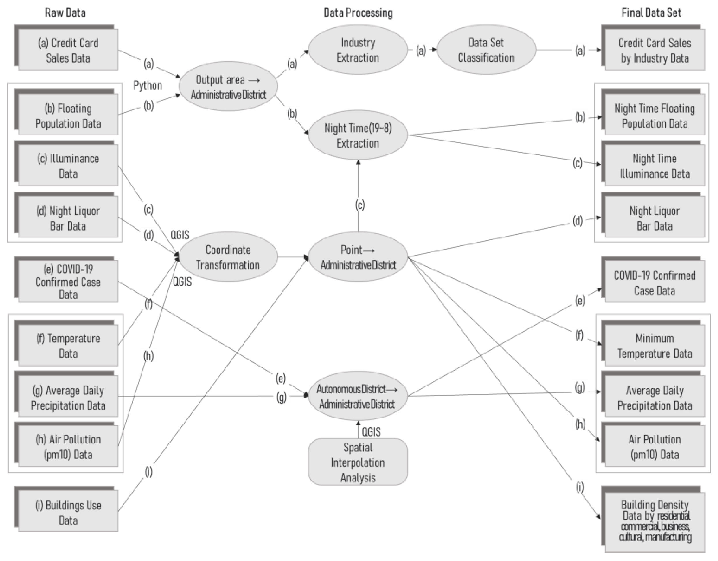
3.2. Data Collection and Processing

The spatial units for data collection were 424 administrative districts (dong) in Seoul. In July 2021, the Seoul Metropolitan Government changed the number of administrative districts to 425, but data for only 424 administrative districts are available. Therefore, we analyzed 424 districts. In terms of the spatial scale of the analysis units, the average area per administrative district was 1.42 km², given that the total area of Seoul is 605.2 km². The temporal target of this study was 2021, and to perform a cross-sectional analysis, we aggregated and analyzed one-year data.

We used the data of Shinhan Card Company (provided by the Seoul Metropolitan Government) as the credit-card sales data, i.e., the dependent variable. Among the independent variables, the entertainment facility variable representing the NTEV was computed by totaling the number of liquor and karaoke bars in operation as of December 2021. To reflect the floating population variable representing the population activity at nighttime, we used the data provided by the Seoul Metropolitan Government.

The illuminance values collected from the Smart-Seoul Data of Things (S-DoT) network were used as the night-lighting variable representing the nighttime brightness. The S-DoT data are real-time data provided by the Seoul Metropolitan Government for identifying and measuring various urban phenomena. As of December 2021, about 1100 monitoring sensors have been installed evenly throughout the 424 administrative districts of Seoul (Figure 2) [55]. The real-time data represent the actual nighttime brightness as the sensing data measured in minutes. We considered both the size of the nightly floating population and night-lighting values in our analysis by extracting only the data corresponding to the night timeslot (from 7 p.m. to 8 a.m.).

Moreover, we used data pertaining to the daily numbers of confirmed COVID-19 patients in 2021 provided by the Korea Centers for Disease Control and Prevention as the COVID-19 variable. Because these data are provided in units of 25 autonomous regions (gu), we requested each autonomous region to provide data in units of 424 administrative districts, which are the unit of analysis of this study (A gu is subdivided into several dong). Only 7 of 25 autonomous regions of Seoul provided the requested data. Therefore, to ensure data consistency, we estimated the data of the administrative district units by using the daily number of confirmed COVID-19 patients provided for the autonomous region units through population interpolation. To ensure the validity of population interpolation and reliability of the estimated data, we verified the accuracy of the population interpolation by comparing the relative errors between the estimated and actual data using the seven datasets of administrative districts units provided by autonomous agencies (Equation (1)). The accuracy of the estimated daily number of confirmed COVID-19 patients by administrative district was 98.96%; therefore, the information was considered useful.

$$\begin{gathered} \mathrm{Accuracy}(\%)=100-\mathrm{elative}\mathrm{Error} \\ \mathrm{Relative}\mathrm{Error}(\%)=\left(\left|\mathsf{ϵ}\right|\right)/\mathrm{X}\times 100 \end{gathered}$$

(1)

The residential, manufacturing, cultural, business, and commercial facility variables, which were classified as operationally restricted and non-restricted facilities, were represented by Seoul’s building data by use type, provided by the Ministry of Land. Notably, these data are point data, and all building data in Seoul are provided in the shp format. Therefore, we used the QGIS (Quantum Geographical Information System version 3.27) online open source program to extract the data provided for each building unit into administrative unit data.

The data of environmental variables can typically be acquired using three approaches: estimation from satellite images; determination using personal measurement means, or measurement using fixed weather-observation equipment [56]. In general, it is challenging to ensure the accuracy of satellite imagery data because of orbital cycles or cloud cover. Landsat data, which have intermediate resolution grades and are suitable for analysis, are often discontinuous because the orbital period is 16 d [57]. In addition, because these data are estimated using the surface radiation energy instead of being directly measured, they may differ marginally from the actual values [58]. Direct data acquisition using personal measurement means is difficult over a large area, which renders it challenging to grasp the trends across the entire city. Moreover, when using the data obtained from fixed weather-observation equipment such as automated weather station (AWS), spatial interpolation must be performed to extract data for a small spatial scale because typically only a few AWS exists in the region. Because the distance between the AWS equipment points is large, the estimated spacing values may differ from the actual values [58]. Considering these aspects, the actual S-DoT data of the minimum temperature and PM₁₀ variables were used in this study. Because S-DoT does not provide precipitation data, the AWS data provided by the Korea Meteorological Administration for each autonomous district were collected, and the average daily rainfall in each administrative dong was estimated through spatial interpolation.

The credit-card sales, nightly floating population, night-lighting data, minimum temperature, and PM₁₀ data, as variables used in this study, represented vast amounts of big data provided temporally. The credit-card sales data were provided on a daily basis for the 19,153-census output area, and the nightly floating population data were provided on an hourly basis for 424 administrative districts. The night-lighting data, minimum temperature, and PM₁₀ data were collected in real time on an hourly basis using about 1100 sensors. Because each dataset was composed of micro units, data mining was performed by administrative district on a one-year basis, as shown in Figure 3.

In particular, because the night-lighting, minimum temperature, and PM₁₀ data obtained from the S-DoT network was expected to have missing values owing to the characteristics of sensing data, we attempted to eliminate any missing values identified in the data-review process.

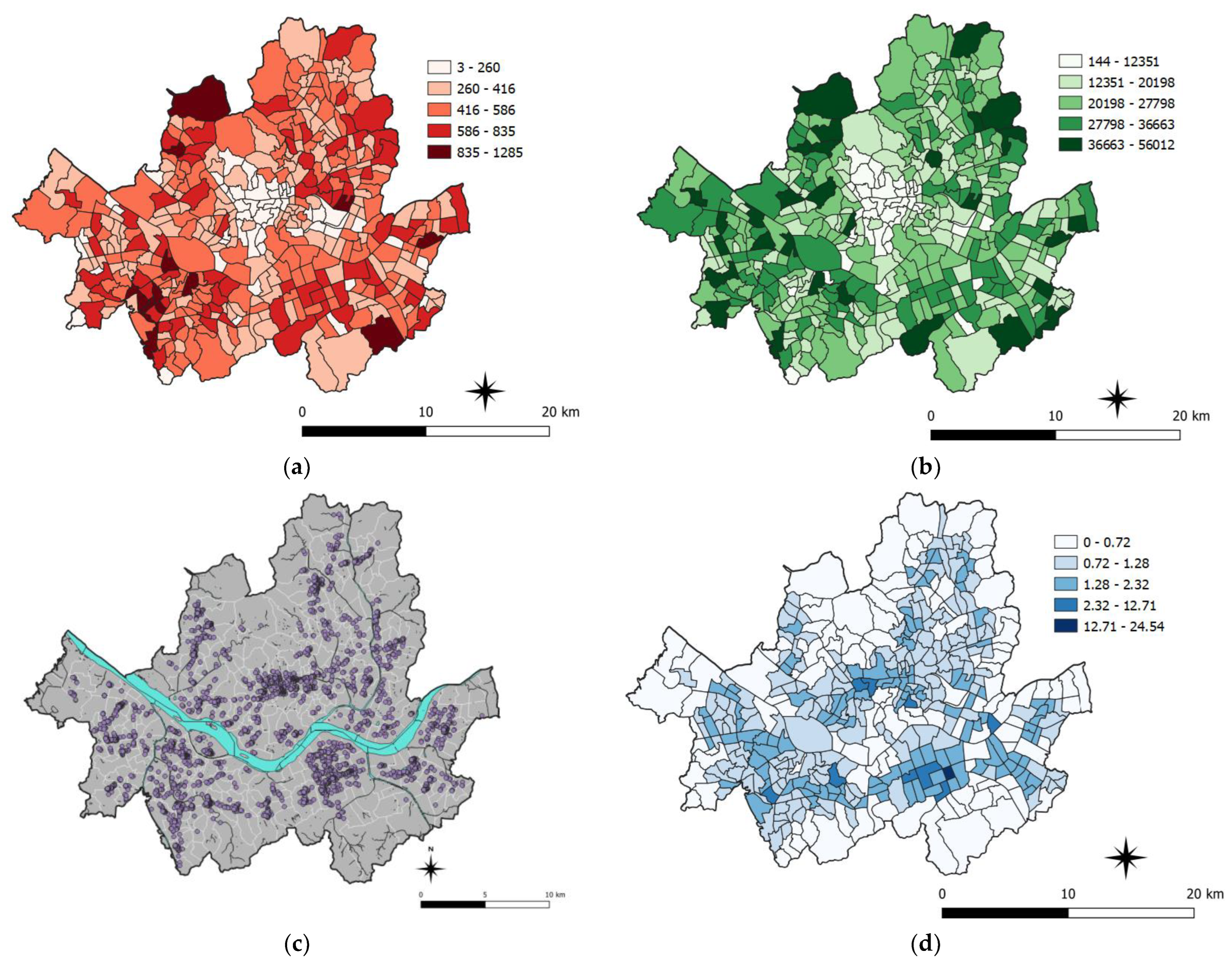
3.3. Explanatory Data Analysis

3.3.1. Descriptive Statistics

Exploratory data analysis was performed to evaluate the accuracy and basic characteristics of the collected data. First, by conducting a descriptive statistics analysis using the SPSS program, the missing values, average values, minimum and maximum values, median values, and kurtosis and skewness of the data were confirmed (

Table 3. Frequency analysis results.

Variables	N	Min	Max.	Avg.	S.D.	Skew.	Kurt.	Variables	N	Min.	Max.	Avg.	S.D.	Skew.	Kurt.
Credit-Card Sales 1: restaurant and entertainment	424	2.9949	88,370.35	2194.54	5996.40	8.80	107.31	Night-Lighting Data	424	0.00	16,019.84	287.60	917.23	14.097	222.741
Credit-Card Sales 2: distribution	423	0.3728	243,033.06	7429.11	26,843.92	6.89	50.85	Nightly Floating Population	424	4327.7196	73,743.06	24,003.87	10,354.77	0.925	1.502
Credit-Card Sales 3: food and beverage	424	0.5145	62,705.36	831.10	3816.55	12.35	178.55	Number of Entertainment Facilities	424	0.00	146.00	9.72	18.78	4.078	20.226
Credit-Card Sales 4: clothing and merchandise	424	0.2229	25,550.11	390.96	1837.39	9.29	103.32	Number of Confirmed Patients	424	2.6635	1285.00	452.21	187.37	0.874	1.741
Credit-Card Sales 5: sports, culture and leisure	424	2.4747	12,255.54	314.65	827.92	9.48	116.91	Residential Facility	424	0.0000	22.76	0.73	1.28	13.907	222.983
Credit-Card Sales 6: travel and accommodation	332	0.0035	79,756.90	1036.87	6566.57	9.77	103.06	Cultural Facility	424	0.0000	0.72	0.09	0.08	3.414	16.915
Credit-Card Sales 7: beauty	424	1.4245	14,536.46	138.53	741.49	17.65	338.72	Manufacturing Facility	424	0.0000	1.83	0.02	0.13	12.891	174.849
Credit-Card Sales 8: life service	424	0.4830	34,616.96	393.62	1820.31	16.11	297.53	Business Facility	424	0.0000	0.09	0.00	0.01	5.452	35.283
Credit-Card Sales 9: education and academy	424	0.9858	39,668.93	893.87	3019.33	7.44	74.16	Commercial Facility	424	0.0000	2.78	0.28	0.33	3.522	18.071
Credit-Card Sales 10: medical care	424	0.5095	108,389.96	2689.10	9548.28	8.21	77.03	Minimum Temperature	424	9.5003	16.44	12.75	0.93	−0.756	1.972
Credit-Card Sales 11: furniture, home appliances and automobiles	424	0.1044	1,149,857.31	3920.09	56,791.39	19.64	394.93	Precipitation	424	0.0308	1.40	0.18	0.18	3.727	18.402
Credit-Card Sales 12: refueling	280	0.6761	68,918.48	8887.12	9596.30	2.32	7.79	PM₁₀	424	0.3668	17.16	2.25	2.15	3.48	16.26

). In addition, data visualization was performed to visually examine the data of major variables such as COVID-19 confirmed cases, floating population, entertainment facilities, and five facility variables. Figure 4 shows the distribution and degree of data for 424 administrative districts in Seoul. The confirmed patients and floating population variables visualized the distribution degree of the population, and the five facility variables integrated all facilities to visualize the density of the entire facility. The number of samples of the entertainment facility variable was smaller than that of the other major variables: there were about 4000, and 101 of the 424 administrative districts of Seoul had zero data because there were no entertainment facilities. Therefore, the location of the entertainment facility variable was confirmed by visualizing the distribution of the facilities.

According to the results, in terms of the credit-card sales by industry, which is a dependent variable, the sample sizes of the distribution, travel and accommodations, and refueling industries differed by 423, 332, and 280, respectively. Therefore, we deleted the three models corresponding to these industries based on the sample size of the industry, not the 424 administrative districts in Seoul. The resulting data were used for the analysis. In addition, we confirmed that the skewness (<3.0) and kurtosis (<7.0) exceeded the criteria, indicating non-normality of the data.

3.3.2. Normality and Preprocessing

Next, we performed quantile-quantile plot (Q-Q plot) and Shapiro–Wilk analysis by using R to confirm the normality of the data and distribution. The results of the Shapiro–Wilk analysis, which confirms the statistical normality, indicated the extremely small p-values of all the variables (

Table 4. Shapiro-Wilk analysis results.

Variables	W	p-Value *	Variables	W	p-Value *
Credit-Card Sales 1: restaurant and entertainment	0.31158	2.2 × 10−16	Night-Lighting Data	0.12087	2.2 × 10−16
Credit-Card Sales 2: distribution	0.23756	2.2 × 10−16	Nightly Floating Population	0.95555	5.303 × 10−10
Credit-Card Sales 3: food and beverage	0.16137	2.2 × 10−16	Number of Entertainment Facilities	0.52375	2.2 × 10−16
Credit-Card Sales 4: clothing and merchandise	0.18961	2.2 × 10−16	Number of Confirmed Patients	0.96143	4.165 × 10−9
Credit-Card Sales 5: sports, culture and leisure	0.29631	2.2 × 10−16	Residential Facility	0.22571	2.2 × 10−16
Credit-Card Sales 6: travel and accommodation	0.14183	2.2 × 10−16	Cultural Facility	0.69550	2.2 × 10−16
Credit-Card Sales 7: beauty	0.10576	2.2 × 10−16	Manufacturing Facility	0.09384	2.2 × 10−16
Credit-Card Sales 8: life service	0.15037	2.2 × 10−16	Business Facility	0.34267	2.2 × 10−16
Credit-Card Sales 9: education and academy	0.28369	2.2 × 10−16	Commercial Facility	0.66494	2.2 × 10−16
Credit-Card Sales 10: medical care	0.25221	2.2 × 10−16	Minimum Temperature	0.93564	1.446 × 10−12
Credit-Card Sales 11: furniture, home appliances and automobiles	0.03860	2.2 × 10−16	Precipitation	0.62332	2.2 × 10−16
Credit-Card Sales 12: refueling	0.77614	2.2 × 10−16	PM₁₀	0.95274	2.107 × 10−10

* The e-value of the p-value means that the p-value is less than or equal to 10 to the power of −n, which indicates an extremely small numerical value that does not satisfy the significance level of >0.05.

) In the scatter plot of each variable in the Q-Q Plot indicated, the data points did not follow a straight line slope, which indicated that the data were not normally distributed (Figure A1).

To convert the units and ranges of different data into forms suitable for analysis and enhance the normality, we performed a normalization process by taking the log of the non-normal data. Thereafter, the abovementioned analysis process was repeated. The results indicated that the range of data was reduced through the use of log, although the normality of certain data did not increase (Figure A1). Thus, the exploratory data analysis indicated that the dataset used in this study did not follow the normal distribution.

3.4. Analysis Method and Models

We performed structural equation modeling (SEM) to clarify the relationship between COVID-19, NTEV, and credit-card sales, which has not been academically identified yet. SEM is a statistical technique designed to analyze structural relationships between correlation and theoretical causality among constituent concepts on the basis of metrics [59]. Because latent factors without measurement errors can be identified through confirmatory factor analysis, and the latent factor relationship can be simultaneously confirmed by a path analysis, the degree of explanation of a research model can be confirmed. This method is mainly used in exploratory studies to analyze multiple influences by simultaneously setting various independent and dependent variables or to identify the direct and indirect effects between the variables [59]. Notably, this method can enhance the analysis reliability by measuring the overall model fit, and handling data that are difficult to calculate (e.g., time-series data with autocorrelation errors, nonnormal distributions, and categorical variables).

According to the results of the exploratory data analysis, the dataset used in this study did not satisfy the conditions of the general structural equation from the standard viewpoint of distribution normality. The general structural equation pertains to covariance-based SEM (CB-SEM), as in the data used in CB-SEM, each variable must represent stationarity as a basic condition [60]. Considering this aspect, we performed PLS-SEM to address the nonnormal data encountered in SEM. The principal-component-based PLS-SEM method is less rigid in terms of the sample size and residual distribution requirements and is, thus, advantageous for analyzing data that do not follow a normal distribution [61]. Moreover, this method can be used to estimate the parameters more efficiently than typical CB-SEMs and offers higher statistical power [62]. In particular, in the application of formative indicators such as urban data to the model, model identification is facile, and the analysis is stable.

PLS-SEM was performed using the Smart-PLS 3.0 program. Figure 5 shows the structural relationship obtained in this study using the PLS-SEM method, and using the example of one of several industry-specific analysis models employed in this study.

The analysis models were composed of the potential variables representing the concept (internal variables) and measurement variables explaining the potential variables (external variables). The measurement of the relationship between these variables was set as the formative measurement model. A key consideration in PLS-SEM is the identification of the measurement indicators, including formative and reflective indicators. The formative indicators are causative indicators, i.e., they define the characteristics of the concept. In addition, a measurement variable induces a latent variable; homogeneity (correlation) between the measurement variables is low, and; these variables are mainly used in relationships in which an effect occurs when one measurement variable is removed. In contrast, reflective indicators are result indicators, i.e., the causal direction is directed from the concept to the indicator, and these indicators are signs of the construct. In other words, latent variables not only induce the measurement variables, but also stipulate that the measurement variables must be similar, such as survey questions [62].

The existing SEM studies mainly used reflective indicators owing to the lack of support for programs that analyze formative indicators or the difficulty associated with identifying models by using formative indicators. In addition, in the data or research to which formative indicators must be applied, reflective indicators have typically been applied. Notably, if the measurement indicators are set incorrectly in the SEM framework, model errors may occur, because the path coefficient and R² increase [59,61]. All the measurement variables used in this study were continuous variables based on urban data, and because the characteristics between the variables were independent, formative indicators were found to be more suitable than reflective indicators. Therefore, considering the data used in this study and objectives, we perform PLS-SEM using a formative measurement model and used all indicators as formative indicators.

In addition, to confirm the effects of the number of confirmed COVID-19 patients from various perspectives, we set the COVID-19-related construct as an exogenous latent variable, an endogenous latent variable, and a moderating variable. In PLS-SEM, because the moderating effect is confirmed as an interaction term, we added a moderating structure by performing mean-centering over the COVID-19 variable. This structural relationship is illustrated in Figure 4. Moreover, to identify the mediation effect of NTEV, we set the NTEV-related construct as an endogenous potential variable, which serves as both an independent variable and a dependent variable.

After setting up the basic study model, we classified and analyzed the analysis model for 12 industries: restaurant and entertainment; distribution; food and beverage; clothing and merchandise; sports, culture, and leisure; travel and accommodation; beauty; life service; education and academy; medical care; furniture, home appliances and automobiles, and; refueling.

When using a formative measurement model, the PLS-SEM analysis process is different from that of CB-SEM or reflective measurement modeling. Because the formative measurement model is free from measurement errors, the measurement variables must be independent and not correlated. Moreover, it is assumed that no error exists between the variables owing to the model characteristics [63,64]. In this context, the formative measurement model has criteria other than the assessment criteria, such as the validity, construct reliability and averaged variance extracted, used in general SEM (or reflective measurement models). As shown in Figure 6, the assessment procedure of the formative measurement model involves verification of the hypothesis of the structural model through path analysis after evaluating the measurement model in terms of the indicator validity, construct validity, outer weight, and outer loading. Therefore, using the Smart-PLS 3.0 program, we constructed the NTEV indicators and analyzed the structural relationships following the procedure of the formative measurement model (Figure 6).

4. Analysis

4.1. Composition of NTEV Indicators

The Smart-PLS program was used to verify the NTEV indicators, as an objective of this study. All the variables used to identify the NTEV, i.e., the nightly floating population, night-lighting, and number of entertainment facilities, were set as indicators based on a review of the existing studies and established theories. The indicators were formative indicators with independent characteristics based on urban data. We performed a rigorous analysis to confirm the significance and suitability of these formative indicators and determine whether they appropriately reflect the construct.

Formative indicators can typically be assessed using the outer weights and outer loadings in bootstrapping analysis. If the t-value of the outer weights is greater than at least ±1.65 at the 10% significance level in the two-tail test, or if the p-value is significant, indicator construction is considered to be possible. In contrast, if the value of the outer weights is not significant, the value of the outer loading must be 0.5 or higher. If the outer weight of an indicator is not significant, and the value of the outer loading is 0.5 or lower, the indicator is not suitable for forming a concept and must be discarded.

Therefore, we performed a bootstrapping analysis involving 5000 extractions to reduce errors and ensure consistency in estimation. In terms of the outer weights, both the t- and p-values were significant (

Table 5. Verification of NTEV indicators (outer weights).

Construct	Indicators	Outer Weights	T-Value	p-Value
NTEV	Nightly Floating Population	0.588	24.002	0.000
	Nightly-Lighting	0.535	13.452	0.000
	Number of Entertainment Facilities	0.306	3.374	0.001

), and the nightly floating population, night-lighting, and number of entertainment facilities were found to be suitable NTEV indicators, even without checking the outer loadings (Table 5).

4.2. Structural Relationship Analysis

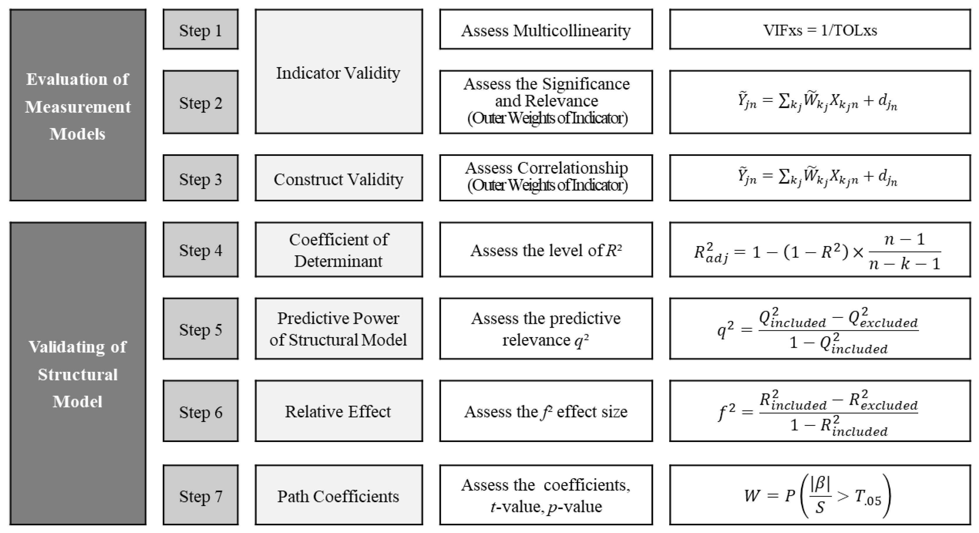
4.2.1. Evaluation of Measurement Models

To evaluate a formative measurement model using formative indicators, the validity of the measurement indicators and constituent factors of the model must be evaluated. In a formative measurement model, both the indicators and constituent factors must be independent and noncorrelated, because strong correlations are problematic from the viewpoints of methodology and interpretation [62,63].

The validity between measurement indicators is typically evaluated considering the multicollinearity, outer weights, and outer loadings. First, in terms of the multicollinearity, the variance inflation factor (VIF), defined as VIFxs = 1/TOLxs, must be 5.0 or less. According to a few researchers, the VIF must be equal to or less than 10, as in case of the reflective indicators, but it is not appropriate to apply the same acceptable reference values to reflective and formative indicators [65,66]. Because all the analysis models used in this study were formative measurement models that used formative indicators, we performed multicollinearity analysis with VIF = 5.0. For all the formative indicators (measurement indicators) constituting the 12 models, the VIF value ranged between 1.000 and 1.145, which indicated the lack of collinearity between the indicators. Thereafter, we analyzed the outer weights or outer loadings to evaluate the contributions and relevance of the formative indicators. This analysis was similar to the process of evaluating the construct validity of the NTEV indicators. The difference was that the previous measurement indicated the validity of the indicators constituting the NTEV concept, whereas this analysis was aimed at confirming the suitability of all indicators constituting the model. The suitability of the indicators reflected whether the corresponding construct of the multiple formative indicators (measurement indicators) was appropriate; thus, single formative indicators, such as the number of confirmed COVID-19 patients and credit-card sales, were not measured.

First, all the 12 models were checked using outer weights to verify the existence of the relative contributions of the formative indicators to the construct, that is, the relative importance levels of the constructs. For all the models, the PM₁₀ variable of the environmental construct, manufacturing variable classified under the non-restricted facilities construct, commercial and business variables classified under the restricted facilities construct, and entertainment facilities variable of the NTEV construct were found to be not significant. If the values of the outer loadings were less than the reference value (0.5) and simultaneously nonsignificant, the indicator was required to be removed. We examined the absolute contribution of the indicators based on the outer loading values. The cultural variables classified under the restricted facility construct were not eliminated because the outer loading values were greater than 0.5 or significant. In particular, although these indicators were insignificant, they were important for the model validity [62]. We eliminated the PM₁₀ variable under the environment construct, manufacturing variable under the non-restricted facilities construct, and business variable under the restricted facilities construct because they were nonsignificant and the value of the outer loadings was less than 0.5.

The outer weight values of the minimum temperature and precipitation variables under the environment construct and night-lighting data and entertainment facilities variables under the NTEV construct were insignificant in several models. According to the outer loadings, all variables except the minimum temperature variable of Model 6 were derived reasonably and were not removed. For the minimum temperature variable, the outer weights and outer loadings were insignificant, but this variable was not removed to ensure model consistency because it was an important indicator and was appropriately derived in several models simultaneously. The VIF values and outer weights values of the final indicators used in this study are summarized in

Table 6. Indicator validity results.

Constructs	Indicators	VIF	Model1	Model2	Model3	Model4	Model5	Model6	Model7	Model8	Model9	Model10	Model11	Model12
			Outer Weights	Outer Weights	Outer Weights	Outer Weights	Outer Weights	Outer Weights	Outer Weights	Outer Weights	Outer Weights	Outer Weights	Outer Weights	Outer Weights
Credit-Card Sales	Sales 1	1.000	1
	Sales 2	1.000	-	1	-	-	-	-	-	-	-	-	-	-
	Sales 3	1.000	-	-	1	-	-	-	-	-	-	-	-	-
	Sales 4	1.000	-	-	-	1	-	-	-	-	-	-	-	-
	Sales 5	1.000	-	-	-	-	1	-	-	-	-	-	-	-
	Sales 6	1.000	-	-	-	-	-	1	-	-	-	-	-	-
	Sales 7	1.000	-	-	-	-	-	-	1	-	-	-	-	-
	Sales 8	1.000	-	-	-	-	-	-	-	1	-	-	-	-
	Sales 9	1.000	-	-	-	-	-	-	-	-	1	-	-	-
	Sales 10	1.000	-	-	-	-	-	-	-	-	-	1	-	-
	Sales 11	1.000	-	-	-	-	-	-	-	-	-	-	1	-
	Sales 12	1.000	-	-	-	-	-	-	-	-	-	-	-	1
NTEV	lux	1.145	0.250 (1.322)	0.000	0.207 (1.333)	0.351 (1.287)	0.569 (**)	0.740 (0.834)	0.055	0.508 (1.555)	0.180 (1.462)	0.340 (1.562)	0.374 (1.484)	0.284 (0.589)
	pop	1.117	0.000	0.009	0.000	0.000	0.000	0.000	0.000	0.000	0.000	0.000	0.000	0.000
	enter	1.027	0.000	0.028	0.139 (***)	0.000	0.000	0.000	0.000	0.000	0.152 (***)	0.000	0.000	0.434 (**)
COVID-19	covid	1.000	1	1	1	1	1	1	1	1	1	1	1	1
Restriction Facility	residential	1.013	1	1	1	1	1	1	1	1	1	1	1	1
Non-Restriction Facility	cultural	1.131	0.087 (**)	0.392 (***)	0.307 (***)	0.721 (**)	0.941 (**)	0.332 (*)	0.806 (**)	0.953 (**)	0.329 (***)	0.805 (**)	0.948 (**)	0.928 (1.080)
	commercial	1.131	0.000	0.04	0.020	0.000	0.000	0.000	0.000	0.000	0.021	0.000	0.000	0.079
Environment	min.tem	1.116	0.000	0.004	0.004	0.001	0.017	0.244 (-)	0.007	0.001	0.256 (0.635)	0.074	0.012	0.825 (0.644)
	precipi.	1.116	0.000	0.000	0.000	0.000	0.000	0.113(1.484)	0.000	0.000	0.009	0.014	0.000	0.286 (1.053)

( ) denotes the outer loading value of the nonsignificant indicator from outer weights. If the outer weights do not satisfy the condition, the outer loadings must satisfy either the coefficient value or the significance value. Coefficient values greater than or equal to 0.5 are indicated by numerical values, and the significant values are indicated by *, **, ***.

.

Subsequently, we confirmed the validity between the constructs. For the formative measurement model, the correlation between all constructs must be less than 0.7 [67]. According to the analysis results, the relationship between the constructs was less than 0.7 for all models, which confirmed that the constructs composed of the formative indicators were independent of one another.

4.2.2. Structural Model Validation

Before the path analysis, we computed the R² and Q² values to measure the predictive accuracy and suitability, respectively, of the formative measurement model of PLS-SEM. Because the R² value indicates a higher level of prediction accuracy with a larger coefficient, and the standard for an acceptable R² value depends on the model complexity and the study premise, researchers must check the coefficient level of the overall research model, then decide the standard by referring to previous studies. In urban studies, values between 0.02 and 0.12 are considered weak, those between 0.13 and 0.25 are considered moderate, and those higher than 0.26 are considered strong [68]. According to the analysis results, most of the 12 industries exhibited moderate or strong model accuracy, and the COVID-19 construct of Model 6 and COVID-19 and credit-card sales constructs of Model 12 exhibited low accuracies (

Table 7. Coefficients of determination of the models.

Models		R²	Adj. R²	Q²
1	sales	0.548	0.544	0.503
	covid	0.150	0.146	0.093
	night	0.589	0.585	0.246
2	sales	0.367	0.361	0.264
	covid	0.147	0.143	0.087
	night	0.606	0.602	0.241
3	sales	0.301	0.296	0.264
	covid	0.148	0.144	0.089
	night	0.605	0.601	0.239
4	sales	0.387	0.383	0.361
	covid	0.150	0.146	0.094
	night	0.580	0.576	0.244
5	sales	0.498	0.495	0.480
	covid	0.149	0.145	0.093
	night	0.597	0.593	0.247
6	sales	0.354	0.346	0.319
	covid	0.120	0.114	0.100
	night	0.575	0.569	0.229
7	sales	0.508	0.505	0.487
	covid	0.149	0.145	0.092
	night	0.601	0.597	0.247
8	sales	0.369	0.365	0.312
	covid	0.150	0.146	0.093
	night	0.592	0.588	0.245
9	sales	0.284	0.279	0.246
	covid	0.148	0.144	0.089
	night	0.605	0.601	0.239
10	sales	0.403	0.399	0.363
	covid	0.149	0.145	0.092
	night	0.602	0.598	0.248
11	sales	0.274	0.268	0.233
	covid	0.149	0.144	0.093
	night	0.597	0.593	0.246
12	sales	0.037	0.023	−0.004
	covid	0.084	0.077	0.077
	night	0.649	0.644	0.238

). Therefore, we excluded Models 6 and 12 from the path analysis because of their low predictive accuracy.

The Q² value indicates predictive relevance. If the Q² value is 0 or higher, the standard is satisfied. According to the analysis, a negative (−) value was obtained for Model 12, which implied that the model had no predictive relevance (Table 7). For the other 11 models, the path model was noted to be a structurally acceptable measurement model [69].

Because this analysis was aimed at verifying the structural relationship of the models, if the predictive power of a measurement model was low, its reliability of the analysis result was low. Therefore, based on the results of previous analyses (evaluation of measurement models and structural model validation), we selected 10 models for the path analysis, after excluding Models 6 and 12 from the subsequent analysis.

Thereafter, we identified the structural relationships of the 10 industries through a path analysis. The results of hypothesis testing and path analysis conducted using the formative measurement model of PLS-SEM are presented in

Table A1. Path and f² analysis results.

Model 1	Path Coefficients	t Statistics	f²	Hypotheses	Hypotheses Test
COVID → sales	−0.415 ***	5.880	0.179	Hypothesis 1	H₀ Reject
					H₁ Accept
COVID → night	0.645 ***	11.441	0.693	Hypothesis 2	H₀ Accept
					H₁ Reject
COVID * → sales	−0.125	1.525	0.065	Hypothesis 3	H₀ Accept
					H₁ Reject
non-restric. → COVID	0.406 ***	3.389	0.167	Hypothesis 4	H₀ Reject
restric. → COVID	−0.062	0.902	0.004		H₁ Accept
non-restric. → night	−0.283 **	2.882	0.107	Hypothesis 5	H₀ Reject
restric. → night	0.494 ***	7.285	0.505		H₁ Accept
night → sales	0.806 ***	14.085	0.864	Hypothesis 6	H₀ Reject
					H₁ Accept
evir → sales	0.217 ***	5.989	0.095	Hypothesis 7	H₀ Accept
evir → night	0.070	1.210	0.008		H₁ Reject
Model 2	Path Coefficients	t Statistics	f²	Hypotheses	Hypotheses Test
COVID → sales	−0.174 **	1.985	0.016	Hypothesis 1	H₀ Reject
					H₁ Accept
COVID → night	0.730 ***	14.160	0.901	Hypothesis 2	H₀ Accept
					H₁ Reject
COVID * → sales	−0.127 *	1.770	0.053	Hypothesis 3	H₀ Reject
					H₁ Accept
non-restric. → COVID	0.402 ***	3.479	0.153	Hypothesis 4	H₀ Reject
restric. → COVID	−0.047	0.625	0.002		H₁ Accept
non-restric. → night	−0.232 **	2.568	0.069	Hypothesis 5	H₀ Reject
restric. → night	0.313 ***	3.293	0.199		H₁ Accept
night → sales	0.595 ***	7.233	0.252	Hypothesis 6	H₀ Reject
					H₁ Accept
evir → sales	0.110 **	2.498	0.017	Hypothesis 7	H₀ Reject
evir → night	0.100 *	1.768	0.017		H₁ Accept
Model 3	Path Coefficients	t Statistics	f²	Hypotheses	Hypotheses Test
COVID → sales	0.043	0.548	0.001	Hypothesis 1	H₀ Accept
					H₁ Reject
COVID → night	0.723 ***	12.409	0.818	Hypothesis 2	H₀ Accept
					H₁ Reject
COVID * → sales	−0.027	0.576	0.002	Hypothesis 3	H₀ Accept
					H₁ Reject
non-restric. → COVID	0.402 ***	3.501	0.151	Hypothesis 4	H₀ Reject
restric. → COVID	−0.042	0.565	0.002		H₁ Accept
non-restric. → night	−0.205 **	2.050	0.048	Hypothesis 5	H₀ Reject
restric. → night	0.283 **	2.811	0.162		H₁ Accept
night → sales	0.503 ***	7.451	0.159	Hypothesis 6	H₀ Reject
					H₁ Accept
evir → sales	−0.005	0.107	0.000	Hypothesis 7	H₀ Accept
evir → night	0.129	1.319	0.024		H₁ Reject
Model 4	Path Coefficients	t Statistics	f²	Hypotheses	Hypotheses Test
COVID → sales	−0.320 ***	4.483	0.086	Hypothesis 1	H₀ Reject
					H₁ Accept
COVID → night	0.626 ***	10.663	0.658	Hypothesis 2	H₀ Accept
					H₁ Reject
COVID * → sales	−0.068	1.162	0.014	Hypothesis 3	H₀ Accept
					H₁ Reject
non-restric. → COVID	0.405 ***	3.362	0.168	Hypothesis 4	H₀ Reject
restric. → COVID	−0.063	0.946	0.004		H₁ Accept
non-restric. → night	−0.294 **	2.997	0.118	Hypothesis 5	H₀ Reject
restric. → night	0.521 ***	7.175	0.549		H₁ Accept
night → sales	0.713 ***	14.546	0.535	Hypothesis 6	H₀ Reject
					H₁ Accept
evir → sales	0.111 **	2.483	0.019	Hypothesis 7	H₀ Accept
evir → night	0.054	0.888	0.005		H₁ Reject
Model 5	Path Coefficients	t Statistics	f²	Hypotheses	Hypotheses Test
COVID → sales	−0.348 ***	4.829	0.105	Hypothesis 1	H₀ Reject
					H₁ Accept
COVID → night	0.663 ***	11.909	0.706	Hypothesis 2	H₀ Accept
					H₁ Reject
COVID * → sales	−0.058	1.050	0.013	Hypothesis 3	H₀ Accept
					H₁ Reject
non-restric. → COVID	0.406 ***	3.442	0.165	Hypothesis 4	H₀ Reject
restric. → COVID	−0.060	0.845	0.004		H₁ Accept
non-restric. → night	−0.267 **	2.551	0.089	Hypothesis 5	H₀ Reject
restric. → night	0.459 ***	6.568	0.442		H₁ Accept
night → sales	0.835 ***	18.422	0.792	Hypothesis 6	H₀ Reject
					H₁ Accept
evir → sales	0.102 **	2.640	0.019	Hypothesis 7	H₀ Accept
evir → night	0.095	1.423	0.014		H₁ Reject
Model 7	Path Coefficients	t Statistics	f²	Hypotheses	Hypotheses Test
COVID → sales	−0.211 **	3.070	0.037	Hypothesis 1	H₀ Reject
					H₁ Accept
COVID → night	0.695 ***	13.257	0.835	Hypothesis 2	H₀ Accept
					H₁ Reject
COVID * → sales	−0.048	0.856	0.009	Hypothesis 3	H₀ Accept
					H₁ Reject
non-restric. → COVID	0.406 ***	3.404	0.163	Hypothesis 4	H₀ Reject
restric. → COVID	−0.058	0.817	0.003		H₁ Accept
non-restric. → night	−0.279 **	2.885	0.107	Hypothesis 5	H₀ Reject
restric. → night	0.430 ***	6.020	0.384		H₁ Accept
night → sales	0.825 ***	16.955	0.744	Hypothesis 6	H₀ Reject
					H₁ Accept
evir → sales	−0.008	0.170	0.000	Hypothesis 7	H₀ Accept
evir → night	0.070	1.052	0.009		H₁ Reject
Model 8	Path Coefficients	t Statistics	f²	Hypotheses	Hypotheses Test
COVID → sales	−0.351 ***	3.867	0.092	Hypothesis 1	H₀ Reject
					H₁ Accept
COVID → night	0.659 ***	10.808	0.720	Hypothesis 2	H₀ Accept
					H₁ Reject
COVID* → sales	−0.110	1.420	0.037	Hypothesis 3	H₀ Accept
					H₁ Reject
non-restric. → COVID	0.406 ***	3.421	0.166	Hypothesis 4	H₀ Reject
restric. → COVID	−0.061	0.866	0.004		H₁ Accept
non-restric. → night	−0.285 **	2.893	0.107	Hypothesis 5	H₀ Reject
restric. → night	0.479 ***	5.621	0.475		H₁ Accept
night → sales	0.680 ***	10.140	0.445	Hypothesis 6	H₀ Reject
					H₁ Accept
evir → sales	0.191 ***	4.784	0.055	Hypothesis 7	H₀ Accept
evir → night	0.070	1.200	0.008		H₁ Reject
Model 9	Path Coefficients	t Statistics	f²	Hypotheses	Hypotheses Test
COVID → sales	−0.346 ***	4.268	0.055	Hypothesis 1	H₀ Reject
					H₁ Accept
COVID → night	0.721 ***	12.511	0.815	Hypothesis 2	H₀ Accept
					H₁ Reject
COVID * → sales	−0.077	1.433	0.017	Hypothesis 3	H₀ Accept
					H₁ Reject
non-restric. → COVID	0.402 ***	3.527	0.152	Hypothesis 4	H₀ Reject
restric. → COVID	−0.043	0.563	0.002		H₁ Accept
non-restric. → night	−0.207 **	2.079	0.049	Hypothesis 5	H₀ Reject
restric. → night	0.289 **	2.764	0.169		H₁ Accept
night → sales	0.712 ***	11.348	0.316	Hypothesis 6	H₀ Reject
					H₁ Accept
evir → sales	0.012	0.258	0.000	Hypothesis 7	H₀ Accept
evir → night	0.129	1.359	0.023		H₁ Reject
Model 10	Path Coefficients	t Statistics	f²	Hypotheses	Hypotheses Test
COVID → sales	−0.179 **	2.302	0.022	Hypothesis 1	H₀ Reject
					H₁ Accept
COVID → night	0.682 ***	11.759	0.762	Hypothesis 2	H₀ Accept
					H₁ Reject
COVID* → sales	−0.079	1.396	0.021	Hypothesis 3	H₀ Accept
					H₁ Reject
non-restric. → COVID	0.406 ***	3.476	0.163	Hypothesis 4	H₀ Reject
restric. → COVID	−0.058	0.820	0.003		H₁ Accept
non-restric. → night	−0.263 **	2.567	0.087	Hypothesis 5	H₀ Reject
restric. → night	0.429 ***	5.390	0.387		H₁ Accept
night → sales	0.727 ***	12.532	0.482	Hypothesis 6	H₁ Accept
evir → sales	−0.031	0.668	0.002	Hypothesis 7	H₀ Accept
evir → night	0.096	1.107	0.015		H₁ Reject
Model 11	Path Coefficients	t Statistics	f²	Hypotheses	Hypotheses Test
COVID → sales	−0.237 **	2.937	0.034	Hypothesis 1	H₀ Reject
					H₁ Accept
COVID → night	0.670 ***	10.759	0.744	Hypothesis 2	H₀ Accept
					H₁ Reject
COVID* → sales	−0.056	1.360	0.008	Hypothesis 3	H₀ Accept
					H₁ Reject
non-restric. → COVID	0.406 ***	3.447	0.165	Hypothesis 4	H₀ Reject
restric. → COVID	−0.060	0.850	0.004		H₁ Accept
snon-restric. → night	−0.276 **	2.744	0.099	Hypothesis 5	H₀ Reject
restric. → night	0.458 ***	4.906	0.439		H₁ Accept
night → sales	0.596 ***	10.869	0.277	Hypothesis 6	H₀ Reject
					H₁ Accept
evir → sales	0.106 **	2.168	0.014	Hypothesis 7	H₀ Accept
evir → night	0.081	1.217	0.011		H₁ Reject

* p < 0.05, ** p < 0.01, *** p < 0.001

. Table A1 presents the results of not only the alternative hypothesis representing the research hypothesis, but also the null hypothesis and f² value indicating the degree of contribution of the exogenous latent variable to the endogenous latent variable.

The f² value indicates the effect size of the causative variable on the resulting variable. When the effect size is between 0.02 and 0.15, the effect of the exogenous latent variable is small. When the effect size is between 0.15 and 0.35, the exogenous latent variable has a moderate effect on the endogenous latent variable. When the effect size is 0.35 or higher, the exogenous latent variable has a strong effect on the endogenous latent variable. The effect size can be represented as “has” or “does not have” and large or small [69]. According to the analysis results, in the relationships in which the p-value of the path was insignificant, the f² value had no effect or small effect size (Table A1).

As shown in Table A1, we first verified only the hypothesized direct paths. The path analysis results for each hypothesis could be summarized as follows. According to Hypothesis 4, the areas with concentrated operationally non-restricted facilities had a positive (+) effect on the number of confirmed COVID-19 patients, whereas the areas with concentrated operationally restricted facilities did not affect the number of confirmed COVID-19 patients. These results were the same across all 10 models, and the result of Hypothesis 4 could be interpreted as the count of the number of confirmed COVID-19 patients in Korea. Because the number of confirmed COVID-19 patients in Korea was based on resident registration [70], the number of confirmed COVID-19 patients increased in the residential areas, whereas the cultural and commercial areas were not influenced. Therefore, Hypothesis 4, which stated that the effect on the number of confirmed COVID-19 patients differed with the concentration of operationally restricted or non-restricted facilities, was accepted.

Hypotheses 2 and 5 related to night economic vitality were tested. Hypothesis 2, which stated that the number of confirmed COVID-19 patients had a negative (−) effect on the NTEV, was rejected because a positive (+) result was observed for all models. In contrast, Hypothesis 5, which stated that the effect of the model on the NTEV differed depending on whether facilities are operationally restricted or non-restricted, was accepted for all models. Specifically, the results varied across the types of facilities: The operationally non-restricted and restricted facilities had a negative (−) and positive (+) effect on the NTEV, respectively.

The results of Hypotheses 2 and 5 could be interpreted as follows: First, as in the case Hypothesis 5 without a COVID-19 construct, if no pandemic occurred and the facilities were operating in the current state (if the operating hours, number of operations, and number of visitors to the facility were the same as those in the current limited state), the vitality of the night timeslot appeared to be active in areas with concentrated cultural and commercial facilities. Conversely, in residential areas, the vitality of the night timeslot tended to decrease. Moreover, according to Hypothesis 2, more confirmed COVID-19 patients in an area corresponded to a higher nighttime vitality in the area.

These results were more extensively interpreted by examining the mediated paths (restricted/non-restricted facilities → COVID-19 → night in

Table A2. Detailed path analysis results.

Path Coefficients	Model 1	Model 2	Model 3	Model 4	Model 5
non-restric. → night → sales	−0.228	−0.138	−0.103	−0.210	−0.223
restric. → night → sales	0.398	0.186	0.143	0.372	0.383
non-restric. → COVID → sales	−0.168	−0.070	0.017	−0.130	−0.141
restric. → COVID → sales	0.026	0.008	−0.002	0.020	0.021
non-restric. → COVID → night	0.262	0.293	0.290	0.254	0.269
restric. → COVID → night	−0.040	−0.035	−0.031	−0.039	−0.040
COVID → night → sales	0.520	0.434	0.364	0.447	0.553
non-restric. → COVID → night → sales	0.211	0.174	0.146	0.181	0.224
restric. → COVID → night → sales	−0.032	−0.021	−0.015	−0.028	−0.033
Path Coefficients	Model 7	Model 8	Model 9	Model 10	Model 11
non-restric. → night → sales	−0.230	−0.194	−0.147	−0.191	−0.164
restric. → night → sales	0.355	0.326	0.206	0.312	0.273
non-restric. → COVID → sales	−0.086	−0.142	−0.139	−0.073	−0.096
restric. → COVID → sales	0.012	0.021	0.015	0.010	0.014
non-restric. → COVID → night	0.282	0.267	0.290	0.277	0.272
restric. → COVID → night	−0.041	−0.040	−0.031	−0.040	−0.040
COVID → night → sales	0.573	0.448	0.513	0.496	0.400
non-restric. → COVID → night → sales	0.232	0.182	0.206	0.201	0.162
restric. → COVID → night → sales	−0.033	−0.027	−0.022	−0.029	−0.024

). Table A2 shows the results of intermediate or indirect paths. The indirect path reflected the indirect effects between two or more variables through the statistical significance between the paths, although no hypotheses were established for this aspect [62]. Therefore, in addition to the hypotheses representing the direct path, we examined various paths through the indirect path.

In a path without the pandemic (Hypothesis 5), the NTEV was invigorated in areas with concentrated cultural and commercial facilities and suppressed in residential areas. In contrast, in the mediated path with the pandemic, the NTEV was invigorated in areas with concentrated residential facilities and not affected in areas with concentrated cultural and commercial facilities. These results highlighted that when the number of confirmed patients was considered, the scope of people’s activities changed from cultural and commercial facilities to residential facilities. This finding is attributable to the fact that confirmed patients cannot leave the vicinity of their residences under Korea’s COVID-19 regulation policy [70]; thus, people respond sensitively to the number of confirmed patients and reduce the scope of activities near their residences. Consequently, during the pandemic, in residential areas, the number of confirmed patients was high, and simultaneously, the NTEV increased. Moreover, in the areas with concentrated cultural and commercial facilities, no correlation was observed between the number of confirmed patients and NTEV. The result of Hypothesis 2 (COVID-19 had a positive effect on NTEV) could alternatively be interpreted as follows: In both the direct and indirect paths (mediated paths) from the operationally restricted or non-restricted facilities to the NTEV, the coefficient values were larger in the residential areas than those in the cultural and commercial areas, suggesting that the characteristics of the residential areas had a stronger effect on Hypothesis 2.

Hypothesis 1, which stated that the number of confirmed COVID-19 patients negatively (−) affected credit-card sales, was accepted because a negative (−) effect was observed in all nine industries, except the food and beverage industry. In other words, the number of confirmed COVID-19 patients adversely influenced the sales in most industries. In the case of the food and beverage industry, the sales were not affected by the number of confirmed COVID-19 patients because people continued to consume the products, regardless of the pandemic. Furthermore, according to the mediation path (COVID-19 → night → sales in Table A2), even if COVID-19 had an effect, the credit-card sales in all industries increased when using NTEV as the mediation path. These results highlighted that the NTEV factor is important for increasing sales across industries. Upon reconfirming this result based on the direct path between the NTEV and credit-card sales (Hypothesis 6), from which the number of confirmed patients of COVID-19 was removed, it was found that the NTEV had a positive (+) effect on credit-card sales. Thus, Hypothesis 6 was accepted for all models, and we confirmed that the NTEV had a strong positive effect on credit-card sales.

In addition, the paths formed according to the types of facilities were examined. When the COVID-19 factor was removed (restricted/non-restricted facilities → night → sales in Table A2), even when the NTEV was used as a mediated factor, credit-card sales decreased in residential areas but increased in areas with cultural and commercial facilities. When the COVID-19 factor was considered (restricted/non-restricted facilities → covid → night → sales in Table A2), unlike the previous results, credit-card sales increased in residential areas and were unaffected in areas with a concentration of cultural and commercial facilities. Similar to the results of Hypothesis 2 and 5, in the absence of the COVID-19 factor, people’s consumption was centered in areas with a concentration of cultural and commercial facilities. In contrast, in the presence of the COVID-19 factor, people’s consumption was centered in areas with a concentration of residential facilities. These results demonstrated that the scope of not only the activities, but also the consumption changed around residential areas due to COVID-19.

Hypothesis 3, representing the moderating effect, and Hypothesis 7, representing the control effect, were rejected for all models, except the distribution industry. In the formative measurement model of PLS-SEM, the moderating and control effects were interpreted as being present and absent if the path was significant and not significant, respectively. Therefore, Hypothesis 3, which stated that the number of confirmed COVID-19 patients had an effect as a moderating variable on the relationship between the NTEV and credit-card sales, was accepted only in the distribution industry (Model 2) owing to the significant effect in the negative (−) direction. For the remaining nine models, the hypothesis was rejected, confirming that the number of confirmed COVID-19 patients did not have any moderating effect. In addition, the control effect of the environmental factor (Hypothesis 7) appeared to be significantly positive (+) in the distribution industry, indicating that the control effect was present. In contrast, no effect was observed for the other nine models. The significant result obtained for the moderating effect of COVID-19 in the relationship between the NTEV and credit-card sales of the distribution industry indicated that sales decreased because of COVID-19 in typical distribution industries, such as large supermarkets and department stores. Moreover, the significant result obtained for the control effect in the distribution industry indicated that the environmental factors had a positive effect in terms of increasing sales in the distribution industry. This result is consistent with that of a previous study [71], which indicated that the distribution industry was negatively (−) affected by COVID-19 but positively (+) affected by environmental factors, such as temperature and precipitation, compared to other industries.

Finally, because the relationship between the paths was not the same across all the models, Hypothesis 8, which stated that the structural relationship of the models differed according to the industry, was accepted.

4.3. Discussion

According to the path analysis and hypothesis testing using 10 models with 10 indicators for each model, Hypothesis 4, Hypothesis 5, and Hypothesis 6 were accepted for all models, and Hypothesis 2 was rejected for all models. Hypothesis 1 was accepted for all models, except the food and beverage industry, and Hypothesis 3 and Hypothesis 7 were rejected for all models, except the distribution industry. Hypothesis 8 was accepted (the structural relationships differed by industry).

The structural relationship derived in this study can be interpreted as follows (Appendix B and Appendix C): First, the number of confirmed COVID-19 patients changes the scope of people’s activities and consumption spaces. If the impact of COVID-19 is not considered, people’s consumption and nighttime activities are enhanced in areas with a concentration of cultural and commercial facilities compared to those in areas with a concentration of residential facilities. In other words, if the operating hours of commercial facilities are shortened or the number of operations of cultural facilities is reduced (as in the current scenario) and the factor of the number of confirmed COVID-19 patients is absent, people would consume and engage in nighttime activities in areas with a concentration of cultural and commercial facilities. In contrast, if the COVID-19 impact spreads, and the number of confirmed patients increases, people’s consumption and nighttime activity spaces may change from cultural and commercial facilities to residential facilities. These results are consistent with those of several previous studies [50,51] that indicated that people focused their activities in residential areas due to COVID-19.

Second, because of the effect of Korea’s COVID-19 regulation policy, people’s activities are concentrated around residential areas rather than cultural and commercial areas as the effect of COVID-19 intensifies. Korea has restricted the operating hours of cultural and commercial facilities as a part of its COVID-19 policy. Consequently, in the paths in which the number of confirmed COVID-19 patients was included, the activity patterns in the areas with a concentration of cultural and commercial facilities, where operations were restricted, and those in the areas with a concentration of residential facilities, where operations were not restricted, were reversed. These phenomena are attributable to the effect of the COVID-19 policy that limited the scope of people’s activities to areas with a concentration of residential facilities.

Third, the NTEV is a major factor influencing the increase in the sales of various industries. In the direct path between the NTEV and credit-card sales, the NTEV had a positive effect on the credit-card sales. Moreover, in the mediated path between COVID-19, NTEV, and credit-card sales, the NTEV led to increased credit-card sales. In the direct path between COVID-19 and credit-card sales, the latter decreased owing to the number of confirmed patients, but in the indirect path between COVID-19, NTEV, and credit-card sales, the latter increased due to the NTEV input. Therefore, the analysis results of this study support the results of previous studies [5,12,72] that the local economy is vitalized when the local NTEV is activated.

5. Conclusions

The NTE invigorates night consumption markets and vitalizes cities. Therefore, major cities worldwide have taken increased interest in the NTE as a measure to boost urban economies, enhance citizens’ leisure and tourism activities, and revitalize cities that have been affected by COVID-19 [73]. However, the understanding of and interest in the NTE and NTEV in Korea is inadequate. Moreover, NTE-related academic research in Korea has mainly been conducted in the field of tourism studies. In the field of urban studies, only limited research has been performed to measure the urban vitality through nighttime satellite imagery. None of the existing studies on the NTE have reflected the limited operating hours in response to the COVID-19 pandemic.

Therefore, this study has the following academic contributions to Korean research: We attempted to empirically analyze the concept of the NTE, which is being actively studied globally but has not been sufficiently reviewed in Korea. Moreover, we developed quantitative indicators of NTEV for Korea by applying the NTE concept to urban studies, which have otherwise focused mainly on the qualitative indicators used in tourism-related studies. This study is timely, in that, it exploratorily confirms the structural relationship between NTEV, COVID-19, and credit-card sales in Seoul, where the COVID-19 regulation pertaining to operating restrictions was applied the most strictly in Korea.

According to a comparison of the results of this study to those of previous studies, the relationship between NTEV and credit-card sales was identified in the same context as that in the studies of Lin et al. and Fu et al. [5,72]. In other words, we confirmed that the NTEV activates the consumption economy of the entire city [39,72,74]. Moreover, the analysis results of the relationship between COVID-19 and NTEV were similar to those reported in several previous studies. Jo et al. reported that the consumer behavior was strongly affected only in the early stages of COVID-19, and since then, daily life has been maintained to a certain extent as the pandemic has become commonplace [45]. Kim and Lim and Choi reported that people’s activities increased in residential areas during the COVID-19 outbreak [50,51]. Thus, the analysis results of this study can be interpreted as being consistent with those of previous studies. In addition, the analysis results indicating that the influence relationships differ by industry are consistent with the results of previous studies [45,46]. Therefore, the academic implication of this study is to integrate the results obtained in the existing studies through a structural relationship.

The policy implications of this study, which would be valuable to managers and investors in the urban fields, are as follows: First, we confirmed that the COVID-19 pandemic hit the urban economy. Most industries, such as restaurant and entertainment; distribution; clothing and merchandise; sports, culture, and leisure; beauty; life services; education and academy, medical care, and; furniture and home appliances, experienced decreased sales due to COVID-19. We verified that Seoul’s commercial district experienced a downturn owing to an increase in the number of confirmed COVID-19 patients and restrictions on operating hours, and assigned weight to the claim of economic damage to self-employment due to COVID-19 spreading. Second, we confirmed the importance of the NTEV. Our results indicated that the number of confirmed COVID-19 patients negatively affected credit-card sales, but if NTEV were to be used as a mediated factor, it was expected to have a positive effect. In other words, the NTEV is crucial for revitalizing the urban economy that has stagnated due to the pandemic, and policymakers must implement various projects to revitalize the night timeslot. Third, we confirmed the effectiveness of Korea’s COVID-19 policy. An analysis of the facilities subjected and not subjected to operating restrictions under the social-distancing policy revealed that during the pandemic, people’s activities and consumption were concentrated in residential areas, as opposed to cultural and commercial areas. Consequently, Korea’s COVID-19 regulation policy, which restricted activities in cultural and commercial facilities, was effective in terms of enforcing quarantine. Fourth, the structural relationships differed across industries, which indicated that the government’s response and policy measures must be tailored in the light of COVID-19.

This study represents a basic study on NTEV in Korea, focused on exploring and identifying the structural relationship between COVID-19, NTEV, and credit-card sales. We systematically analyzed the formative measurement model, which is relatively difficult to interpret and analyze among the PLS-SEM methods, using urban statistical data. Moreover, we applied the NTE theory, which has mainly been used in the tourism field, to urban studies. Therefore, this study can be rated as a high-quality study in terms of its research contribution and importance, pertaining to the expansion of structural equation data and techniques (use of a formative measurement model of structural equations in conjunction with nonnormal statistical data) and theories and topics (NTE and NTEV) to urban studies.

However, this study has a limitation, in that, it was not able to identify individual variables that affected credit-card sales by industry because the structural influence relationships between the constructs were identified owing to the exploratory nature of the study. In addition, the analysis results obtained in this study cannot be generalized because the effect of the COVID-19 policy was indirectly evaluated considering the restrictions and lack thereof on facility operation. Referring to the structural relationships presented in this study, future work can be used to perform time-series studies rather than cross-sectional studies and identify individual factors affecting credit-card sales or the NTEV by industry.

References

1. Bashir, M.F.; Ma, B.; Shahzad, L. A brief review of socio-economic and environmental impact of COVID-19. Air Qual. Atmos. Health 2020, 13, 1403–1409. [Google Scholar] [CrossRef] [PubMed]
2. Brookings. Available online: https://www.brookings.edu/blog/the-avenue/2020/03/17/the-places-a-covid-19-recession-will-likely-hit-hardest (accessed on 3 January 2022).
3. Khaliq, M. Impact of the coronavirus (COVID-19) pandemic on retail sales in 2020. Off. Natl. Stat. 2021, 1, 1–14. [Google Scholar]
4. Zuo, F.; Wang, J.; Gao, J.; Ozbay, K.; Ban, X.J.; Shen, Y.; Yang, H.; Iyer, S. An interactive data visualization and analytics tool to evaluate mobility and sociability trends during COVID-19. In Human Computer Interaction; Cornell University: New York, NY, USA, 2020. [Google Scholar]
5. Lin, V.S.; Qin, Y.; Ying, T.; Shen, S.; Lyu, G. Night-time economy vitality index: Framework and evidence. Tour. Econ. 2021, 28, 665–691. [Google Scholar] [CrossRef]
6. Zhang, Y.; Zhong, W.; Wang, D.; Lin, F.T. Understanding the spatiotemporal patterns of nighttime urban vibrancy in central Shanghai inferred from mobile phone data. Reg. Sustain. 2021, 2, 297. [Google Scholar] [CrossRef]
7. CNN. Available online: http://edition.cnn.com/2010/TRAVEL/10/26/seoul.guide/index (accessed on 3 January 2022).
8. Hankyoreh. Available online: https://english.hani.co.kr/arti/english_edition/e_business/961298 (accessed on 3 January 2022).
9. Chatterton, P.; Hollands, R. Theorising urban playscapes: Producing, regulating consuming youthful nightlife city spaces. Urban Stud. 2002, 1, 95–116. [Google Scholar] [CrossRef]
10. Beer, C. Centres that never sleep? Planning for the night-time economy within the commercial centres of Australian cities. Aust. Plan. 2011, 48, 141–147. [Google Scholar] [CrossRef]
11. Shaw, R. Beyond night-time economy: Affective atmospheres of the urban night. Geoforum 2014, 51, 87–95. [Google Scholar] [CrossRef] [Green Version]
12. Grazian, D. Urban Nightlife, Social Capital, and the Public Life of Cities. Sociol. Forum 2009, 24, 908–917. [Google Scholar] [CrossRef]
13. Jacobs, J. The Death and Life of Great American Cities; Random House: New York, NY, USA, 1961; Volume 41. [Google Scholar]
14. China Tourism Academy. Available online: http://www.ctaweb.org.cn (accessed on 3 January 2022).
15. Korea Tourism Organization. Available online: https://kto.visitkorea.or.kr/eng (accessed on 3 January 2022).
16. Hobbs, D.; Hadfield, P.; Lister, S.; Winlow, S. Bouncers: Violence and Governance in the Night-Time Economy; Oxford University Press: Oxford, UK, 2003; pp. 1–336. [Google Scholar]
17. Roberts, M. Good Practice in Managing the Evening and Late Night Economy: A Literature Review from an Environmental Perspective; Office of the Deputy Prime Minister: London, UK, 2004; pp. 1–54. [Google Scholar]
18. Philpot, R.; Liebst, L.S.; Møller, K.K.; Lindegaard, M.R.; Levine, M. Capturing violence in the night-time economy: A review of established and emerging methodologies. Aggress. Violent Behav. 2019, 46, 56–65. [Google Scholar] [CrossRef] [Green Version]
19. Hobbs, D.; Lister, S.; Hadfield, P.; Winlow, S.; Hall, S. Receiving shadows: Governance and liminality in the night-time economy. Br. J. Sociol. 2000, 51, 701–717. [Google Scholar] [CrossRef]
20. Hayward, K.; Hobbs, D. Beyond the binge in? booze Britain?: Market-led liminalization and the spectacle of binge drinking. Br. J. Sociol. 2007, 58, 437–456. [Google Scholar] [CrossRef]
21. Monaghan, L.F. Regulating ‘unruly’ bodies: Work tasks, conflict and violence in Britain’s night-time economy. Br. J. Sociol. 2010, 53, 403–429. [Google Scholar] [CrossRef] [PubMed]
22. Hollands, R. Divisions in the dark: Youth cultures, transitions and segmented consumption spaces in the night-time economy. J. Youth Stud. 2002, 5, 153–171. [Google Scholar] [CrossRef]
23. Talbot, D. Regulating the Night: Race, Culture and Exclusion in the Making of the Night-Time Economy; Routledge: London, UK, 2007; pp. 1–164. [Google Scholar]
24. Eldridge, A. The urban renaissance and the night-time economy: Who belongs in the city at night? In Social Sustainability in Urban Areas; Routledge: London, UK, 2010; pp. 201–216. [Google Scholar]
25. Hadfield, P. The night-time city four modes of exclusion: Reflections on the urban studies special collection. Urban Stud. 2015, 52, 606–616. [Google Scholar] [CrossRef]
26. Song, H.; Kim, M.; Park, C. Temporal distribution as a solution for over-tourism in night tourism: The case of Suwon Hwaseong in South Korea. Sustainability 2020, 12, 2182. [Google Scholar] [CrossRef] [Green Version]
27. Kim, H.; Choi, S.; Park, H. An analysis in city tourist behavior at day and night time: Focused on Mokpo city in Jeonnam province. Culin. Sci. Hosp. Res. 2020, 26, 19–24. [Google Scholar]
28. McArthur, J.; Robin, E.; Smeds, E. Socio-spatial and temporal dimensions of transport equity for London’s night time economy. Transp. Res. Part A Policy Pract. 2019, 121, 433–443. [Google Scholar] [CrossRef] [Green Version]
29. French of Ministry of Industry. Annexes. Rapp. Énergies 2050 2012, 1–220. [Google Scholar]
30. Rowe, D.; Stevenson, D.; Tomsen, S.; Bavinton, N.; Brass, K. The City after Dark: Cultural Planning and Governance of the Night-Time Economy in Parramatta; University of Western Sydney: Penrith, Australia, 2008; pp. 1–44. [Google Scholar]
31. Bianchini, F. Night cultures, night economies. Plan. Pract. Res. 1995, 10, 121–126. [Google Scholar] [CrossRef]
32. Tiesdell, S.; Slater, A.M. Calling time: Managing activities in space and time in the evening/night-time economy. Plan. Theory Pract. 2006, 7, 137–157. [Google Scholar] [CrossRef]
33. Thomas, C.J.; Bromley, R.D.F. City-centre revitalisation: Problems of fragmentation and fear in the evening and night-time city. Urban Stud. 2000, 37, 1403–1429. [Google Scholar] [CrossRef]
34. NYC. Available online: https://www1.nyc.gov/assets/mome/pdf/NYC_Nightlife_Economic_Impact_Report_2019_digital.pdf (accessed on 25 January 2022).
35. Diplomacy, S.; Seijas, A. A Guide to Managing Your Night Time Economy; Sound Diplomacy: London, UK, 2018; pp. 1–37. [Google Scholar]
36. NSW. Available online: https://www.planning.nsw.gov.au/Policy-and-Legislation/Night-Time-Economy/Guide-for-establishing-and-managing-NTE-uses (accessed on 25 January 2022).
37. Rawski, T.G. What is happening to China’s GDP statistics? China Econ. Rev. 2001, 12, 347–354. [Google Scholar] [CrossRef]
38. Doll, C.N.; Muller, J.P.; Morley, J.G. Mapping regional economic activity from night-time light satellite imagery. Ecol. Econ. 2006, 57, 75–92. [Google Scholar] [CrossRef]
39. Henderson, J.V.; Storeygard, A.; Weil, D.N. Measuring economic growth from outer space. Am. Econ. Rev. 2012, 102, 994–1028. [Google Scholar] [CrossRef] [PubMed] [Green Version]
40. Zhong, Y.; Lin, A.; Zhou, Z.; Chen, F. Spatial pattern evolution and optimization of urban system in the Yangtze River economic belt, China, based on DMSP-OLS night light data. Sustainability 2018, 10, 3782. [Google Scholar] [CrossRef] [Green Version]
41. Seoul. Available online: https://data.seoul.go.kr/dataVisual/seoul/ (accessed on 7 February 2022).
42. Zikriya, L.; Mahmood, K.; Zaidi, S.I.H.; Hussain, S.; Asim, M. Development of an indigenous scale on Resilience in Urdu. Ilkogr. Online 2021, 20, 7739–7746. [Google Scholar]
43. Xia, C.; Yeh, A.G.O.; Zhang, A. Analyzing spatial relationships between urban land use intensity and urban vitality at street block level: A case study of five Chinese megacities. Landsc. Urban Plan. 2020, 193, 103669. [Google Scholar] [CrossRef]
44. Jeong, S.Y.; Jun, B.W. Urban vitality assessment using spatial big data and nighttime light satellite image: A case study of Daegu. J. Korean Assoc. Geogr. Inf. Stud. 2020, 23, 217–233. [Google Scholar]
45. Jo, H.; Shin, E.; Kim, H. Changes in Consumer Behaviour in the Post-COVID-19 Era in Seoul, South Korea. Sustainability 2021, 13, 136. [Google Scholar] [CrossRef]
46. Horvath, A.; Kay, B.S.; Wix, C. The COVID-19 shock and consumer credit: Evidence from credit card data. Soc. Sci. Res. Netw. 2021, 3, 1–54. [Google Scholar]
47. Zhou, K.; Ye, J.; Liu, X.X. Is cash perceived as more valuable than digital money? The mediating effect of psychological ownership and psychological distance. Mark. Lett. 2022, 1–14. [Google Scholar] [CrossRef]
48. Bank of Korea. Available online: http://www.bok.or.kr/ (accessed on 7 February 2022).
49. Seoul. Available online: https://mediahub.seoul.go.kr/archives/2002021 (accessed on 7 February 2022).
50. Kim, Y.L. A Big Data Analysis of Floating Population Network in the Seoul Metropolitan Area in the COVID Era. Gyeonggi Res. Inst. 2021, 6, 1–76. [Google Scholar]
51. Lim, H.J.; Choi, S.B. Analysis of the Effect of COVID-19 on Changes in Sales in Commercial Districts of Seoul, Korea. Seoul Inst. 2022, 23, 47–65. [Google Scholar]
52. Yan, L.; Duartea, F.; Wang, D.; Zheng, S.; Ratti, C. Exploring the effect of air pollution on social activity in China using geotagged social media check-in data. Cities 2019, 91, 116–125. [Google Scholar] [CrossRef]
53. Keiser, D.; Lade, G.; Rudik, I. Air pollution and visitation at US national parks. Sci. Adv. 2018, 4, 1613. [Google Scholar] [CrossRef] [PubMed] [Green Version]
54. Kang, H.J.; Suh, H.D.; Yu, J.M. Does Air Pollution Affect Consumption Behavior? Evidence from Korean Retail Sales. Asian Econ. J. 2019, 33, 235–251. [Google Scholar] [CrossRef]
55. Seoul. Available online: https://smart.seoul.go.kr/board/41/1243/board_view.do (accessed on 7 February 2022).
56. Sun, L.; Gao, F.; Anderson, M.C.; Kustas, W.P.; Alsina, M.M.; Sanchez, L.; Sams, B.; McKee, L.G.; Dulaney, W.P.; White, A.; et al. Daily mapping of 30 m LAI and NDVI for grape yield prediction in California vineyards. Remote Sens. 2017, 9, 317. [Google Scholar] [CrossRef] [Green Version]
57. U.S. Geological Survey. Available online: https://www.usgs.gov/ (accessed on 14 March 2022).
58. Kim, K.; An, Y. An Empirical study on the definition and classification methodology of urban heat island areas. J. Korean Reg. Sci. Assoc. 2017, 33, 47–59. [Google Scholar]
59. Zeng, N.; Liu, Y.; Gong, P.; Hertogh, M.; König, M. Do right PLS and do PLS right: A critical review of the application of PLS-SEM in construction management research. Front. Eng. Manag. 2021, 8, 356–369. [Google Scholar] [CrossRef]
60. Zhang, C.; Liu, Y.; Lu, W.; Xiao, G. Evaluating passenger satisfaction index based on PLS-SEM model: Evidence from Chinese public transport service. Transp. Res. Part A Policy Pract. 2019, 120, 149–164. [Google Scholar] [CrossRef]
61. Henseler, J.; Sarstedt, M. Goodness-of-fit indices for partial least squares path modeling. Comput. Stat. 2013, 28, 565–580. [Google Scholar] [CrossRef] [Green Version]
62. Hair, J.F., Jr.; Sarstedt, M.; Ringle, C.M.; Gudergan, S.P. Advanced Issues in Partial Least Squares Structural Equation Modeling; Sage Publications: New York, NY, USA, 2017; pp. 1–272. [Google Scholar]
63. Diamantopoulos, A. The Error Term in Formative Measurement Models: Interpretation and Modeling Implications. J. Model. Manag. 2006, 1, 7–17. [Google Scholar] [CrossRef]
64. Edwards, J.R.; Bagozzi, R.P. On the nature and direction of relationships between constructs and measures. Psychol. Methods 2000, 5, 155. [Google Scholar] [CrossRef] [PubMed]
65. Hair, J.F.; Ringle, C.M.; Sarstedt, M. PLS-SEM: Indeed a silver bullet. J. Mark. Theory Pract. 2011, 19, 139–152. [Google Scholar] [CrossRef]
66. Kock, N.; Lynn, G.S. Lateral collinearity and misleading results in variance-based SEM: An illustration and recommendations. J. Assoc. Inf. Syst. 2012, 13, 546–580. [Google Scholar] [CrossRef] [Green Version]
67. Bruhn, M.; Georgi, D.; Hadwich, K. Customer equity management as formative second-order construct. J. Bus. Res. 2008, 61, 1292–1301. [Google Scholar] [CrossRef]
68. Jingwen, M.; Shengchuan, Z.; Wu, L. Do Shrinking Cities Correlate with the Demographic Aging Process? Evidence from Shrinking Cities in China. China City Plan. Rev. 2022, 31, 33–42. [Google Scholar]
69. Hair, J.; Hult, T.; Ringle, C.; Sarstedt, M. A Primer on Partial Least Squares Structural Equation Modeling (PLS-SEM); Sage Publications: New York, NY, USA, 2017; p. 207. [Google Scholar]
70. Korea Centers for Disease Control and Prevention. Available online: https://kdca.go.kr/ (accessed on 16 September 2022).
71. Han, S.L.; Moon, J. Impact of environmental changes on offline distribution channel sales. J. Channel Retail. 2020, 25, 31–51. [Google Scholar] [CrossRef]
72. Fu, H.; Shao, Z.; Fu, P.; Cheng, Q. The dynamic analysis between urban nighttime economy and urbanization using the DMSP/OLS nighttime light data in China from 1992 to 2012. Remote Sens. 2017, 9, 416. [Google Scholar] [CrossRef] [Green Version]
73. Seijas, A.; Gelders, M. Governing the Night-time City: The Rise of Night Mayors as a New Form of Urban Governance After Dark. Urban Stud. 2019, 58, 316–334. [Google Scholar] [CrossRef]
74. Chen, T.; Hui, E.C.; Wu, J.; Lang, W.; Li, X. Identifying urban spatial structure and urban vibrancy in highly dense cities using georeferenced social media data. Habitat Int. 2019, 89, 102005. [Google Scholar] [CrossRef]
Figure 1. Flowchart of the study.
Buildings 12 01606 g001
Figure 2. Distribution plot of Smart-Seoul Data of Things (S-DoT).
Buildings 12 01606 g002
Figure 3. Data processing.
Buildings 12 01606 g003
Figure 4. Data visualization of important variables. (a) distribution of COVID-19 confirmed patients; (b) distribution of floating population; (c) location of entertainment facilities; (d) density of five facilities.
Buildings 12 01606 g004
Figure 5. An analysis model used in this study.
Buildings 12 01606 g005
Figure 6. Assessment procedure of the formative measurement model (Step 7). Adapted from [59,62].
Buildings 12 01606 g006