1. Introduction
For a long time, people have widely used spatial structures, such as Convention and Exhibition Centers [
1] Sports Stadiums [
2], Industrial Plants [
3], Transportation Hubs [
4], Military Industry Barracks [
5], Ocean Platforms [
6], and Tourist Attractions [
4]. Compared with the high strength of their material (usually structural steel), their stability is weaker, and they are sensitive to various structural damages and defects. This sensitive characteristic has increased the high requirements of the engineering community for its stability analysis [
7,
8,
9]. As we all know, the reticulated shell structure is the most classic representative of the space structure, so the stability analysis of the reticulated shell structure is more important and prominent [
10,
11,
12,
13,
14]. The main reason for this significant problem is that the stability of the reticulated shell has a strong correlation with defects [
15,
16]. What is more, this defect distribution has strong stochastics [
17,
18,
19,
20].
However, the current main popular analysis methods for the stability of reticulated shells are either theoretical methods [
21] or deterministic analysis methods [
22,
23], such as optimization methods [
24], critical imperfection methods [
25], and the consistent mode imperfection methods [
26,
27], and their improvement methods cannot consider the imperfection randomness.
In response to this problem, some scholars have proposed a random analysis method based on numerical methods—the random defect modal method [
28,
29]. Based on it, some other scholars have proposed more improved methods [
30]. As a result, they can accurately solve the random distribution of geometric node defects but generally require more samples and time consumption [
31]. As a result, their engineering application range is minimal.
Furthermore, it has caused more scholars to explore new solutions, such as explaining and searching for the most unfavorable defect modes from modal combinations.
The studies of [
32,
33] took the lead in finding the most unfavorable defect distribution from a single buckling mode. Luca Bruno [
34] combined the characteristic buckling modes to obtain the most unfavorable defect distribution of the structure. The author of [
35] agrees with the idea of modal combination, admitting that there is always a modal combination, which may be the most unfavorable defect distribution. On this basis, she proposed that the combination coefficients of buckling modes can be used as random variables. The idea was extended to the randomness field and established a new method for stochastic analysis—the random mode superposition method (simian) bases on the Monte Carlo sampling (MCS) method [
35]. The calculation examples she compiled, and the data of related physical experiments, proved that the method was advanced at that time. Other authors [
36] endorse this new idea by comparing and studying the calculation results of this method under different random variable distributions. This study attempted to find the type or parameter of random variable distribution from which it is easier to obtain the unfavorable defect distribution. This type of method still cannot eliminate the traditional drawback of requiring the time-consuming acquisition of a large number of samples. Therefore, a new method devoted overcoming the abovementioned shortcomings is described in the present work.
2. A New Method
2.1. Structural Characteristics That the New Method Needs to Meet
Section 1 shows that a new method to be established should abandon the shortcomings of the current methods. It has shown that these shortcomings mainly are the contradiction or conflict between calculation accuracy, calculation efficiency, and the application range of the literature [
28,
29,
35]. For this purpose, the new method must have three characteristics at least, and at the same time: (i) random characteristics (consider the randomness of defects); (ii) fitting characteristics (reduce the sample size), and (iii) solvability (obtain the lowest critical load).
2.1.1. Random Characteristics of the New Method
In the current method, due to the random nature of structural node defects, the analysis method is required to have random analysis. For example, the Simism [
35] method uses the “participation weight” of the random defect mode as a random factor and uses it to consider the randomness of the defect equivalently. Its random analysis function is realized by Monte Carlo (MC) sampling. As mentioned above, this method is limited to Monte Carlo sampling (MCS), which requires increasing number of sample capacity. Other methods, compared to Simism method, usually require relatively fewer samples to complete random analysis, such as existing response surface methods based on random variables or response surface methods in other fields. People can boldly explore whether a new method organically combines the above two advantages (good functions and small sample capacity). For example, we can use the Simism method as a reference method and change the Monte Carlo sampling method to other random sampling methods (response surface method) to construct a new method. We believe that this will be a promising path.
Since the random variables used in response surface method are different from Simism method, we need to unify random variables, establish new methods, and compile new algorithms to achieve the purpose of establishing new methods, as shown in
Section 2.2.1.
2.1.2. Fitting Characteristics of the New Method
If we can unify random variables into modal “participation weights” as described in
Section 2.1.1, and then replace the MC sampling method with the response surface method, the proposed novel method naturally has the advantage of the response surface method: the fitting characteristics of the target volume can reduce the total sample size.
It is important to note that in this new method, due to the variability of the random variables, it is necessary to optimize and verify the new algorithm to ensure if the computational power of the small sample size and high precision (inherited from the response surface method) can be realized on schedule (optimally). (For example: Optimization of formulas for fitting functions, see
Section 2.2.2.)
2.1.3. Solvability of the New Method
If we want to establish a new method by coupling the two existing methods, we should ensure the solvability of the target quantity, i.e., the critical load. The new method’s content that needs to be improved only includes the random algorithm (defect generation method) and the response surface fitting algorithm. However, it does not change the total stiffness matrix of the structure, load conditions, boundary conditions, amplitude/equivalent distribution of defects, etc., so its solvability will remain consistent with the original method. The original methods, such as the Simism method [
35], have long been proven to be solvable. Therefore, this new method is naturally solvable as shown in this work.
2.2. Three Critical Algorithms of the New Method
We can realize three structural characteristics of the new method above by compiling three functional algorithms. The first is a random algorithm for geometric node defects. The second is the fitting algorithm of the target response, i.e., stable bearing capacity function. The third is the algorithm for the lowest stable bearing capacity (corresponding to the most unfavorable distribution of defects).
2.2.1. Random Algorithm
The stochastic algorithm part of the new method quotes the stochastic analysis theory used in the literature [
35]. In order to clarify the structure of the new method (including three algorithms), here is an introduction to the critical parts of the theory.
First, according to the structural stiffness matrix
, the eigenvalue
of linear buckling and the corresponding buckling mode
are solved to obtain the defect mode vector
with amplitude
R, as shown in Equation (1).
Here, ; r1, r2, …, rm are participation coefficients, which are independent random variables; is the ith linear buckling mode of the structure; m is the modal participation order; is the displacement vector of node 1 in ; n is the number of structural nodes; and R is the corresponding amplitude.
The displacement vector of the nth node in the ith buckling mode satisfies the condition, that is achieved through normalization processing.
It can be seen from the above that is the function of random variable ri.
At this time, the stochastic finite element stiffness equation [
35] is
here,
are functions of random variable
.
is the tangent stiffness matrix;
is the nodal displacements;
is the nodal forces; and
is the non-equilibrium nodal force.
Using conventional methods, such as the arc length method, we can solve Equation (2) and then obtain the response value of the structure after the input of random variables, i.e., stable critical load value .
2.2.2. Polynomial Fitting Functions and Their Coefficients Solution (Collocation Method)
According to the response surface method theory, we take into a polynomial to obtain the fitting function . There are three ways of fitting:
The first type is the second complete polynomial.
In the formula, are undetermined coefficients.
The second type is a quadratic polynomial without cross terms.
The third type is first-order polynomial fitting.
In order to obtain the undetermined coefficients of the fitting function, it is necessary to select enough expansion points to calculate and find them by solving the Equations (3)–(5), and then obtain the critical load fitting expression.
This method uses the classical method, least squares method, to solve the undetermined coefficients , in Equations (3)–(5).
This is assuming that it has obtained k groups of random variables and critical loads separately and denotes them as .
Here, i = 1, 2, …, k, which theoretically must be greater than or equal to the number of corresponding unknown parameters.
We write Equations (3)–(5) as general formulas:
Here,
,
Here, is the j-th random variable value of the ith group of data, and is the critical load value of the ith group of data.
Next, we can solve Equation (6) by combining the point-matching method, such as Box–Behnken method (BBM), matrix method, central composite design method (CCD), or 2
n factorial method, combined with
k sampling, and then obtain the undetermined coefficient {
A}.
2.2.3. Critical Load Algorithm
This method assumes the distribution form and distribution parameters of
k random variables, first expanding with the mean point as the center, and the expansion range is: [
]. Here, it determines
f by the 3
σ principle commonly used in engineering. At this time, the most unfavorable critical load
P of the structure
is defined as follows:
We assume that the design value of the bearing capacity of the known reticulated shell structure without defects is
. The structural critical state expressed by the reliability function is:
Correspondingly, we can define the probability of structural failure under random defects as:
can be obtained by using the same solution method as above to solve .
3. Optimization of Collocation Parameters (CCD and Box–Behnken) of the New Method
As mentioned in
Section 2.2, obtaining the fitting function algorithm of
is the second goal of the method in this paper. It can be seen from Equation (6) that the solution of this proper function depends on the sampling method of {
ri}. Therefore, the accuracy of the
function ultimately depends on the various experimental design methods of {
ri} samples. Among these design methods, people use the central composite design (CCD) method [
37] and Box–Behnken method (BBM) [
38] more commonly. As people derive them from different theoretical foundations, they will affect the calculation results of this method. In addition, other parameters will also affect the calculation results, such as the type of fitting function selected, the number of random variables selected, etc. What is more, they affect the fitting accuracy of the response in a coupling manner. In short, their influence mechanism is not single and linear.
Therefore, we must consider various parameter conditions, such as the type of fitting function and the number of random variables, respectively, to optimize and compare the two collocation methods to obtain a better collocation method and its corresponding better parameter settings in a universal sense.
3.1. Classical Dome Structure Model
In this section, the hexagonal flat reticulated shell [
23], which is a classical structure in the shell stability theory, is used as a calculation example to calculate the optimizing collocation method and parameter settings.
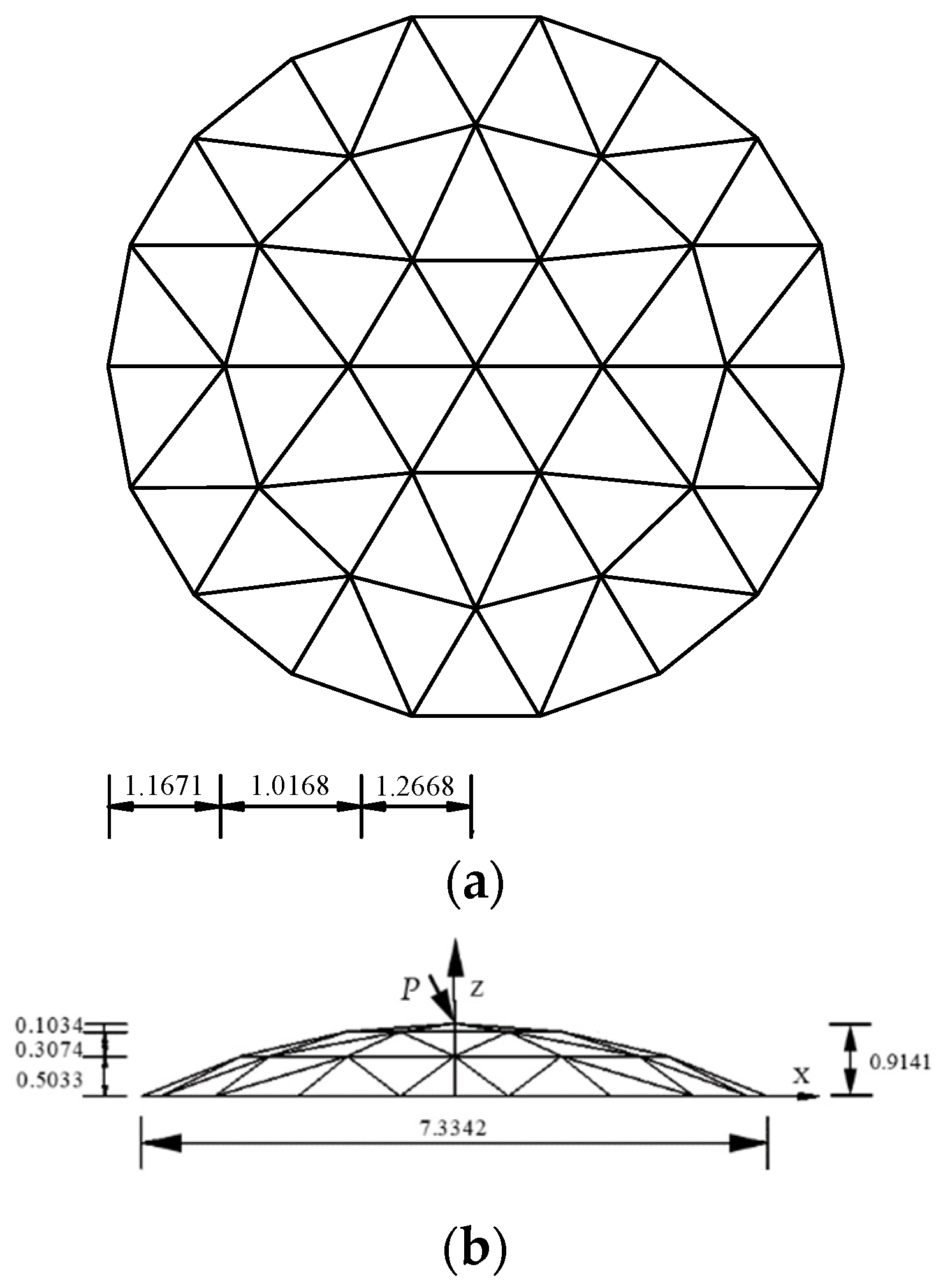
3.1.1. Model Parameters
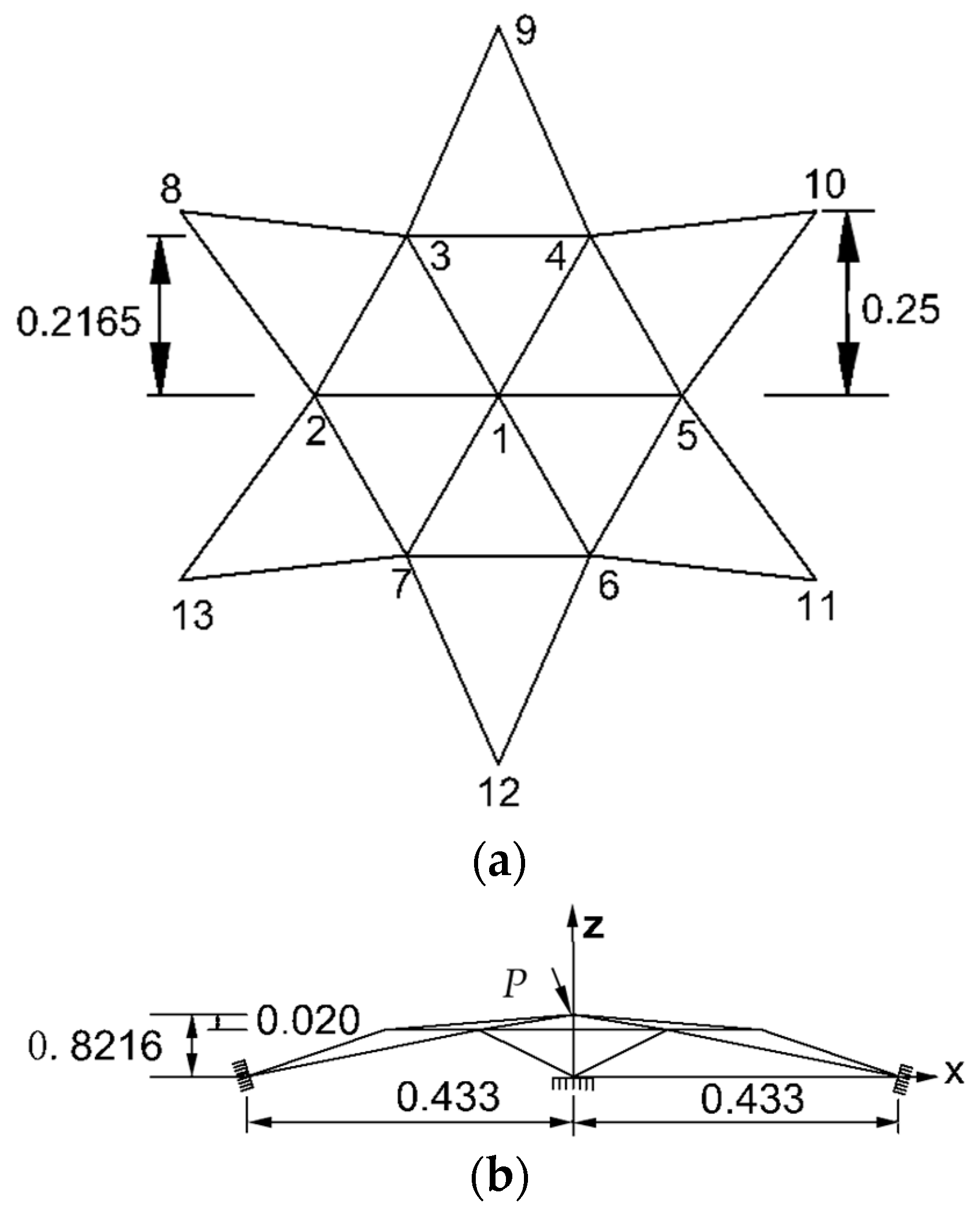
The geometric parameters of the hexagonal flat reticulated shell structure are shown in
Figure 1 [
23]. The material is assumed to be an ideal elastic material (isotropic), the elastic modulus is
E = 3030 MPa, the shear modulus is 1096 MPa, the Poisson’s ratio is 0.3, and the mass density is 7850 kg/m
3. The component adopts a rectangular solid rod with a cross-sectional area of 317 mm
2. The load
P acts downward at vertex 1.
We assume that the components are rigidly connected, and the periphery is 3-dimension fixed hinge support. Furthermore, we model this structure by means of ANSYS software, and the discrete elements of the members are Timoshenko beam elements (beam188).
Figure 1 shows the elements and the corresponding node numbers.
3.1.2. Analysis of Parameters, Calculation of Physical Quantities and Definition of Indicators
The response surface fitting functions considered in this paper mainly include linear polynomials (Lin), complete quadratic polynomials (Quad), and quadratic polynomials with cross terms (Quax). We select the random variable number of each function form as 3, 4, 5, and 6. In this paper, the calculation result of MCS method [
28,
29] is selected as the reference value for optimization and comparison, as it is the critical load closest to the true value. The resulting physical quantities used for comparison include calculation time
t, response surface function accuracy, minimum
and
, etc. Here, we use
e to represent the critical load error between the response surface method and the MCS method, and the sampling times of MC are 10,000.
The accuracy of this method depends not only on its relative error,
e, but also on the accuracy of its critical value function fitting (
). If we select one of the indicators for comparative analysis, the result will be inaccurate. For this reason, we constructed an effective coefficient,
fcec (compound evaluation coefficient), which can comprehensively consider these two indicators and judge the pros and cons of the method, as shown below: In the formula, the closer the
fcec value is to 1, the higher the prediction accuracy of the method.
Note that the software used in the analysis of this paper is ANSYS 19.1, the computer used is a Lenovo brand desktop computer, and the processor is Intel (R) Core (TM) i7-10750H CPU @ 2.60 GHz, with four cores.
3.2. Central Composite Design Allocation Point
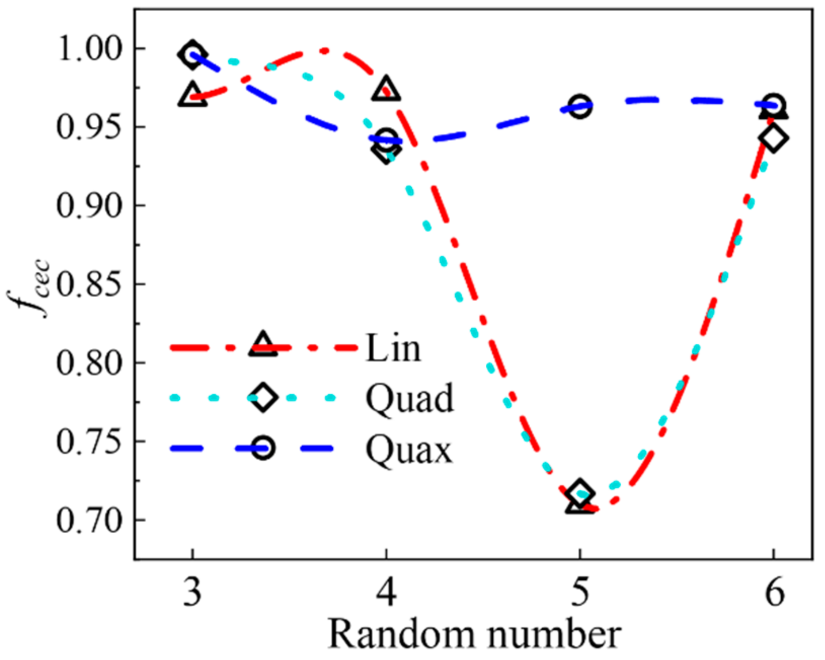
Figure 2 and
Figure 3 show the calculation results using the central composite design (CCD) collocation method in this section.
Figure 2 shows the effective accuracy
fcec of the new method with three fitting functions. In the three cases, they all consider different numbers of random variables. When using the Lin polynomial, the curve of the number of random variables–calculation accuracy is a sine curve of one wavelength, and one of the peaks is very large. When using the Quad polynomial, the fluctuation phenomenon of the curve is similar to the Lin method, and the two curves are very close. When using Quax polynomial, the curve has no significant fluctuations, and the trend is stable. Therefore, given the effective accuracy f and stability, this method’s response surface fitting function is preferably Quax polynomial.
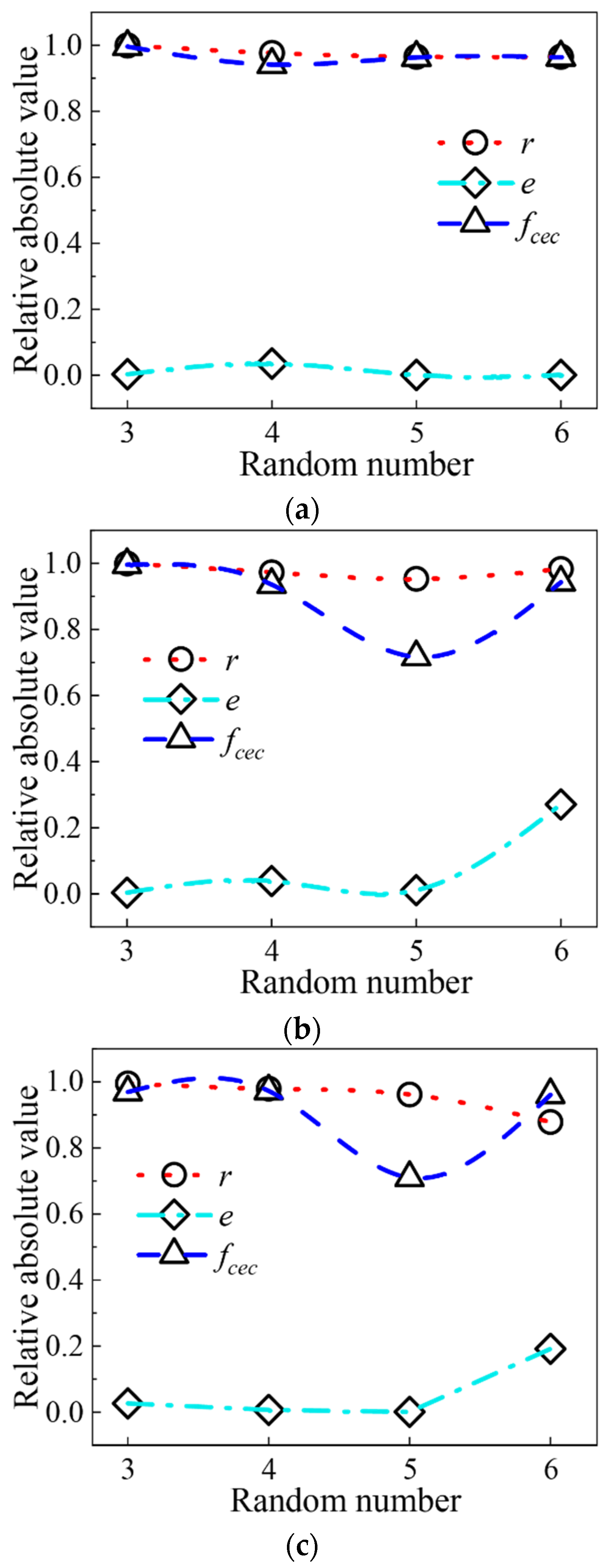
Figure 3a–c further shows the detailed error and precision values of
e,
r and
fcec when the method uses three polynomial fittings.
Figure 3a shows that the
e/
r-random variable curves calculated by this method using Quax polynomials are all stable. At the same time, it shows that the critical load accuracy
e calculated by it is less than 3.70%, which meets the engineering accuracy. At the same time,
Figure 3b,c shows
e,
r, and
f values when adopting the Quad and Lin polynomials in this method, respectively. The stability of their
e/
r//
f-random variable number curve is worse than the result of the Quax polynomial, and the value of
e is larger than the result of the Quax polynomial, 27.09% and 19.18%, respectively, exceeding the usual engineering accuracy of 5%. Therefore, from the various detailed accuracy (error) analyses shown in
Figure 3 above, it can be seen that the Quax polynomial is also the preferred response surface fitting function of this method.
3.3. Box–Behnken Method (BBM) Distribution Point
3.3.1. Comparison of Calculation Accuracy
The above figures prove that the optimal fitting function is the Quax polynomial when employing the central composite design (CCD) collocation method.
Not only CCD method, but Quax polynomial is still the optimal fitting function when using the Box collocation method. This can easily be proven in the same way as in the previous section. Due to space and time constraints, we will not repeat the verification process.
In order to choose a better method from the two collocation methods of Box and CCD, this section adopts the same parameter settings as in
Section 3.2 to calculate and analyze their physical quantities and discriminant indexes, respectively.
Below, we compare the pros and cons of the two distribution points in terms of accuracy and time cost based on the calculation results.
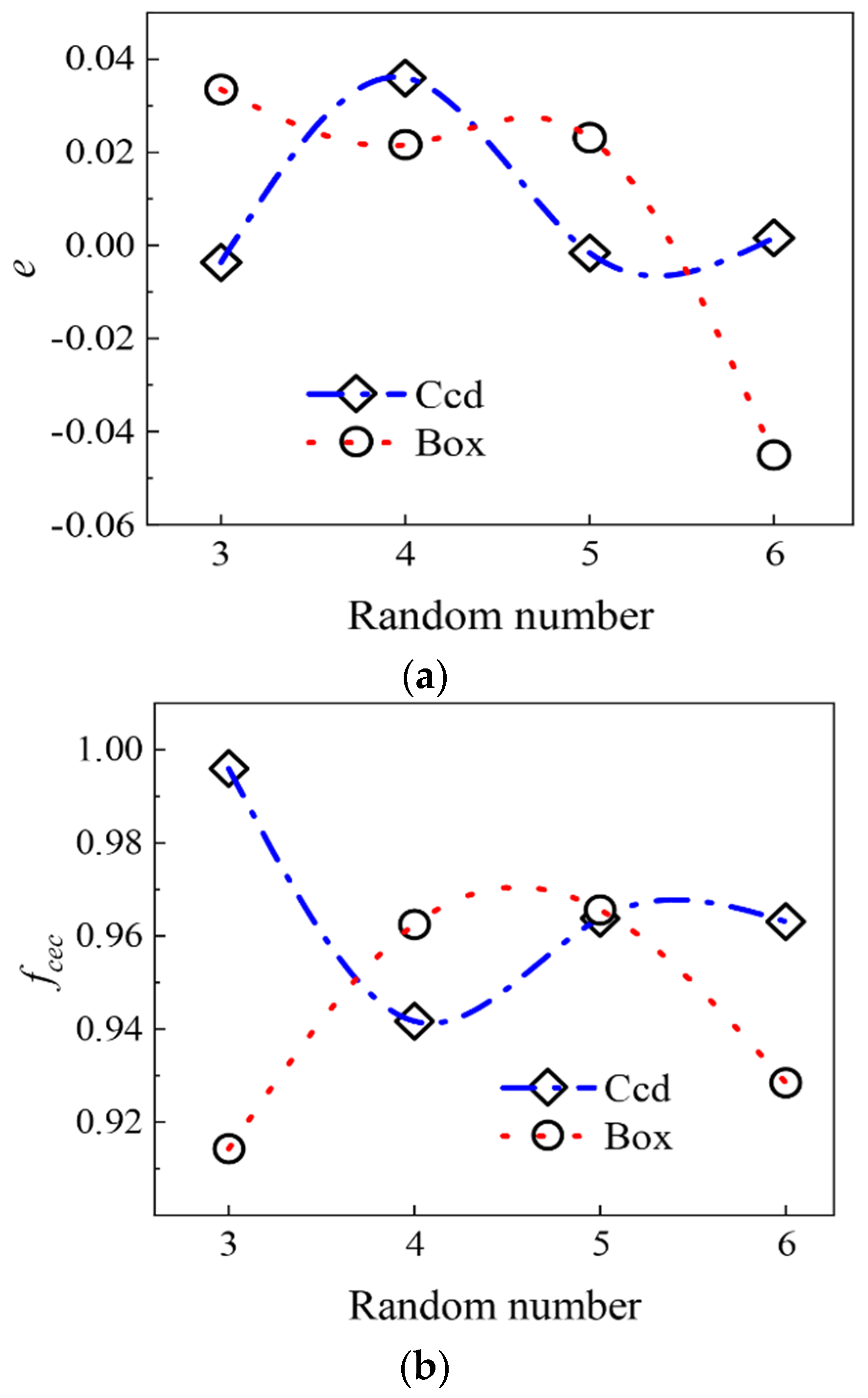
Figure 4 shows the results.
Figure 4b shows that the effective accuracy
range of the CCD collocation method is [0.9417–0.996]. Another method, Box collocation, the accuracy range is [0.9285–0.9656]. The upper and lower limits of the accuracy range when using the CCD collocation method are higher than that of the Box collocation method.
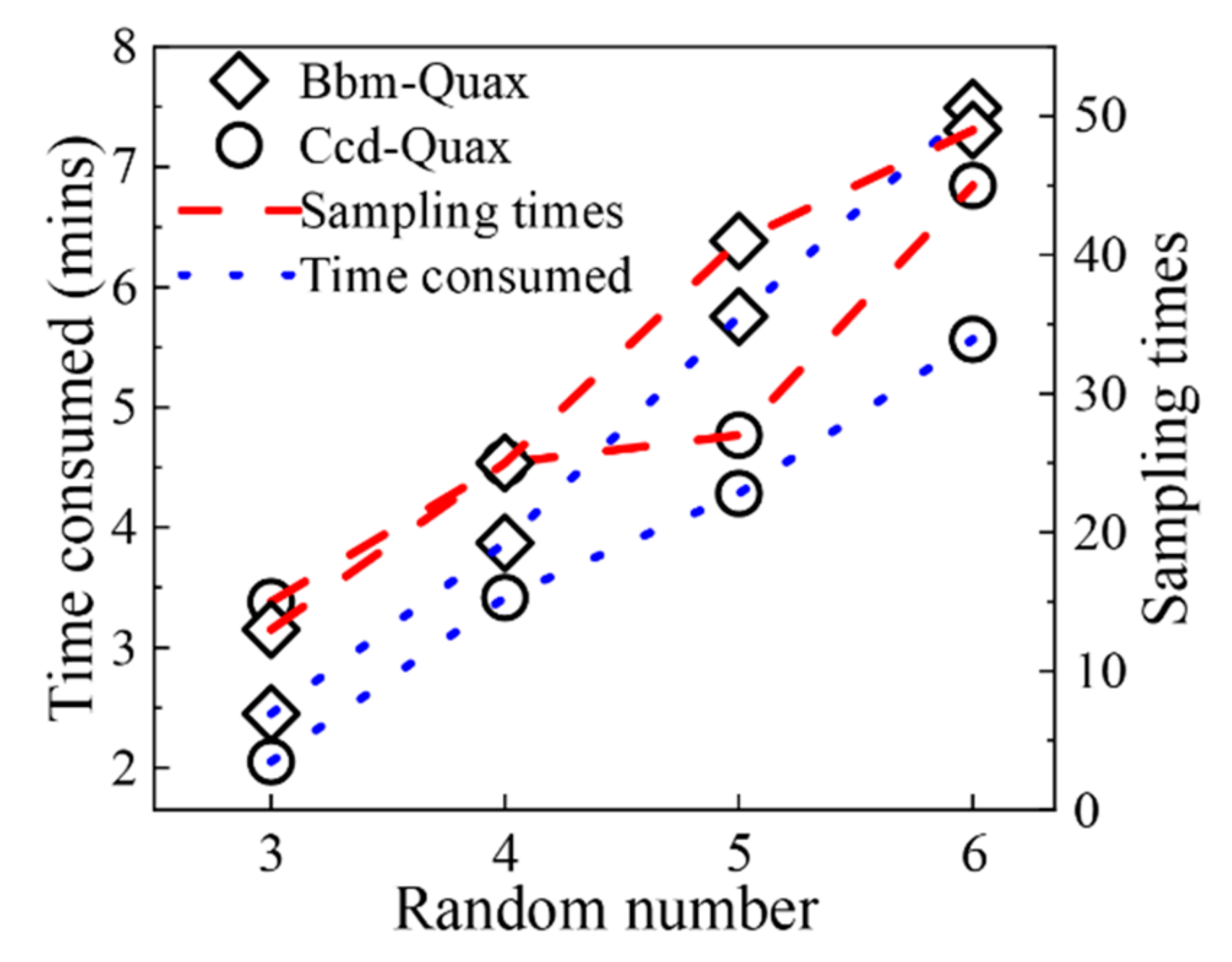
3.3.2. Comparison of Calculation Time and Sampling Times
Figure 5 shows that when the number of random variables is less than 4, the time consumed by the two distribution points differs very little, and the required sampling times differ very little. However, when the number of random variables exceeds 4, the calculation time and sampling times required for CCD collocation points are less than those for box collocation points.
In summary, compared with Box collocation, CCD collocation provides higher accuracy. At the same time, it consumes less sampling times and calculation time (sometimes close). Therefore, CCD is the preferred collocation method for the new method.
4. Effectiveness and Universality of the New Method
We established a new method in the previous section, with its optimized parameters: CCD collocation and Quax polynomials. Further, this section selects the representative traditional reticulated shell structure and the new bionic reticulated shell to verify its effectiveness and universality in the field of space structure.
4.1. Case Analysis of Traditional Reticulated Shell—Taking K6 Reticulated Shell as an Example
4.1.1. Structural Model Parameters
The K6 reticulated shell structure [
17] has a span of 7.3342 m and a vector height of 0.9141 m.
Figure 6 shows the specific geometric dimensions. The rod adopts a hollow round tube, the cross-sectional area of the tube is 55.25 mm
2, the steel density is 7850 kN/m
2, and the material’s elastic modulus is
E = 3030 MPa, the shear modulus is 1.096 × 10
3 MPa, and the Poisson coefficient is 0.3.
The numerical analysis software used in this article is ANSYS. The rods are discrete with Beam188 unit. The periphery of the model is assumed to be supported by a 3D fixed hinge. The load P acts on each node in the direction of gravity.
4.1.2. Analysis of the Parameters
This section compared the optimized new method with the traditional MCS method. The number of random variables selected in four comparisons are 3, 4, 5 and 6, respectively. Every comparison group is sampled 10,000 times. This sample size can reach the initial convergence to determine a minimum number of samples for stability. The comparative analysis is conducted using physical target quantity
,
p* and
, which are defined in Equation (7),
Section 2.2.2 and
Section 3.1.2, respectively.
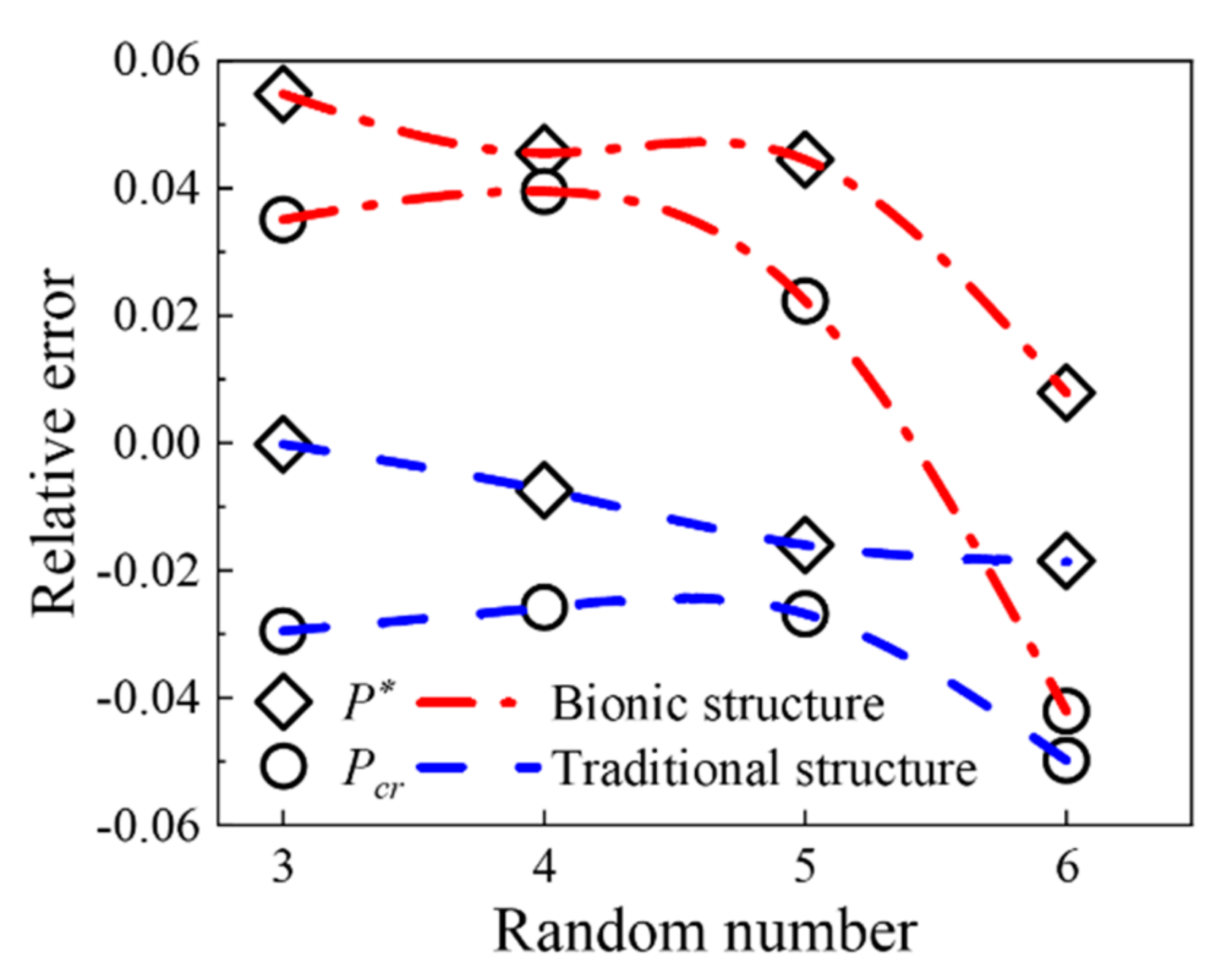
4.1.3. Calculation Results
Figure 7 shows the relative error of the new method and the MCS method when applied to traditional reticulated shells.
We can know from this picture:
- (1)
Compared with the result of MCS method, the relative error of under each random variable number of the new method meets the engineering accuracy requirement, not larger than 5%;
- (2)
The number of different random variables will cause the results of the new method to fluctuate to a certain extent. It shows that when we employ the new method to the traditional reticulated shell, the calculation result has a specific correlation with the random variable number.
4.2. Example Analysis of Bionic Reticulated Shell Structure
After completing the effective verification of the new method when used in traditional reticulated shells, this section further studies its applicability for the new type of bionic reticulated shells, such as applicability for Euryale veins [
39], shells [
40], bamboo vascular bundles [
41] and water spider diving clocks [
42]. The subject of the analysis employs a spiral net shell as an example.
4.2.1. Mathematical and Geometric Models
This example uses the spiral net shell proposed in the literature [
43]. The literature shows that it has a strict shape design [
43], proper meshing, and optimized mechanical properties—somehow, its stable performance is different from the traditional net shell. Its mathematical and geometric models can be found in this document [
43]. However, for the sake of brevity and understanding, its structure and numerical model are shown here.
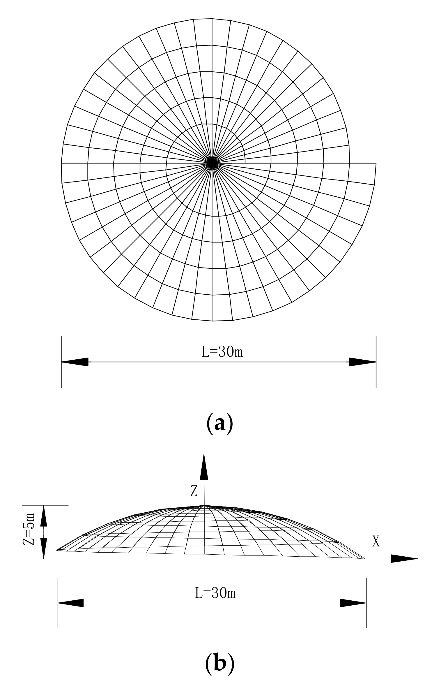
4.2.2. Structural Model
For the new model, a spiral single-layer reticulated shell, structural parameters such as maximum radius (m) and height (m) are 4.8 m and 0.8333 m, respectively, the ring division frequency is 48, and the number of loops is 5. The plan view and elevation view of the corresponding model are shown in
Figure 8.
4.2.3. Finite Element Models
The new reticulated shell uses a hollow round tube. The cross-sectional area of the circular tube is 111.44 mm
2. The mechanical parameters of other materials, analysis software, discrete elements, boundary conditions, and load conditions are the same as those in
Section 4.1.1 and
Section 4.2 calculation parameters.
4.2.4. Calculation Results
Figure 7 shows the relative error of the calculation results of this method and the benchmark method when analyzing the new bionic reticulated shell.
As we can obtain from the figures:
- (1)
The and of this new method under all random variables is not greater than the engineering accuracy (5%), indicating that it is effective.
- (2)
The changing of the number of random defect variables can introduce slight fluctuations into the results of this method. However, from the results of calculation examples in this paper, it does not have a negative effect.
5. Conclusions
This article proposes a new method to meet the dual high requirements of accuracy and efficiency in the stochastic stability analysis of spatial structures, which can significantly improve the engineering application of stochastic stability analysis methods, which were previously limited. In turn, it can greatly improve the application of the original restricted stochastic stability analysis method in engineering.
First, we explained the randomness, fitting and solvability characteristics of this method and its three key algorithms: random, fitting, and critical algorithms.
Then, using a classic structural example and taking the MCS method as the reference method, the new method’s multiple collocation parameters, and fitting functions were optimized. In the optimization, when using the central composite design (CCD) collocation method, the effect is the best when the fitting function employs Quax. Similarly, when using the Box collocation method, the effect of using Quax remains optimal. (Its optimization process is the same as CCD, this article did not discuss it in detail.) Moreover, the CCD method is more accurate than the Box method. It requires less time and less sampling times than (though sometimes close to) the Box method. In summary, CCD collocation method and Quax fitting function are the most suitable for the new method.
Finally, the analysis of calculation examples for traditional reticulated shells and bionic reticulated shells shows that the optimized new method effectively balances efficiency and accuracy. At the same time, it is universal in analyzing spatial structures, including various kinds of reticulated shells. It is foreseeable that the new method is expected to successfully break through the application limitations of the existing stochastic stability analysis method in the actual engineering of space structures.
Author Contributions
Conceptualization, H.L.; Funding acquisition, H.L.; Methodology, H.L.; Resources, X.L. and Z.X.; Writing—review & editing, N.T. and C.C. All authors have read and agreed to the published version of the manuscript.
Funding
This work was supported by the National Natural Science Foundation of China (grant number 51708135, 52068003), the Guangxi Natural Science Foundation (grant number 2019GXNSFAA185057), the Opening Project of Guangxi Laboratory on the Study of Coral Reefs in the South China Sea (grant number GXLSCRSCS201900*), and the Opening Project of Guangxi Key Laboratory of Disaster Prevention and Engineering Safety (grant number 2019ZDK043, 2019ZDK044). Opinions, findings, and conclusions expressed in this paper are those of the authors and not necessarily those of the sponsors.
Institutional Review Board Statement
Not applicable.
Informed Consent Statement
Not applicable.
Data Availability Statement
The raw data required to reproduce these findings cannot be shared at this time due to time limitations. The processed data required to reproduce these findings cannot be shared at this time due to time limitations.
Acknowledgments
The authors are particularly grateful to W.C.X. Ample. He is a freelancer, American citizen of Chinese descent and provided valuable suggestions on the structure and language used of this paper.
Conflicts of Interest
The authors declare no conflict of interest.
Symbol Lists
| Stiffness matrix of structure. |
| Buckling eigenvalue of structure, i = 1, 2, …, m. |
| The ith-order linear buckling mode of the structure. |
| R | Amplitude. |
| Defect pattern vector. |
| Total response mode. |
| Displacement vector of node i in . |
| n | Number of structural nodes. |
| m | Modal participation order. |
| ri | Participation coefficient, independent random variable, i = 1, 2, …, m. |
| Displacement vector of n—node in i—order buckling mode. |
| Function of random variable . |
| Function of random variable . |
| Function of random variable . |
| Response value-stable critical load value. |
| Fitting function of the critical load. |
| Undetermined coefficients of fitting function. |
| Undetermined coefficients of fitting function. |
| Undetermined coefficients of fitting function. |
| Group i random variables, i = 1, 2, …, k. |
| Group i critical load, i = 1, 2, …, k. |
| Number of j random variables of group i data. |
| The critical load value of group i data. |
| Undetermined coefficient. |
| [] | Expansion range of mean point centered expansion. |
| The mean of group i data. |
| μ | The mean of the whole data. |
| f | Factor of model. |
| The standard deviation of group i data. |
| The most unfavorable critical load. |
| Design value of bearing capacity of reticulated shell structure without defects. |
| Structural failure probability under random defects. |
| Z | Reliability function of critical state of structure. |
| E | Elastic modulus. |
| e | Critical load error between response surface method and Monte Carlo sampling method. |
| Accuracy of critical value unction fitting. |
| fcec | Effective coefficient to judge the method by considering e and . |
| Lin | Linear polynomial response surface function. |
| Quad | Complete quadratic polynomial response surface function. |
| Quax | Quadratic polynomial response surface function with cross term. |
| Nodal forces. |
References
- Moon, J.-E.; Kim, B. A Study on Spatial Structures According to Booth Layout at Convention and Trade Exhibition Centers. J. Archit. Inst. Korea Plan. Des. 2013, 29, 71–81. [Google Scholar]
- Orzhekhovskiy, A.; Priadko, I.; Tanasoglo, A.; Fomenko, S. Design of stadium roofs with a given level of reliability. Eng. Struct. 2020, 209, 110245. [Google Scholar] [CrossRef]
- Pál, Á.; Győri, F. Contemporary Changes in the Role and Spatial Structure of Industrial Production in Hungary. Stud. Ind. Geogr. Comm. Pol. Geogr. Soc. 2016, 30, 127–146. [Google Scholar] [CrossRef]
- Ducruet, C.; Notteboom, T. The worldwide maritime network of container shipping: Spatial structure and regional dynamics. Glob. Netw. 2012, 12, 395–423. [Google Scholar] [CrossRef] [Green Version]
- Yan, W.; Wang, T.; Zhang, N.; Liao, S. Study on the wind pressure distribution characteristics and shape optimization of gable roof house with partially protruding plane. J. Disaster Prev. Mitig. Eng. 2020, 40, 395–403. [Google Scholar] [CrossRef]
- Manco, M.R.; Vaz, M.A.; Cyrino, J.C.; Landesmann, A. Thermomechanical performance of offshore topside steel structure exposed to localised fire conditions. Mar. Struct. 2021, 76, 102924. [Google Scholar] [CrossRef]
- Technical Specification for Space Frame Structures: JGJ 7-2010; China Construction Industry Press: Beijing, China, 2010.
- Code for Acceptance of Construction Quality of Steel Structures: GB 50205-2001; China Planning Press: Beijing, China, 2002.
- Ye, X. Stability analysis of steel structure design in construction projects. China Constr. Met. Struct. 2021, 70–71. [Google Scholar] [CrossRef]
- Sharifi, P.; Popov, E.P. Nonlinear Buckling Analysis of Sandwich Arches. J. Eng. Mech. Div. 1971, 97, 1397–1412. [Google Scholar] [CrossRef]
- Batoz, J.-L.; Dhatt, G. Incremental displacement algorithms for nonlinear problems. Int. J. Numer. Methods Eng. 1979, 14, 1262–1267. [Google Scholar] [CrossRef]
- Forde, B.W.; Stiemer, S.F. Improved arc length orthogonality methods for nonlinear finite element analysis. Comput. Struct. 1987, 27, 625–630. [Google Scholar] [CrossRef]
- Bathe, K.-J.; Dvorkin, E.N. On the automatic solution of nonlinear finite element equations. Comput. Struct. 1983, 17, 871–879. [Google Scholar] [CrossRef] [Green Version]
- Pei, Y.; Liu, F.; Ren, S.; Bing, Q. Stable ultimate load analysis of the reticulated shells with curvature of members. J. Shandong Jianzhu Univ. 2021, 36, 96–102. [Google Scholar] [CrossRef]
- Li, H.; Wang, C.; Han, J. Research on Effect of Random Initial Imperfections on Bearing Capacity of Single-Layer Spherical Reticulated Shell. Ind. Constr. 2018, 48, 23–27. [Google Scholar] [CrossRef]
- Zhi, X.; Li, W.; Fan, F.; Shen, S. Influence of initial geometric imperfection on static stability of single-layer reticulated shell structure. Spat. Struct. 2021, 27, 7. [Google Scholar] [CrossRef]
- Zhao, H.; Xu, Y.; Bai, G. Influence of stochastic imperfection field on performance of latticed shell structures. Spat. Struct. 2011, 17, 112–119. [Google Scholar] [CrossRef]
- Rothert, H.; Dickel, T.; Renner, D. Snap-Through Buckling of Reticulated Space Trusses. J. Struct. Div. 1981, 107, 129–143. [Google Scholar] [CrossRef]
- Saafan, S.A. Nonlinear Behavior of Structural Plane Frames. J. Struct. Div. 1963, 89, 557–579. [Google Scholar] [CrossRef]
- Borri, C.; Spinelli, P. Buckling and post-buckling behaviour of single layer reticulated shells affected by random imperfections. Comput. Struct. 1988, 30, 937–943. [Google Scholar] [CrossRef]
- Dong Shilin, Zhan Weidong. Non-linear stability critical loads of single-layer and double-layer and reticulated spherical shallow shells based on continuum analyogy method. Eng. Mech. 2004, 21, 6–14. [Google Scholar] [CrossRef]
- Ikeda, K.; Ohsaki, M. Generalized sensitivity and probabilistic analysis of buckling loads of structures. Int. J. Non-linear Mech. 2007, 42, 733–743. [Google Scholar] [CrossRef]
- Huang, B.; Ren, W. The Koiter’s stability theory and its application. Adv. Mech. 1987, 17, 30–31. [Google Scholar]
- Ohsaki, M.; Ikeda, K. Stability and Optimization of Structures: Generalized Sensitivity Analysis; Springer Science & Business Media: Berlin/Heidelberg, Germany, 2007. [Google Scholar] [CrossRef]
- Ao, H. Applications of the Method of Critical Imperfection Modes to the Analysis of Imperfection Sensitivity of Reticulated Shells; Tongji University: Shanghai, China, 2005. [Google Scholar] [CrossRef]
- Cao, Z.; Fan, F.; Shen, S. Elasto-plastic stability of single-layer reticulated domes. China Civ. Eng. J. 2006, 39, 6–10. [Google Scholar] [CrossRef]
- Li, Y.; Shen, Z. Arch-supported reticulated shell structures and their mechanical behaviors. J. Zhejiang Univ. Eng. Sci. 2001, 35, 645–650. [Google Scholar] [CrossRef]
- Tang, G.; Zhao, H.; Zhao, C. Theoretical and experimental study on the stability of sheet space structures with imperfections. China Civ. Eng. J. 2008, 41, 15–21. [Google Scholar] [CrossRef]
- Fan, T. Ultimate Load of Lattice Shell with Random Imperfection; Wuhan University of Technology: Wuhan, China, 2008. [Google Scholar] [CrossRef]
- Wei, D.; Tu, J. A Probe into Nonlinear Stability of Single-Layer Reticulated Shells by Means of Random Imperfection Modal Method. J. South China Univ. Technol. Nat. Sci. Ed. 2016, 44, 83–89. [Google Scholar] [CrossRef]
- Cai, J.; He, S.; Jiang, Z.; Zhang, Y.; Liu, Q. Investigation on maximum value of initial geometric imperfection in stability analysis of single layer reticulated shells. J. Build. Struct. 2015, 36, 86–92. [Google Scholar] [CrossRef]
- Cai, J.; He, S.; Jiang, Z.; Liu, Q.; Zhang, Y. Investigation on Stability Analysis Method of Single Layer Latticed Shells. Eng. Mech. 2015, 103–110. [Google Scholar] [CrossRef]
- Luo, Y. Research on the Advanced Consistent Mode Imperfection Method for Single-Layer Domes Stability Analysis; Tianjin University: Tianjin, China, 2007. [Google Scholar] [CrossRef]
- Bruno, L.; Sassone, M.; Venuti, F. Effects of the Equivalent Geometric Nodal Imperfections on the stability of single layer grid shells. Eng. Struct. 2016, 112, 184–199. [Google Scholar] [CrossRef] [Green Version]
- Liu, H.; Zhang, W.; Yuan, H. Structural stability analysis of single-layer reticulated shells with stochastic imperfections. Eng. Struct. 2016, 124, 473–479. [Google Scholar] [CrossRef]
- Zhang, Q. Stability of Single-Layer Spherical Reticulated Shell Structures with Random Initial Defects; Hunan University: Changsha, China, 2018. [Google Scholar]
- Onwuamaeze, C.U.; Oladugba, V.A.; Eze, C.M. Optimal prediction variance properties of some central composite designs in the hypercube. Commun. Stat.-Theory Methods 2021, 50, 1911–1924. [Google Scholar] [CrossRef]
- Wang, M.; Zhou, Z.; Wang, Q.; Liu, Y.; Wang, Z.; Zhang, X. Box-behnken design to enhance the corrosion resistance of plasma sprayed Fe-based amorphous coating. Results Phys. 2019, 15, 102708. [Google Scholar] [CrossRef]
- Guan, S. Bionic Research for Dome Greenhouse Structure Based on Euryale (Euryale ferox Salisb.) Leaf Vein; Jilin University: Changchun, China, 2020. [Google Scholar]
- Huang, H. Method for Determining Important Monitoring Members of Space Steel Structure Based on Multiobjective Genetic Algorithm; Harbin Institute of Technology: Harbin, China, 2020. [Google Scholar]
- Palombini, F.L.; Mariath, J.E.D.A.; de Oliveira, B.F. Bionic design of thin-walled structure based on the geometry of the vascular bundles of bamboo. Thin-Walled Struct. 2020, 155, 106936. [Google Scholar] [CrossRef]
- Gu, D.; Yang, J.; Wang, H.; Lin, K.; Yuan, L.; Hu, K.; Wu, L. Laser powder bed fusion of bio-inspired reticulated shell structure: Optimization mechanisms of structure, process, and compressive property. CIRP J. Manuf. Sci. Technol. 2021, 35, 1–12. [Google Scholar] [CrossRef]
- Liu, H.; Li, F.; Yuan, H.; Ai, D.; Xu, C. A Spiral Single-Layer Reticulated Shell Structure: Imperfection and Damage Tolerance Analysis and Stability Capacity Formulation for Conceptual Design. Buildings 2021, 11, 280. [Google Scholar] [CrossRef]
| Publisher’s Note: MDPI stays neutral with regard to jurisdictional claims in published maps and institutional affiliations. |
© 2021 by the authors. Licensee MDPI, Basel, Switzerland. This article is an open access article distributed under the terms and conditions of the Creative Commons Attribution (CC BY) license (https://creativecommons.org/licenses/by/4.0/).


