
A Lightweight Neural Network Based on GAF and ECA for Bearing Fault Diagnosis

College of Mechanical Engineering, Shenyang Ligong University, Nanping Middle Road 6, Shenyang 110159, China
*
Author to whom correspondence should be addressed.
Metals 2023, 13(4), 822; https://doi.org/10.3390/met13040822
Submission received: 12 March 2023
/
Revised: 3 April 2023
/
Accepted: 17 April 2023
/
Published: 21 April 2023
(This article belongs to the Special Issue Quality Prediction and Control Technology Design for Intelligent Manufacturing)
Abstract
:A lightweight neural network fault diagnosis method based on Gramian angular field (GAF) feature map construction and efficient channel attention (ECA) optimization is presented herein to address the problem of the complex structure of traditional neural networks in bearing fault diagnosis. Firstly, a GAF is used to encode vibration signals into a temporal image. Secondly, the double-layer separation residual convolution neural network (DRCNN) is used to learn advanced features of the sample. The multi-branch structure is used as the receiving domain. ECA learns the correlation between feature channels. The extracted feature channels are adaptively weighted by adding a small additional computational cost. Finally, the method is tested and evaluated using wind turbine bearing data. The experimental results show that, compared with the traditional neural network, the DRCNN model based on GAF achieves higher diagnostic accuracy with less parameter calculation.
1. Introduction
With the development of industry, energy development has become crucial to driving social development. Energy is being extracted in large quantities and used in a crude manner. This has led to a gradual depletion of non-renewable energy sources. At the same time, the excessive use of fossil energy is causing increasing environmental pollution. This poses a serious threat to the sustainable development of the human economy and society. Countries around the world are actively developing policies on new energy sources in order to change the energy landscape in their countries. Wind energy is an important clean technology. Among the renewable energy technologies, wind power generation is a relatively mature and commercially promising option. The development of wind power is of great importance in improving the energy structure, protecting the ecological environment, ensuring energy security, and achieving sustainable economic development. It has become a worldwide consensus to vigorously develop wind power generation [1,2].
The wind turbine works in an alternating load environment. It is prone to failure. Most of the units are located in remote suburban areas, so manual inspections are costly, and routine maintenance is a major challenge. Rolling bearings are an important component of wind turbines. The health of rolling bearings is the basis for the stable operation of wind turbines. It is important to carry out research on the fault diagnosis of wind turbine bearings [2,3,4].
Among the bearing fault diagnosis methods, there are two main categories: data-driven methods, and signal analysis methods [5,6,7]. In terms of signal analysis methods, some recent research advances have been made. Wang Xiaolong et al. presented a diagnosis method based on the improved empirical wavelet transform (IEWT) [8]. The constructed wavelet is used to separate the sensitive modal components from the angular domain signal. The transient energy amplification feature of the sensitive modal component is calculated by means of a frequency-weighted energy operator. The engineering field signal proves the effectiveness of this method. Wang Huaqing et al. presented a method to obtain comprehensive fault parameters using the least squares mapping (LSM) technique [9]. This method can improve the diagnostic sensitivity of symptom parameters. Examples of bearing diagnostics verify that the method is effective in extracting fault characteristics such as outer raceways, inner raceways, and roller elements of bearings. This method can be used for fault diagnosis under the condition of variable speed. An EWT-MDS method was presented by Tan Yuan et al., it combines empirical wavelet decomposition and multidimensional scale transformation [10]. In this method, the bearing signal is decomposed by a self-adaptive empirical wavelet. The change characteristics of each mode are analyzed by information entropy. By combining multidimensional scale transformation algorithms, the synergistic variation pattern of each component in high-dimensional space is obtained, thereby enabling bearing fault diagnosis. These methods rely on the engineering experience of technicians. It is difficult to make the related technologies universal. Especially under variable working conditions, the vibration signal has the characteristics of modulation, pulse impact interval, unstable sampling phase, and low signal-to-noise ratio. Fault diagnosis methods based on signal analysis are limited. Data-driven methods can significantly remove such limitations. Data-driven methods are based on the use of features inherent in the data for fault diagnosis studies. These methods can effectively and quickly process signals. Accurate detection results are provided. The serendipity of manually extracted features is avoided. Therefore, data-driven methods have recently been widely studied in the field of mechanical fault diagnosis.
Most data-driven methods are based on machine learning. As an important branch of machine learning, deep learning (DL) has recently been widely used in fault diagnosis. DL is an effective technique in data-driven methods, and it is different from one-dimensional vibration signal information. Such methods use the intrinsic characteristics of sample data for fault detection studies. Convolutional neural networks (CNNs) in DL are particularly suitable for processing two-dimensional images, due to their tight connections between levels in the spatial structure. They adaptively extract rich correlation properties between pixel points from the image. The layout of the CNN model is closer to an actual biological neural network than to an artificial neural network. Weight sharing reduces the complexity of the network. In the field of image processing, images can be used directly as inputs to a convolutional neural network model. The pattern recognition process of feature classification is avoided. Convolutional neural networks are more widely used than traditional neural networks. They are also playing a huge role in the rise of deep learning.
In terms of DL signal analysis methods, some recent research advances have been made. Chen et al. used continuous wavelet transform (CWT) to process the bearing vibration data into a wavelet time-frequency graph [11]. Then, a square pool structure CNN was constructed to extract advanced features. The extreme learning machine was used as a strong classifier. The validity of the method was verified using a dataset of motor bearings. Pham et al. transformed the raw data into spectrograms using STFT. The spectrograms were sent to the neural network for fault classification [12]. A high level of accuracy was achieved. Wang Nini et al. presented a rolling bearing fault diagnosis model based on multiscale deep convolution network feature fusion. A multiscale feature fusion module was built into the network structure to extract features at different levels of the fault sample. Precise classification of different faults was achieved [13]. Wang et al. presented an image coding method based on a Gramian angular field (GAF). The validity of this method was verified by a tiled CNN. The GAF can maintain the time dependence of the signal vibration sequence and alter the original data distribution to make it easier to distinguish from Gaussian noise [14].
CNNs have been used in mechanical fault diagnosis by a large number of researchers. In order to obtain better diagnostic accuracy, the designed neural network is often too deep and too wide, which brings about complex calculations and high memory consumption. Thus, the economic cost of data storage is increased. Applications in embedded mobile devices are limited. Therefore, on the basis of ResNet, inverted residual structure, and depth separable convolution, this paper presents the design of a double-layer separated residual convolution module as the main structure [15,16,17]. The multi-branch structure is used as the initial information-receiving domain of the sample. In order to enhance the nonlinear expression ability of the model, efficient channel attention (ECA) is introduced into the structure to capture the local features in information transmission [18]. A double-layer separation residual CNN (DRCNN) model with small storage, low latency, and high accuracy is constructed. Firstly, a GAF is used to encode the one-dimensional vibration signal. The generated timing diagram can maintain the temporal correlation of the signal in the image data without losing the characteristics of the original signal. Then, the ECA module is used to optimize the model, so that the model can adaptively allocate computing resources. Details of the features associated with the type of fault can be captured, and the learning ability of the model is improved. Finally, by comparison with other models, the test proves that the DRCNN not only has a stable structure but also has a low calculation cost, which can meet the potential demand of actual diagnosis.
2. Theoretical Background
2.1. Gramian Angular Field
A GAF can convert one-dimensional time series in a Cartesian coordinate system into a polar coordinate system. It is able to retain the complete information of the signal. It also preserves the dependence of the signal on time. Trigonometric functions are used to generate the GAF matrix map, and 2D images are obtained. After the signal data are converted to image data, the advantages of CNNs in image classification and recognition can be fully used for modelling. The specific process is as follows:
(1) Suppose the given time series is , where xi is the i-th sample signal, i = 1,2,…,n, and n is the number of sampling points. In order to ensure that the inner product value is not biased towards the maximum value in the sequence, the series is mean-normalized by Equation (1). Sequence values are scaled to [−1,1].
(2) xi represents the value at the i-th moment of the original signal sequence. is the normalized vibration sequence. Polar coordinates are used to represent the normalized time series. It can be expressed as follows:
where is the cosine of the encoded angle, ti is the timestamp, r is the radius and maintains time dependence, and N is the constant factor of the regularized system. The whole encoding is bijective, and losing information is almost impossible.
(3) The Gram matrix shows the relationships between features, as well as the relationships between features and dimensions. After the inner product, multiscale representation information is obtained. The main diagonal element reflects information about the feature itself. Other elements reflect the closeness of different features. The GAF after converting the signal sequence to the polar coordinate system is defined as follows:
where I is the unit row vector and is the transpose of .
2.2. Depthwise Separable Convolution
Depthwise separable convolution is quite different from normal convolution. It is a form of decomposed convolution. Replacing standard convolution with depthwise separable convolution reduces the computational and parametric volume of the model during convolution. In this way, the computational speed of the model can be increased. This enables the network model to be lighter. This is the core structure that enables CNNs to achieve lightweight feature extraction.
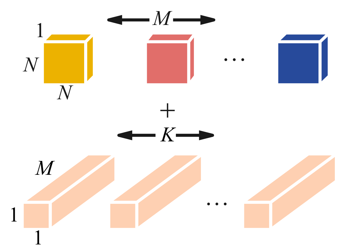
The standard convolution is shown in Figure 1. The standard convolution kernel size is N × N. The number of channels is M. The number of convolution kernels is K. The size of the input feature map is H × W × C. The computational cost of standard convolution is N × N × K × M × H × W.
Depthwise separable convolutions are designed to replace standard convolutions. They can reduce the amounts of calculations and parameters of the model during the convolution process. The network model can be lightweight. Depthwise separable convolution consists of depthwise convolution and pointwise convolution, as shown in Figure 2. Each kernel function of depthwise convolution is applied to a single input channel. The feature maps generated by DW are weighted and combined in the depth direction with PW. In this way, the input and output have the same size. The computational cost of depthwise separable convolution is N × N × M × H × W + M × K × H × W.
The ratio of depthwise separable convolution and standard convolution can be expressed as follows:
where K is greater than 1. The computational cost of depthwise separable convolution is approximately equal to of the standard convolution.
2.3. Efficient Channel Attention
The specific use of channel attention in CNNs is as a separate feature processing module. This module acquires the weights of each channel of the input feature map. It learns the corresponding features for each channel autonomously. Based on the value of the weights, the CNN is able to determine which features are important and which features are redundant in the current task. A greater weight is given to the important features. A very small weight is given to the redundant features. ECA is a representative model of channel attention mechanism.
The given non-dimensionality-reduction aggregated feature is . Channel attention can be determined as follows:
where W is a C × C parameter matrix.
In order to obtain the details of local information and ensure the efficiency and effectiveness of the model, the band matrix Wk is defined as follows:
where Wk has K × C parameters. All channels share the same learning parameters. is determined as follows:
where yi is the set of k adjacent channels of . The weight of yi is calculated by considering the correlation of k adjacent messages in its vicinity. This method implements information interactions through one-dimensional convolution. The size of the convolution kernel is k. The ECA module is obtained as follows:
where C1D is a one-dimensional convolution. There is a mapping relationship between k and C. The channel dimension C can be expressed as follows:
The linear mapping relationship is the simplest. However, it is too limited. The channel dimension C usually is set to a power of 2. A nonlinear mapping relationship can be obtained as follows:
By taking the logarithm of C, k can be obtained as follows:
where odd represents the nearest odd number. Based on the requirement for a ratio between the number of channels C and the size of the convolution kernel, b is set to 1 and is set to 2. The input features are processed by global average pooling. The correlation between channels is obtained by each channel and its k-nearest neighbors. Then, 1D convolution is performed. Finally, the channel attention is learned through the sigmoid activation function. The ECA module is shown in Figure 3.
3. Model Structure Design
3.1. Feature Extraction Layer
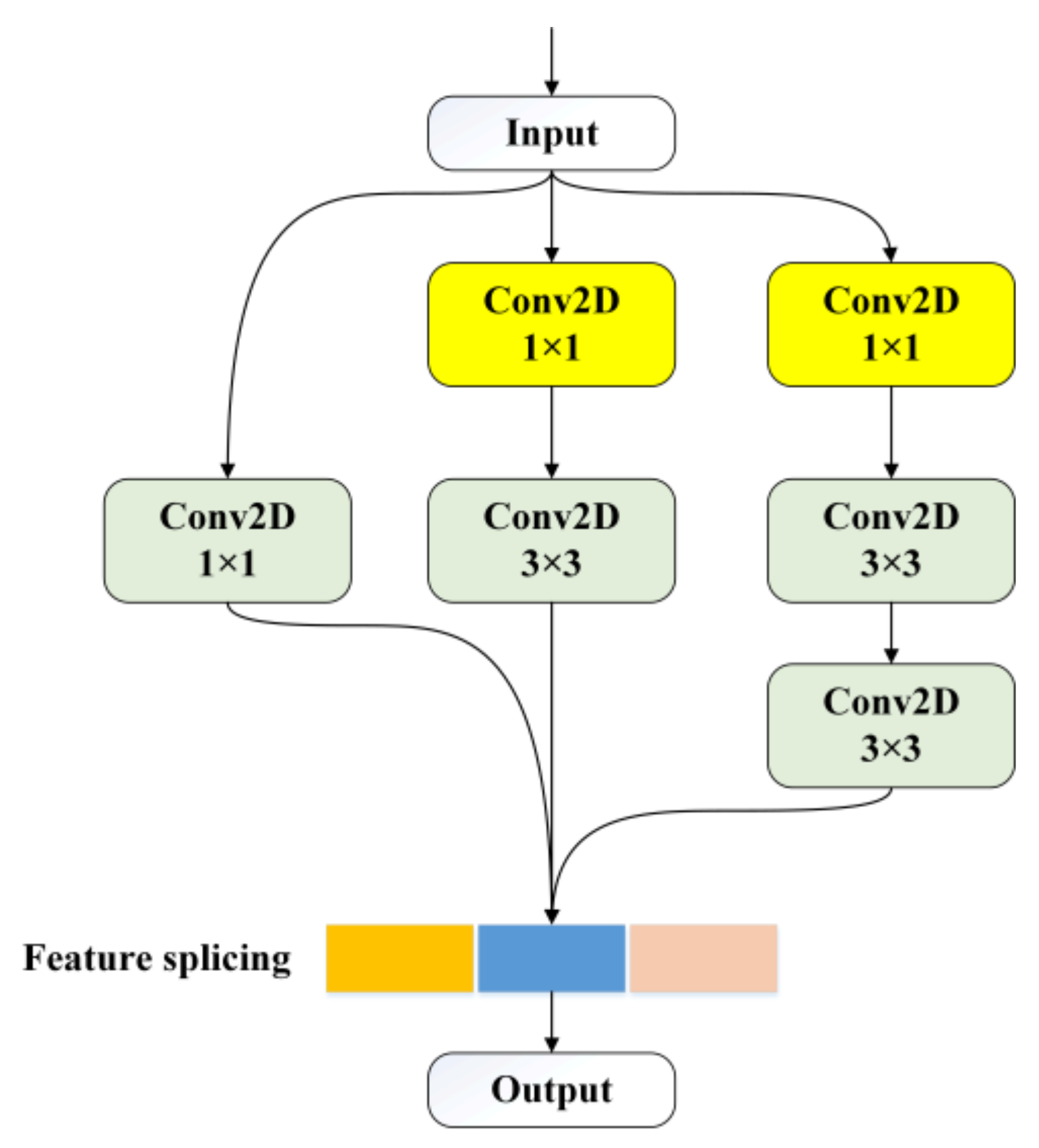
The DRCNN is divided into a feature extraction layer and a linear classification layer. In the feature extraction layer, a double-layer separation residual convolution (DRC) is designed. This module acts as the main body of the structure. The DRC includes three 1 × 1 convolutions, two DW modules, three BN layers, one shortcut branch, and one ECA-Net, as shown in Figure 4.
The detailed steps are as follows:
The input features are mapped to a high-dimensional space by 1 × 1 convolution. This can increase the number of channels.
A DW convolution with kernel size 3 × 3 and stride 2 is used for downsampling feature extraction.
The correlation between acquired features is analyzed by the ECA-Net attention mechanism. Weights are adaptively weighted, computational resources are reallocated, and the nonlinear expressivity of the model is increased.
The ECA-optimized features are again convolved with a DW of stride 1. The convolved features of size 1 × 1 and the shortcut branch are added. In this way, a sparse representation of the sample features can be obtained. It can also effectively slow down the gradient diffusion degradation and explosion in gradient propagation in deeper network structures.
Batch normalization (BN) is added to each layer of convolution. BN can reduce the distribution of the input value of any neuron in the neural network layer to a standard normal distribution through the whitening operation. A standard normal distribution has a mean of 0 and a variance of 1. The fixed distribution form avoids the shifting of covariates within the network. The derivative corresponding to the activated input value is far away from the derivative saturation region. At this time, a small input change will produce a large change in the loss function [19], and neural network convergence can be accelerated. The initial feature of the sample adopts a multiscale branching structure (MSBS). The purpose is to obtain the multilayer receptive field information of the sample. The MSBS is only used once in the sample’s initial input stage. The specific structure of the MSBS is shown in Figure 5.
3.2. Linear Classification Layer
The linear classification layer uses a nonlinear activation function h-swish (HS) instead of the rectified linear unit (ReLU). Many software and hardware frameworks provide optimized implementations of ReLU. In quantized mode, HS has lower model accuracy loss than other sigmoid-shaped approximation functions. HS is a segmentation function. It can reduce the number of memory accesses and greatly reduce the cost of latency [20]. It is expressed by Equation (12) and Figure 6.
3.3. Parameter Introduction
The detailed parameters of the fault diagnosis module DRCNN are shown in Table 1. In Table 1, t is the expansion factor of the first 1 × 1 convolution in the DRC module. It can control the dimensions of feature enhancement. In Table 1, s is the step size of the move. GAP is used to replace a fully connected layer to reduce the amount of computation.
4. Test Verification
4.1. Data Preprocessing
The performance of the DRCNN model was verified by the collected data. The dataset used was derived from the vibration data of the generator bearing of a wind farm in Tianjin, China. The generator model was DASAA-5023. The sampling frequency was 16,384 Hz, and the rotation speed was 1780 r/min. It was divided into four different bearing states: rolling element failure, inner-ring failure, outer-ring failure, and normal state. In order to ensure that each sample contained at least one cycle, the number of intercepted data points was determined as follows:
where fs is the sampling frequency, fv is the rotation speed, and fp is the number of intercepted data points.
In order to reduce the overfitting of the model and enrich the samples of the dataset, the sample set was enhanced and expanded by means of sliding window sampling. The calculation formula was as follows:
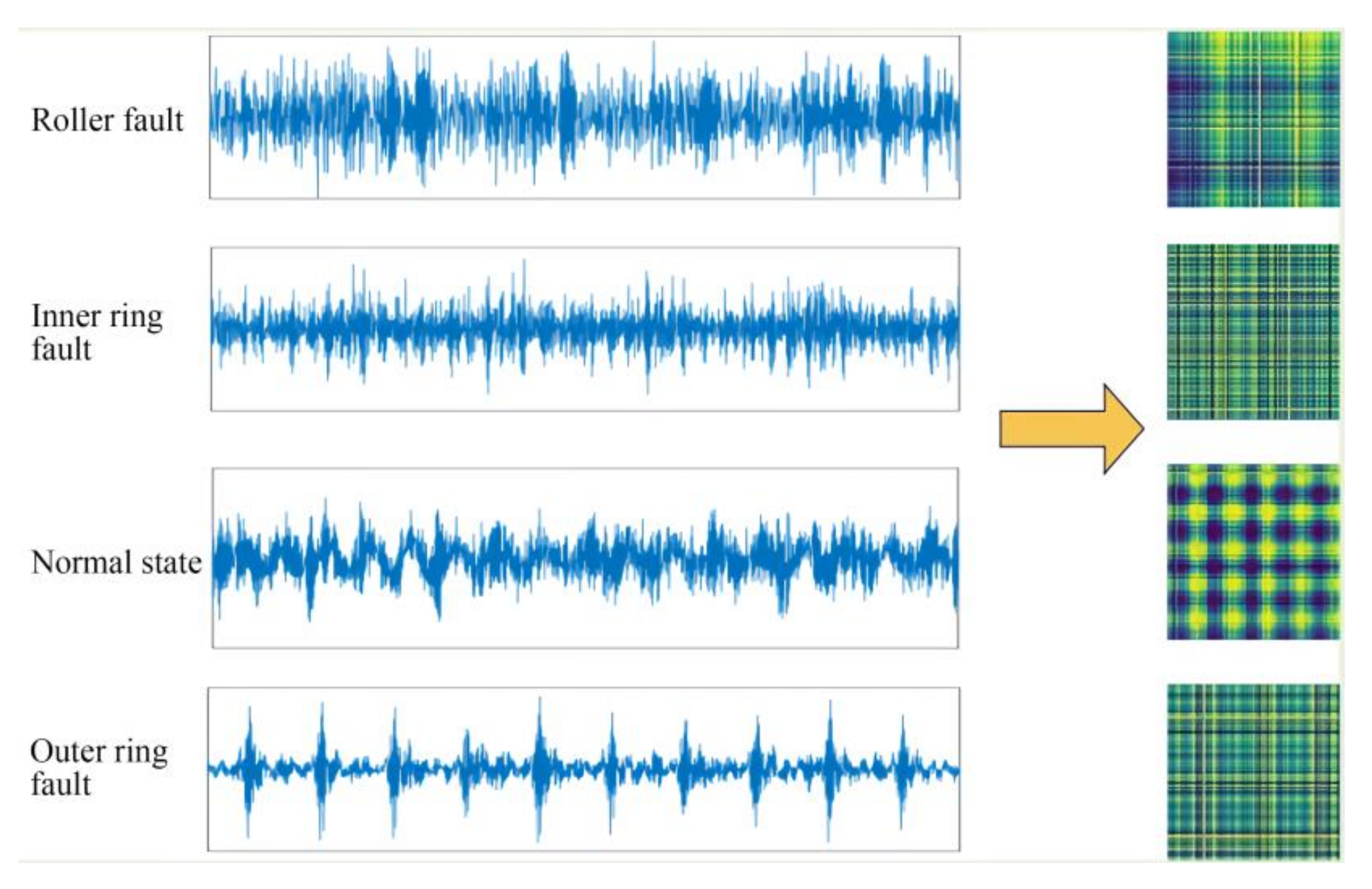
where N is the number of samples, L is the length of the signal data, s is the step size of the sliding window, and floor means round down. Each segment of the truncated data was GAF-converted; s was attached with 300, while fp was attached with 560. A three-channel GAF map with a pixel size of 128 × 128 was obtained. Figure 7 shows the GAF diagrams corresponding to the time-domain waveforms in the four states. The number of each sample type was 1090. The total sample size was 4360. In total, 70% of the samples were used as the training set, 20% of the samples were used as the validation set, and 10% of the samples were used as the test set.
4.2. Experimental Method
The optimizer chooses adaptive moment estimation (Adam). Adam can dynamically adjust the learning rate of the training parameters, and it can smooth the parameters. The initial learning rate was set to 0.001. The number of training sessions was 200. In order to make the weights converge faster and avoid falling into the locally optimal point, a small-batch training method was adopted. The small batch was set to 64. The training loss function is a cross-entropy function, and the formula is as follows:
where m is the number of samples, y is the real sample category, is the predicted sample category, and n is the sample category.
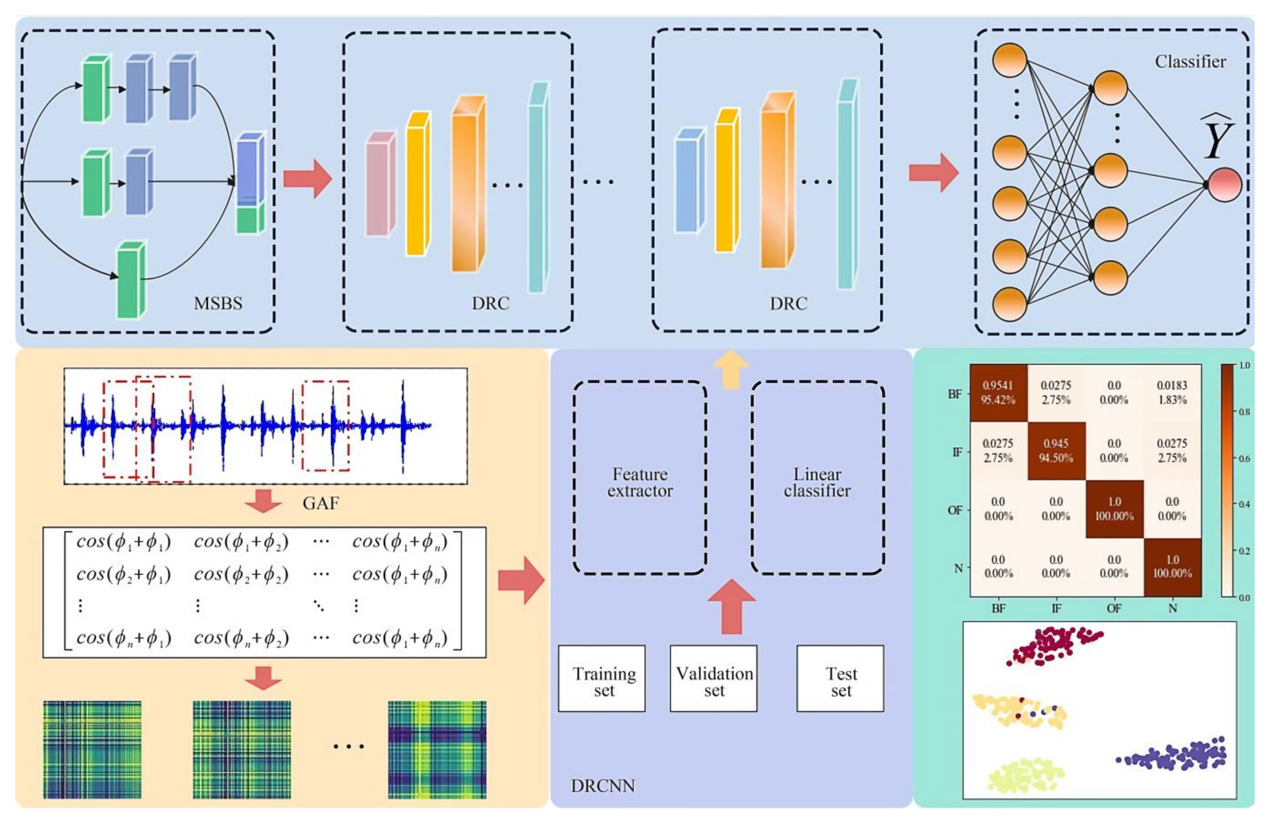
The diagnosis process is shown in Figure 8.
4.3. Results and Evaluation
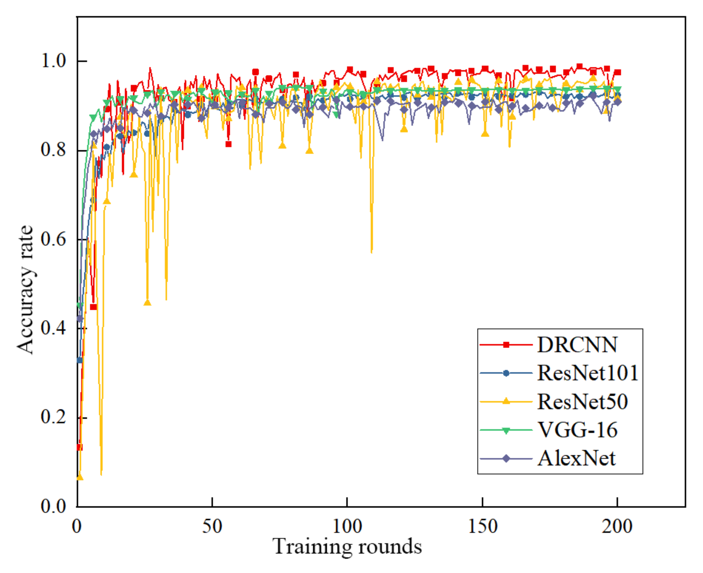
The GAF sample set was used as the input. The performance results of the DRCNN, AlexNet, VGG-16, ResNet50, and ResNet101 models in 200 training sessions are shown in Figure 9 and Figure 10. The results show that the top-1 accuracy rate of the test set was above 90%. When the number of iterations was around 10, the loss value gradually converged, and the model remained stable. There was no overfitting, due to the excellent feature description capability and learnability of the GAF mapping in signal classification. In particular, the DRCNN was faster than the other models, with an accuracy of 97.35%, due to the adequate feature extraction capability of the deep structure layer of the DRCNN. ResNet50 showed a certain oscillation in the test set. Vgg-16 did not converge when the accuracy rate reached around 94.2%. AlexNet had a lower accuracy of 91.17%.
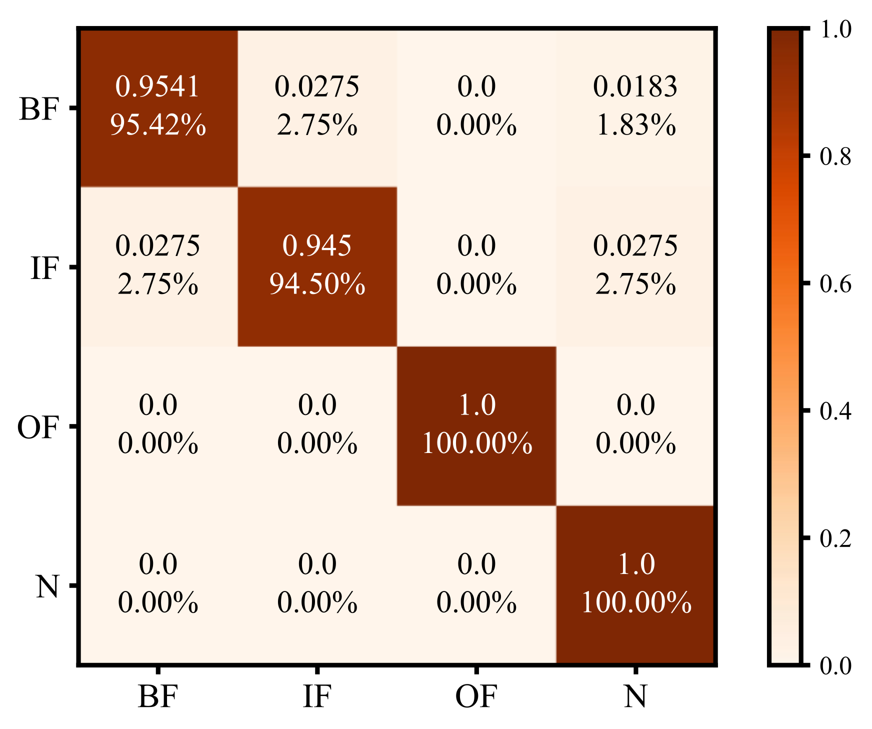
Figure 11 shows the classification of the DRCNN on the confusion matrix diagram. In the figure, the ordinate is the real category, the abscissa is the prediction category, and the diagonal line indicates the correct prediction accuracy of four types of samples. It can be observed from the figure that the DRCNN made a very accurate prediction for the normal sample and the outer-ring sample, while there were some errors in the discrimination of the rolling element and the inner ring, among which about 2% of the fault samples were predicted to be normal samples. This is consistent with the actual observation, because the sensor was close to the outer ring, and the amplitude of the collected signal was often larger than that of the inner ring, so the fault of the outer ring was relatively easy to find. The characteristic frequency of the fault of the rolling element was too small and was often submerged in noise.
Table 2 presents the accuracy, number of parameters, reasoning time, floating point operations per second (FLOPs), and accuracy fluctuation of different models. In deep learning, FLOPs is a performance unit that measures the complexity of the model and evaluates the computing power consumed by the model to complete a forward propagation. The models with lower FLOPs can be better applied in practice. It can be seen from the table that, compared with other models, when the input sample size was 128 × 128, the FLOPs of the DRCNN was 0.14 G, making it far less complex than the other models. The FLOPs of the DRCNN were one-fortieth of those of VGG-16. Among them, the reasoning time of the DRCNN was the shortest, at 7 s. The parameter quantity of the DRCNN was also the smallest, at 5.281 MB. The number of VGG-16 parameters was 25 times higher than that of the DRCNN. The accuracy of the DRCNN was 97.35%. The DRCNN was also the most stable in terms of accuracy fluctuations. It had a fluctuating accuracy range of ±0.1%. The above results show that the DRCNN is lightweight while ensuring accuracy.
5. Conclusions
Aiming at the fault identification of rolling bearings of wind turbines, a lightweight neural network diagnosis method is presented herein. Through the experimental verification of bearing data, the following conclusions could be drawn:
(1) In this paper, the GAF method was used for the two-dimensional transformation of one-dimensional vibration signals. Good accuracies were obtained in the training of different models. This shows that GAFs have excellent detail characterization capability and CNN-learnable capabilities for the vibration data of bearings.
(2) The lightweight neural network diagnosis model DRCNN constructed in this paper takes the double-layer separation residual convolution module as the network’s main body to replace the standard convolution module, and its amounts of parameters and calculations are significantly reduced. The nonlinear activation function HS is used instead of the rectified linear unit. The number of memory accesses is reduced, and the latency costs are significantly reduced.
(3) Compared with Vgg-16, ResNet50, ResNet101, and AlexNet, the comprehensive performance of the DRCNN was better. The number of parameters for the DRCNN was reduced by 129.021 MB compared to VGG-16. The duration of the DRCNN was reduced by 18 s compared to VGG-16. The FLOPs were reduced by 5 G compared with VGG-16. These advantages offer possibilities for the embedded system deployment of fault diagnosis models. These can also contribute to the development of renewable energy sources.
Furthermore, wind turbine bearings are characterized by a large number of types and models. Carrying out a generic model design for all bearings would be a very meaningful direction for research. The CNN fault diagnosis method has many hyperparameters, most of which are set based on experimental experience. The steps are complex, and the stochastic influence is complicated. These hyperparameters have a certain impact on the training accuracy and inference time of the model. Subsequent work can be carried out on excellent intelligent search and adjustment methods to determine the optimal parameters for machine learning. This will help to reduce the time spent on setting parameters. It will also allow the model to achieve better diagnostic performance.
Author Contributions
Conceptualization, X.G. and Y.X.; methodology, X.G. and T.L.; software, X.G. and Y.X.; validation, X.G. and Y.T.; formal analysis, Y.T.; investigation, Y.T.; resources, Y.T.; data curation, Y.X. and T.L.; writing—original draft preparation, X.G.; writing—review and editing, Y.X. All authors have read and agreed to the published version of the manuscript.
Funding
This work was supported by the Scientific Research Fund of the Department of Education of Liaoning Province, China (LJKZZ20220037).
Data Availability Statement
The data presented in this study are available upon request from the corresponding author. The raw/processed data needed to reproduce these findings cannot be shared publicly at this time, as they are also part of an ongoing study.
Conflicts of Interest
The authors declare no conflict of interest.
References
- Bildirici, M.; Ersin, O. An Investigation of the Relationship between the Biomass Energy Consumption, Economic Growth and Oil Prices. In Proceedings of the 4th International Conference on Leadership, Technology, Innovation and Business Management (ICLTIBM-2014), Istanbul, Turkey, 19–21 November 2014. [Google Scholar]
- Bildirici, M.; Ersin, O. Nexus between Industry 4.0 and environmental sustainability: A Fourier panel bootstrap cointegration and causality analysis. J. Clean. Prod. 2023, 386, 135786. [Google Scholar] [CrossRef]
- Xiao, Q.J.; Luo, Z.H. Early fault diagnosis of the rolling bearing based on the weak signal detection technology. In Proceedings of the 2016 14th International Conference on Control, Automation, Robotics and Vision (ICARCV), Phuket, Thailand, 13–15 November 2016. [Google Scholar]
- Chen, X.F.; Guo, Y.J.; Xu, C.B.; Shang, H.B. Summary of research on fault diagnosis and health monitoring of wind power equipment. China Mech. Eng. 2020, 31, 175–189. [Google Scholar]
- Gao, Z.; Cecati, C.; Ding, S.X. A survey of fault diagnosis and fault-tolerant techniques-Part I: Fault diagnosis with model-based and signal-based approaches. IEEE Trans. Ind. Electron. 2015, 62, 3757–3767. [Google Scholar] [CrossRef]
- Chen, H.M.; Meng, W.; Li, Y.J.; Xiong, Q. An anti-noise fault diagnosis approach for rolling bearings based on multiscale CNN-LSTM and a deep residual learning model. Meas. Sci. Technol. 2023, 34, 0450130. [Google Scholar] [CrossRef]
- Jiang, Z.H.; Zhang, K.; Xiang, L.; Yu, G.; Xu, Y.G. A time-frequency spectral amplitude modulation method and its applications in rolling bearing fault diagnosis. Mech. Syst. Signal Process. 2023, 185, 109832. [Google Scholar] [CrossRef]
- Wang, X.L.; Yan, X.L.; He, Y.L. Fault diagnosis of wind turbine bearing based on IEWT energy order spectrum under variable speed. Acta Energ. Sol. Sin. 2021, 42, 479–486. [Google Scholar]
- Wang, H.Q.; Sun, L.K.; Chen, H.P. Feature extraction method based on pseudo-Wigner-Ville distribution for rotational machinery in variable operating conditions. Chin. J. Mech. Eng. 2011, 24, 661–668. [Google Scholar] [CrossRef]
- Tan, Y.; Sun, W.L.; Wen, G.R.; Huang, X. Wind turbine bearing deterioration trend identification and fault diagnosis based on EWT-MDS. Acta Energ. Sol. Sin. 2018, 39, 3511–3518. [Google Scholar]
- Chen, Z.; Gryllias, K.; Li, W. Mechanical fault diagnosis using convolutional neural networks and extreme learning machine. Mech. Syst. Signal Process. 2019, 133, 106272. [Google Scholar] [CrossRef]
- Pham, M.T.; Kim, J.M.; Kim, C.H. Deep learning-based bearing fault diagnosis method for embedded systems. Sensors 2020, 20, 6886. [Google Scholar] [CrossRef] [PubMed]
- Wang, N.N.; Ma, P.; Zhang, H.L.; Wang, C. Fault diagnosis of rolling bearing based on feature fusion of multi-scale deep convolutional network. Acta Energ. Sol. Sin. 2022, 43, 351–358. [Google Scholar]
- He, K.M.; Zhang, X.Y.; Ren, S.Q.; Sun, J. Deep Residual Learning for Image Recognition. In Proceedings of the IEEE Conference on Computer Vision and Pattern Recognition (CVPR), Las Vegas, NV, USA, 27–30 June 2016; pp. 770–778. [Google Scholar]
- Sandler, M.; Howard, A.; Zhu, M.L.; Zhmoginov, A.; Chen, L.C. Mobilenetv2: Inverted Residuals and Linear Bottlenecks. In Proceedings of the IEEE Conference on Computer Vision and Pattern Recognition, Salt Lake City, UT, USA, 18–23 June 2018; pp. 4510–4520. [Google Scholar]
- Howard, A.G.; Zhu, M.; Chen, B.; Kalenichenko, D.; Wang, W.; Weyand, T.; Andreetto, M.; Adam, H. Mobilenets: Efficient Convolutional Neural Networks for Mobile Vision Applications. arXiv 2017, arXiv:1704.04861. [Google Scholar]
- Wang, Z.; Oates, T. Encoding Time Series as Images for Visual Inspection and Classification Using Tiled Convolutional Neural Networks. In Proceedings of the Workshops at the Twenty-Ninth AAAI Conference on Artificial Intelligence, Boston, MA, USA, 25–29 January 2015. [Google Scholar]
- Wang, Q.L.; Wu, B.G.; Zhu, P.F.; Li, P.H.; Hu, Q.H. Supplementary material for ‘ECA-Net: Efficient channel attention for deep convolutional neural networks. In Proceedings of the 2020 IEEE/CVF Conference on Computer Vision and Pattern Recognition (CVPR), Seattle, WA, USA, 13–19 June 2020; pp. 13–19. [Google Scholar]
- Ioffe, S.; Szegedy, C. Batch normalization: Accelerating deep network training by reducing internal covariate shift. In Proceedings of the 32nd International Conference on Machine Learning (ICML 2015), Lille, France, 6–11 July 2015; pp. 448–456. [Google Scholar]
- Howard, A.; Sandler, M.; Chu, G.; Chen, L.C.; Chen, B.; Tan, M.; Wang, W.; Zhu, Y.; Pang, R.; Vasudevan, V. Searching for mobilenetv3. In Proceedings of the IEEE/CVF International Conference on Computer Vision, Seoul, Republic of Korea, 2 October 2019; pp. 1314–1324. [Google Scholar]
Figure 1.
Standard convolution.

Figure 2.
Depthwise convolution and pointwise convolution.

Figure 3.
ECA module.

Figure 4.
Double-layer separation residual convolution.

Figure 5.
Multiscale branching structure.

Figure 6.
h-swish activation function.

Figure 7.
Time-domain waveforms and GAF diagrams.

Figure 8.
Diagnosis flowchart.

Figure 9.
Training accuracy.

Figure 10.
Loss comparison.

Figure 11.
Confusion matrix.


Table 1.
T model structure parameters.
| Input | Convolution Layer | t | Activation Function | s |
|---|---|---|---|---|
| 128 × 128 × 3 | MSBS | - | ReLU | 1 |
| 128 × 128 × 32 | DRC | 4 | ReLU6 | 2 |
| 64 × 64 × 64 | DRC | 2 | ReLU6 | 2 |
| 32 × 32 × 128 | DRC | 2 | ReLU6 | 2 |
| 16 × 16 × 128 | DRC | 4 | ReLU6 | 2 |
| 8 × 8 × 256 | DRC | 2 | ReLU6 | 2 |
| 4 × 4 × 512 | DRC | 4 | ReLU6 | 2 |
| 2 × 2 × 1024 | Conv2D | - | ReLU6 | 1 |
| 2 × 2 × 1024 | GAP | - | - | - |
| 1024 × 128 | FC1 | - | HS | - |
| 128 × 4 | FC2 | - | Softmax | - |
Table 2.
Comparison of efficiency and complexity.
| Model | Accuracy Mean | Parameter Number/MB | Time/s | FLOPs/G | Accuracy Fluctuation |
|---|---|---|---|---|---|
| DRCNN | 97.35% | 5.281 | 7 | 0.14 | ±0.1% |
| AlexNet | 91.17% | 57.045 | 10 | 0.26 | ±1.5% |
| ResNet50 | 96.29% | 23.529 | 13 | 1.34 | ±0.4% |
| VGG-16 | 94.22% | 134.302 | 25 | 5.14 | ±0.9% |
| ResNet101 | 93.31% | 42.521 | 17 | 2.56 | ±1.2% |
Note: time is required for a round of training.
Disclaimer/Publisher’s Note: The statements, opinions and data contained in all publications are solely those of the individual author(s) and contributor(s) and not of MDPI and/or the editor(s). MDPI and/or the editor(s) disclaim responsibility for any injury to people or property resulting from any ideas, methods, instructions or products referred to in the content. |
© 2023 by the authors. Licensee MDPI, Basel, Switzerland. This article is an open access article distributed under the terms and conditions of the Creative Commons Attribution (CC BY) license (https://creativecommons.org/licenses/by/4.0/).
Share and Cite
MDPI and ACS Style
Gu, X.; Xie, Y.; Tian, Y.; Liu, T. A Lightweight Neural Network Based on GAF and ECA for Bearing Fault Diagnosis. Metals 2023, 13, 822. https://doi.org/10.3390/met13040822
AMA Style
Gu X, Xie Y, Tian Y, Liu T. A Lightweight Neural Network Based on GAF and ECA for Bearing Fault Diagnosis. Metals. 2023; 13(4):822. https://doi.org/10.3390/met13040822
Chicago/Turabian StyleGu, Xiaojiao, Yuntao Xie, Yang Tian, and Tianshun Liu. 2023. "A Lightweight Neural Network Based on GAF and ECA for Bearing Fault Diagnosis" Metals 13, no. 4: 822. https://doi.org/10.3390/met13040822
Note that from the first issue of 2016, this journal uses article numbers instead of page numbers. See further details here.