1. Introduction
Nowadays, continuous casting is the predominant way to produce solidified steel ingots from molten steel. During the continuous casting process, both secondary cooling and final electromagnetic stirring (FEMS) play vital roles in product quality, as they greatly influence the heat transfer and flow process during solidification.
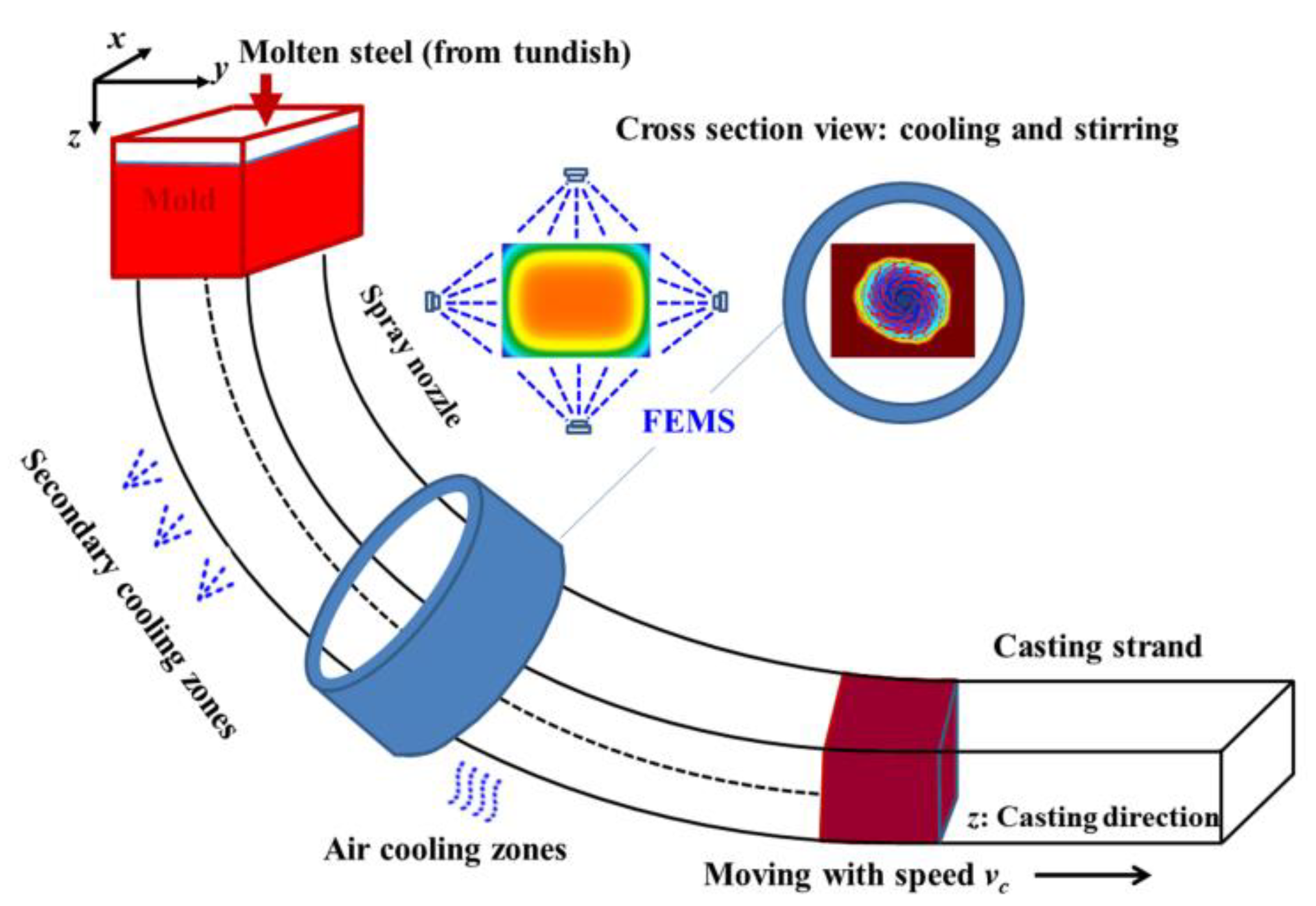
The continuous casting process is schematically shown in
Figure 1. In the process, molten steel is poured into the water-cooled copper mold from a tundish, where the initial solidified shell forms, which involves solidifying the molten steel inside. After passing through the mold, the shell enclosing the molten steel moves down into the secondary cooling zones (SCZ), where further cooling takes place by water sprays from nozzles, and the shell grows increasingly. On exit from the SCZ, the strand cools off by radiation in the air and finishes the solidification gradually. Finally, the strand is cut into segments of fixed length, and transported for rolling. During the process, secondary cooling is vital for temperature distribution and greatly influences the strand quality. In addition, to further improve the strand quality, electromagnetic stirring is commonly used, including mold electromagnetic stirring (MEMS), secondary cooling electromagnetic stirring (SEMS) and final electromagnetic stirring (FEMS). Among these, FEMS especially is supposed to be the key to improving the central quality of products, such as central segregation, porosity and shrinkage, etc. [
1].
For optimal control of secondary cooling and final electromagnetic stirring, the heat transfer model is fundamental to calculate the solidification states inside and outside. In recent years, much research has been carried out well into the heat transfer model [
2,
3,
4,
5,
6,
7]. Among these studies, most of the developed models are two-dimensional [
8] or three dimensional but offline [
9], and the steady models are applied to optimize the process parameters [
10,
11], while real-time transient ones are used for online dynamic control [
12,
13]. However, for more precise control, the model is supposed to be three dimensional and real-time. In particular, during the initial casting stage and final casting stage, the heat transfer along the casting direction is too obviously near the bottom surface or top surface to be ignored.
Conventionally, secondary cooling and FEMS are treated as two independent technologies without considering their interaction, and their parameters are generally optimized separately [
14,
15,
16]. The optimization depends on conventional optimization algorithms and plant trials. Beyond optimization, dynamic control of secondary cooling and electromagnetic stirring further benefits the quality of the stability. Dynamic control can reduce the fluctuation of solidification states during transient situations [
8,
12,
17]. In practice, due to the conflicts of multiple technologies and fluctuations under static control, the actual quality may not be the best. In 2020, Ji et al. [
18] presented a coordinated optimal control strategy based on a multiobjective particle swarm optimization (MOPSO) algorithm (our previous work), which mainly focuses on the optimization algorithm and is not precise enough in model form and not practical enough regarding metallurgical knowledge.
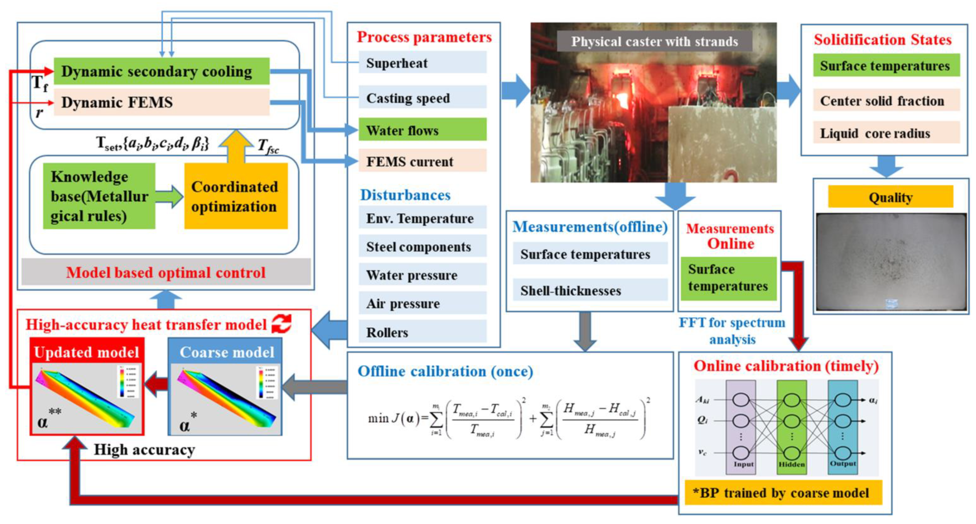
Therefore, in this paper, aiming at improving and stabilizing the product quality of steels and considering the conflicting multi-objectives, a coordinated optimization and dynamic control system was developed, and it was based on a high-accuracy three dimensional real-time heat transfer model for all stages of the continuous casting process. Firstly, a three dimensional real-time heat transfer model was established as the digital twin; for high accuracy, it was calibrated offline and online by measurements of surface temperatures and shell thicknesses. Secondly, according to metallurgical rules, cooling and stirring were coordinated and optimized based on a high-accuracy model and the chaos particle swarm optimization algorithm. Thirdly, cooling and stirring were further dynamically controlled for quality stability. Finally, the optimal control system was applied to a bloom caster, which greatly improved the product quality.
3. Digital Twin for Heat Transfer Process
3.1. 3D Real-Time Model for All Stages
The heat transfer process for continuous casting of steel can be generally simplified as a “solid” heat transport problem under two assumptions: (1) increasing heat conduction induced by the flow of non-solid steel can be taken into account by an increased effective thermal conductivity; (2) the latent heat released during solidification can be considered in equivalent specific heat. The governing equation then takes the following form in the follow-up coordinate system:
where
T is the temperature [°C] and
ρ is the density of the steel;
ceff = d
H/d
T, as
ceff is the equivalent specific heat, and
H is the enthalpy;
keff = fsks + m(1
− fs)kl, as
keff is the effective thermal conductivity,
fs is the solid fraction and
ks and
kl are, respectively, the thermal conductivity of the solid phase and liquid phase; and, significantly,
m indicates the convection intensity of the non-solid part. Properties including
ρ,
H,
fs,
ks and
kl are assumed to be functions of
T and of the steel compositions. For carbon and low-alloy steels, they can be calculated by our specially designed algorithm based on the pseudo-binary phase diagram [
19]; others can be obtained by software JMatPro (Sente Software Ltd., Guildford, UK). In Equation (1), for simplification, the shrinkage is not considered.
In the model, the casting strand is divided into a queue of slices with height
dz. Considering the symmetry, only one quarter of the cross section is selected to be the calculation domain. The initial condition of each slice is assumed to be the casting temperature:
For the steady casting stage, which takes up most of the casting time, boundary conditions are specified as follows:
- (1)
In the mold [
20]:
where
q is boundary heat flux,
t is the dwell time of the slice in the mold, and
A and
B are machine-dependent parameters.
- (2)
In the secondary cooling zones (SCZ), water cooling and thermal radiation have been considered:
where
q is the boundary heat flux,
h is the heat transfer coefficient,
ε is the emissivity of the strand surface,
σ is the Stefan–Boltzmann constant,
Tw is the water temperature and
Ta is the ambient air temperature. In SCZ, we set
ε = 0.85.
There are two kinds of sprays in different secondary cooling zones: one is the water spray, and the other is the air-mist sprays, and the heat transfer coefficients for them are respectively expressed as Equations (5) [
21] and (6) [
22].
where
wi is the water flow density (L/m
2/s) of cooling zone
i, and
αi is the machine-dependent parameter for zone
i.
- (3)
In the air cooling zone (ACZ), thermal radiation has been considered:
where
εa is the emissivity of the strand surface in ACZ.
For the initial casting stage and the final stage, there are additional conditions. Firstly, during the initial casting stage, for the dummy bar, the initial condition for extra slices of the dummy bar is T(x,y,z,0) = Te, where Te is room temperature, and the flux of surfaces, except its top surface and symmetric surfaces, are set to be radiative, with emissivity εb = 0.7, In the mold, T(x,y,z,0) = Tc. Furthermore, if we are considering the mold cooling during the fulfilling process at the very beginning of the initial stage, the transient short-time filling process can be treated as a moving process equivalent to that of the heat transfer. Secondly, during the final casting stage, when the tundish stops pouring the top surface of the strand then moves together with the entire strand, until it moves out of the calculation domain. The final casting stage lasts several minutes. In this stage, the boundary condition of the strand top surface changes to being radiative, with emissivity εu = 0.7.
Equations (1)–(7) plus additional conditions define the heat transfer model of continuous casting. The partial differential equation model can be discretized using the finite volume method (FVM) and solved using the alternative direction implicit (ADI) algorithm [
22]. In the FVM-ADI algorithm, the heat transfer model is discretized to difference equations by the integration of the finite volume of each node in the slice from
t to
t + Δ
t, as Equation (8). For real-time, non-uniform grids and variable time steps are adopted and improved for greatly reducing the number of nodes in the 3D calculation domain [
22,
23]. Moreover, the heat transfer in the
z direction can be treated as the source item. The newly developed heat transfer model is called Neucast-3D, while the former 2D one is called Neucast-2D.
where
w,
e,
s,
n, d, and
u are the interfaces of neighbor volumes and Δ
t is the time step.
3.3. Positive Online Calibration
Beyond offline calibration, online calibration is required for keeping the high accuracy of the digital twin model, since the machine-dependent parameters may change due to disturbances such as water temperature, water pressure, and so on. Therefore, a specially designed positive online calibration method [
25] was developed, which is based on reliable online surface temperature measurements with a range of 800–1200 °C and stability within ±5 °C [
26,
27].
The online calibration method contains two related parts, as shown in
Figure 3: the spectrum analysis conducted in the physical world and the prediction functions generated in the digital world.
In the physical world, in order to obtain the transfer matrix from water flows to temperatures, extra water flows in sine-wave form are positively applied to excite the temperature responses for a limited period lasting for several minutes only each time (for example, 200 s for the billet caster or 1000 s for the bloom caster). The different cooling zones in the spectra are calculated separately, using fast Fourier transform (FFT) from the temperature responses, while the temperature responses are excited by extra water flows as inputs in sine-wave form. These extra water flows are designed with different frequencies for different cooling zones, so that their responses can be distinguished in the spectrum. For each cooling zone, the characteristic amplitude of each spectrum is related to machine-dependent parameters; more exactly, it is almost directly related to the corresponding αi. During the spectrum analysis, there are two requirements for temperature measurements. Firstly, the amplitude of the interfered part of the noise spectrum’s should be less than 0.2 °C to ensure the signal-to-noise-ratio (SNR, ≥10) requirement. Secondly, the maximum frequency of the main part of the noise spectrum is below the minimum frequency of input signals (for example, 1/16 Hz for the billet or 1/40 Hz for the bloom).
In the digital world, the prediction functions take characteristic amplitudes as inputs to calculate αis. In this paper, each of the prediction functions, mapping the characteristic amplitude Aki to αi, is established based on a BP network, while the BP network is trained by the dataset {<Qi, vc, Aki, αi>}, where Qi is the water flow of the secondary cooling zone i, and vc is the casting speed. Each BP network is composed of three inputs, five hidden layers, one output layer, and one output, and the activation function is sigmoid. The BP network establishes a functional relationship between αi and <Qi, vc, Aki>. As for each <Qi, vc, Aki, αi>, it is generated by model simulation with extra sine-wave inputs. In this way, αis can be updated online.
In the studied bloom caster, there are four sections in the SCZ. For each BP neural network, 1232 data sets were used for data training, where the discrete variables Qi, vc and αi for interpolation were, respectively, eleven levels, seven levels and sixteen levels, as they were uniformly distributed in their own range.
Author Contributions
Conceptualization, J.Y. and Z.J.; methodology, J.Y.; validation, J.Y. and W.L.; writing—original draft preparation, J.Y. and Z.J.; writing—review and editing, J.Y.; project administration, Z.X.; funding acquisition, J.Y. All authors have read and agreed to the published version of the manuscript.
Funding
This research was funded by the National Natural Science Foundation of China, grant number U21A20117, 52074081, 52074085, and 61703084. The APC was funded by U21A20117.
Data Availability Statement
The data presented in this study are available on request from the corresponding author. The data are not publicly available due to privacy.
Acknowledgments
The authors gratefully thank the financial support of the National Natural Science Foundation of China Grants U21A20117, 52074081, 52074085, and 61703084, and the research support of Nanjing Iron & Steel Cooperation (NISCO).
Conflicts of Interest
The authors declare no conflict of interest. The funders had no role in the design of the study; in the collection, analyses, or interpretation of data; in the writing of the manuscript, or in the decision to publish the results.
Nomenclature
| T | Temperature | G | Transfer function matrix |
| ρ | Density | gij | Transfer function |
| H | Enthalpy | Kij | Static gain for transfer function |
| fs | Solid fraction | tij | inertia time constant |
| k | Thermal conductivity | vc | Casting speed |
| ceff | Equivalent specific heat | ΔTw | Mold in-out temperature difference |
| x,y,z | Coordinates | Aki | Spectra amplitude |
| Tc | Casting temperature | vei | Effective casting speed |
| A,B | Mold cooling parameters | ΔTei | Effective superheat |
| αi | Cooling parameter for Zone i | ΔTstd | Standard superheat |
| m | Convection-related parameter | Bm | Magnetic induction intensity |
| ε | Emissivity | cw | Water specific heat |
| Q | Water flow | lmeff | Effective mold length |
| q | Boundary heat flux | | |
| h | Heat transfer coefficient | Subscripts | |
| Hmea,j | Measured shell thickness | i | Zone number in SCZ |
| Hcal,j | Calculated shell thickness | a | Air cooling zone |
| Tmea,i | Measured surface temperature | w | water |
| Tcal,i | Calculated surface temperature | ij Zone j | affects Zone i |
| Qw | Water flow in mold | i = 1,2,3,…,N | Specific zone number |
References
- Mao, B.; Zhang, G.; Li, A. Theory and Technology of Electromagnetic Stirring for Continuous Casting; Metallurgical Industry Press: Beijing, China, 2012. [Google Scholar]
- Ji, C.; Deng, S.; Guan, R.; Zhu, M. Real-time heat transfer model based on distributed thermophysical property calculation for the continuous casting process. Steel Res. Int. 2019, 90, 1800476. [Google Scholar] [CrossRef]
- Yunwei, H.; Mujun, L.; Dengfu, C.; Kai, T.; Huamei, D.; Pei, X. Effect of hot water vapor on strand surface temperature measurement in steel continuous casting. Int. J. Therm. Sci. 2019, 138, 467–479. [Google Scholar]
- Ma, J.; Xie, Z.; Jia, G. Applying of Real-time Heat Transfer and Solidification Model on the Dynamic Control System of Billet Continuous Casting. ISIJ Int. 2008, 48, 1722–1727. [Google Scholar] [CrossRef]
- Louhenkilpi, S.; Mäkinen, M.; Vapalahti, S.; Räisänen, T.; Laine, J. 3D steady state and transient simulation tools for heat transfer and solidification in continuous casting. Mater. Sci. Eng. A 2005, 413, 135–138. [Google Scholar] [CrossRef]
- Blazek, K.; Moravec, R.; Zheng, K.; Lowry, M.; Gregurich, N.; Flick, G. New pseudo-3D dynamic secondary cooling model implementation and results at arcelormittal burns harbor. Iron Steel Technol. 2016, 13, 78–85. [Google Scholar]
- Thomas, B.G. Review on Modeling and Simulation of Continuous Casting. Steel Res. Int. 2017, 89, 1700312. [Google Scholar] [CrossRef]
- Zhao, Y.; Chen, D.F.; Long, M.J.; Shen, J.L.; Qin, R.S. Two-dimensional heat transfer model for secondary cooling of continuously cast beam blanks. Ironmak. Steelmak. 2013, 41, 377–386. [Google Scholar] [CrossRef]
- Hardin, R.; Du, P.; Beckermann, C. Three-dimensional Simulation of Heat Transfer and Stresses in a Steel Slab Caster. In Proceedings of the 4th International Conference on Modeling and Simulation of Metallurgical Processes in Steelmaking, Paper No. STSI-71, Steel Institute VDEh, Düsseldorf, Germany, 27 June–1 July 2011; pp. 1–6. [Google Scholar]
- Mauder, T.; Stetina, J. Optimization of the secondary cooling in a continuous casting process with different slab cross-sections. Mater. Tehnol. 2014, 48, 521–524. [Google Scholar]
- Zhai, Y.Y.; Li, Y.; Ao, Z.G. Optimization of continuous casting secondary cooling based on an enhanced multi-objective genetic algorithm. J. Northeast. Univ. 2019, 40, 658–662. [Google Scholar]
- Ma, J.C.; Lu, C.S.; Yan, Y.T.; Chen, L.Y. Design and application of dynamic secondary cooling control based on real time heat transfer model for continuous casting. Int. J. Cast Met. Res. 2013, 27, 135–140. [Google Scholar] [CrossRef]
- Petrus, B.; Zheng, K.; Zhou, X.; Thomas, B.G.; Bentsman, J. Real-time, model-based spray-cooling control system for steel continuous casting. Metall. Mater. Trans. B Vol. 2011, 42, 87–103. [Google Scholar] [CrossRef]
- Xiao, C.; Zhang, J.-M.; Luo, Y.-Z.; Wei, X.-D.; Wu, L.; Wang, S.-X. Control of Macrosegregation Behavior by Applying Final Electromagnetic Stirring for Continuously Cast High Carbon Steel Billet. J. Iron Steel Res. Int. 2013, 20, 13–20. [Google Scholar] [CrossRef]
- Su, W.; Wang, W.-L.; Luo, S.; Jiang, D.-B.; Zhu, M.-Y. Heat Transfer and Central Segregation of Continuously Cast High Carbon Steel Billet. J. Iron Steel Res. Int. 2014, 21, 565–574. [Google Scholar] [CrossRef]
- Luo, S.; Piao, F.Y.; Jiang, D.D.; Wang, W.L.; Zhu, M.Y. Numerical Simulation and Experimental Study of F-EMS for Continuously Cast Billet of High Carbon Steel. J. Iron Steel Res. Int. 2014, 21, 51–55. [Google Scholar] [CrossRef]
- Yu, Y.; Luo, X.; Zhang, H.; Zhang, Q. Dynamic optimization method of secondary cooling water quantity in continuous casting based on three-dimensional transient nonlinear convective heat transfer equation. Appl. Therm. Eng. 2019, 160, 113988. [Google Scholar] [CrossRef]
- Wu, D.S.; Ji, Z.P.; Yang, J.; Gao, H.W.; Yu, J.H.; Ju, Z.J. Coordinated optimal control of secondary cooling and final elec-tromagnetic stirring for continuous casting billets. J. Control Sci. Eng. 2020, 2020, 1–9. [Google Scholar] [CrossRef]
- Xie, Z.; Yang, J. Calculation of Solidification-Related Thermophysical Properties of Steels Based on Fe-C Pseudobinary Phase Diagram. Steel Res. Int. 2014, 86, 766–774. [Google Scholar] [CrossRef]
- Savage, J.; Pritchard, W. The problem of rupture of the billet in the continuous casting of steel. J. Iron Steel Inst. 1954, 178, 269–277. [Google Scholar]
- Nozaki, T.; Matsuno, J.-I.; Murata, K.; Ooi, H.; Kodama, M. A Secondary Cooling Pattern for Preventing Surface Cracks of Continuous Casting Slab. Trans. Iron Steel Inst. Jpn. 1978, 18, 330–338. [Google Scholar] [CrossRef]
- Yang, J.; Xie, Z.; Ji, Z.; Meng, H. Real-time Heat Transfer Model Based on Variable Non-uniform Grid for Dynamic Control of Continuous Casting Billets. ISIJ Int. 2014, 54, 328–335. [Google Scholar] [CrossRef]
- Yang, J.; Xie, Z.; Meng, H.J.; Liu, W.H.; Ji, Z.P. Multiple time steps optimization for real-time heat transfer model of continuous casting billets. Int. J. Heat Mass Tran. 2014, 76, 492–498. [Google Scholar] [CrossRef]
- Meng, J.Y.H.J.; Ji, Z.P.; Xie, Z. Parameter identification of heat transfer model for continuous casting billets based on chaos particle swarm optimization. J. Northeast. Univ. (Nat. Sci.) 2014, 35, 613–616. (In Chinese) [Google Scholar]
- Yang, J.; Xie, Z.; Hu, Z.W.; Wang, J.J.; Wei, W. Positive Online Calibration of Heat Transfer Model for Continuous Casting of Steel Based on Surface Temperature Measurement. 2022. Available online: https://ssrn.com/abstract=4272505 (accessed on 9 November 2022).
- Peng, W.; Zhi, X.; Zhenwei, H. Study on the multi-wavelength emissivity of GCr15 steel and its application on temperature measurement for continuous casting billets. Int. J. Thermophys. 2016, 37, 129. [Google Scholar]
- Peng, W.; Zhenwei, H.; Zhi, X.; Ming, Y. A new experimental apparatus for emissivity measurements of steel and the application of multi-wavelength thermometry to continuous casting billets. Rev. Sci. Instrum. 2018, 89, 054903. [Google Scholar]
- Gan, Y. Practical Manual of Modern Continuous Casting of Steel; Metallurgical Industry Press: Beijing, China, 2010. [Google Scholar]
- Cai, K. Quality Control of Continuous Casting Slabs; Metallurgy Industry Press: Beijing, China, 2010. [Google Scholar]
- Wang, F.-S.; Juang, W.-S.; Chan, C.-T. Optimal tuning of pid controllers for single and cascade control loops. Chem. Eng. Commun. 1995, 132, 15–34. [Google Scholar] [CrossRef]
Figure 1.
Continuous casting process.
Figure 2.
Intelligent optimal control strategy based on high-accuracy model.
Figure 3.
Online calibration method.
Figure 4.
Calculated time-variant temperature field. (a) Initial stage; (b) after 4000 s; (c) final stage.
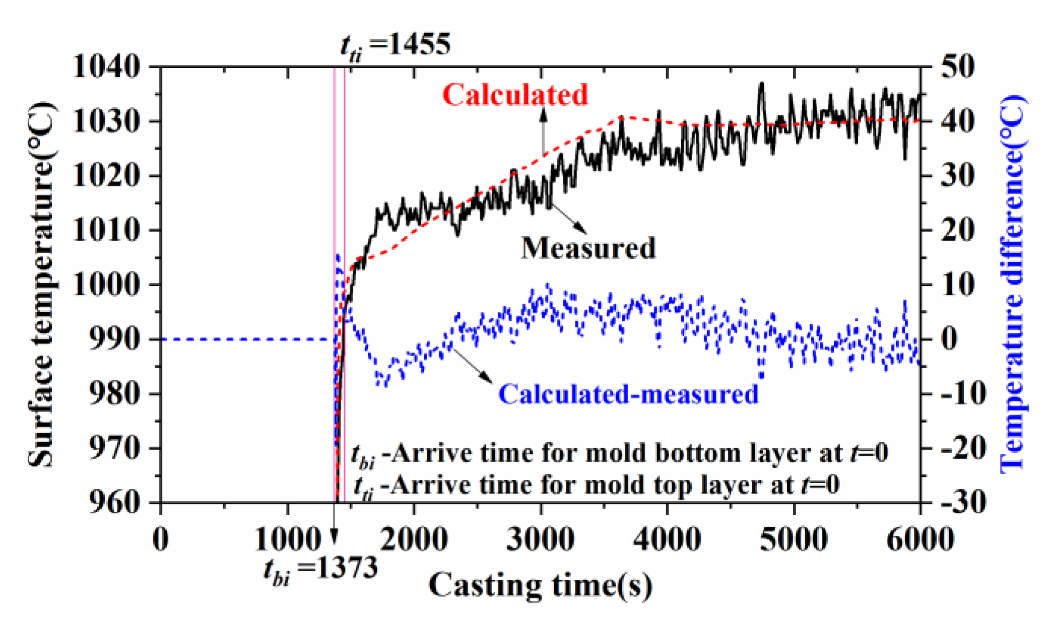
Figure 5.
Calculated surface-center temperatures vs. measurements at z = 12 m (distance from meniscus).
Figure 6.
High-temperature strength of steels.
Figure 7.
Viscosity variation with solid fraction.
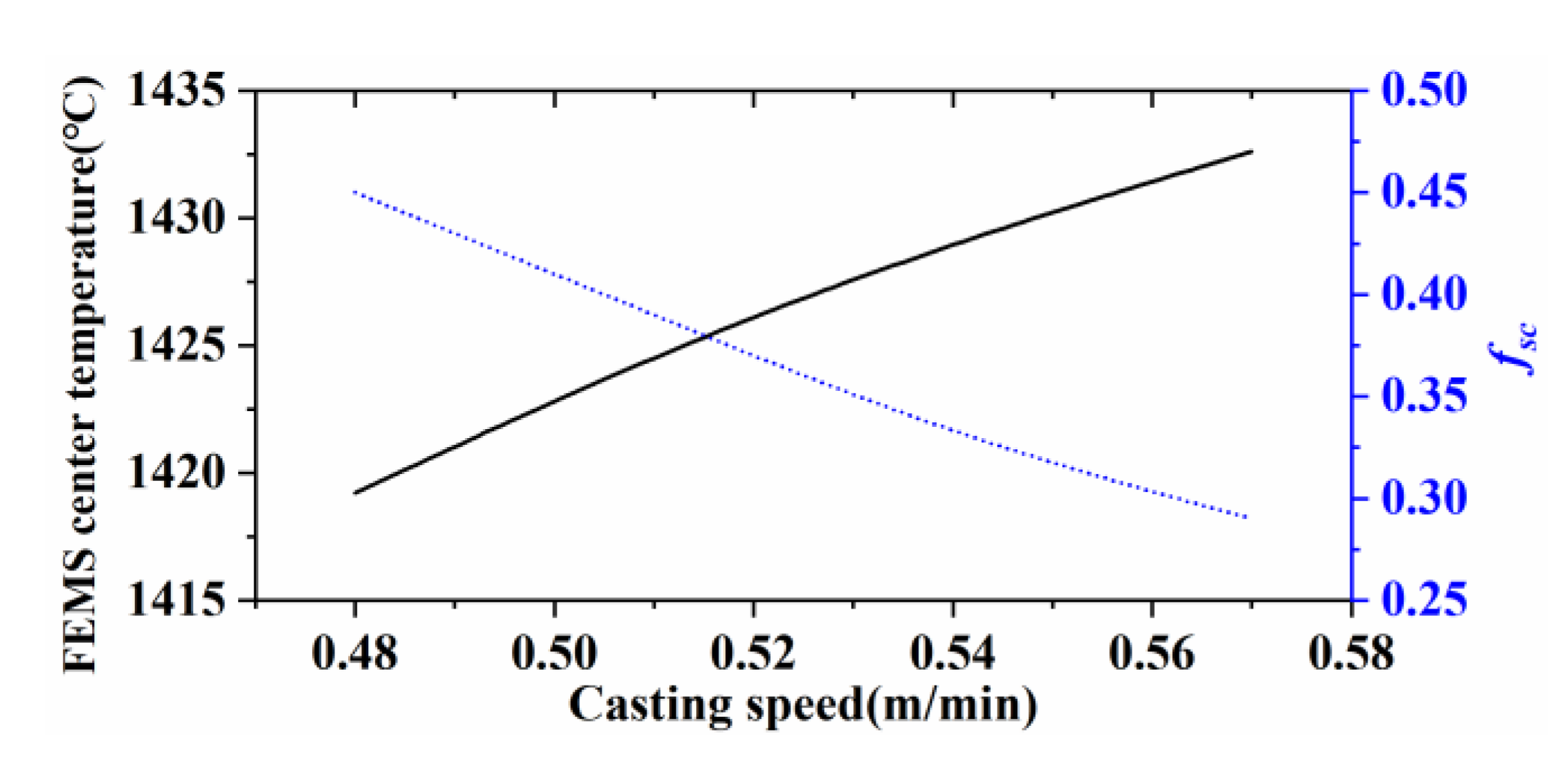
Figure 8.
FEMS center temperature under different casting speeds.
Figure 9.
Measuring method and device for FEMS.
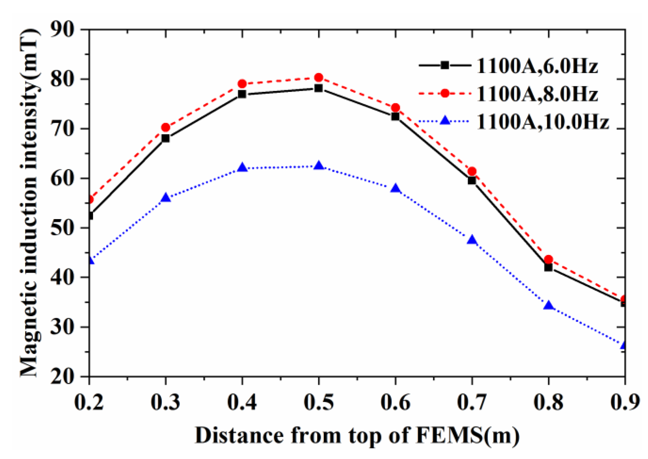
Figure 10.
Measured magnetic induction intensity.
Figure 11.
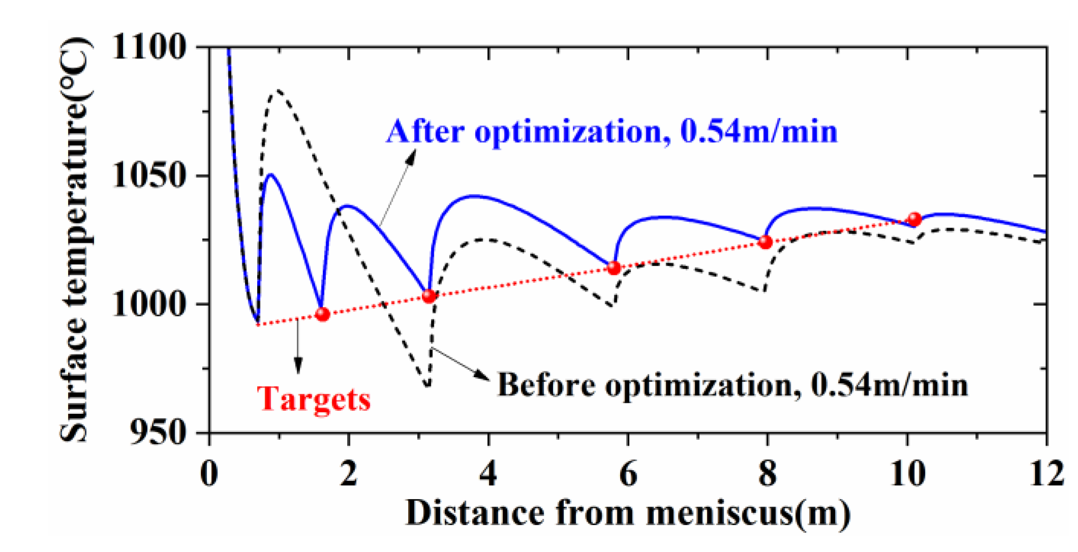
Temperatures before and after optimization.
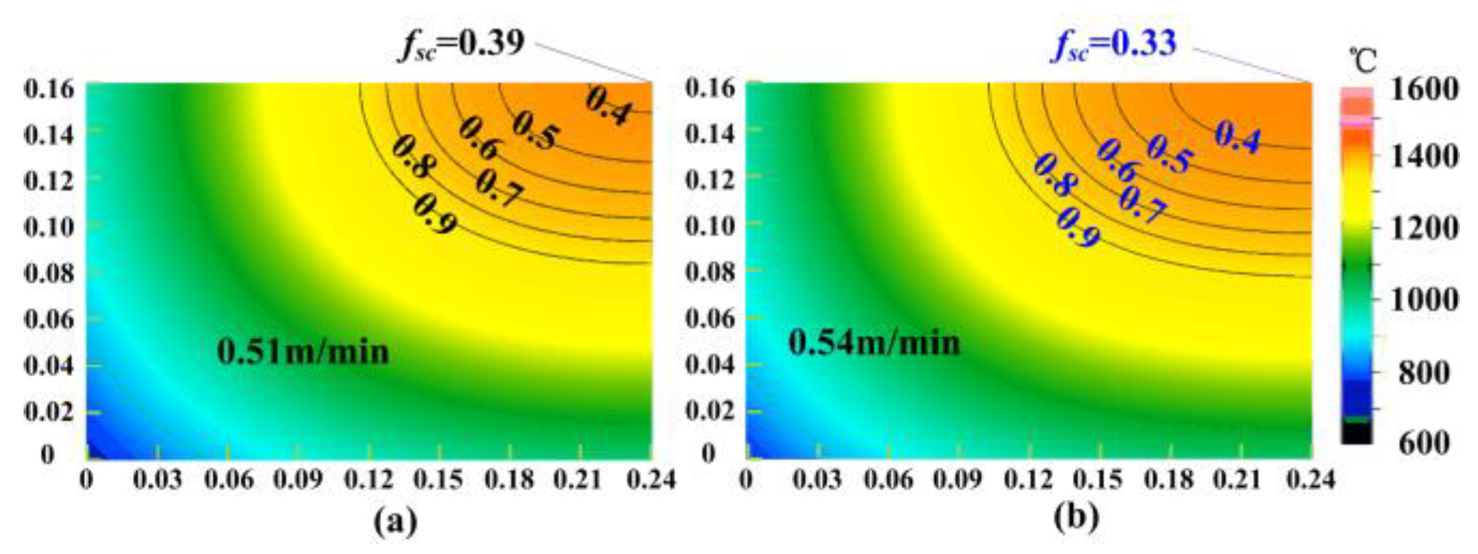
Figure 12.
Solid fraction at the middle of FEMS: (a) before optimization; (b) after optimization.
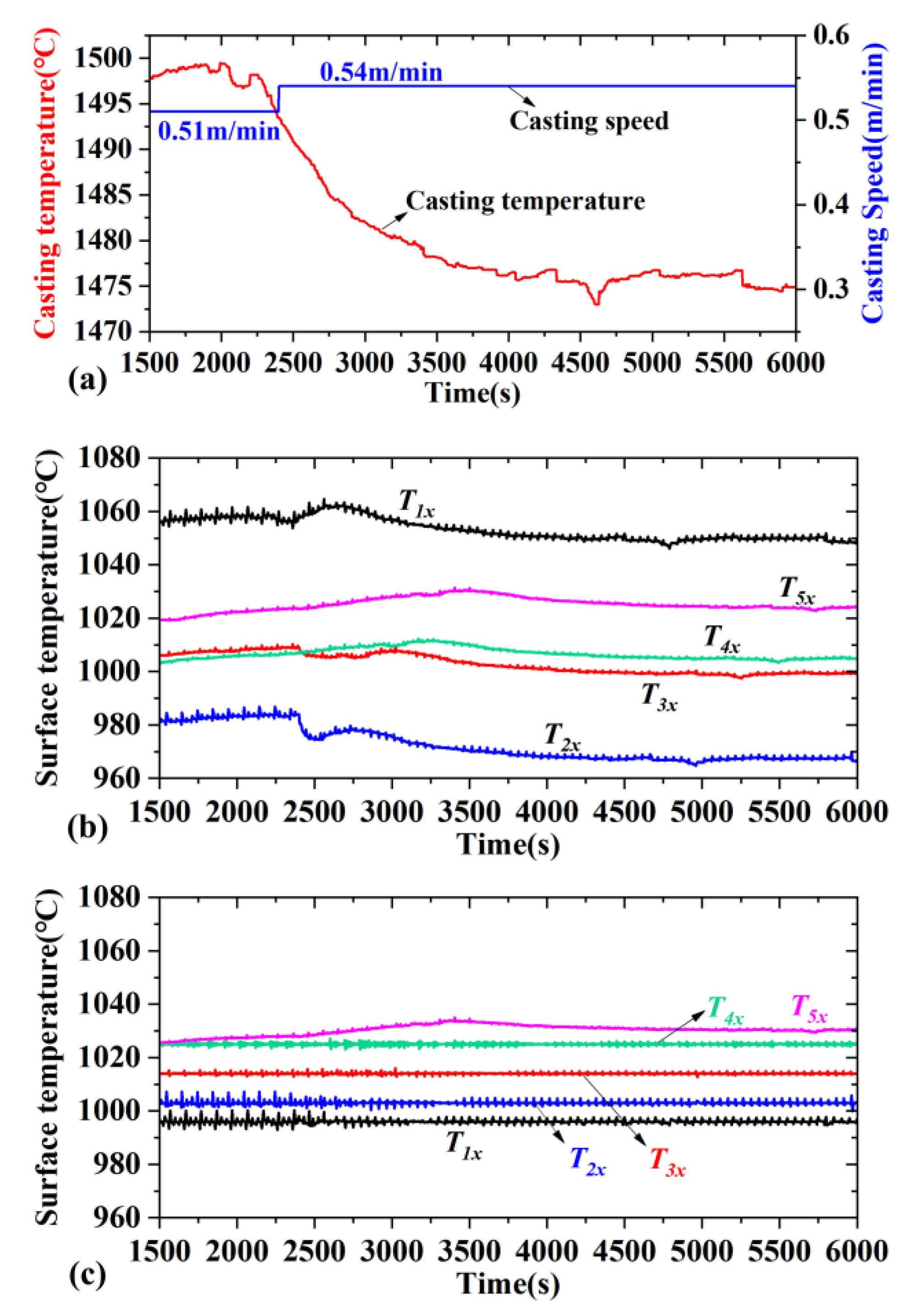
Figure 13.
Surface center temperatures at the end of different zones: (a) casting conditions; (b) surface temperatures before optimization; (c) surface temperatures after optimization.
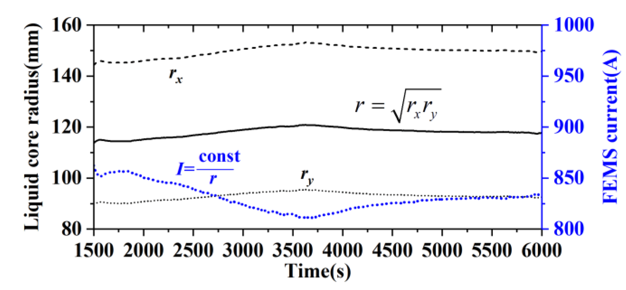
Figure 14.
Dynamic control of FEMS current.
Figure 15.
Macrographs: (a) before optimal control; (b) after optimal control.
Table 1.
Key temperatures for different steels.
| Temperature | GCr15 (°C) | 45# (°C) | 20# (°C) |
|---|
| A3 | 883 * | 770 | 835 |
| (fs = 0.35) | 1428 | 1471 | 1505 |
Table 2.
Components of steels.
| Element | GCr15 (%wt) | 45# (%wt) | 20# (%wt) |
|---|
| C | 0.974 | 0.46 | 0.21 |
| Si | 0.226 | 0.26 | 0.29 |
| Mn | 0.316 | 0.680 | 0.50 |
| P | 0.011 | 0.035 | 0.011 |
| S | 0.002 | 0.025 | 0.006 |
| Cr | 1.454 | 0.046 | - |
| Mo | 0.005 | - | - |
| Ni | 0.045 | 0.04 | 0.04 |
| Cu | 0.063 | 0.16 | - |
Table 3.
Target temperatures for GCr15.
| Zone | Ttarget | Tset | Zone | Ttarget | Tset |
|---|
| 1IO | 996 | 996 | 1N | 1006 | 1006 |
| 2IO | 1003 | 1003 | 2N | 1011 | 1011 |
| 3IO | 1014 | 1014 | 3N | 1019 | 1019 |
| 4IO | 1024 | 1024 | 4N | 1026 | 1026 |
| 5IO | 1033 | 1030 | 5N | 1033 | 994 |
| FEMS center | 1428 | 1429 | | | |
Table 4.
Optimized water table for GCr15.
| Zone and Side | Casting Speed (m/min) |
|---|
| 0.48 | 0.51 | 0.54 | 0.57 |
|---|
| 1IO | 42.15 | 45.95 | 49.85 | 53.87 |
| 1N | 26.37 | 28.82 | 31.38 | 34.07 |
| 2IO | 14.35 | 15.25 | 16.15 | 17.04 |
| 2N | 8.92 | 9.56 | 10.19 | 10.81 |
| 3IO | 10.11 | 11.18 | 12.24 | 13.31 |
| 3N | 4.37 | 5.29 | 6.16 | 7.00 |
| 4IO | 2.39 | 3.16 | 3.88 | 4.55 |
| 4N | 0 | 0 | 0.14 | 0.78 |
| 5IO | 0 | 0 | 0 | 0 |
| 5N | 0 | 0 | 0 | 0 |
Table 5.
Geometric parameters of studied caster.
| Parameter | Value |
|---|
| Size (mm2) | 320 × 480 |
| Radius (m) | 12 |
| Mold length (m) | 0.8 (effective length: 0.7) |
| Lengths of SCZ (m) | [0.93,1.52,2.65,2.17,2.14] |
| FEMS position (m) | 12.2 (fixed) |
Table 6.
Water table for GCr15 before optimization.
| Zone and Side | Casting Speed (m/min) |
|---|
| 0.48 | 0.51 | 0.54 | 0.57 |
|---|
| 1IO | 28.8 | 28.8 | 28.8 | 28.8 |
| 1N | 16.8 | 16.8 | 16.8 | 16.8 |
| 2IO | 18.7 | 20.1 | 21.5 | 22.9 |
| 2N | 12.6 | 13.6 | 14.6 | 15.6 |
| 3IO | 12.4 | 13.4 | 14.4 | 15.4 |
| 3N | 8.2 | 8.9 | 9.6 | 10.3 |
| 4IO | 6 | 6 | 6 | 6 |
| 4N | 6 | 6 | 6 | 6 |
| 5IO/5N | 0 | 0 | 0 | 0 |
Table 7.
Calibrated parameters of model.
| Parameters | Before Calibration | Calibrated Value |
|---|
| A (W/m2) | 2.68 × 10⁶ | 1.546 × 10⁶ |
| B (W/(m2·s1/2)) | 3.35 × 10⁵ | 1.067 × 10⁵ |
| α1 | 4 | 3.788 |
| α2 | 1 | 1.043 |
| α3 | 1 | 1.043 |
| α4 | 1 | 1.043 |
| α5 | 1 | 1.043 |
| εa | 0.85 | 0.759 |
| m | 1 | 2.786 |
Table 8.
Optimized coefficients for GCr15.
| Zone | ai | bi | ci | di | βi | Tset,i |
|---|
| 1IO | 0 | 74.28 | 52.19 | 0.00 | 0.00698 | 996 |
| 1N | 0 | 53.75 | 29.11 | 0.00 | 0.00724 | 1006 |
| 2IO | 0 | −0.01 | 29.90 | 0.00 | 0.00389 | 1003 |
| 2N | 0 | 4.18 | 16.60 | 0.00 | 0.00366 | 1011 |
| 3IO | 0 | 25.23 | 9.00 | 0.00 | 0.00507 | 1014 |
| 3N | 0 | 34.91 | −7.53 | 0.00 | 0.00524 | 1020 |
| 4IO | 37.85 | −7.19 | −0.12 | 0.00 | 0.00853 | 1025 |
| 4N | 46.14 | −32.58 | 4.74 | 0.00 | 0.07582 | 1024 |
| 5IO | 0 | 0 | 0 | 0 | 0 | - |
| 5N | 0 | 0 | 0 | 0 | 0 | - |
| Disclaimer/Publisher’s Note: The statements, opinions and data contained in all publications are solely those of the individual author(s) and contributor(s) and not of MDPI and/or the editor(s). MDPI and/or the editor(s) disclaim responsibility for any injury to people or property resulting from any ideas, methods, instructions or products referred to in the content. |
© 2023 by the authors. Licensee MDPI, Basel, Switzerland. This article is an open access article distributed under the terms and conditions of the Creative Commons Attribution (CC BY) license (https://creativecommons.org/licenses/by/4.0/).


