Measurements of Stray Magnetic Fields of Fe-Rich Amorphous Microwires Using a Scanning GMI Magnetometer

Abstract

A scanning magnetometer based on a magnetoimpedance sensor with a 1 mm spatial resolution and 10 nT sensitivity was used to study stray magnetic fields of Fe₇₄B₁₃Si₁₁C₂ amorphous ferromagnetic microwires. Spatial magnetic images and vertical component profiles of stray magnetic fields of the studied microwires were obtained in a longitudinal homogeneous magnetic field of Helmholtz coils with a strength in the range of ±600 A/m. A magnetic calculation method is suggested that allows for using the measured magnetic fields to determine the magnitude and pattern of magnetization for the microwire. Characteristic values of the microwires’ average magnetization and width of closure domains for various values of bias fields were found.

1. Introduction

Glass-coated amorphous ferromagnetic microwires fabricated via the Taylor–Ulitovsky technique have a unique combination of magnetic and mechanical properties suitable for a variety of sensor applications [1,2,3,4,5]. This well-proven method allows for manufacturing microwires with diverse compositions and a wide range of full diameters D ranging from 1 to 50 µm. Ideal Co-rich microwires with a small negative magnetostriction constant (λ_s ~ −(1–3) × 10⁻⁷) are characterized by a linear hysteresis loop with a very low coercive force, H_c ~ 4 A/m, and a small effective anisotropy field, H_a,ef ~ 80 A/m. These microwires demonstrate a significant magnetoimpedance effect (GMI) with a high GMI ratio [6,7,8,9]. Such microwires can used for the creation of a new generation of GMI sensitive miniaturized magnetometers [10,11]. These can be used for measuring homogeneous magnetic fields, e.g., vector components of the Earth’s magnetic field. Due to their small size, GMI sensors can also be used in scanning magnetometers to measure weak local magnetic fields. In [12,13,14,15], a scanning GMI magnetometer was applied to measure local magnetic fields from signs on banknotes and text characters printed on paper with a laser printer; fields were generated by weak electric currents and ion currents caused by corrosive processes. As shown in [15], a scanning GMI magnetometer is able to measure weak magnetic fields of small-size objects with a sensitivity of ~10 nT and spatial resolution of ~1 mm.

In contrast to Co-rich microwires, Fe-rich microwires have a positive magnetostriction constant that is one or two orders higher (λ_s ~ +(1–3) × 10⁻⁵) [2]. The hysteresis loop in such microwires is rectangular [16,17,18] with a characteristic reversal field of H_c ~ 80–400 A/m. It is assumed that the domain structure of Fe-rich microwires with positive magnetostriction consists of a single axial domain that is surrounded by an outer transversally magnetized shell. Moreover, small closure domains appear at the ends of the microwire, in order to reduce magnetostatic energy. As a result of the peculiar domain structure, the magnetization reversal process in the axial direction runs through the depinning and subsequent propagation of the closure domain wall along the entire microwire in one large Barkhausen jump (rapid motion of the domain wall (DW) along the microwire axis) [19,20]. This magnetization reversal occurs at some negative value of the external switching field (coercive field H₀). This effect can be used in the development of memory devices, magnetic logic units, and magnetic labels [21,22,23,24]. Single DW propagation in Fe-rich microwires is the subject of intensive research associated with methods for reproducible DW injection, control of DW propagation, and its structure [25,26,27,28,29,30]. Research on the DW structure involves the comparison of experimental findings with the results of calculation under a theoretical model [31]. In most cases, the DW structure of Fe-rich microwires is derived on the basis of indirect data (shape of the hysteresis loop, shape of the DW-induced signal) and theoretical estimations [32,33,34,35,36].

As reported before [37,38], the distribution of DW propagation begins from the ends of the microwire where the closure domains exist because of the demagnetizing field effect. The possibility of measuring stray magnetic fields from the closure domains in Fe-rich microwires was demonstrated in [39] at the liquid nitrogen boiling temperature by means of a scanning magnetometer based on an HT SQUID (high-temperature superconducting quantum interference device) and [14] at room temperature by means of a scanning GMI magnetometer.

In this work, using the scanning GMI magnetometry method, we conducted measurements of weak local magnetic fields near Fe-rich microwire segments while magnetizing them with external longitudinal fields. This allowed us to determine the magnitude and the distribution of magnetization along a microwire segment and evaluate the width of the closure domains.

2. Materials and Methods

The samples we used were segments of glass-coated amorphous Fe-rich microwires fabricated via the Taylor–Ulitovsky technique from Fe₇₄B₁₃Si₁₁C₂ alloy. The microwires had a metal core diameter of 16.8 µm and a full diameter of 27.14 µm. During the measurements, two segments of the microwire with a length of 2L 6.5 mm and 15.5 mm, were investigated.

During the research in which the scanning GMI magnetometry technique was employed, images of the stray magnetic fields of the microwire samples in a variety of external homogeneous magnetic fields were obtained. For comparison, with the use of the vibrating sample magnetometry technique [36], the hysteresis loop of a 6.5 mm microwire segment was measured.

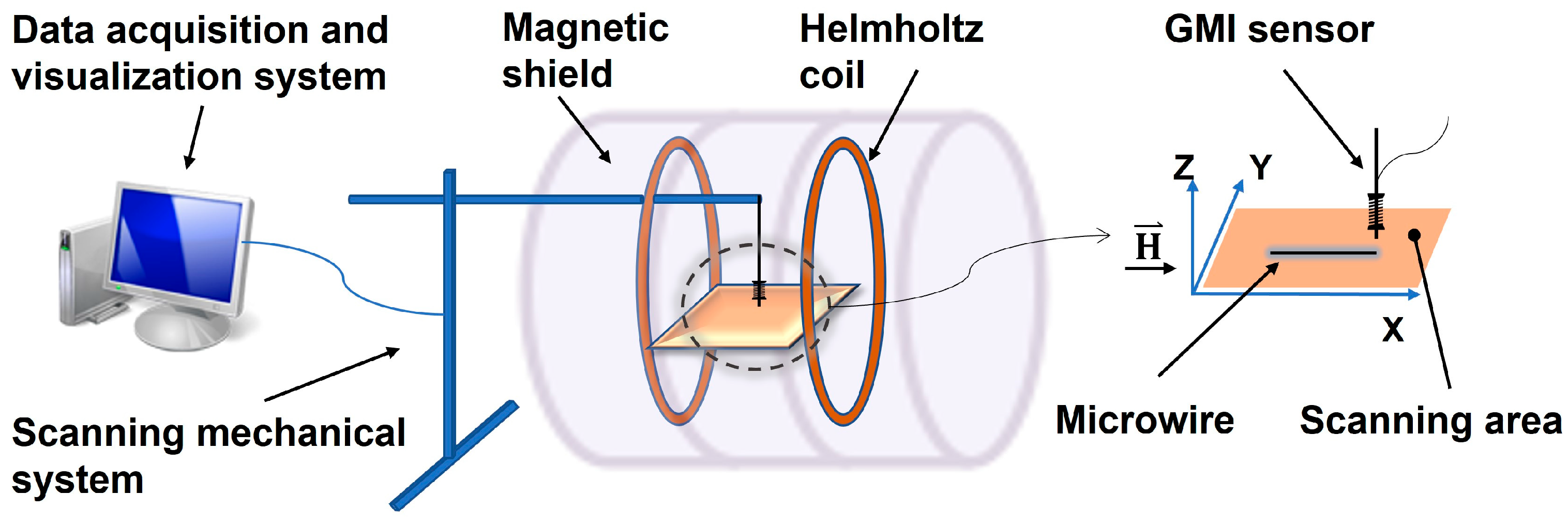
Scanning GMI Magnetometer Description

For measurements of local stray magnetic fields near Fe-rich microwire samples, a scanning GMI magnetometer was used [15], which was additionally equipped with a homogeneous magnetic field source based on Helmholtz coils (HCs). The functional setup of the upgraded GMI magnetometer is shown in Figure 1. As in the original version, the scanning magnetometer are a two-layer magnetic shield, inside which a GMI magnetometer with a miniature GMI sensor based on a Co-rich microwire and a non-magnetic mobile XYZ mechanism with a coordinate table for mounting the sample are placed. The scanning GMI magnetometer is controlled by means of a customized data acquisition and visualization system on a personal computer with specialized software. During the measurements, the miniature GMI sensor was positioned vertically, along the Z axis, at a minimal distance of Z₀ ~ 0.5 mm from the working surface of the coordinate table (X-Y plane). The microwire sample to be studied was fixed so that its centerline was parallel to the X axis. In the course of the experiments, the vertical component of the magnetic field above the sample was measured, depending on the X-Y coordinates, B_z(x, y).

For the magnetization of the microwire being studied, we used a system of additional HCs that ensured the setting of a constant homogeneous magnetic field along the X axis, B_x. The orientation chosen for the microwire, GMI sensor, and HC system (inset in Figure 1) allowed setting the magnetic field B_x to such a magnitude as to magnetize the microwire until nearly-saturated state. At the same time, the GMI sensor does not sense the external magnetic field H_x but retains high sensitivity during the measurements of the normal component of local magnetic fields, B_z(x, y), generated by the microwire magnetization. In our case, a sinusoidal current with an amplitude of 1 mA and a frequency of 4 MHz was passed through the GMI-sensor. Its sensitivity was ~10 nT, and its full dynamic range was equal to ±20 × 10³ nT. The HC system had a transfer coefficient of 600 A/m per 1 A and allowed the magnetic of ±600 A/m (to ±750 × 10³ nT).

In order to ensure attenuation of the magnetic field of the Earth and protection from 50 Hz mains magnetic interferences, the measurements were made inside a permalloy magnetic shield with the magnetic field attenuation factor of ~500.

3. Results and Discussion

In the course of the experiments using scanning GMI magnetometer, we always initially magnetized the microwire sample to the saturation state and then successively decreased the magnetizing field with a small (10 A/m) step. For each value of the applied magnetic field, we were making point-by-point measurements of the B_z (vertical) component of the stray magnetic field above the studied microwire in the scanning area of 20 × 30 mm² at a set height of Z₀ ⪞ 0.5 mm. The values of the B_z component were measured along the X axis with 0.05 mm increment, with successive displacement at 0.05 mm increments along the Y axis and recorded into a data file. Due to the low noise level of the GMI sensor, the main measurement error was within ±10 nT. The obtained magnetic data of B_z(x, y), after the processing by a special computer software, are represented as individual magnetic profiles of B_z(x) or two-dimensional colorful magnetic images.

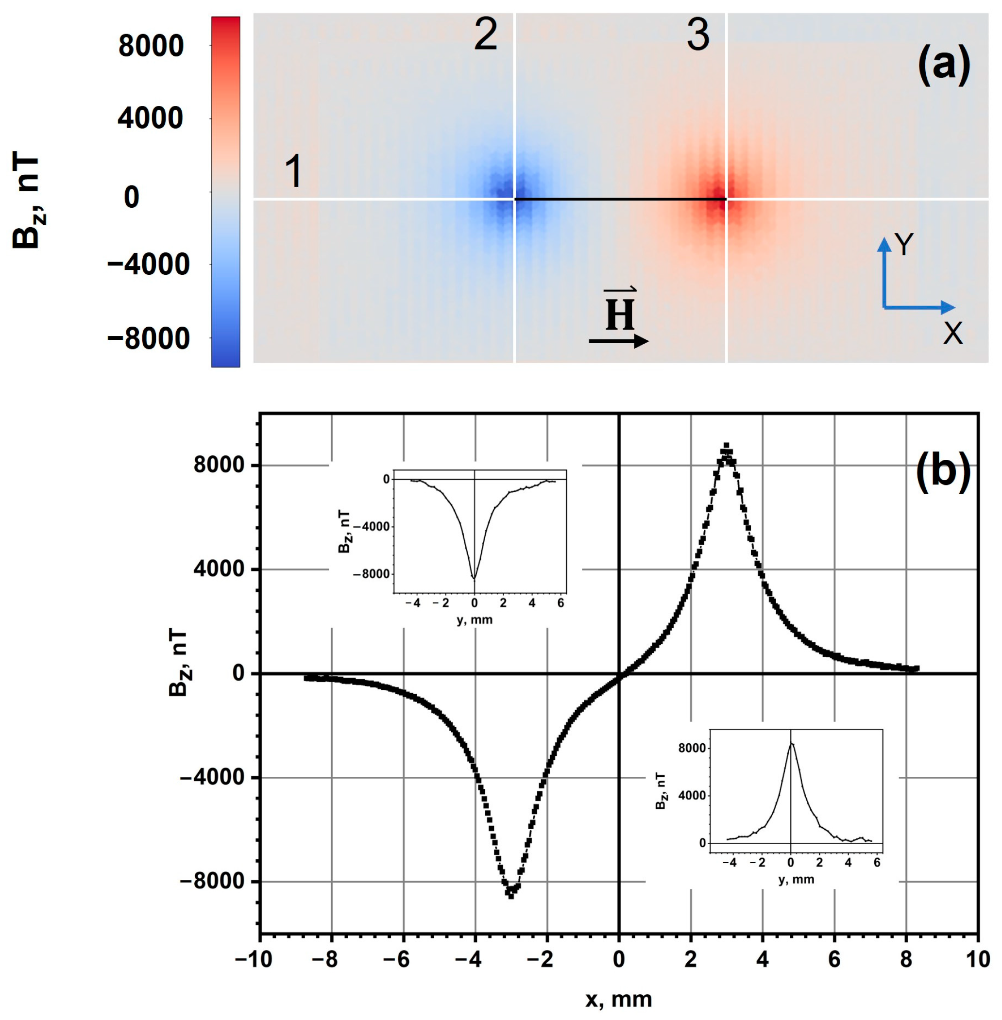
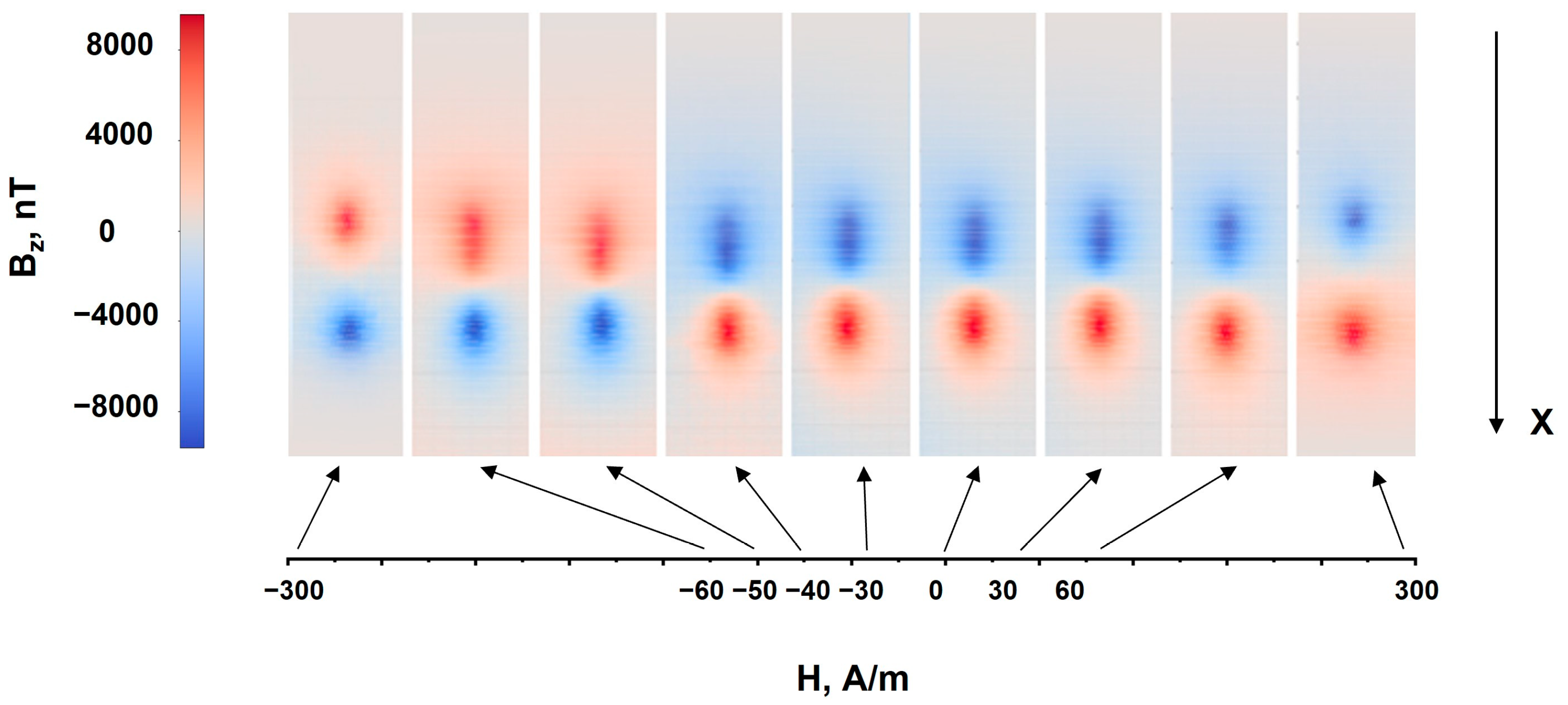
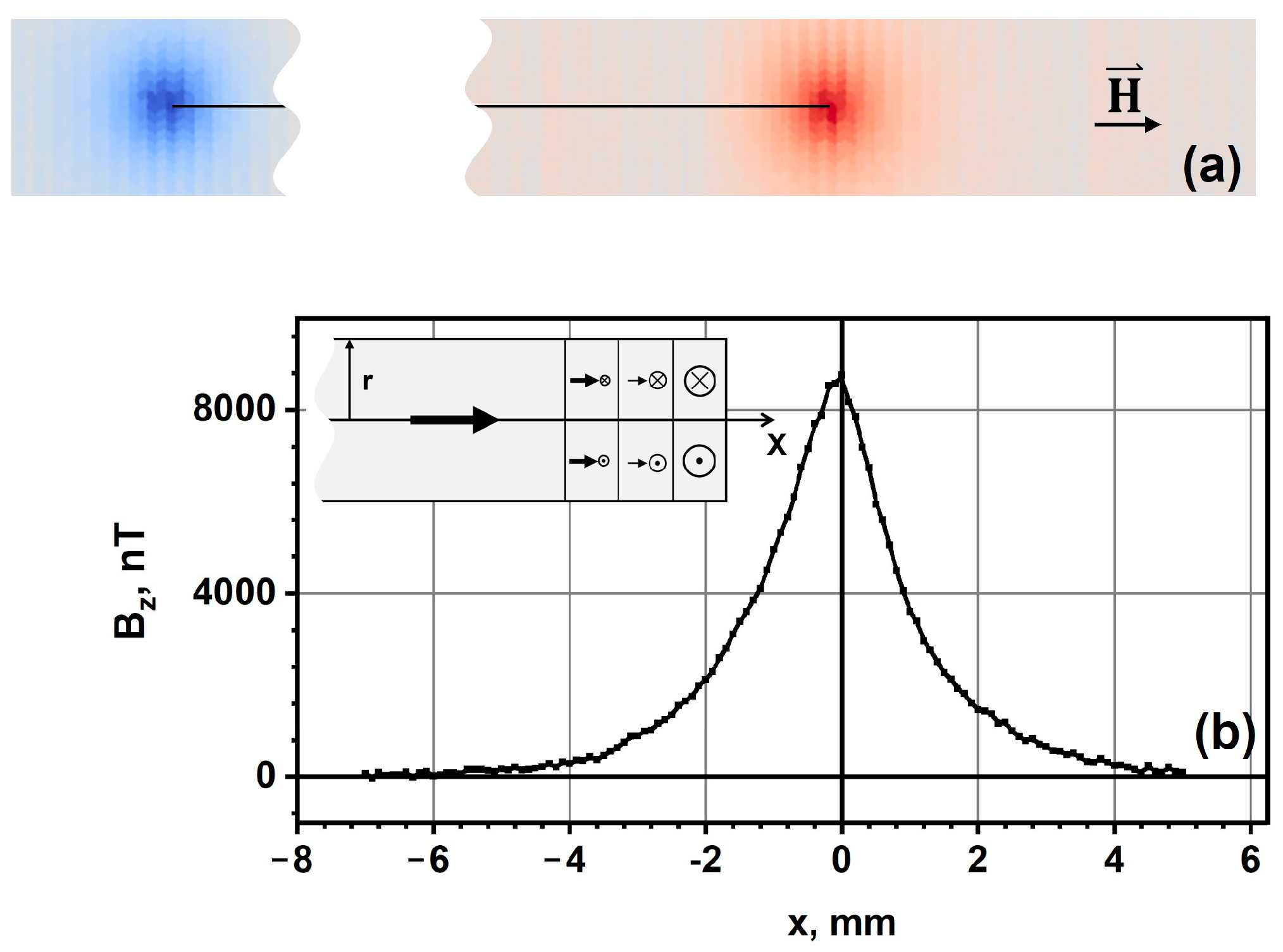
3.1. Magnetic Images of Fe-Rich Microwire Samples

Figure 2a shows a two-dimensional image of the B_z(x, y) component of the magnetic field above the 6.5 mm microwire sample (black segment in the center) measured at the height of Z₀ ⪞ 0.5 mm. This magnetic image was obtained with the influence of the HC magnetic field, 400 A/m in magnitude, directed along the microwire centerline, in which the microwire is magnetized until reaching a nearly-saturated state. In the vicinity of the microwire segment ends, in its magnetic image, two symmetrical local extremums with opposite signs were observed. This magnetic field distribution testifies that there were “magnetic charges” on the microwire segment ends. Figure 2b shows the individual magnetic profile of B_z(x), measured along the “a” axis passing parallel to the microwire’s centerline. It can be seen that the amplitude of the stray magnetic fields at the ends of segments reached the values of ±8200 nT and faded to zero, going farther from the end to a distance of x > 2L. The insets on the left and right parts of Figure 2b represent the transverse profiles of B_z(y) of the vertical component of the field, measured along the “b” and “c” axes, respectively.

Figure 3 shows a series of magnetic images of a 6.5-mm microwire depending on the magnitude of the HC longitudinal magnetic field. As follows from the presented magnetic images, at the maximum value of the bias magnetic field (+300 A/m), the positive and negative maximums of B_z(x, y) of the magnetic field component are localized near the ends of the microwire. As the magnetizing field is lowered down to zero and the sign was decreased to a value of −40 A/m, the maximums are stretched along the microwire centerline. Next, with a field value of −50 A/m, the color of the maximums in the magnetic image changes to the opposite one, which indicates an abrupt reversal magnetization of the wire. A further increase in the negative bias field (−300 A/m) leads to localization of the negative and positive maximums of B_z(x, y) near the microwire ends. Therefore, consecutive measurement of distribution of B_z(x, y) magnetic fields in external bias fields allowed for examining the bias magnetization process of the studied microwire in detail.

The data represented in Figure 3 show that the magnetic extremums were blurred and neared each other in the magnetic images of a microwire with a length of 2L = 6.5 mm, in the area of weak bias fields (±60 A/m). This occurred primarily due to the small length of the microwire sample. In order to minimize the influence of the microwire ends, we also studied a 15.5 mm microwire sample. A two-dimensional image of B_z(x, y) near the microwire ends is shown in Figure 4a. This image was also obtained under the influence of a HC magnetic field of 400 A/m in magnitude along the microwire length. Figure 4b shows an individual magnetic profile of B_z(x) near the right-hand end of the microwire, measured at a height of ~1 mm. Similarly, to the case with the 6.5-mm sample, the amplitude of the stray magnetic fields near the end of a 15.5-mm segment reached the same value of ±8200 nT, but the signal here dropped to virtually zero by the third portion of the length (~5 mm) of the microwire sample. Thus, in the case of measurements of a long microwire (2L > 10 mm), it is possible to measure near one of the ends of the microwire and neglect the influence of the far end. The inset in Figure 4b shows the expected distribution of magnetization in the closure domain of the microwire.

3.2. Calculation of the Magnetization Distribution and Determination of Parameters of a Fe-Rich Microwire

As mentioned in the Introduction the magnetostriction constant in a Fe-rich microwire is positive, λ_s > 0, which makes longitudinal magnetization of the microwire energetically favorable. Therefore, in the external longitudinal magnetic field far from the wire ends, the volume average magnetization only had the longitudinal component J₀ near the limiting value, J₀ ≈ J_s. Near the ends of the microwire, the strong magnetostatic interaction leads to the fading longitudinal component of magnetization and blurring of the magnetic charge along the microwire centerline. All of the aforesaid information allowed us to assume that the magnetic induction component of B_z(x, y) we measured was completely determined by a 2L magnetic dipole and magnetic charges of ±q_m = ±πr₀²J₀, which were distributed in longitudinal direction into lengths u₁ and u₂. Let us suppose the scanning is made at a height of Z₀ above a microwire with a radius of r₀ and a length of 2L, which is arranged along the X axis. Additionally, we suppose that the charges at the microwire ends are evenly distributed with constant densities ρ_m1 = −q_m/u₁ at −L ≤ x ≤ −L + u₁ and ρ_m2 = −q_m/u₂ at L − u₂ ≤ x ≤ L. Then, the distribution of the vertical component of magnetic induction over such physical dipole is described by the expression:

$$B_z\left(x,y,z,u_1,u_2,L\right)=\frac{{\mu }_0{J}_0\mathrm{\pi }{r_0}^2}{4\mathrm{\pi }}\left[b_{z1}\left(x,y,z,u_1,L\right)-b_{z2}\left(x,y,z,u_2,L\right)\right],$$

(1)

$$b_{z1}\left(x,y,z,u_1,L\right)=\frac{z}{u_1\left(y^2+z^2\right)}\left[\frac{L+x-u_1}{\sqrt{{\left(L+x-u_1\right)}^2+y^2+z^2}}-\frac{L+x}{\sqrt{{\left(L+x\right)}^2+y^2+z^2}}\right],$$

(2)

$$b_{z2}\left(x,y,z,u_2,L\right)=\frac{z}{u_2\left(y^2+z^2\right)}\left[\frac{L-x-u_2}{\sqrt{{\left(L-x-u_2\right)}^2+y^2+z^2}}-\frac{L-x}{\sqrt{{\left(L-x\right)}^2+y^2+z^2}}\right]$$

(3)

where b_z1 and b_z2 describe the contribution of the left-hand and right-hand ends of the microwire, respectively. Here, the magnetic constant is designated as µ₀, Y is the horizontal coordinate across the microwire, and Z is the vertical coordinate. In the case of a long microwire, contribution of the left-hand end of the microwire yields little correction when calculating the magnetic induction near its right-hand end, so the summand b_z2 in Formula (1) would be sufficient.

By fixing one of the horizontal coordinates x₀ or y₀ and making calculations for the other horizontal coordinate, we could obtain one-dimensional distribution profiles of the magnetic induction component B_z(x₀, y, z₀) or B_z(x, y₀, z₀) at a specified height of Z₀, and such profiles will correspond to the experimental magnetic profiles. By varying (1)–(3) the observation height Z₀, the amplitude coefficient $A=\frac{{\mu }_0{J}_0\mathrm{\pi }{r_0}^2}{4\mathrm{\pi }}$ and the width of uniform distribution of the end charges u_1,2, we were trying to achieve the best match of the series of experimental and calculated profiles B_z(x₀, y, z₀) and B_z(x, y₀, z₀) obtained for different x₀ and y₀ and different observation heights Z₀. By determining the amplitude coefficient value, we could also find the magnetization value in the midst of the microwire segment J₀ = 4πA/m₀πr₀² at any specified external field. In particular, from the coefficient value in the maximally available external field, when J₀ ≈ J_s, we could find the saturation magnetization of the microwire.

Figure 5 shows experimental (dots lines) and theoretical (solid lines) profiles of the magnetic induction component B_z(x) above the right-hand end of a 15.5 mm microwire with a metal core radius of 8.4 µm in the external longitudinal field H_x of different magnitudes. The best match of the calculated and measured profiles was found to have been obtained with the selected scanning height Z₀ of ~0.5 mm. The matching rate of the experimental and calculated data demonstrates the adequacy of the model proposed for the description of properties of the concerned microwires. The upper curves in Figure 5 show that the consecutive reduction of the external field from +320 A/m (black curve) down to −38.4 A/m (blue curve) involved the lowering and shifting of the magnetic induction component’s maximum towards the center of the microwire. After switching the magnetization, which occurred in the same range of fields (from −40 A/m to −50 A/m), as in the case of the short sample, shown in Figure 3, the B_z(x) component changed its sign and became negative (green curve), while the shift of the signal’s minimum towards the microwire’s center decreased, and at an external negative field of −320 A/m the position of the minimum (purple curve) is virtually matched the position of the maximum with a field of +320 A/m. The good matching of the experimental and calculated curves (profiles) in Figure 5 suggests that the dynamics of position of the maximum B_z(x), with the changing external field H_x, is totally determined by the blurring width of magnetic charges u. The values of the u quantity for each measured induction profile are shown in the right-hand corner of Figure 5. In a sufficiently strong external field of 320 A/m the magnetization value was J₀ ≈ 8.3 × 10⁶ A/m. This quantity can serve as an estimate of the saturation magnetization J_s.

3.3. Comparison of Scanning GMI Magnetometry and Vibrating Sample Magnetometry Results

For comparison, a 6.5-mm microwire sample was measured using a vibrating sample magnetometer (VSM) [40]. The consistency of the data obtained using the scanning GMI magnetometry and vibrating sample magnetometry techniques lies in the fact that in both cases the sample was magnetized along its length in a longitudinal field. In this case, the magnetizing field strength was changed in a step-like fashion. In the case of VSM, at each new value of the magnetizing field, the total magnetic moment of the sample M_i(H_i) was measured and the hysteresis curve was obtained via a point-by-point procedure. In the case of the GMI, at each new value of the magnetizing field, the total distribution of the B_z component of the magnetic field over the sample was measured, as shown in Figure 2a.

Figure 6 shows a hysteresis curve of the 6.5-mm microwire sample. The microwire magnetization jump can be seen to occur in the field H_c ≅ 45 A/m. The microwire was magnetized to a nearly-saturated state in the magnetic field of ~600 A/m, in which the magnetic moment of the microwire sample was M_s = 13 µA·m². Assuming the microwire length is equal to 6.5 mm, and its metal radius to 8.4 µm, we can find the average magnetization in the large external field J = M/V = 8.5 × 10⁶ A/m.

For comparison, the insets in Figure 6 show the profiles of the normal component of the field (insets 1–4) measured at a height of ~1 mm, with magnetic field values indicated by the relevant points on the hysteresis curve. The extremums of magnetic induction can be seen to be expanding and shifting towards the center of the microwire segment in small fields, which is attributable to the blurring of the terminal magnetic charges. At the same time, the extreme values of induction slightly decreased, which is explained by the lowering magnetization in the small external field and consistent with the measurements of the hysteresis curve taken with the vibrating sample magnetometer.

By matching between the experimental and calculated graphs of B_z(x) magnetic profiles, we can also calculate the total magnetic moment of the microwire segment, which was equal to M = 4πA(2L − u)/μ₀. The determination of the coefficient A and the charge blurring width u, based on the described procedure for each value of the external field, allowed us to find M(H). For example, for the microwire in a zero magnetic field, the charge blurring magnitude was u = 2 mm and the total magnetic moment was M(0) = 10.2 µA·m². Upon its reversal, the blurring sharply decreased to u = 0.3 mm with H = −70 A/m, and its total moment was M(−70) = 11.7 µA·m², and in the large field, the blurring further decreased to u = 0.05 mm with H = 640 A/m, and the moment was M(640) = 12.5 µA·m².

We also carried out additional calculations for the case when the terminal domain contains regions with the opposite direction of magnetization. It turned out that this leads to distortions in the shape of the calculated induction profiles and fundamentally disagrees with the experimental results. This means that the appearance of a region with opposite magnetization in the end domain can only occur in a longitudinal magnetic field close to the microwire nucleation field.

It should also be noted that, within the framework of the proposed model, only the longitudinal distribution of magnetization is considered. The distribution of transverse magnetization components in the terminal domain is determined by the following considerations. The condition of the minimum magnetostatic energy dictates a uniform distribution of the magnetic charge over the volume of the microwire in the end domain, which corresponds to a linear dependence of the longitudinal magnetization, coinciding with the average J_x(x) = J₀(L − x)/u (for the right end of the microwire, where L − u < x < L) and independent of transverse coordinates. The transverse component of the magnetization consists mainly of the azimuthal component, since the presence of the radial component is associated with the appearance of additional magnetic charges and a loss in magnetostatic energy [36]. In this case, the magnitude of the azimuthal magnetization component does not depend on the transverse coordinates and is related to the longitudinal component according to the formula J_x²(x) + J₀²(x) = J₀². Thus, the end domain magnetization distribution has a cylindrical symmetry, as shown in the inset in Figure 4b, and its width coincides in order of magnitude with the width of the DW obtained in [36].

Note that in the central part (far from the ends) of the microwire, we did not detect any magnetization inhomogeneities from surface transversally magnetized shell. Perhaps this is due to the smallness of the d/Z₀ parameter and insufficient spatial resolution of our method. However, the proximity of the value of the longitudinal magnetization averaged over the cross section to its limiting value, J_x ≈ J_s, indicates the relative smallness of the volume occupied by surface domains, if they are present at all.

4. Conclusions

Here we present the novel highly sensitive scanning GMI magnetometer technique for visualization magnetic field distribution near sample surfaces. Compared to the other well-known magnetic visualization method, known as the Bitter technique [41], our method is characterized by a coarser (~1 mm) spatial resolution, but allows quantitative measurements of very weak magnetic field inhomogeneities at small, about 0.5 mm, distances from the sample surface. The following basic results were obtained:

• The scanning GMI magnetometer was shown to allow measuring quantitative values of the normal component of magnetic fields with an accuracy ±10 nT of the samples magnetized in longitudinal magnetic fields up to 600 A/m.
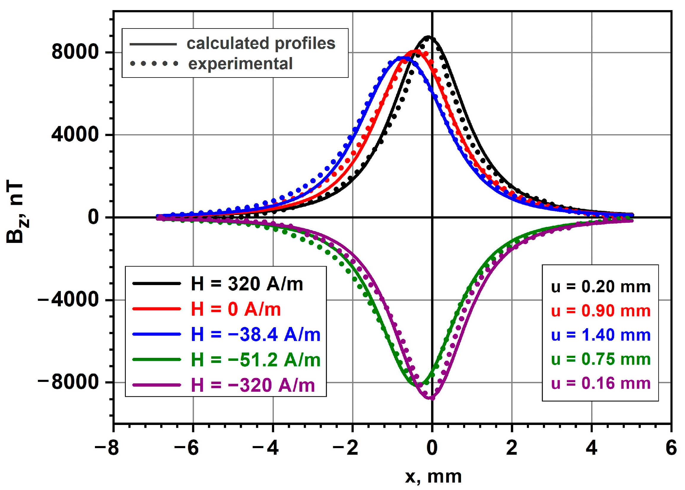
• Using the scanning GMI magnetometry technique, measurements of weak local magnetic fields were made near the segments of Fe-rich microwires being magnetized by external longitudinal fields. Characteristic values were determined for the switching magnetic field, the average magnetization of the microwire and the closure domain width for different values of the magnetizing fields.
• A calculation method is proposed that allows for the determination, based on the measured magnetic fields, of the magnitude and distribution of magnetization along a microwire segment.
• It was determined that the data obtained via the scanning GMI magnetometry technique are consistent with the findings received by vibrating sample magnetometry.

References

1. Phan, M.H.; Peng, H.X. Giant magnetoimpedance materials: Fundamentals and applications. Prog. Mater. Sci. 2008, 53, 323–420. [Google Scholar] [CrossRef]
2. Varga, R. Fast domain wall dynamics in thin magnetic wires. In Magnetic Properties of Solids; Tamayo, K.B., Ed.; Nova Science Publishers, Inc.: New York, NY, USA, 2009; Chapter 6; pp. 251–272. [Google Scholar]
3. Elmanov, G.N.; Kozlov, I.V.; Dzhumaev, P.S.; Chernavskii, P.A.; Kostitsyna, E.V.; Tarasov, V.P.; Ignatov, A.S.; Gudoshnikov, S.A. Effect of heat treatment on phase transformations and magnetization of amorphous Co69Fe4Cr4Si12B11 microwires. J. Alloys Compd. 2018, 741, 648–655. [Google Scholar] [CrossRef]
4. Kostitsyna, E.V.; Gudoshnikov, S.A.; Popova, A.V.; Petrzhik, M.I.; Tarasov, V.P.; Usov, N.A.; Ignatov, A.S. Mechanical properties and internal quenching stresses in co-rich amorphous ferromagnetic microwires. J. Alloys Compd. 2017, 707, 199–204. [Google Scholar] [CrossRef]
5. Popova, A.V.; Odintsov, V.I.; Menshov, S.A.; Kostitsyna, E.V.; Tarasov, V.P.; Zhukova, V.; Zhukov, A.; Gudoshnikov, S.A. Continuous control of a resistance in Co-rich amorphous ferromagnetic microwires during DC Joule heating. Intermetallics 2018, 99, 39–43. [Google Scholar] [CrossRef]
6. Knobel, M.; Vázquez, M.; Kraus, L. Giant magnetoimpedance. Handb. Magn. Mater. 2003, 15, 497–563. [Google Scholar] [CrossRef]
7. Zhukov, A.; Ipatov, M.; Zhukova, V. Advances in Giant Magnetoimpedance of Materials. Handb. Magn. Mater. 2015, 24, 139–236. [Google Scholar] [CrossRef]
8. Ipatov, M.; Zhukova, V.; Zhukov, A.; Gonzalez, J. Magnetoimpedance sensitive to dc bias current in amorphous microwires. Appl. Phys. Lett. 2010, 97, 252507. [Google Scholar] [CrossRef]
9. Gudoshnikov, S.A.; Tarasov, V.P.; Odintsov, V.I.; Liubimov, B.Y.; Menshov, S.A.; Popova, A.V. Correlation of electrical and magnetic properties of co-rich amorphous ferromagnetic microwires after dc joule heating treatment. J. Alloys Compd. 2020, 845, 156220. [Google Scholar] [CrossRef]
10. Gudoshnikov, S.; Usov, N.; Nozdrin, A.; Ipatov, M.; Zhukov, A.; Zhukova, V. Highly sensitive magnetometer based on the off-diagonal GMI effect in Co-rich glass-coated microwire. Phys. Status Solidi 2014, 211, 980–985. [Google Scholar] [CrossRef]
11. Uchiyama, T.; Ma, J. Development of pico tesla resolution amorphous wire magneto-impedance sensor for bio-magnetic field measurements. J. Magn. Magn. Mater. 2020, 514, 167148. [Google Scholar] [CrossRef]
12. He, D.; Shiwa, M. A Magnetic Sensor with Amorphous Wire. Sensors 2014, 14, 10644–10649. [Google Scholar] [CrossRef] [PubMed]
13. Bardin, I.V.; Bautin, V.A.; Gudoshnikov, S.A.; Seferyan, A.G.; Usov, N.A.; Ljubimov, B.Y. Investigation of quasi-stationary magnetic fields of corrosion currents of zinc-copper cells using giant magneto-impedance magnetometer. Corros. Sci. 2016, 109, 257–262. [Google Scholar] [CrossRef]
14. Gudoshnikov, S.; Tarasov, V.; Liubimov, B.; Odintsov, V.; Venediktov, S.; Nozdrin, A. Scanning magnetic microscope based on magnetoimpedance sensor for measuring of local magnetic fields. J. Magn. Magn. Mater. 2020, 510, 166938. [Google Scholar] [CrossRef]
15. Gudoshnikov, S.; Danilov, G.; Gorelikov, E.; Grebenshchikov, Y.; Odintsov, V.; Venediktov, S. Scanning magnetometer based on magnetoimpedance sensor for measuring a remnant magnetization of printed toners. Measurement 2022, 204, 112045. [Google Scholar] [CrossRef]
16. Varga, R.; Garcia, K.L.; Vázquez, M.; Vojtanik, P. Single-Domain Wall Propagation and Damping Mechanism during Magnetic Switching of Bistable Amorphous Microwires. Phys. Rev. Lett. 2005, 94, 017201. [Google Scholar] [CrossRef]
17. Zhukov, A. Domain wall propagation in a Fe-rich glass-coated amorphous microwire. Appl. Phys. Lett. 2001, 78, 3106–3108. [Google Scholar] [CrossRef]
18. Kabanov, Y.; Zhukov, A.; Zhukova, V.; Gonzalez, J. Magnetic domain structure of wires studied by using the magneto-optical indicator film method. Appl. Phys. Lett. 2005, 87, 142507. [Google Scholar] [CrossRef]
19. Zhukov, A.; Zhukova, V. Magnetic Properties and Applications of Ferromagnetic Microwires with Amorphous and Nanocrystalline Structure; Nanotechnology Science and Technology Series; Nova Science Publishers: New York, NY, USA, 2009; Available online: https://books.google.ru/books?id=EqRuPgAACAAJ (accessed on 5 April 2023).
20. Vazquez, M. Magnetic Nano- and Microwires: Design, Synthesis, Properties and Applications; Woodhead Publishing Series in Electronic and Optical Materials; Elsevier Science: Amsterdam, The Netherlands, 2015; Available online: https://books.google.ru/books?id=xMmcBAAAQBAJ (accessed on 5 April 2023).
21. Allwood, D.A.; Xiong, G.; Faulkner, C.C.; Atkinson, D.; Petit, D.; Cowburn, R.P. Magnetic domain-wall logic. Science 2005, 309, 1688–1692. [Google Scholar] [CrossRef] [PubMed]
22. Parkin, S.; Yang, S.-H. Memory on the racetrack. Nat. Nanotech. 2015, 10, 195–198. [Google Scholar] [CrossRef] [PubMed]
23. Lei, N.; Devolder, T.; Agnus, G.; Aubert, P.; Daniel, L.; Kim, J.-V.; Zhao, W.; Trypiniotis, T.; Cowburn, R.P.; Chappert, C.; et al. Strain-controlled magnetic domain wall propagation in hybrid piezoelectric/ferromagnetic structures. Nat. Commun. 2013, 4, 1378. [Google Scholar] [CrossRef] [PubMed]
24. Gudoshnikov, S.; Usov, N.; Zhukov, A.; Zhukova, V.; Palvanov, P.; Ljubimov, B.; Serebryakova, O.; Gorbunov, S. Evaluation of use of magnetically bistable microwires for magnetic labels. Phys. Status Solidi A 2011, 208, 526–529. [Google Scholar] [CrossRef]
25. Moriya, R.; Hayashi, M.; Thomas, L.; Rettner, C.; Parkin, S.S.P. Dependence of field driven domain wall velocity on cross-sectional area in Ni65Fe20Co15 nanowires. Appl. Phys. Lett. 2010, 97, 142506. [Google Scholar] [CrossRef]
26. Richter, K.; Varga, R.; Kováč, J.; Zhukov, A. Controlling the Domain Wall Dynamics by Induced Anisotropies. IEEE Trans. Magn. 2012, 48, 1266–1268. [Google Scholar] [CrossRef]
27. Zhukova, V.; Corte-Leon, P.; González-Legarreta, L.; Talaat, A.; Blanco, J.M.; Ipatov, M.; Olivera, J.; Zhukov, A. Review of Domain Wall Dynamics Engineering in Magnetic Microwires. Nanomaterials 2020, 10, 2407. [Google Scholar] [CrossRef] [PubMed]
28. Zhukov, A.; Blanco, J.M.; Ipatov, M.; Zhukova, V. Fast magnetization switching in thin wires: Magnetoelastic and defects contributions. IEEE Sens. Lett. 2013, 11, 170–176. [Google Scholar] [CrossRef]
29. Huang, S.-H.; Lai, C.H. Domain-wall depinning by controlling its configuration at notch. Appl. Phys. Lett. 2009, 95, 032505. [Google Scholar] [CrossRef]
30. Calle, E.; Vazquez, M.; del Real, R.P. Time-resolved motion of a single domain wall controlled by a local tunable barrier. J. Magn. Magn. Mater. 2020, 498, 166093. [Google Scholar] [CrossRef]
31. Vereshchagin, M.; Baraban, I.; Leble, S.; Rodionova, V. Structure of head-to-head domain wall in cylindrical amorphous ferromagnetic microwire and a method of anisotropy coefficient estimation. J. Magn. Magn. Mater. 2020, 504, 166646. [Google Scholar] [CrossRef]
32. Antonov, A.S.; Borisov, V.T.; Borisov, O.V.; Pozdnyakov, V.A.; Prokoshin, A.F.; Usov, N.A. Residual quenching stresses in amorphous ferromagnetic wires produced by an in-rotating-water spinning process. J. Phys. D Appl. Phys. 1999, 32, 1788. [Google Scholar] [CrossRef]
33. Vázquez, M.; Zhukov, A.P. Magnetic properties of glass-coated amorphous and nanocrystalline microwires. J. Magn. Magn. Mater. 1996, 160, 223–228. [Google Scholar] [CrossRef]
34. Aragoneses, P.; Blanco, J.M.; Dominguez, L.; Gonzalez, J.; Zhukov, A.; Vazquez, M. The stress dependence of the switching field in glass-coated amorphous microwires. J. Phys. D Appl. Phys. 1998, 31, 3040. [Google Scholar] [CrossRef]
35. Varga, R. Magnetization processes in glass-coated microwires with positive magnetostriction. Acta Phys. Slovaca 2012, 62, 411–518. [Google Scholar] [CrossRef]
36. Gudoshnikov, S.A.; Grebenshchikov, Y.B.; Ljubimov, B.Y.; Palvanov, P.S.; Usov, N.A.; Ipatov, M.; Zhukov, A.; Gonzalez, J. Ground state magnetization distribution and characteristic width of head to head domain wall in Fe-rich amorphous microwire. Phys. Status Solidi A 2009, 206, 613–617. [Google Scholar] [CrossRef]
37. Zhukova, V.; Zhukov, A.; Blanco, J.M.; Gonzalez, J.; Ponomarev, B.K. Switching field fluctuations in a glass coated Fe-rich amorphous microwire. J. Magn. Magn. Mater. 2002, 249, 131–135. [Google Scholar] [CrossRef]
38. Zhukova, V.; Blanco, J.M.; Rodionova, V.; Ipatov, M.; Zhukov, A. Domain wall propagation in micrometric wires: Limits of single domain wall regime. J. Appl. Phys. 2012, 111, 07E311. [Google Scholar] [CrossRef]
39. Gudoshnikov, S.; Usov, N.; Zhukov, A.; Gonzalez, J.; Palvanov, P. Measurements of stray magnetic fields of amorphous microwires using scanning microscope based on superconducting quantum interference device. J. Magn. Magn. Mater. 2007, 316, 188–191. [Google Scholar] [CrossRef]
40. Gudoshnikov, S.A.; Venediktov, S.N.; Gorbunov, S.A.; Kozlov, A.N.; Prokhorova, Y.V.; Serebryakova, O.N.; Sitnov, Y.S.; Skomarovskii, V.S. An automated compact vibromagnetometer for investigating soft magnetic materials. Meas. Tech. 2010, 53, 88–92. [Google Scholar] [CrossRef]
41. Hernando, B.; Sánchez, M.L.; Prida, V.M.; Santos, J.D.; Olivera, J.; Belzunce, F.J.; Badini, G.; Vázquez, M. Magnetic domain structure of amorphous Fe73.5Si13.5B9Nb3Cu1 wires under torsional stress. J. Appl. Phys. 2008, 103, 07E716. [Google Scholar] [CrossRef]
Figure 1. Schematic representation of scanning GMI magnetometer. The inset shows the orientation of the studied microwire, GMI sensor, and magnetic field generated by means of HCs.
Metals 13 00800 g001
Figure 2. Magnetic images of 6.5-mm microwire sample, at a distance of 1 mm, in longitudinal magnetic field of 400 A/m. (a) Two-dimensional magnetic image of microwire, (b) magnetic profile of Bz(x) along axis “1” parallel to the microwire centerline. The left and right insets show transverse profiles of Bz(y), measured along axes “2” and “3”, respectively.
Metals 13 00800 g002
Figure 3. Magnetic images of 6.5-mm microwire obtained with different external longitudinal magnetic fields.
Metals 13 00800 g003
Figure 4. Magnetic images of a 15.5 mm microwire sample, at a height of 1 mm, in longitudinal magnetic field of 400 A/m. (a) Two-dimensional magnetic image of the microwire; (b) magnetic profile of the induction component of Bz(x) along the microwire centerline. The inset shows the expected distribution of magnetization in the closure domain of the microwire.
Metals 13 00800 g004
Figure 5. Experimental and theoretical profiles of magnetic induction component Bz(x) above the right-hand end of a 15.5 mm microwire in external longitudinal field Hx of different magnitudes. On the left are values of external longitudinal magnetic fields relevant to the presented curves; on the right are calculated values of the width u of uniform distribution of magnetic charges at the end of the microwire.
Metals 13 00800 g005
Figure 6. Hysteresis curve of a 6.5-mm microwire. Insets 1–4 show profiles of Bz(x), along the microwire centerline at a height of 1 mm with different values of magnetic field (points 1–4 on the hysteresis loop), measured by means of a scanning GMI magnetometer.
Metals 13 00800 g006
Disclaimer/Publisher’s Note: The statements, opinions and data contained in all publications are solely those of the individual author(s) and contributor(s) and not of MDPI and/or the editor(s). MDPI and/or the editor(s) disclaim responsibility for any injury to people or property resulting from any ideas, methods, instructions or products referred to in the content.