Article

Prediction of Recrystallization Structure of 2A12 Aluminum Alloy Pipe Extrusion Process Based on BP Neural Network

1
Key Laboratory for Advanced Materials Processing Technology, Ministry of Education of China, Beijing 100084, China
2
Department of Mechanical Engineering, Tsinghua University, Beijing 100084, China
*
Author to whom correspondence should be addressed.
Metals 2023, 13(4), 664; https://doi.org/10.3390/met13040664
Submission received: 28 February 2023 / Revised: 25 March 2023 / Accepted: 26 March 2023 / Published: 27 March 2023

Abstract

:
2A12 aluminum alloy is a high-strength aerospace alloy. During its extrusion process, the extrusion process parameters have a great impact on the microstructure evolution of the extruded products. There are three extrusion process parameters controlled in the actual project, which are the initial temperature of billet, the initial temperature of die and the extrusion speed. Combined with a back propagation (BP) neural network and finite element method (FEM) simulation, based on the constitutive equation and recrystallization evolution process of 2A12 aluminum alloy, this paper establishes a prediction model for the grain size of extruded pipe by these three extrusion process parameters. This paper used a 35MN extruding machine for a production verification of 2A12 pipe. The results show that the predicted grain size is 3% smaller than the actual size.

1. Introduction

2A12 aluminum alloy belongs to the Al–Cu–Mg-series alloy, which is widely used in aerospace, radar, automobile and other industrial sectors for its perfect properties such as high strength, good formability and machinability [1]. Its chemical composition is similar to 2024 aluminum alloy in American standard [2,3]. Its performance is mainly determined by melting and casting process, extrusion process and heat treatment process [4]. The metal strength decreases, and the metal fluidity improves as the temperature increases. Therefore, hot forming technology is often used in material forming [5]. The pipe production processes mainly include rolling, hot extrusion, drawing, forging and other methods [6]. During hot extrusion, grain refinement, strain strengthening, solid solution strengthening and precipitation hardening increase the strength of the formed tube [7,8,9].
It is critical in extrusion process to control the maximum extrusion force and the exit temperature of the extrusion die. The properties of the formed pipe are related to the microstructure of the formed material, while the die exit temperature distribution has a significant influence on the microstructure, mechanical properties, and surface quality of the extruded products [10]. The temperature of the formed pipe at the die exit is influenced by the combination of environmental heat dissipation, material-forming heat and frictional heat during the flow of the billet (including friction between the billet and the friction between the billet and the die). It is related to the process parameters such as friction coefficient, the extrusion material, the initial billet temperature, the die temperature, the extrusion speed and so on.
Artificial neural networks, as a hot topic of research in the field of artificial intelligence, utilize information processing techniques to simulate human brain neurons and construct various models by forming different networks according to different connection methods. As a typical multilayer forward artificial neural network, BP neural networks are widely utilized in pattern recognition, function approximation, classification and data compression. With the advancement of machine learning, intelligent algorithms have been introduced as an effective method to solve nonlinear problems, which are extensively used in the field of engineering computation for applications such as material rebound calculation [11], analysis of the influence of chemical composition of metal materials on material properties [12,13], material constitutive modeling [14,15], maximum extrusion force calculation in the extrusion process [16,17], optimization of extrusion process parameters, analysis of the influence of chemical composition of metal materials on stress-strain curves [18] and other areas of processing.
To better describe the evolution of grain size during the extrusion process, this paper uses BP neural network to analyze the extrusion speed, billet temperature, die temperature and other process parameters through FEM simulation, and combine the constitutive model and recrystallization model of 2A12 aluminum alloy material to predict the grain size of each part of the extruded tube and obtain a complete grain size prediction model.
To accurately depict the evolution of microstructure material grain size during the extrusion process, this paper employs a BP neural network to analyze various process parameters, including extrusion speed, billet temperature, die temperature and other process parameters via FEM simulation. By integrating the constitutive model and recrystallization model of 2A12 aluminum alloy material, this approach predicts the grain size of every part of the extruded tube, resulting in a comprehensive grain size prediction model.

2. Constitutive Equation and Recrystallization Process Analysis of 2A12 Aluminum Alloy

2.1. Material Constitutive Model

To construct the 2A12 aluminum alloy material constitutive model, we conducted isothermal compression experiments on 2A12 samples using a Gleeble-1500D thermal compressor (Dynamic Systems Inc., Austin, TX, USA). The hot compressed samples were sized at ф 6 mm × 8 mm, heated from room temperature to the specified temperature at a heating rate of 10 °C/s, and held for 3 min to ensure the overall temperature of the extruded samples was uniform. Subsequently, the compressor compressed the specimen to 50% of the strain at the designed deformation rate, and a T-type thermocouple was welded onto the surface of the samples to measure its temperature. Table 1 shows the composition of the 2A12 aluminum alloy examined in this study.
We conducted the experiments in four different billet temperatures ranging from 360 °C to 480 °C, with each temperature being 40 °C apart. We use four strain rates, which are 0.01  s 1 , 0.1  s 1 , 1  s 1 , and 10  s 1 , respectively. In total, we performed 16 experiments, and Table 2 shows the parameters of the 16 thermal compression experiments. Figure 1 shows the 16 real stress–strain curves of the 2A12 aluminum alloy material obtained in the hot compression experiments.
The Arrhenius equation is the most widely used equation for describing the correlation between flow stress, temperature, and strain rate, particularly at high temperatures. We can use the Zener–Hollomon parameter with an exponential equation to express the influence of temperature and strain rate on deformation behavior. The hyperbolic law utilized in the Arrhenius equation provides a more accurate approximation of the relationship between the Zener–Hollomon parameter and flow stress [14,15,19].
ε ˙ = A F σ exp Q R T
Z = ε ˙ exp Q R T
F σ = σ n α σ < 0.8 exp β σ α σ > 1.2 sinh α σ n f o r   a l l   σ
where  Z  is the Zener–Hollomon parameter,  ε ˙    is the strain rate ( s 1 );  σ  is the stress (MPa);  T  is the deformation temperature (K);  R  is the gas constant with a value of 8.314  J mol ×   K Q  is the heat deformation activation energy ( kJ mol );  F σ  is the stress function;  A α β n  and  n  are material constants.
Combining Equations (1)–(3) yields
l n Z = l n A + n l n s i n h α σ
Therefore, by drawing a figure of  l n A  and  l n s i n h α σ , and performing a linear fit of  l n A  and  l n s i n h α σ  we deduce that parameter  A = 3.076 × 10 16 .
According to Equations (1) and (3), we get
l n ε ˙ = l n A + n l n σ Q R T
n ε ˙ = l n A + β σ Q R T     β = α n
l n ε ˙ = l n A + n l n s i n h α σ Q R T
Equations (5)–(7) show that, when the temperature is invariant,  l n ε ˙  and  l n σ  are linear relations with slope  n l n ε ˙  and  σ  are linear relations with slope  β , which is  α n ; when the strain rate is invariant,  l n s i n h α σ  and  1 T  are linear relationships with a slope of  Q R .
According to the former discussion, making scatter plots of  l n ε ˙  and  l n σ l n ε ˙  and  σ l n s i n h α σ  and  1000 T  as shown in Figure 2 and performing a linear fit, we get  n = 6.738 α = 0.01313 Q = 228.668   kJ mol .
The final constitutive equation for the Arrhenius type of 2A12 aluminum alloy is given as Equation (8).
ε ˙ = × 10 16 × s i n h 0.01313 σ 6.738 exp 228668 / 8.31 T

2.2. Material Recrystallization Modeling

Extrusion of 2A12 aluminum alloy tubes is a problem of large plastic deformation under high-temperature conditions. In previous studies, scholars have found that 2A12 plastic deformation at high temperatures produces dynamic recrystallization [20]. When the deformation strain is bigger than 2, we can nearly obtain complete material recrystallization microstructure [21]. Therefore, in the extrusion process of 2A12 aluminum alloy pipes, when we select a large extrusion ratio deformation, we can take the material microstructure as totally recrystallized microstructure, and the calculation of recrystallized grain size can be determined by Equation (9) [22].
D d r x = A 1 Z n 1
In Equation (9)  D d r x  is the dynamic recrystallization grain size,  A 1  and  n 1  are constants, and  Z  is the Zener–Hollomon parameter, which has been discussed in Section 2.1 and whose values are expressed as Equation (10).
Z = ε ˙ exp 228668 / 8.31 T
In Equation (10),  ε ˙  is the strain rate and  T  is the deformation temperature (K). Combining Equations (9) and (10), we obtain
D d r x = A 1 ε ˙ exp 228668 / 8.31 T n 1
From Equation (11) we can find that the recrystallized grain size is related to the strain rate and deformation temperature. To predict the grain size of the microstructure of 2A12 tubes during extrusion, we should calculate the values of the constant parameters  A 1  and  n 1  in Equation (11), so we should use the recrystallization microstructure of the 2A12 alloy after plastic deformation to calculate the constant values. In the study of the material constitutive structure relationship, 16 groups of 2A12 aluminum alloy materials have undergone hot extrusion deformation, and Figure 3a shows the samples of 2A12 materials after hot extrusion deformation.
The 16 extruded samples obtained after the Gleeble hot compression experiment were cut longitudinally, etched and polished to make metallographic observation samples. Figure 3b shows the completed metallographic observation samples after compression experiment. We used an electron microscope to observe the 16 samples, and Figure 4 and Figure 5 show the observed metallographic images. Figure 4 shows the initial microstructure before Gleeble compression.
Among the metallographic observation of the Gleeble specimens, Figure 5a shows that, with the compression of the Gleeble specimens, the dynamic recrystallized (DRX) grains of 2A12 aluminum alloy appear at the grain boundaries which are highlighted with a red circle. In the hot compression test, the dynamic recrystallization behavior of 2A12 aluminum alloy occurs, but because the strain is too small, which is only 0.5, the recrystallization behavior can only occur at the grain boundaries where the energy of the original grains is unstable.
We can see that the DRX grains are smaller than the original grains, and the DRX grains are not continuous, so we use the software named Image-Pro to measure the diameter of DRX grains. The grain diameter measurement is based on the principle of classifying the entire image by pixel level, dividing the length of measuring scale by the pixels in the image, and then measuring the number of pixels in the direction of dynamic recrystallization grain diameter, and multiplying them together to obtain the diameter of dynamic recrystallization grain. Among Figure 4, Figure 5 and Figure 6, each pixel represents about 0.027 μm, so we use two decimal places to express the grain size. According to this method, we measure the initial grain size before Gleeble compression to be 25.32 μm.
We measure the grain diameters of 100 dynamic recrystallized grains in the sample metallographic Figure 5 and Figure 6 and take the average value as the dynamic recrystallized grain diameter at that temperature and strain rate condition. After the measurements, Table 3 shows the dynamic recrystallized grain diameter and its root mean squared error (RMSE) of each specimen.
Previous studies have shown that the recrystallized grain size of metals increases with increasing deformation temperature and decreasing strain rate [23]. By looking at the table of recrystallized grain size of 2A12 aluminum alloy, we can see that the recrystallized grain size of 2A12 aluminum alloy also increases with increasing deformation temperature and decreasing strain rate.
Taking the logarithm of both sides of Equation (9), we can obtain
l n D d r x = l n A 1 n 1 l n Z
From Equation (12), we can see that  ln D d r x  and  l n Z  are a first-order linear relationship with a slope of  n 1  and an intercept of  l n A 1 .
The deformation temperature and strain rate in Table 3 are brought into Equation (10) to find out  l n Z , and we take the recrystallized grain size in Table 3 and the Zener–Hollomon parameter logarithmically to make the relationship of  l n D d r x l n Z  as shown in Figure 7.
The recrystallized grain size of 2A12 aluminum alloy can be calculated as Equation (13) by bringing the fitted values into Equation (9) after a linear fit to Figure 7.
D d r x = 81.3711 × Z 0.05783
According to Equation (13) we can obtain the calculated grain size as Table 4:
From Table 4 we can see that the biggest relative error is 12.16 %, and the most errors are lower than 10 %, while the RSME is 0.58, so we can assume that the Equation (13) meets the accuracy requirements of 2A12 alloy.
In Equation (13) we can see that the recrystallized grain size is mainly related to the Zener-Holloman parameter, while in Equation (10) we can see that the Zener–Hollomon parameter is determined by the strain rate and the recrystallization temperature, as the strain rate is determined by the extrusion speed and extrusion ratio. The strain rate can be calculated in Equation (14) [24]
ε ˙ = l n λ · V j A t A z 0.4 D 2 2 0.75 D 1 2 3 2 0.5 D 2 3 0.75 D 1 3
In Equation (14),  ε ˙  is the strain rate.  λ  is the extrusion ratio, whose value is 7.81 in this paper.  V j  is the extrusion speed.  A t  is the inner ring area of the extrusion die, whose value is 7854  mm 2 A z  is the area of the mandrel, which is 5674  mm 2 D 2  is the outer diameter of billet, which is 170 mm.  D 1  is the outer diameter of the pipe, whose value is 100 mm. Therefore, in the actual tube extrusion process, when the extrusion speed and extrusion ratio are determined, the recrystallization grain size is only related to the extrusion exit temperature. Therefore, the following FEM model is needed to predict the extrusion exit temperature of the pipe extrusion process.

3. FEM Analysis of Extrusion Process

In the actual production process, once the product is determined, the extrusion die is also determined. In that condition, the adjustable parameters during the production process are mainly the initial heating temperature of the billet, the die temperature, and the extrusion speed. 
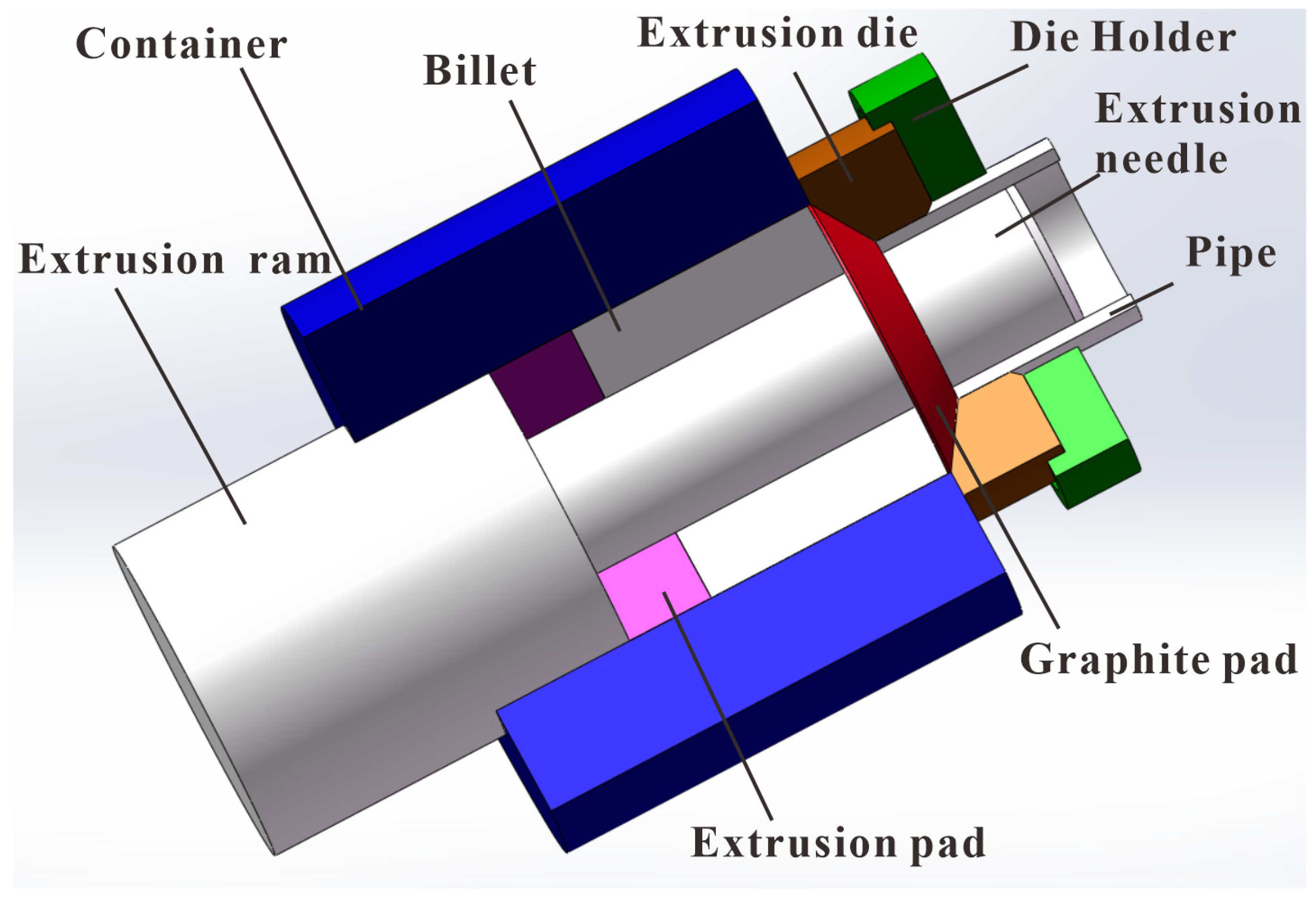
Figure 8 shows a three-dimensional diagram of the pipe extrusion process. In this paper, the production parameters in FEM simulation set as following: the initial heating temperature of the billet is 300 °C, 350 °C, 400 °C and 450 °C, the initial heating temperature of the die is 20 °C, 100 °C, 200 °C and 300 °C, and the extrusion speed is 0.5 mm/s, 1 mm/s, 2 mm/s and 5 mm/s. A total of 4 × 4 × 4 = 64 sets of simulations are conducted.
From the discussion in Section 2.2, to build a model to predict the microstructure of 2A12 tube extrusion process, we should predict the extrusion exit temperature of the tube first. Deform, as a finite element analysis software, is used widely in extrusion nowadays [25]. Moreover, because tube extrusion is a strictly axisymmetric model, to simplify the extrusion model and improve simulation speed, this paper builds a Deform-2D model for 2A12 pipe extrusion. In the simulation calculations, we use the skyline method and Newton’s iteration method to calculate the simulation result and import the constitutive model of 2A12 aluminum alloy obtained in Section 2.1 into the Deform software material library. Table 5 shows other Deform Analog Input Parameters [26].
Considering the actual tube production process, the simulation is set as following three stages: billet transportation, machine preparation, and extrusion.
In tube extrusion process, we should first transport the billet from the heating furnace to the extrusion location. 
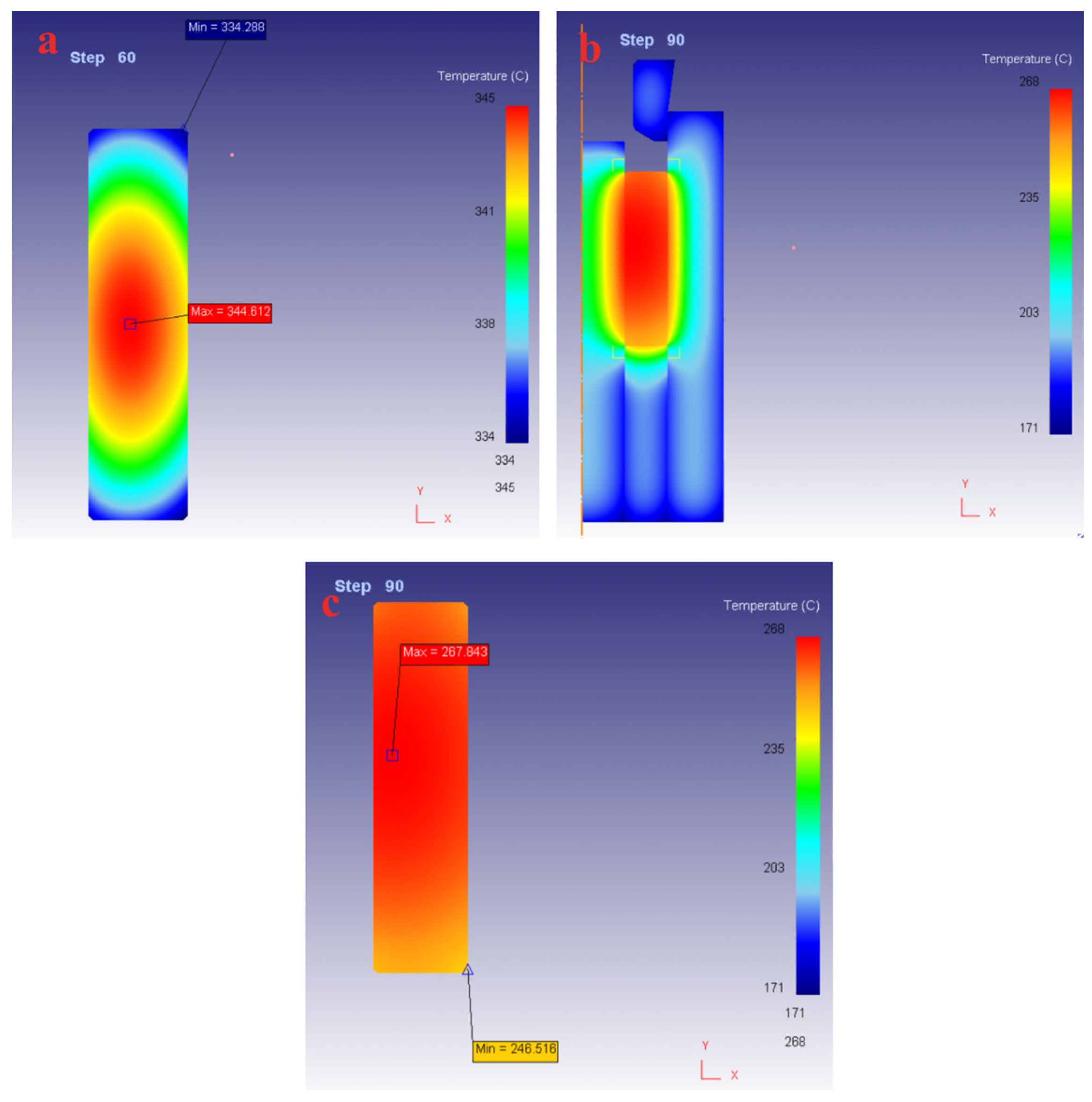
Figure 9a shows the temperature distribution of a billet of 2A12 aluminum alloy heated to 400 °C after 60 s of air-cooling, with an internal diameter of 85 mm, an external diameter of 170 mm, and a height of 170 mm. We can see that the core of the billet has the highest temperature and the rounded corner near the outside has the lowest temperature, but the overall temperature difference is small.
After placing the billet on the extrusion needle, the operator starts the extrusion machine and lets the machine reach the extrusion position quickly. In this condition, the billet is in contact with the extrusion mandrel, extrusion barrel and extrusion pad, and this process is the interface heat transfer. The simulation of Figure 8b,c sets the temperature of the extrusion mandrel, extrusion barrel, extrusion pad and extrusion die at 200 °C. The expected time for this process is 30 s. Figure 9b shows the overall temperature after 30 s interface heat transfer. Figure 9c shows the billet temperature after 30 s interface heat transfer. We can find that the heat dissipation between the billet and the die makes the heat loss of the billet more than the heat loss during air cooling, and the lowest temperature of the billet is the outer ring of the lower right corner in contact with the sleeve and the lower extrusion pad, but the temperature difference inside the billet is still small.
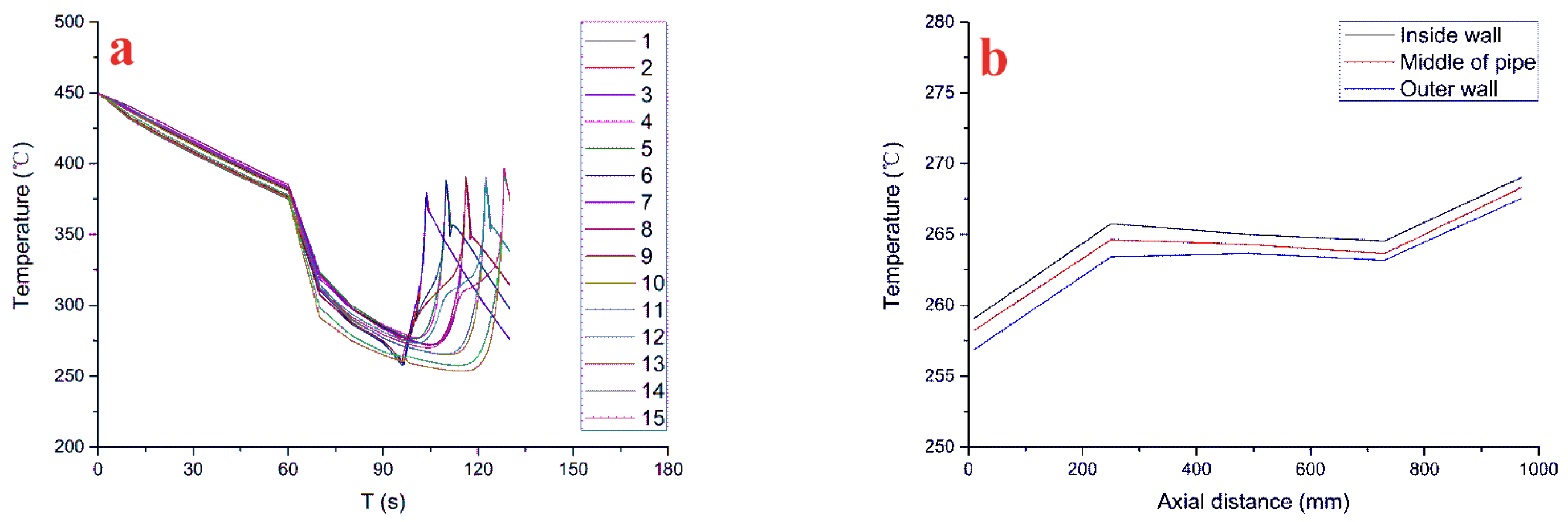
During the extrusion process, the focus is on the billet temperature at the extrusion exit of the die, as this is where the plastic deformation is most intense and where the temperature is highest during the extrusion deformation, which determines the grain size and mechanical properties of the formed pipe. Since the previously discussed extruded finished pipe has an inner diameter of 85 mm, an outer diameter of 100 mm, and a length of about 1 m, the points are taken along the extrusion direction and the vertical extrusion direction respectively in the simulation model of the extrusion process. Along the diameter direction, we take three points at the diameters of 85 mm, 92.5 mm, and 100 mm of the finished pipe; along the extrusion direction, we take five points at the extrusion lengths of 10 mm, 250 mm, 490 mm, 730 mm and 970 mm. In total, we select 3 × 5 = 15 points, and the points are named as follows: when the coordinates are d = 85 mm and l = 10 mm, it is the first point. When d = 92.5 mm, l = 10 mm is the second point, and so on. Set these 15 points as material flow following, record the temperature change of the 15 points during the extrusion process, and extract the extrusion exit temperature for further analysis.
In Figure 10a, we can see that the billet temperature drops rapidly during the air-cooling and contact heat-dissipation process. When the extrusion process begins, there is a large temperature rise, which means the material at this point passes through the extrusion exit, where the temperature is highest. After the extrusion passes this point, the material becomes extruded in the tube state and is in the air-cooled state and the temperature drops. In this figure, we can see that the radial temperature changes in the extrusion exit temperature difference are not large.
In Figure 10b we can see that the temperature at the inner point is the highest, and the temperature at the outer point is the lowest during extrusion. Because the wall thickness of the extruded pipe is too small, only 7.5 mm, and the extrusion exit temperature in the radial direction are very close, the maximum temperature difference is 5 °C, so the temperature distribution of the breakthrough extrusion temperature along the radial direction can considered uniform, only to think about the temperature distribution in the axial direction. Therefore, we take the radial extrusion exit temperature which is obtained in the FEM simulation average value as the axial location temperature, so we obtain five new temperature points to characterize the microstructure of pipe extrusion. The axial coordinate of 10 mm point is set as 1 point, and in turn axial distance of 970 mm point is set as five points.
In summary, the FEM simulation obtains 64 sets of extrusion exit temperature results which including five different extrusion exit-temperature outputs and three different process parameters. BP neural network in Section 4 will use these data for training and predicting.

4. BP Neural Network Prediction Model

BP neural network (back propagation neural network) can fit nonlinear models well and is now widely used in engineering model prediction. Its main features are the signal forward propagation and the error backward propagation. In the signal-propagation process, the input signal is weighted and inputted to the hidden layer, and after solving in the hidden layer, it is weighted again and input to the output layer, and the expected value is obtained after solving in the output layer. When there is an error in the output layer that does not achieve the desired output, the error is back-propagated and the network weights and bias between the layers are adjusted so that the predicted output changes until the error approaches the expectations.
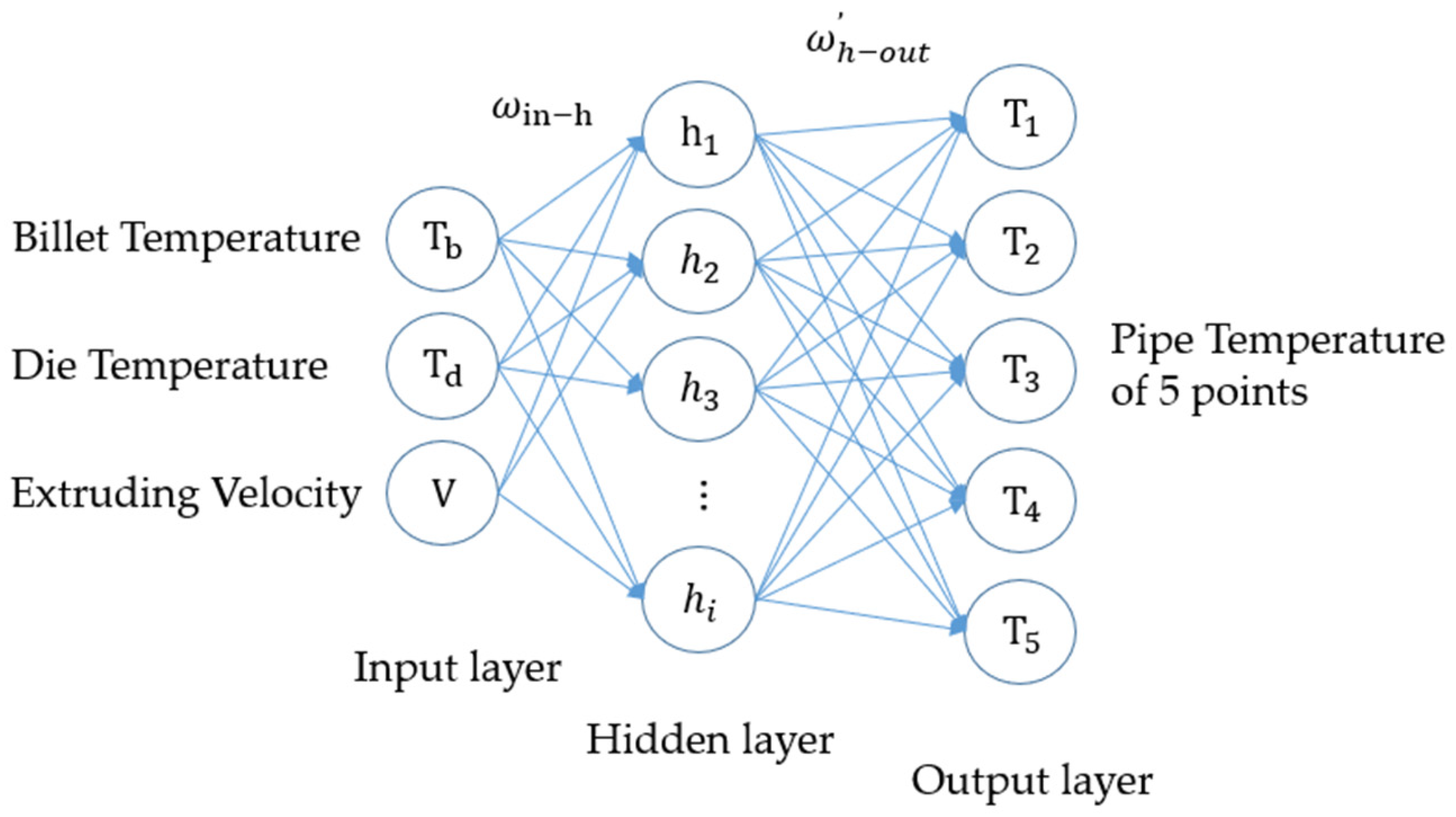
Figure 11 shows the structure of the BP neural network with three input units, five output units and one hidden layer. In a complete neural network, there are an input layer, several hidden layers, and an output layer, where the hidden layer numbers can change according to the data processing requirements, and we can set multiple hidden units in each hidden layer. The neurons in each layer are interconnected, and the neurons within the same layer are not connected. The data in the input layer are normalized first. After weighting, it is assigned to the hidden layer, which calculates the input values by the excitation function σ(x) and passes the calculation results to the output layer after second weighting. When there is an error between the predicted output and the desired output, the error is propagated backward, and the weights from the hidden layer to the output layer are adjusted first, and then the weights from the input layer to the hidden layer are adjusted. The above steps will not stop until the prediction model meets the accuracy requirements.
Considering the computation time and efficiency, this paper chooses to use a BP neural network with one hidden layer, and combines the empirical formula of the BP neural network to determine the number of nodes in the hidden layer:
n 1 = 2 m + 1
or
n 1 = n + m + a
In Equations (15) and (16),  n 1  is the number of nodes in the hidden layer,  n  is the number of inputs,  m  is the number of outputs, and  a  is a constant, whose value is between 1 and 10.
In the prediction of this paper, the number of input nodes is 3, which is the initial temperature of the billet, the initial temperature of the die, and the extrusion speed, and the number of output nodes is 5, which is the extrusion exit temperature at five points. According to the above equation, the number of nodes in the hidden layer is 4–13. After testing in the actual training, we choose a three-layer neural network with one hidden layer and eight neurons for the corresponding calculation, and the neural network of this structure can achieve a better balance of computational accuracy and computational time. We use the BP neural network module in Matlab for prediction simulation. The activation function of the BP neural network takes the form of a sigmoid function. The sigmoid function is expressed as followed:
O u t i = f n e t j = 1 1 + e k n e t j
where  k  is a constant,  n e t j  is the weighted sum of the  j t h  neuron for input received from the preceding layer with  n  neurons, which can be expressed as followed:
n e t j = i = 1 n w i j x i
where  w i j  is the weight of the  j t h  neuron in the previous layer,  x i  is the output of the  i t h  neuron in the previous layer.
The detailed training parameters are listed as follows: the number of training times is 1000 times, the learning efficiency is 0.01, and the minimum error of the training target is 0.0000001.
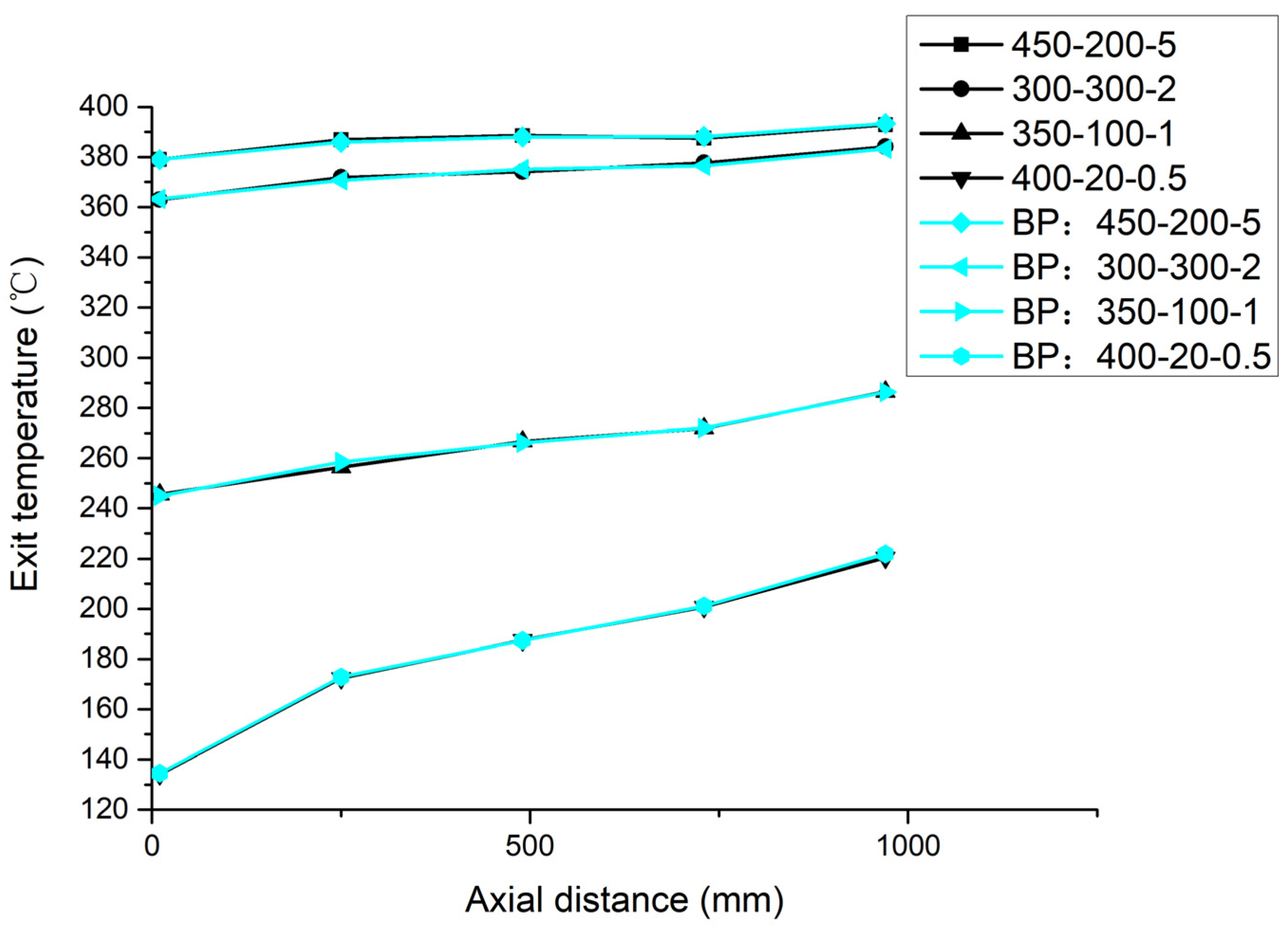
During the experiment, the 64 sets of parameters obtained from the Deform-2D simulation were divided into 60 training groups and 4 experimental groups. We select 450–200–5, 300–300–2, 350–100–1, and 400–20–0.5 for the 4 experimental groups (the order of experimental parameters were the initial temperature of the billet (°C), the initial temperature of the die (°C), and the extrusion speed (mm/s). There are four different initial temperatures of the billet, the initial temperature of the die, and extrusion speed respectively in the experimental set, which can have good generalizability.
After the 60 sets of training, we use the neural network to predict the remaining 4 experiment groups, and Table 6 and Figure 12 show the BP neural network predicted results and experimental results.
Figure 12 shows that the predicted temperature in blue line and the temperature obtained from the original simulation in black line almost overlap. After analyzing the data in Table 5, we can find that the BP neural network used in this paper can better fit the extrusion exit temperature during the pipe extrusion process.

5. Experimental Verification

The extrusion of 2A12 tube was performed at the Institute of Metal Research, Chinese Academy of Sciences, to verify the reliability of the models established in Section 2, Section 3 and Section 4. Figure 13a shows the 35MN multi-function extruding machine which is used in this paper. The billet and die shapes and sizes are same as the Deform simulation used in Section 3. We preheated the billet form room temperature to 450 °C in 1 h in a heating furnace and held for 3 h to achieve a uniform internal temperature of the billet, and preheated the die to 200 °C in the heating furnace and held for 3 h to achieve uniform internal temperature of the die, and set the extrusion speed at 5 mm/s. Then we began the extrusion process. Figure 13b shows the finished extrusion pipe.
In Figure 13b, ① is the initial extruded part and ② is the final extruded part. At ③, the distance to the initial extrusion position ① of the 2A12 pipe is about 10 mm. We took samples along the pipe extrusion direction and vertical to the pipe extrusion direction in spot ③ and examined these metallographic organization after corrosion and polishing. Figure 14 shows the samples’ metallographic images.
Figure 14a shows the grains along the extrusion direction are almost recrystallized grains after rapid large plastic deformation, and the grain size is relatively more uniform and smaller, and Figure 14b shows the grains along the vertical extrusion direction are significantly elongated.
Figure 15 shows that during the extrusion process, the effective strain of the grain is bigger than 2. When the deformation strain is bigger than 2, we can nearly obtain complete material recrystallization microstructure [21], so we can take the grains along the extrusion direction as complete dynamic recrystallization microstructure, while the grains along the vertical extrusion direction are significantly elongated equiaxed grains with no recrystallization properties.
We take the actual pipe production process parameters which including the 450 °C initial billet heating temperature, the 200 °C initial heating temperature of the die, the extrusion speed of 5 mm/s into the BP neural network prediction model of exit temperature established in the Section 2, Section 3, and Section 4. According to Equation (14), we can obtain that the strain rate of this tube extrusion is 0.028  s 1 . The BP neural network shows that the temperature of spot ③ in Figure 13b is 379.0 °C. Bringing this temperature into the prediction formula if the recrystallization grain size of 2A12 aluminum alloy, we find that the recrystallization grain size in spot ③ is 8.73 μm. The grain size is 9.01 μm which is measured in the metallographic image. The relative error is 3.11%, which is very small, so we believe the prediction model is reliable. The prediction size is smaller than the production size. One of the reasons is that in the extrusion process, although there is a large plastic deformation, there are still some metal tissues that cannot completely undergo a recrystallization transformation. The recrystallized tissues at this time occupy the majority, but there are still a small number of untransformed tissues which will make the overall grain size of the material larger.
In summary, the predicted model established in this paper is generally reliable. In engineering, we can predict the grain size of the extrusion material by a BP neural network.

6. Conclusions

In this paper, we establish a prediction model based on BP neural network and material constitutive model to predict the microscopic grain size of 2A12 aluminum alloy tube extrusion. Through the establishment of the material constitutive equation of 2A12 aluminum alloy, the observation of Gleeble samples, the simulation of the extrusion process and the training of the BP neural network, and the verification of the actual extrusion experiment, the prediction deviation of the established model for the micro-grain size of 2A12 aluminum alloy tube extrusion is finally 3%. Therefore, the prediction model in this paper can be used in engineering to predict the microstructure evolution of 2A12 aluminum alloy pipe extrusion.
For pipe extrusion with small wall thickness, we can regard the exit temperature to be constant in the radial direction, and the metallographic organization of the metal will be the same, and we should only study the axial temperature differences. However, the extrusion of thick-walled pipes will have more significant differences. In the study of thick-walled pipes one should not only consider its axial differences but also pay attention to its radial exit temperature and metallographic organization differences.
In the extrusion process, although the material has a large plastic deformation, there is still some metal tissue that cannot completely undergo recrystallization transformation. The recrystallized tissue at this time occupies the majority, but there are still a small number of incomplete broken tissues, and transformation of the organization will make the overall grain size of the material larger. To predict the metallographic organization and pipe properties of pipe extrusion more accurately, a detailed study of this problem is needed subsequently.

Supplementary Materials

The following supporting information can be downloaded at: https://www.mdpi.com/article/10.3390/met13040664/s1, FEM data.

Author Contributions

H.J. performed the experiment and wrote the paper; R.W. analyzed and discussed the results and supervised the experiments; C.Y. review and editing the paper; W.J. provided all sorts of support during the work; L.C. and X.Z. performed the experiment and discussed the result. All authors have read and agreed to the published version of the manuscript.

Funding

This research received no external funding.

Data Availability Statement

Data is contained within the article or Supplementary Material.

Acknowledgments

The authors are grateful to Institute of Metal Research, Chinese Academy of Sciences for their help in the experimental equipment.

Conflicts of Interest

The authors declare no conflict of interest. No conflict of interest exits in the submission of this manuscript, and the manuscript is approved by all authors for publication. The work submitted was original research, has not been published previously and is not under consideration for publication elsewhere in whole or in part. All the authors listed have approved the manuscript.

References

  1. Zhang, S.X.; Zhu, Y.P.; Cai, G.Y. Effects of Deformation Ratio above Recrystallizaton Temperature on Microstructure and Properties of 2A12 Aluminum Alloy. Appl. Mech. Mater. 2012, 217–219, 279–282. [Google Scholar] [CrossRef]
  2. Chen, L.; Zhao, G.; Gong, J.; Chen, X.; Chen, M. Hot Deformation Behaviors and Processing Maps of 2024 Aluminum Alloy in As-cast and Homogenized States. J. Mater. Eng. Perform. 2015, 24, 5002–5012. [Google Scholar] [CrossRef]
  3. Chandla, N.K.; Kant, S.; Goud, M.M. A review on mechanical properties of stir cast Al-2024 metal matrix composites. Adv. Mater. Process. Technol. 2022, 8, 1–22. [Google Scholar] [CrossRef]
  4. Wang, H.; Peng, E. Effect of extrusion temperature on microstructure and properties of 2A12 aluminium alloy. Heat Treat. Met. 2020, 45, 138–140. [Google Scholar]
  5. Fan, X.; He, Z.; Zheng, K.; Yuan, S. Strengthening behavior of Al–Cu–Mg alloy sheet in hot forming–quenching integrated process with cold–hot dies. Mater. Des. 2015, 83, 557–565. [Google Scholar] [CrossRef]
  6. Xie, J. Current Situation and Development Trends of Metals Extrusion Technology. Mater. China 2013, 32, 257–263. [Google Scholar]
  7. Görzen, D.; Schäfke, F.P.; Blinn, B.; Klose, C.; Maier, H.J.; Beck, T. Investigating the Influence of Process Parameters on the Mechanical Properties of Extruded Aluminum Tubes by Cyclic Indentation Tests. Metals 2021, 11, 744. [Google Scholar] [CrossRef]
  8. Ku, M.-H.; Hung, F.-Y.; Lui, T.-S.; Lai, J.-J. Enhanced Formability and Accelerated Precipitation Behavior of 7075 Al Alloy Extruded Rod by High Temperature Aging. Metals 2018, 8, 648. [Google Scholar] [CrossRef] [Green Version]
  9. Negendank, M.; Taparli, U.A.; Gall, S.; Müller, S.; Reimers, W. Microstructural evolution of indirectly extruded seamless 6xxx aluminum tubes with axial variable wall thickness. J. Mater. Process. Technol. 2016, 230, 187–197. [Google Scholar] [CrossRef]
  10. Lucignano, C.; Montanari, R.; Tagliaferri, V.; Ucciardello, N. Artificial neural networks to optimize the extrusion of an aluminium alloy. J. Intell. Manuf. 2010, 21, 569–574. [Google Scholar] [CrossRef]
  11. Li, L.; Zhang, Z.; Xu, B. Prediction of Spherical Sheet Springback Based on a Sparrow-Search-Algorithm-Optimized BP Neural Network. Metals 2022, 12, 1377. [Google Scholar] [CrossRef]
  12. Yu, F.; Zhao, Y.; Lin, Z.; Miao, Y.; Zhao, F.; Xie, Y. Prediction of Mechanical Properties and Optimization of Friction Stir Welded 2195 Aluminum Alloy Based on BP Neural Network. Metals 2023, 13, 267. [Google Scholar] [CrossRef]
  13. Choi, W.; Won, S.; Kim, G.-S.; Kang, N. Artificial Neural Network Modelling of the Effect of Vanadium Addition on the Tensile Properties and Microstructure of High-Strength Tempcore Rebars. Metals 2022, 15, 3781. [Google Scholar] [CrossRef] [PubMed]
  14. Jia, X.; Hao, K.; Luo, Z.; Fan, Z. Plastic Deformation Behavior of Metal Materials: A Review of Constitutive Models. Metals 2022, 12, 2077. [Google Scholar] [CrossRef]
  15. Shen, Z.; Wu, R.; Yuan, C.; Jiao, W. Comparative study of metamodeling methods for modeling the constitutive relationships of the TC6 titanium alloy. J. Mater. Res. Technol. 2021, 10, 188–204. [Google Scholar] [CrossRef]
  16. Abdul Jawwad, A.K.; Barghash, M.A. Evaluating the effects of process parameters on maximum extrusion pressure using a new artificial neural network-based (ANN-based) partial-modeling technique. Int. J. Adv. Manuf. Technol. 2013, 68, 2547–2564. [Google Scholar] [CrossRef]
  17. Wei, W.; Yuan, C.; Wu, R.; Jiao, W. Prediction of breakthrough extruding force in large-scale extrusion process using artificial neural networks. Sci. Prog. 2021, 104, 0036850421992609. [Google Scholar] [CrossRef] [PubMed]
  18. Churyumov, A.; Kazakova, A.; Churyumova, T. Modelling of the Steel High-Temperature Deformation Behaviour Using Artificial Neural Network. Metals 2022, 12, 447. [Google Scholar] [CrossRef]
  19. Shan, D.; Yi, X.; Yan, L. Three-dimensional rigid-plastic finite-element analysis of the isothermal precision forging of a cylindrical housing. J. Mater. Process. Technol. 2000, 102, 188–192. [Google Scholar] [CrossRef]
  20. Doherty, R.D.; Hughes, D.A.; Humphreys, F.J.; Jonas, J.J.; Jensen, D.J.; Kassner, M.E.; King, W.E.; McNelley, T.R.; McQueen, H.J.; Rollett, A.D. Current issues in recrystallization: A review. Mater. Sci. Eng. A 1997, 238, 219–274. [Google Scholar] [CrossRef] [Green Version]
  21. Beltran, O.; Huang, K.; Loge, R.E. A mean field model of dynamic and post-dynamic recrystallization predicting kinetics, grain size and flow stress. Comput. Mater. Sci. 2015, 102, 293–303. [Google Scholar] [CrossRef]
  22. Hallberg, H. Approaches to Modeling of Recrystallization. Metals 2011, 1, 16–48. [Google Scholar] [CrossRef] [Green Version]
  23. Huang, K.; Logé, R.E. A review of dynamic recrystallization phenomena in metallic materials. Mater. Des. 2016, 111, 548–574. [Google Scholar] [CrossRef]
  24. Sun, C.Y.; Liu, D.; Fu, M.W.; Yang, J. Investigation of extrusion limit of Incoloy028 alloy tube by combining numerical and analytical methods. Int. J. Adv. Manuf. Technol. 2016, 83, 177–185. [Google Scholar] [CrossRef]
  25. Dang, L.; Yang, H.; Guo, L.G.; da Zeng, W.; Zhang, J. Study on exit temperature evolution during extrusion for large-scale thick-walled Inconel 625 pipe by FE simulation. Int. J. Adv. Manuf. Technol. 2015, 76, 1421–1435. [Google Scholar] [CrossRef]
  26. Sun, C.; Xiang, Y.; Liu, G.; Zuo, X.; Wang, M.; Zhang, Q. Extrusion limit diagram of IN 690 super-alloy tube based on hot processing map. Int. J. Adv. Manuf. Technol. 2017, 89, 3419–3428. [Google Scholar] [CrossRef]
Figure 1. True stress–strain curve of 2A12 aluminum alloy material. (a) 360 °C; (b) 400 °C; (c) 440 °C; (d) 480 °C.
Metals 13 00664 g001
Figure 2. Linear fit graph. (a l n Z l n s i n h α σ ; (b l n ε ˙ l n σ ; (c l n ε ˙ σ ; (d l n s i n h α σ 1000 T ).
Metals 13 00664 g002
Figure 3. Extruded samples after the Gleeble hot compression experiment. (a) Material after hot extrusion deformation; (b) The metallographic observation sample.
Metals 13 00664 g003
Figure 4. The initial microstructure before Gleeble compression.
Metals 13 00664 g004
Figure 5. Gleeble specimen metallographic micrograph 1. (a) 360 °C—0.01; (b) 360 °C—0.1; (c) 360 °C—1; (d) 360 °C—10; (e) 400 °C—0.01; (f) 400 °C—0.1; (g) 400 °C—1; (h) 400 °C—10.
Metals 13 00664 g005
Figure 6. Gleeble specimen metallographic micrograph 2. (a) 440 °C—0.01; (b) 440 °C—0.1; (c) 440 °C—1; (d) 440 °C—10; (e) 480 °C—0.01; (f) 480 °C—0.1; (g) 480 °C—1; (h) 480 °C—10.
Metals 13 00664 g006
Figure 7. ln D d r x l n Z .
Metals 13 00664 g007
Figure 8. A12 aluminum alloy pipe extrusion diagram.
Metals 13 00664 g008
Figure 9. Thermal analysis diagram of 2A12 aluminum alloy tube extrusion process. (a) Blank temperature after 60 s air cooling; (b) Temperature after 30 s die heat transfer; (c) Billet temperature after 30 s die heat transfer.
Metals 13 00664 g009
Figure 10. Temperature change at the simulation point. (a) Temperature change over time at 15 points at 450 °C–200 °C–5 mm/s; (b) Exit temperature variation at 15 extrusion points at 450 °C–200 °C–0.5 mm/s.
Metals 13 00664 g010
Figure 11. Neural network structure.
Metals 13 00664 g011
Figure 12. BP neural network predicted temperature versus experimental temperature.
Metals 13 00664 g012
Figure 13. Extrusion pipe. (a) 35 MN extruding machine; (b) 2A12 pipe.
Metals 13 00664 g013
Figure 14. Extruded pipe’s metallographic image (a) Along the extrusion direction; (b) Vertical extrusion direction.
Metals 13 00664 g014
Figure 15. Effective Strain during extrusion process.
Metals 13 00664 g015
Table 1. Chemical composition of the 2A12 alloy (mass fraction, %).
CuMgSiZnMnFeTiAl
4.421.510.210.070.670.230.04Bal.
Table 2. Gleeble Experimental parameters.
Temperature (°C)   Strain   Rate   ( s 1 )
3600.010.1110
4000.010.1110
4400.010.1110
4800.010.1110
Table 3. Measured recrystallization grain size in the sample metallographic.
Drawing NumberDeformation Temperature (°C)   Strain   Rate   ( s 1 ) Recrystallization Grain Diameter (μm)
5-a3600.019.59
5-b3600.18.55
5-c36016.81
5-d360105.88
5-e4000.0111.40
5-f4000.18.65
5-g40016.56
5-h400106.20
6-a4400.0111.58
6-b4400.19.86
6-c44018.33
6-d440107.36
6-e4800.0112.40
6-f4800.110.84
6-g48019.35
6-h480108.77
Table 4. Calculated recrystallization grain size in Equation (13).
Deformation Temperature (°C)   Strain   Rate   ( s 1 ) Messured Grain Diameter (μm)Calculated Grain Diameter (μm)Error (μm)Relative Error
3600.019.598.60.9910.32%
3600.18.557.511.0412.16%
36016.816.590.223.23%
360105.885.770.111.87%
4000.0111.4010.041.3611.93%
4000.18.658.740.091.04%
40016.567.120.568.54%
400106.206.690.497.90%
4400.0111.5811.40.181.55%
4400.19.869.970.111.12%
44018.338.730.44.80%
440107.367.640.283.80%
4800.0112.4012.830.433.47%
4800.110.8411.230.393.60%
48019.359.830.485.13%
480108.778.610.161.82%
RSME0.58
Table 5. Deform Analog Input Parameters.
Input ParametersParameter Value
Environment Temperature20 °C
Thermal Convection Coefficient (with air)0.1 N/s/mm/c
Thermal Conductivity11 N/s/mm/c
Friction Coefficient0.3
Die MaterialH13 steel
Young’s Modulus (2A12)68,900
Poisson’s Ratio (2A12)0.33
Table 6. Experimental group versus BP prediction group.
Experimental ParametersClassification of Experimental and Prediction Value1-Point Temperature2-Point Temperature3-Point Temperature4-Point Temperature5-Point Temperature
450–200–5Experimental value (°C)379.0386.8388.5387.5392.8
BP prediction value (°C)378.9385.9388.0388.2393.3
300–300–2Experimental value (°C)362.9371.8374.1377.6384.1
BP prediction value (°C)363.2370.6375.1376.4383.2
350–100–1Experimental value (°C)245.5256.4266.7271.9286.5
BP prediction value (°C)245.0258.5266.1272.0286.3
400–20–0.5Experimental value (°C)134.1172.4187.5200.6220.4
BP prediction value (°C)134.5172.9187.4201.1221.9
Data AnalysisMax. error (°C)2.1Relative Max Error0.82%RMSE0.85
Disclaimer/Publisher’s Note: The statements, opinions and data contained in all publications are solely those of the individual author(s) and contributor(s) and not of MDPI and/or the editor(s). MDPI and/or the editor(s) disclaim responsibility for any injury to people or property resulting from any ideas, methods, instructions or products referred to in the content.

