Article

Interpolation and Extrapolation Performance Measurement of Analytical and ANN-Based Flow Laws for Hot Deformation Behavior of Medium Carbon Steel

1
Laboratoire Génie de Production, INP/ENIT, Université de Toulouse, 47 Av d’Azereix, F-65016 Tarbes, France
2
Department of Mechanical Engineering, École de Technologie Supérieure, 1100 Notre Dame St. W., Montréal, QC H3C 1K3, Canada
*
Author to whom correspondence should be addressed.
Metals 2023, 13(3), 633; https://doi.org/10.3390/met13030633
Submission received: 10 February 2023 / Revised: 16 March 2023 / Accepted: 20 March 2023 / Published: 22 March 2023
(This article belongs to the Special Issue Hot Deformation of Metal and Alloys)

Abstract

:
In the present work, a critical analysis of the most-commonly used analytical models and recently introduced ANN-based models was performed to evaluate their predictive accuracy within and outside the experimental interval used to generate them. The high-temperature deformation behavior of a medium carbon steel was studied over a wide range of strains, strain rates, and temperatures using hot compression tests on a Gleeble-3800. The experimental flow curves were modeled using the Johnson–Cook, Modified-Zerilli–Armstrong, Hansel–Spittel, Arrhenius, and PTM models, as well as an ANN model. The mean absolute relative error and root-mean-squared error values were used to quantify the predictive accuracy of the models analyzed. The results indicated that the Johnson–Cook and Modified-Zerilli–Armstrong models had a significant error, while the Hansel–Spittel, PTM, and Arrhenius models were able to predict the behavior of this alloy. The ANN model showed excellent agreement between the predicted and experimental flow curves, with an error of less than 0.62%. To validate the performance, the ability to interpolate and extrapolate the experimental data was also tested. The Hansel–Spittel, PTM, and Arrhenius models showed good interpolation and extrapolation capabilities. However, the ANN model was the most-powerful of all the models.

1. Introduction

Large size forged blocks made of medium carbon high-strength steels are extensively used in the automotive industry as dies for the production of bumpers and dashboards through the plastic injection process. The manufacturing process of the large blocks starts with ingot casting, followed by open die forging and a quench and temper heat treatment process to achieve the desired mechanical properties [1,2,3]. In recent years, in order to respond to the market demand, larger size forgings have had to be produced. In parallel, more stringent conditions related to chemical homogeneity, hardness, grain size, and mechanical properties from the surface to the core of the forged block have been required. Of the three manufacturing steps (casting, forging, and heat treatment), forging is where the most-important microstructural changes take place, which greatly influence the final properties that can be achieved [4,5,6]. The open die forging process is fundamentally a hot compression process during which work strengthening effects, such as hardening (WH) and precipitation, take place concomitantly with softening phenomena such as recovery and recrystallization under static and/or dynamic thermomechanical loads [7,8]. It has also been reported that phase transformation can occur during deformation. The extent and intensity of the above phenomena strongly depend on three macroscopic quantities, namely the strain ε , the strain rate ε . , and the temperature T [9,10,11,12].
Considering the large size of blocks, a purely experimental approach, based on trial and error, cannot be used by industry, and therefore, reliable predictive tools, such a finite element analysis (FEA) codes, have been developed and are commercially available. However, the prediction reliability of such analyses is a function of the accuracy of the material constitutive model, which describes the mutual interactions between the strain, the strain rate, and the temperature during deformation. As mentioned above, precipitation and phase changes are considered negligible as deformation takes place in the austenite phase at temperatures above the dissolution temperature of most carbides. Hence, most constitutive models depend on macroscopic parameters, which influence the hardening and softening of the material. A large number of phenomenological, semi-empirical, or physical models [13,14,15,16] have been developed. Among these, the Johnson–Cook (JC) [17], Hansel–Spittel (HS) [18], and Zerilli–Armstrong (ZA) [19] models are the best-known and most-widely available in FEA codes. Despite their simplicity, each of them suffers from certain shortcomings: as reported by Jia et al. [20], the JC model suffers from a lack of non-coupling between the strain, the strain rate, and the temperature, while the HS model is better adapted for higher strain rate conditions [18]. To circumvent these shortcomings, several modified model forms have been developed [18,20,21,22,23,24,25]. However, as reported by many authors [26,27,28], even after adjusting the constants, the high-temperature flow behavior, particularly when dynamic recrystallization takes place, cannot be accurately predicted, and none of the models is able to accurately predict the flow behavior outside the experimental testing interval that was used to determine the model constants. Due to its more physics-based formulation, the ZA model and its modified form, MZA [29,30,31,32,33], and the Arrhenius-type hyperbolic sine constitutive models are preferred to the JC and HS models both for the prediction of the hot deformation behavior and microstructure analysis of the material [34,35,36]. The Arrhenius formulation has been revised repeatedly to achieve a more accurate determination of the activation energy for high-temperature deformation [37,38]. To overcome the strong dependency of the models on specific alloy types, Tize Mha et al. [39] recently proposed a constitutive model, PTM, whose formulation is independent of the alloy type. This formulation is based on the MZA model and the polynomial functions of undefined order that are used during the identification. However, in the PTM model, the high order of the polynomial function (up to 10 in some cases) can affect its accuracy.
The artificial neural network (ANN) is an approach used to predict the flow stress behavior of materials without requiring a mathematical formulation of the flow law. It is therefore not necessary to postulate a mathematical expression to identify the parameters of the model. Since the behavior of materials is highly nonlinear at high temperatures and depends on many factors, which are also nonlinear, the evaluation of the flow stress behavior by an analytical model whose parameters are identified by a classical regression method is limited. Faced with these limitations, ANN models are of major interest because they are particularly suited to dealing with complex and nonlinear relationships. Consequently, ANNs have been successfully applied to predict the flow stress behavior of materials under hot working conditions [40,41,42,43]. Although ANN models can predict well the material flow behavior, there is a problem with their implementation in finite element software, as reported by Pantalé et al. [16,44]. In fact, the implementation of a constitutive model in an FEA code requires the derivatives of the model with respect to the strain, strain rate, and temperature.
Although progress has been made in improving constitutive models to better predict the flow stress behavior of materials, problems still persist with the models’ efficiency. Indeed, a model is considered appropriate for predicting the material’s behavior if its predictions and experimental results correlate well. It is questionable whether a model that correctly describes the behavior of a material in a defined experimental window can be used to accurately predict its behavior for conditions different from those for which it was identified. In other words, the question is whether interpolation and extrapolation techniques can be used to extend the applicability of a constitutive equation for different processing windows.
The present work aimed to address the preceding question using the recently introduced ANN model. To this end, initially, hot compression tests, simulating the open die forging process, were carried out, and the flow curves generated were modeled using the above-mentioned constitutive equations and an ANN model developed in this work. Then, the interpolation and extrapolation capabilities of each model were evaluated. The results were validated based on experimental work carried out herein and on data obtained from the literature.

2. Materials and Experiments

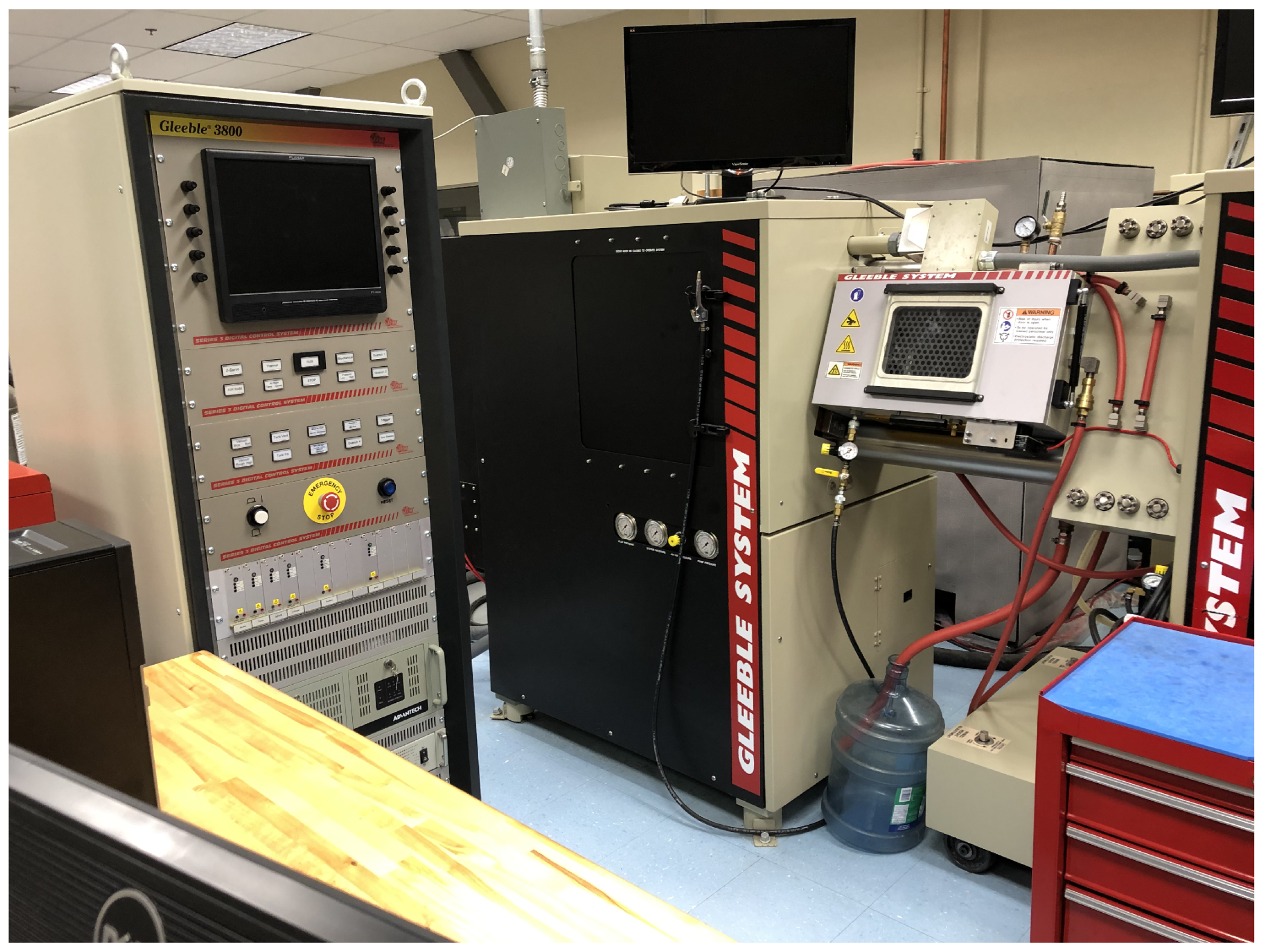
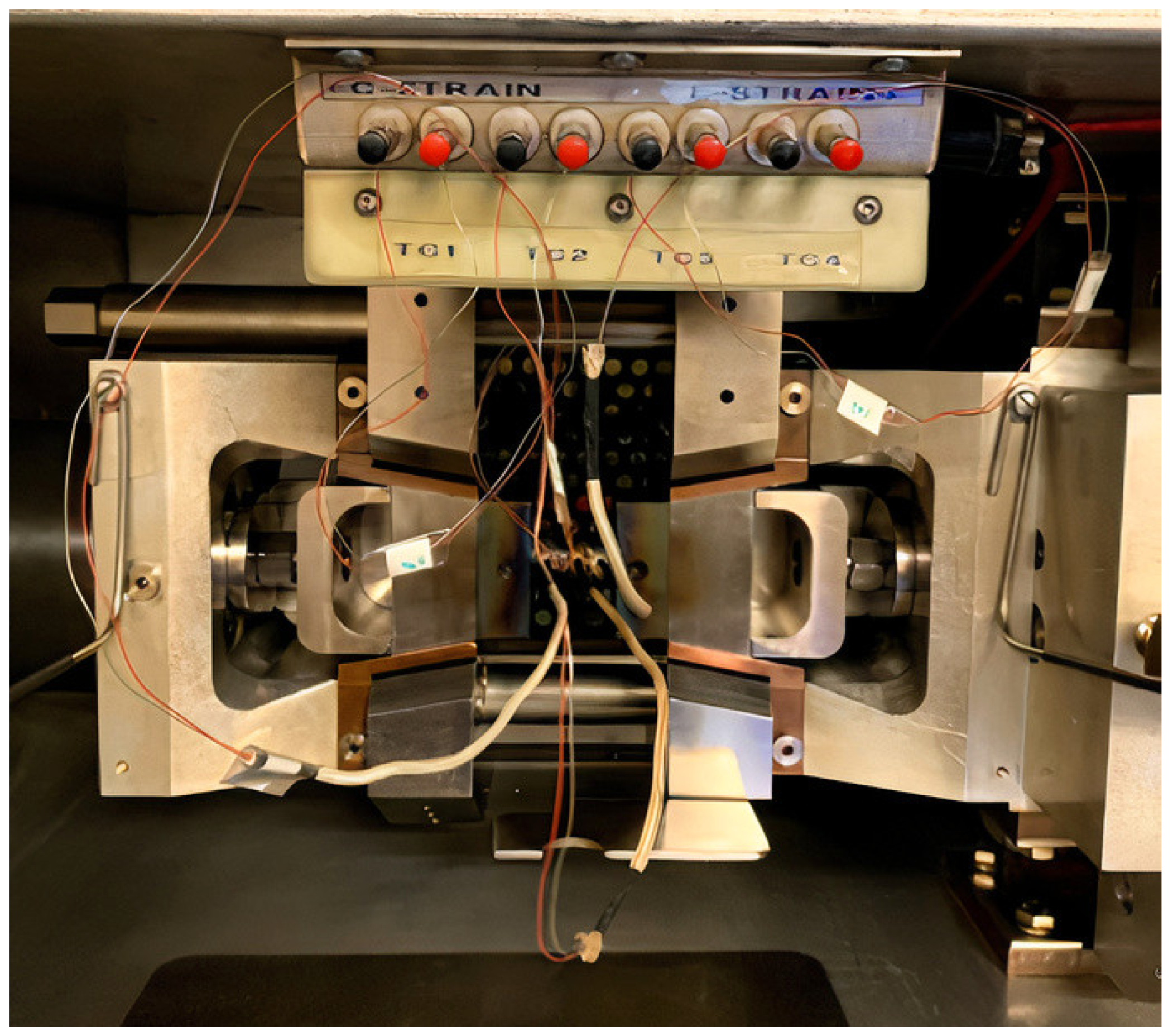
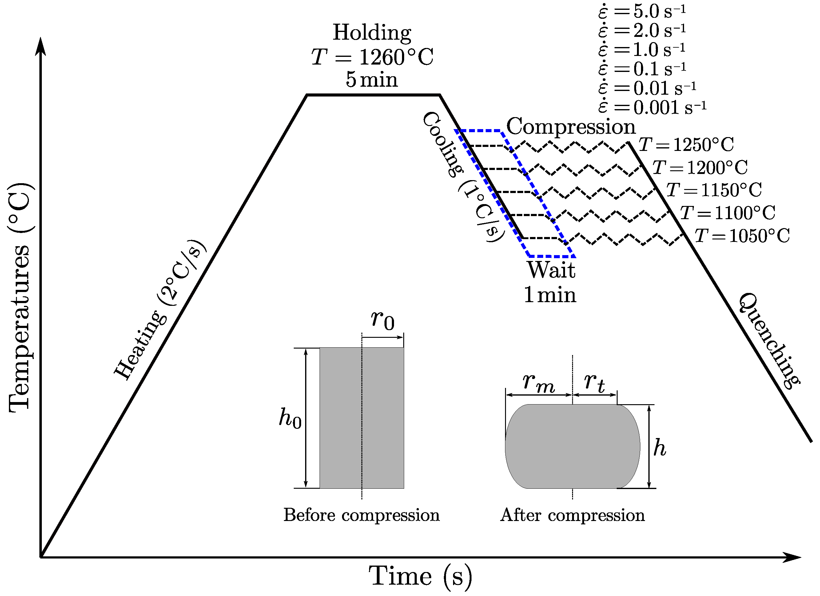
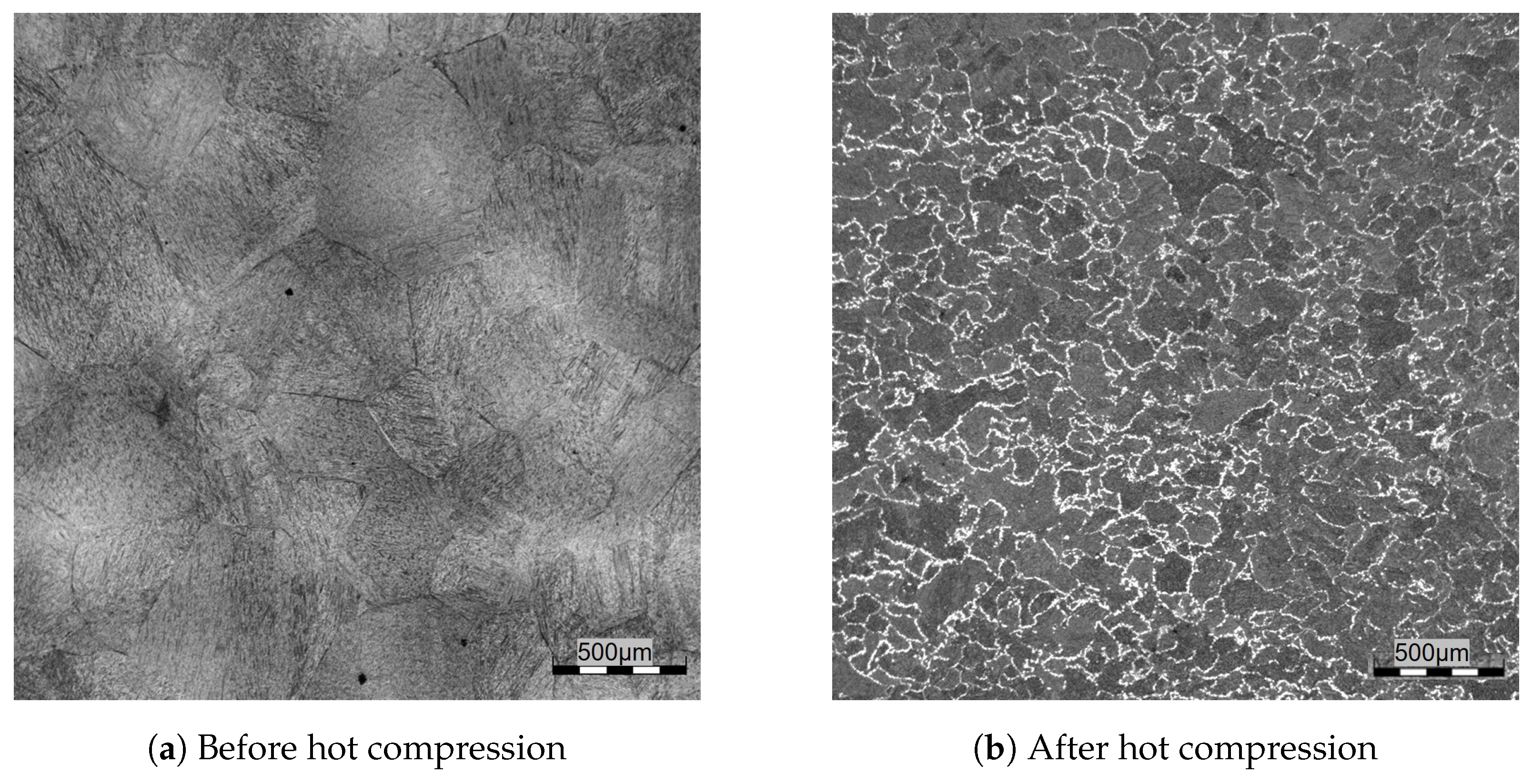
2.1. Experimental Procedure

The material used in this study consisted of a medium carbon steel whose chemical composition is given in Table 1.
Cylindrical samples were machined with an initial diameter of d = 10 mm and a height of h 0 = 15 mm. Hot compression tests were performed on a Gleeble-3800 thermomechanical simulator (see Figure 1), for 5 temperature levels, namely 1050 °C, 1100 °C, 1150 °C, 1200 °C, and 1250 °C, with the 6 strain rates of 0.001 s 1 , 0.01 s 1 , 0.1 s 1 , 1 s 1 , 2.0 s 1 , and 5 s 1 .
Thin tantalum sheets were used as the lubricating material at the contact surface of the anvils and samples to minimize friction during testing. Figure 2 shows the inside of the Gleeble thermomechanical simulator with the specimen in place. We used 3 thermocouples soldered to the specimen to record the temperature history during the test and to ensure that the specimen was at the correct temperature prior to testing.
As shown in Figure 3, the samples were heated to a temperature of 1260 °C with a heating rate of 2 °C/s and held at this temperature for 5 min to eliminate thermal gradients. They were then cooled down with a rate of 1 °C/s to the test temperature and then held at constant temperature for 1 min before deformation. During the compression phase, the temperature of the specimen is kept constant by the thermal control system of the machine. After compression, the specimen is quickly quenched to freeze its microstructure for later analysis. Figure 3 also shows the aspects of the specimens before and after the compression test: h 0 and r 0 are the height and radius before compression and h, r m , and r t are the height, large radius, and small radius of the specimen after compression, respectively.
The stress–strain curves are automatically exported from the Gleeble thermomechanical simulator system as the true stress and true strain according to the L-gauge, where the formula to obtain the curves is given by σ = F / A and ε = ln 1 + Δ h / h 0 or C-gauge, having the following formulas: σ = 4 F / π ( d + Δ d ) 2 and ε = 2 ln d / ( d + Δ d ) with d = 2 r 0 and where F is the force as measured by the Gleeble load cell. As the raw data contain noises, the savgol_filter method from the scipy library was used to remove noise and provide smoother data. To allow further use of the data in numerical simulations, the elastic parts were removed.

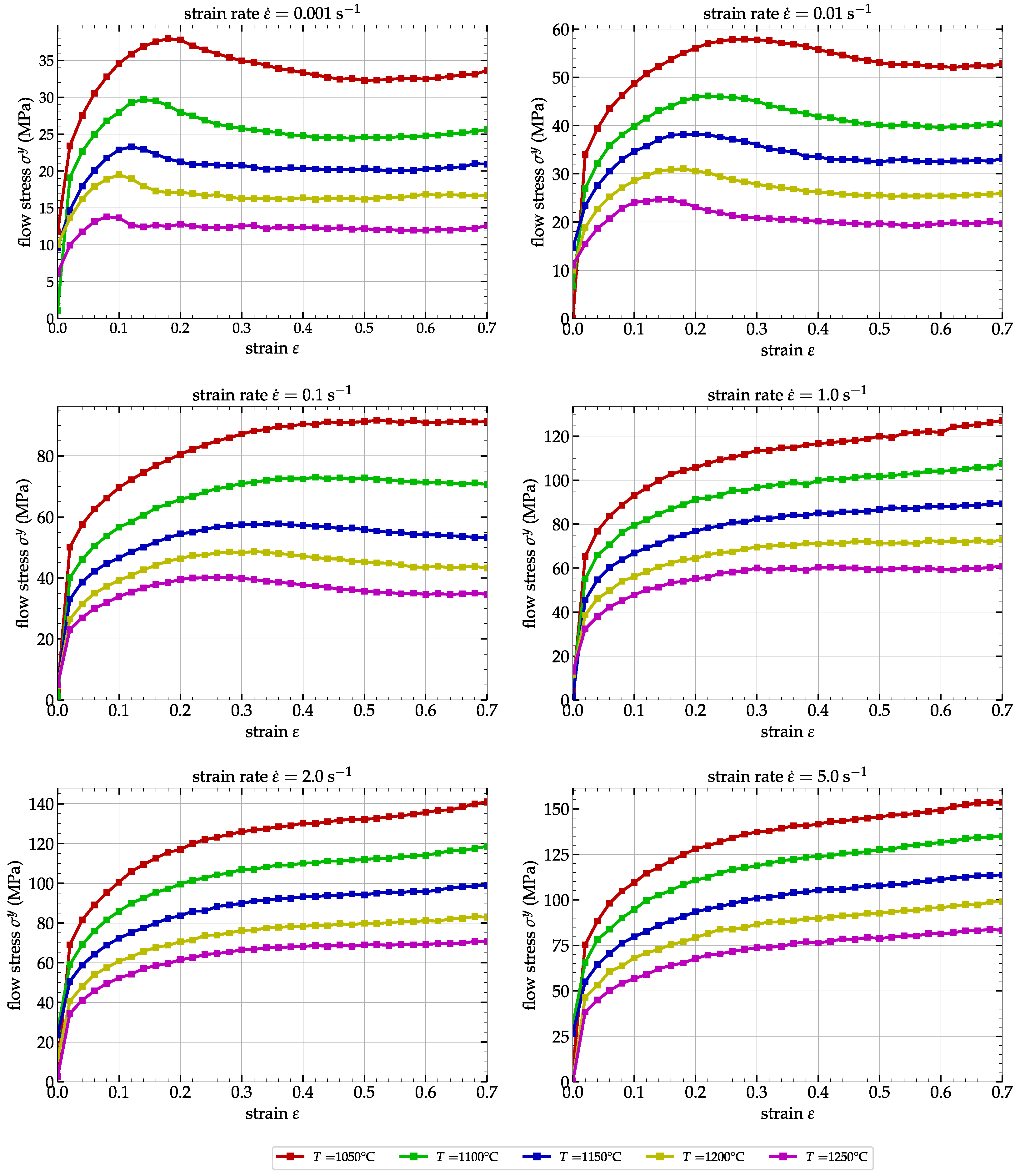
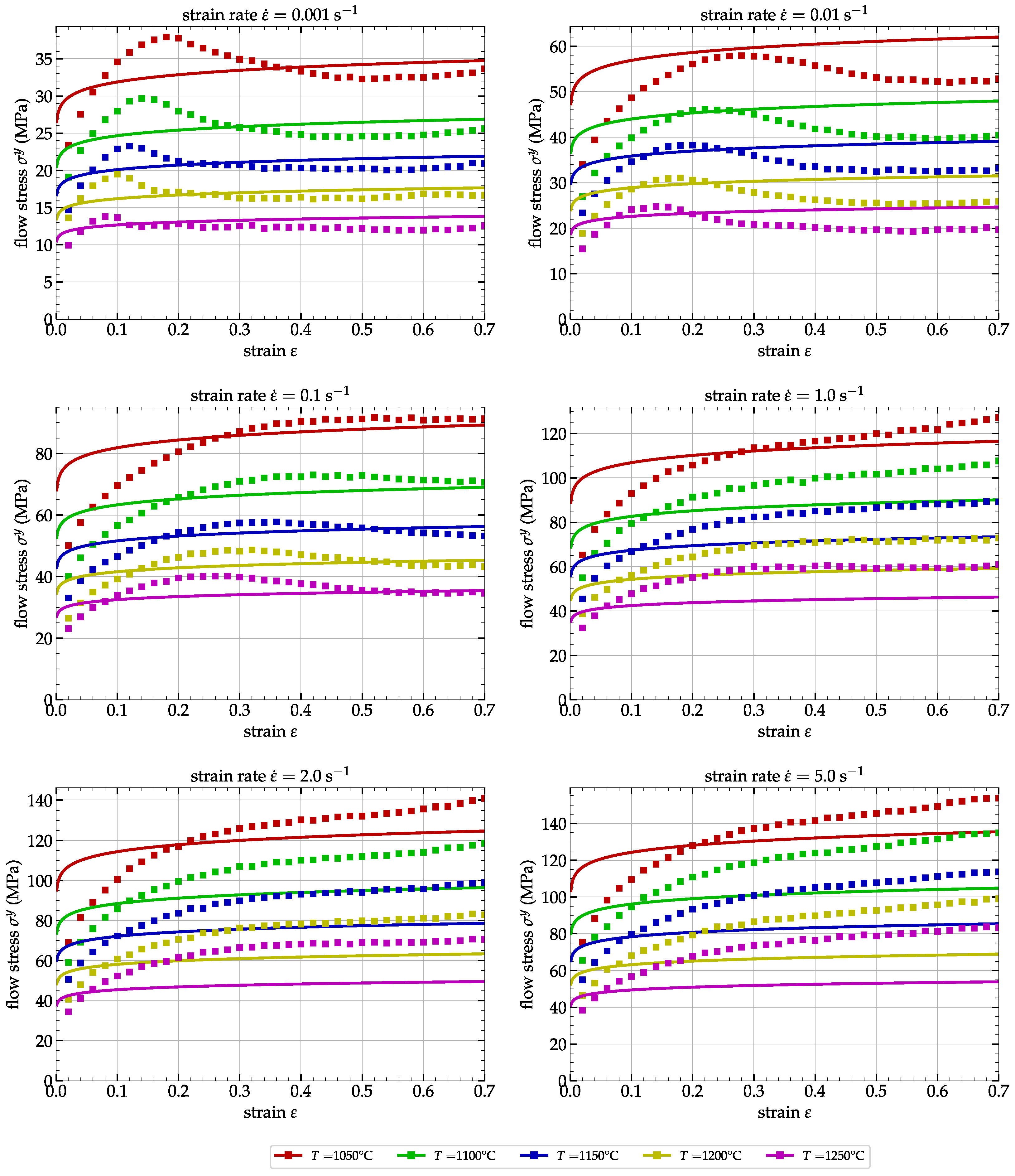
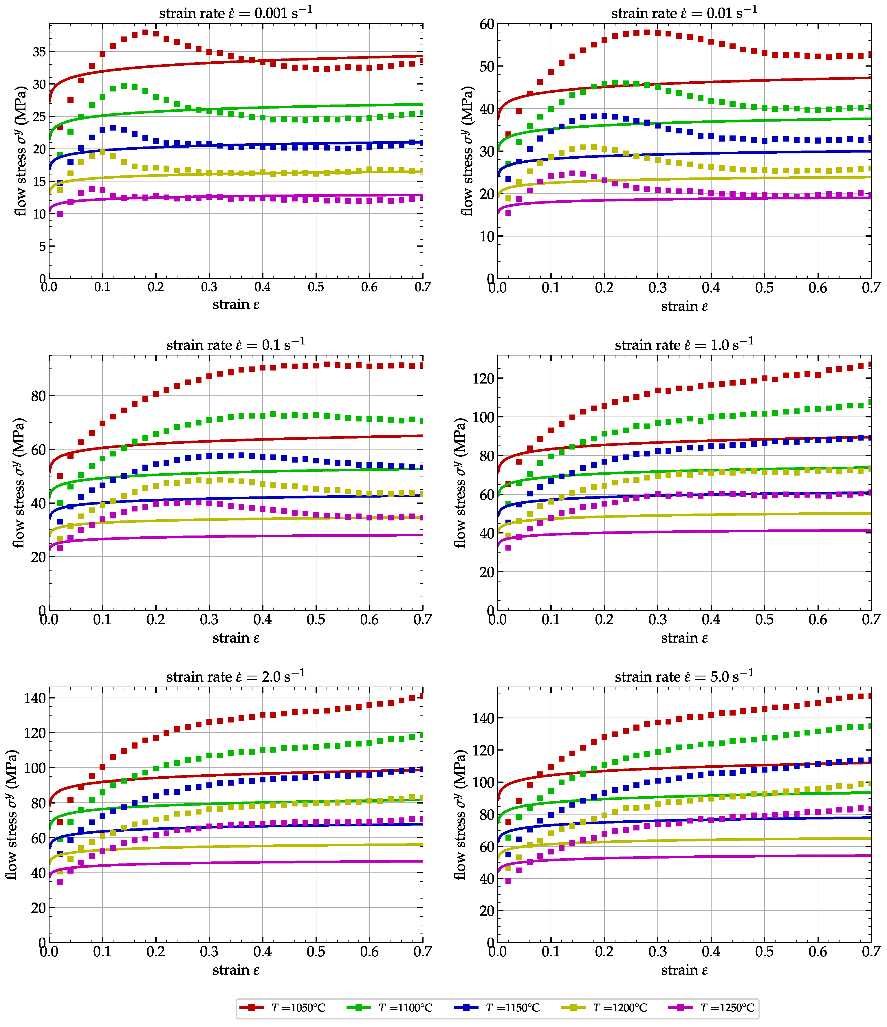
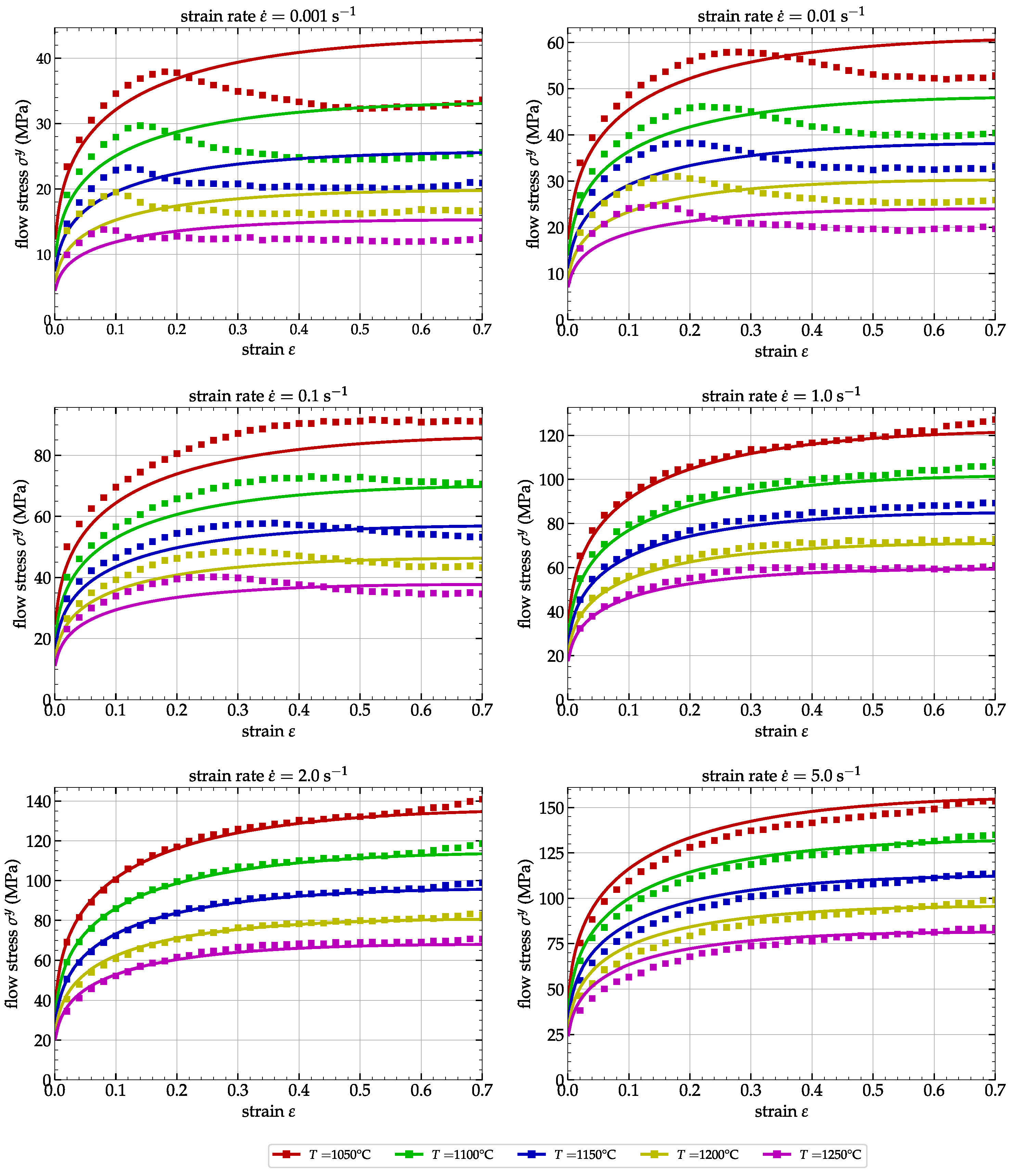
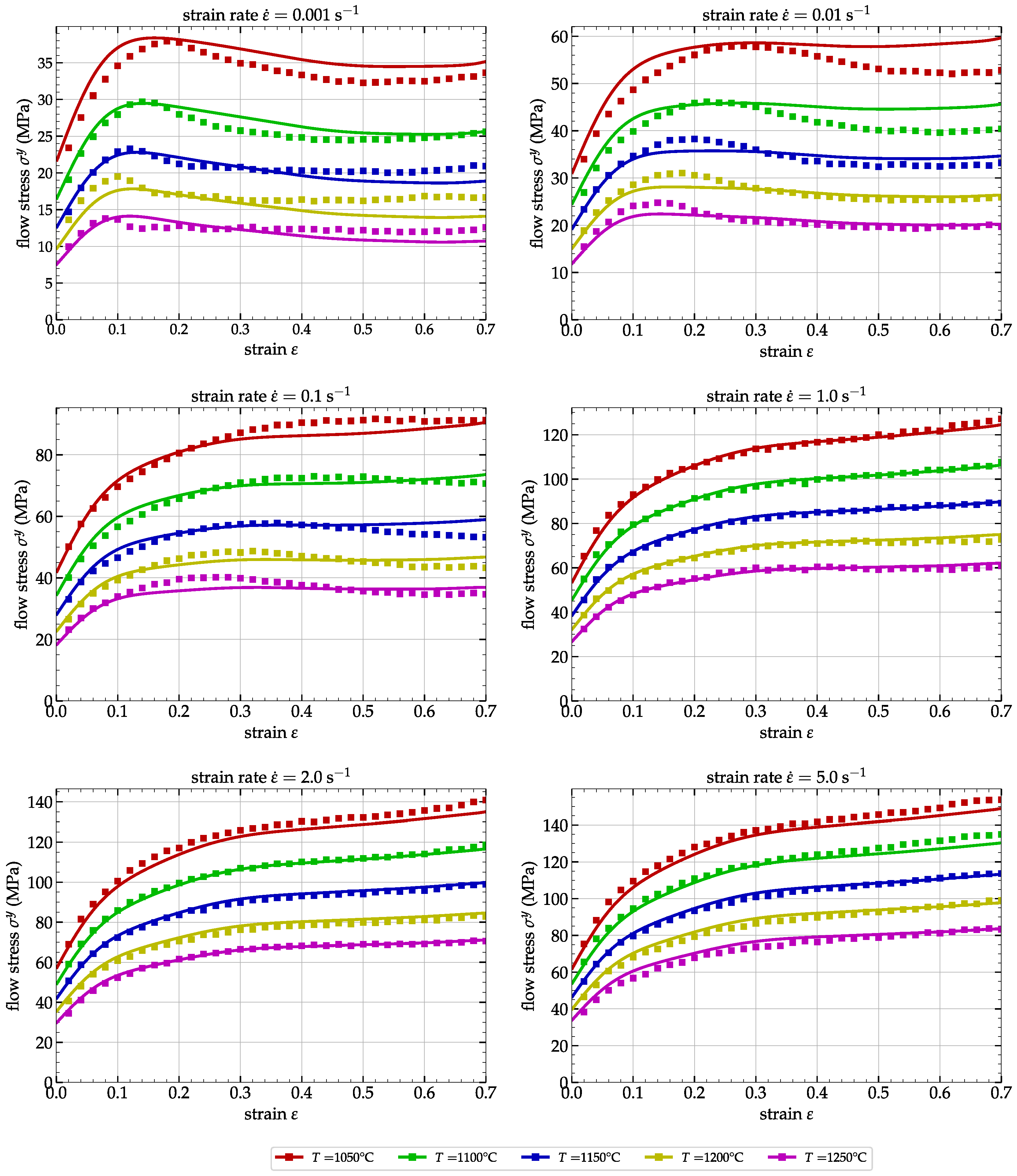
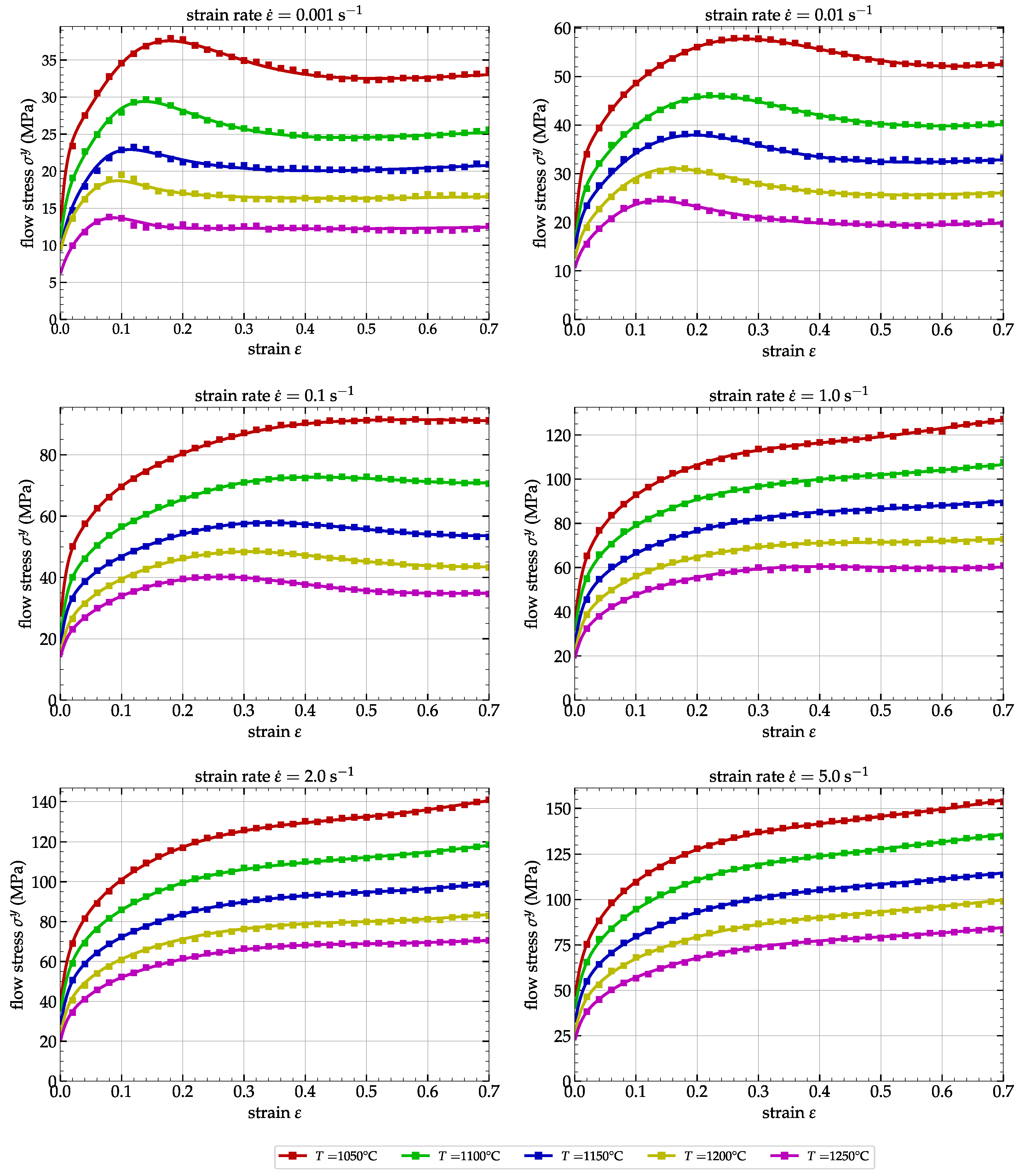
2.2. Compression Tests’ Results

The set of flow stress σ y versus strain ε curves obtained from compression tests performed on the Gleeble-3800 simulator for each test condition (6 strain rates and 5 temperatures) is presented in Figure 4.
All data curves contain 700 equidistant strain values up to ε = 0.7 . Therefore, there are 6 strain rates and 5 temperatures, and the database consists of 21,000 data points. For the identification of the parameters of all the analytical models presented in this article, we restricted the database to 35 strain values between 0.02 and 0.7 , with a step of 0.02 (this is illustrated in Figure 4, where the data used correspond to the dots on the graphs). The overall behavior of these curves shows that the flow stress σ y increases with increasing strain rate ε . , but decreases with increasing temperature T. It should be noted that the strain also influences the flow stress. Indeed, for the lowest strain rates ε . , the flow stress σ y increases with the strain ε until a value of about ε = 0.2 to 0.3 and then decreases to maintain a more or less constant value until the end of the test. For the highest strain rates ( 1 s 1 , 2 s 1 , and 5 s 1 ), the flow stress increases throughout the test. The slight increase in stress at low strain rates, when the strain is large, has been reported to be due to friction between the sample and the anvil during the test [45]. The frictional effect is also visible when testing at low strain rates, as the effect of lubrication decreases over time and friction, thus, increases. The increase of stress observed at the beginning of the deformation and up to 0.1 is due to work hardening (WH). After 0.1 and up to 0.2 , the flow stress shows a continuous reduction with increasing stress until a peak or an inflection of the work hardening rate. This behavior indicates that thermal softening becomes more and more predominant until it exceeds WH. At this step, the stress curve shows three different patterns with the increasing strain: (i) gradual decrease to a steady state with DRV/DRX softening. This is the case for all deformation temperatures and strain rates between 0.001 and 0.1 s 1 , except for those at 1050 °C and 1100 °C; (ii) higher stress levels without significant softening and work hardening at 1050 °C and 1100 °C and a 0.1 s 1 strain rate; (iii) a continuous increase with significant work hardening (all deformation temperatures and strain rate of 1 s 1 ). Therefore, it can be concluded that the softening due to DRX, characterized by a flow curve with a single peak followed by a steady-state flow, takes place at high temperatures and low strain rates. In contrast, at higher strain rates and lower temperatures, the higher work hardening rate slows down the rate of softening due to DRX, and therefore, both the peak stress and the onset of steady-state flow are shifted to higher strain levels. In fact, the drop observed in stress is because of DRX occurrence at all temperatures and strain rates of 0.001 5 s 1 .
Figure 5a shows the microstructure obtained when the sample is held at 1260 °C for 5 min and rapidly cooled to room temperature. From this image, large grains can be observed. On the other hand, Figure 5b shows the microstructure after compression at 1150 °C with a 0.001 s 1 strain rate. To obtain this, the sample is heated up to 1260 °C, then held for 5 min and cooled down to 1150 °C to be held at this temperature for 1 min before compression. After compression, the sample is rapidly cooled to room temperature to preserve the microstructure. From this image, full recrystallization can be observed and is in correlation with Figure 4, where after the peak, a steady stress is observed that describes the end of the recrystallization.
The material is in the single-phase austenite state at all of the test temperatures examined. The data presented in Figure 4 will be utilized in the following section to determine the parameters of the 6 flow laws proposed and to determine which model most closely aligns with the experimental results.

3. Identification of Constitutive Flow Laws’ Parameters

3.1. The Johnson–Cook Model

The JC model, as mentioned above, is one of the most-widely used analytical models because it can be applied to many materials under different conditions of strain ε , strain rate ε . , and temperature T. However, the formulation of this model does not take into account the simultaneous effect of strain, strain rate, and temperature. Indeed, it is formulated by describing the effect of each physical parameter ( ε , ε . , and T) separately as a factor in the mathematical expression of the model, hence its inability to describe the phenomenon of softening induced by temperature. The equation that describes this model is given as follows [17]:
σ y = A + B ε p n 1 + C ln ε . ε . 0 1 T T 0 T m T 0 m ,
where σ y is the flow stress, ε p is the plastic strain, A is the initial elastic limit of the material, B is the strain hardening coefficient, n is the strain hardening exponent, and C and m are the material constants that describe the strain rate hardening coefficient and the thermal softening coefficient, respectively. The other values are reference values: ε . 0 is the reference strain rate; T m and, thus, T 0 are the melting temperature ( 1460 °C in our case) and the reference temperature, respectively. For the determination of the parameters of the analytical models, the reference values for strain rate and temperature are ε . 0 = 0.001 s 1 and T 0 = 1050 °C. In our approach, the reference strain rate and reference temperature for identifying the JC model are the lowest values used during the test; however, sometimes, these values do not always give the best results for the model.
The procedure used to determine the parameters of the Johnson–Cook law is in accordance with the one proposed by Zeng et al. [11]. This method allows sequentially obtaining the 5 parameters in the order A, B, n, C, and m. Thus, according to the experimental data, the initial elastic limit of the material at the reference strain rate ε . 0 and the reference temperature T 0 is A = 13.5143 MPa . For the determination of the constants B and n, from the results of the compression test at T 0 and ε . 0 , these two constants can then be determined by considering only the first term A + B ε p n in Equation (1). Thus, here, B = 21.816 MPa and n = 0.0746 . Once the parameters A, B, and n are known, the determination of C, considering only all the curves at T = T 0 , then gives C = 0.3404 . Finally, the last parameter m is identified from the curves at ε . = ε . 0 and from knowledge of the parameters A , B , C , n and gives m = 0.7057 . All parameters of the Johnson–Cook model are reported in Table 2.
The values predicted by the Johnson–Cook flow law (solid line) and the experimental values (dots) are compared in Figure 6.
The JC model is unable to describe the evolution of the average flow stress for all strain and strain rate levels. The experimental flow stresses show a growth and then a decrease with strain, especially for low strain rates, while the JC model, by its formulation, only allows an increasing evolution of the flow stress σ y as a function of the strain independently of the strain rate value. The discrepancy between the predicted and experimental values is large for low strains and sometimes acceptable for high strains. As expected, the mathematical formulation of the Johnson–Cook flow law is unable to represent the stress drop at low strain rates, with the JC model increasing only monotonically with the strain. Since most of the parameters are identified at low strain rates (A, B, and n), this results in a very poor fit of the model to the experimental data.
The accuracy and predictive ability of the models are usually assessed through certain coefficients such as the mean absolute relative error ( E MAR ) defined by Equation (2):
E MAR ( % ) = 1 N i = 1 N σ i p σ i e σ i e × 100 ,
and the root-mean-squared error ( E RMS ) defined by Equation (3):
E RMS ( MPa ) = 1 N i = 1 N σ i p σ i e 2 ,
where σ i e is the experimental value, σ i p is the value predicted using the given model of the flow stress σ y , and N is the total number of data points used to compute those coefficients (in our case N = 21,000). For the JC model, E MAR = 14.05 % and E RMS = 12.00 MPa . As reported by Phaniraj [46], the correlation coefficient (R) is not always an accurate measure to evaluate the reliability of the constitutive law especially in the case of a highly nonlinear functions because it only shows the correlation of the model with respect to the data and not its accuracy. A good (high) value of R (close to 1) does not necessarily mean a good prediction of the model, but simply establishes a good linearity correlation between the experiment and the prediction; we, therefore, avoided its use in our analysis.

3.2. The Modified-Zerilli–Armstrong Model

The MZA model, which is the modified form of the ZA model, like the JC model presented earlier, is one of the most-widely used models implemented in many FEA codes such as the Abaqus software. The difference between the MZA model and JC model is related to the consideration of the three physical parameters to describe the reality observed from experiments. In the JC model, the parameters are considered separately, while in the MZA model, they are considered simultaneously, and for that formulation, the MZA model is preferred over the JC model [47]. However, the original form of the ZA model has some limitations due to the fact that it is considered as a two-term function (thermal and athermal functions), and to improve the formulation, Samantaray et al. [48] proposed a modified form given by the following equation:
σ y = C 1 + C 2 ε p n exp C 3 + C 4 ε p T T 0 + C 5 + C 6 T T 0 ln ε . ε . 0 ,
where the 7 coefficients C i and n are the parameters of the model to be identified for a given material. To obtain the parameters of the MZA model, we applied the method proposed by [48], and the parameters are summarized in Table 3, while their predictions are plotted in Figure 7.
It can be seen from this figure that both the MZA and JC models are not able to faithfully reproduce the experimental data, especially at low strain rates, but they are slightly better at higher strain rates. The deviation between the predicted values and the experimental values is large because this model has a problem correctly describing the softening in its formulation. For the MZA model, E MAR = 21.20 % and E RMS = 19.57 MPa , showing an overall worse performance than the JC model, as reported in [39]. In addition, it can be observed that, at high strain rates, the MZA model is not good either, even if there is no softening effect, and this can be explained by the fact that this model is formulated for quasi-static phenomena.

3.3. The Hansel–Spittel Model

The Hansel–Spittel model [49] is one of the least-known models in terms of integration in FEA codes, although its parameters can more easily be determined than those of the JC or MZA models. Programming a simple identification script is sufficient to identify its parameters for a given material. The equation of the HS model is given by the following relation:
σ y = A e m 1 T ε m 2 ε . m 3 e ( m 4 / ε ) ( 1 + ε ) m 5 T e m 6 ε ε . m 7 T T m 8 ,
where again, σ y is the flow stress, ε is the strain, ε . is the strain rate, and T is the temperature, as proposed earlier. The coefficients A and m i are the 9 parameters of the model to be identified. However, this model has some shortcomings, notably related to the fact that its accuracy varies according to the number of parameters taken into account during the identification. For its identification, several authors restrict its expression to a reduced number of only 5 or 6 m i parameters, by forcing a zero value for the other parameters [15,18,50].
In the present study, the best results were obtained by taking the model defined by only the first 7 m i terms of the Equation (5), so that m 8 = 0 . From the experimental data obtained during the compression tests, an identification procedure based on the use of the LMFIT optimizer [51] allowed computing the parameters reported in Table 4.
A comparison of the values predicted by the HS model and the experimental values is presented in Figure 8, where the dots represent the experimental values and the solid lines are the values predicted by the Hansel–Spittel flow law. For the HS model, E MAR = 7.75 % and E RMS = 3.80 MPa . It appears that both this model and the previous ones do not adequately predict the experimental one, and the difference is relatively significant for all strain rates below 1 s 1 . This shows that this model is not appropriate for the characterization of this alloy, particularly because of the strong nonlinear behavior observed for low strain rate values. The DRX phenomenon cannot be reproduced by this type of model.

3.4. The Arrhenius Model

The Arrhenius type model [52] is one of the most-used models in the framework of material forming, especially when it comes to studying the material microstructure. The model takes into account the physical phenomena describing the behavior of the material in the formulation of the relationships between the stress σ y , the strain ε , the strain rate ε . , and the temperature T expressed as the power law, exponential law, and hyperbolic sine. This makes it easier to describe the softening phenomenon observed in the material due to increasing temperature. The following equations describe the Arrhenius model:
ε . = A 1 σ y n 1 exp Q R T α σ y < 0.8 A 2 exp ( β σ y ) exp Q R T α σ y > 1.2 A 3 sinh α σ y n 2 exp Q R T for all σ y
with:
Z = ε . exp Q R T ,
where Z is the Zenner–Hollomon parameter [53], ε . is the strain rate ( s 1 ), Q is the apparent activation energy ( J mol 1 ), R is the universal gas constant ( 8.314 J mol 1 K 1 ), T is the absolute temperature (K), σ y is the flow stress (MPa) for a given strain, strain rate, and temperature, and A 1 , A 2 , A 3 , n 1 , n 2 , α , and β = α n 1 are dependent on the material. The corresponding values are independent of the temperature and are obtained from the stress–strain curves at different strain rates and temperatures by the regression method. Combining Equations (6) and (7) allows expressing the flow stress σ y as a function of the Z parameter:
σ y = 1 α ln Z A 1 / n + 1 + Z A 2 / n 1 / 2
To obtain the constitutive equation, all the parameters A, Q, α , and n must be determined for a given material. The strain has a significant nonlinear influence on the behavior of the material by the strain hardening and softening mechanisms at high values of deformation. A strain-dependent factor must, therefore, be taken into account in the Arrhenius model, which leads to the definition of the modified Arrhenius model for which the A, Q, α , and n parameters are expressed as a function of the strain ε by means of polynomial functions of degree m (varying from 1 to 9) of the form:
A ( ε ) = exp ln A 0 + ln A 1 ε + ln A 2 ε 2 + ln A 3 ε 3 + + ln A m ε m
Q ( ε ) = Q 0 + Q 1 ε + Q 2 ε 2 + Q 3 ε 3 + + Q m ε m
α ( ε ) = α 0 + α 1 ε + α 2 ε 2 + α 3 ε 3 + + α m ε m
n ( ε ) = n 0 + n 1 ε + n 2 ε 2 + n 3 ε 3 + + n m ε m
The determination of the order m of the polynomials defining Equations (9)–(12) depends on the ability of the model to represent the nonlinear dependence of the stress on strain and its generalization. The values ln A i , α i , n i , and Q i ( i = 0 , 1 , 2 , 3 , , m ) are the coefficients of the polynomials used to determine using a regression method. Setting m = 9 gives the best results, and the corresponding parameters are reported in Table 5.
This modified form of the Arrhenius behavior law allows an accurate and reliable prediction over a wide range of temperatures and strain rates. Equation (13) is finally used to compute the flow stress σ y from the strain ε , the strain rate ε . , and the temperature T:
σ y = 1 α ( ε ) ln ε . exp Q ( ε ) R T A ( ε ) 1 n ( ε ) + 1 + ε . exp Q ( ε ) R T A ( ε ) 2 n ( ε ) 1 2
Figure 9 shows a comparison of the values predicted by the Arrhenius model and the experimental values. The difference between the experimental and predicted values is small. However, for the strain rate ε . = 0.01 s 1 and for the two low temperature values, the AR model is unable to predict the softening. For the AR model, E MAR = 3.56 % and E RMS = 2.18 MPa .

3.5. The PTM Model

The PTM model [39] is a generalized formulation of the MZA model presented in Section 3.2. When establishing its formulation, the main shortcomings of the MZA model were taken into account, in order to render the PTM model flexible for any type of material studied because it removes the need for a limited number of parameters as in the MZA model. Its construction is based on the use of polynomial functions, as is the case in the AR model. Thus, the physical parameters’ dependent intrinsic functions of the PTM model allow adjusting the model according to the degree selected for each of the 4 constituent polynomials, which provides a good fit for each function. The equation describing the PTM model is, therefore, given by:
σ y = i = 0 q A i ε p i exp j = 0 r B j ε p j T T 0 + k = 0 s l = 0 t C k l ε p l T T 0 k ln ε . ε . 0
where A i , B j , C k l are the parameters (Table 6) of the model to be identified using the procedure proposed in [39]. Quantities q, r, s, and t define the degree of the polynomials used to describe the behavior of the material. The larger these quantities, the greater the number of parameters that need to be identified for the PTM model. The determination of the parameters of this model was performed thanks to the LMFIT Python library [51] (for more details about this model, we refer the reader to our previous work [39]). Thus, all the parameters of this model were calculated with q = 5 , r = 5 , s = 1 , and t = 5 .
Figure 10 presents a comparison of the values predicted by the PTM model and the experimental values. The PTM model is suitable for describing the flow behavior of medium carbon steel, but for the two strain rates ε . = 0.01 s 1 and ε . = 0.1 s 1 , the prediction is not very good. The deviation between the predicted values and the experimental values for other strain rates is relatively low. For the PTM model, E MAR = 4.79 % and E RMS = 4.59 MPa , which is an overall worse performance than the AR model.

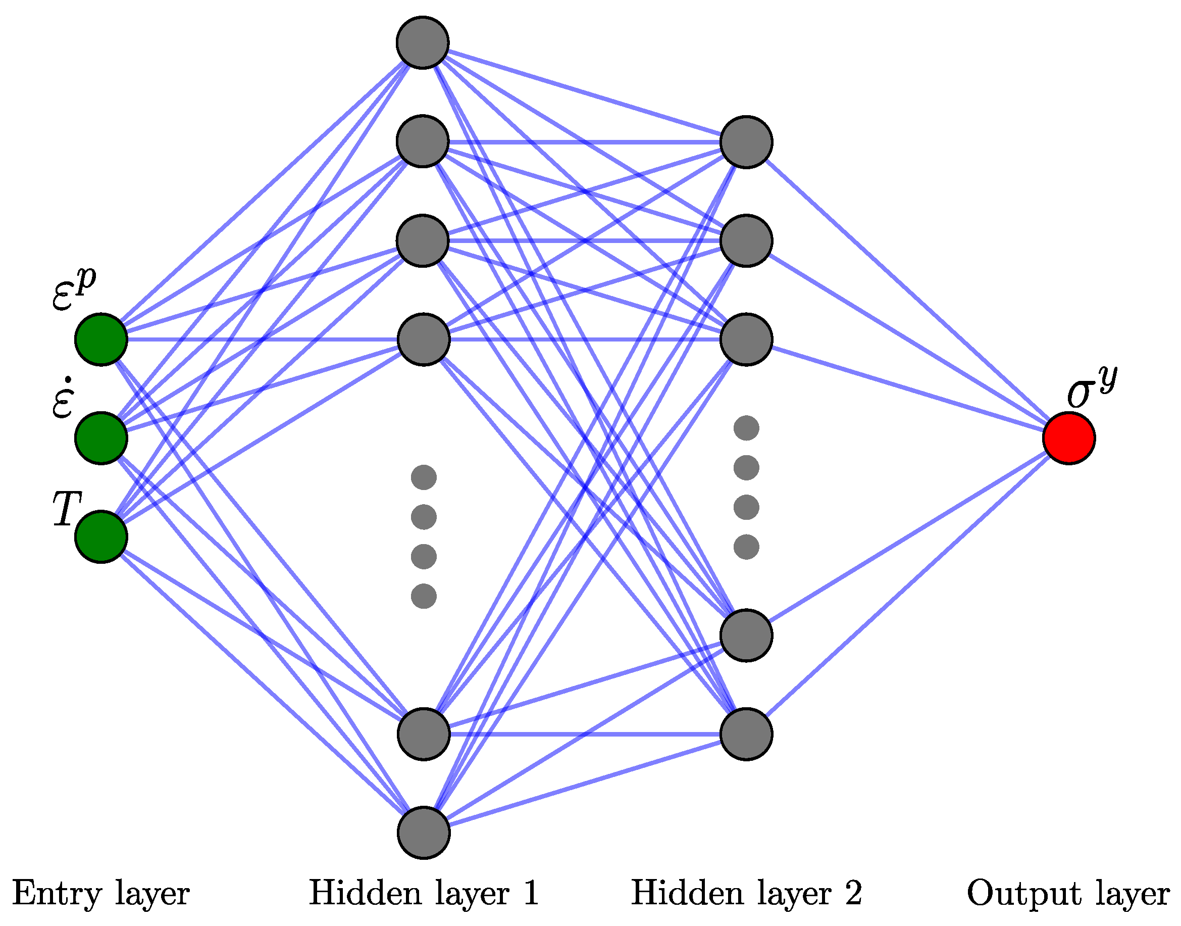
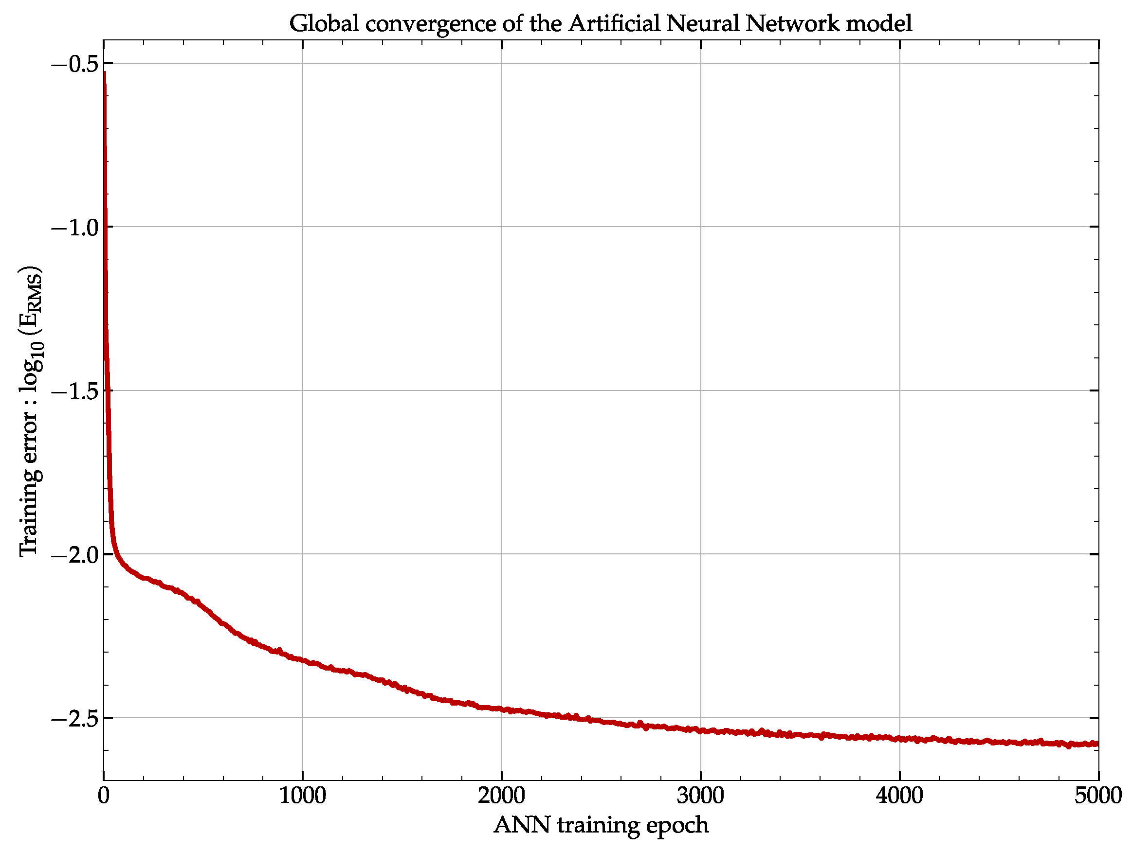
3.6. The Artificial Neural Network Model

Because of their predictive capacity and adaptability, artificial neural networks (ANNs) are increasingly widely used today in many scientific fields. Their operation is based on a training process, during which the principle of minimizing the error between the model’s output and the training data allows the adjustment of the model’s parameters, as in any machine training process.
Neural networks generally have two uses: classification and regression. The first is the ability to classify data into different groups, for example to distinguish between images of cats and dogs. The second corresponds to the universal approximation capacity of these neural networks, which is of interest to us herein, and thus, to the ability, after training, to predict the flow stress σ y values according to the input data, akin to what is achieved by the above-identified analytical models. The main difference is that this approximation is not linked to a fixed mathematical formulation (as in the JC, MZA, AR, HS, and PTM analytical models), but is only dependent on the data used for training, the number of layers, the number of neurons per layer, and the activation functions associated with the neurons of the network. A feed-forward ANN, as used in our application, contains an input layer, an output layer, and a number of hidden layers (2 in our case). Each layer of neurons is connected to the one before it and the one after it by weighted connections. Thus, all the neurons of the k t h layer are connected to all the neurons of the ( k 1 t h ) layer, as shown in Figure 11.
Any hidden layer k, containing n neurons, takes a weighted sum of the outputs y ^ of the immediately preceding layer ( k 1 ) , containing m neurons, given by the following equation:
y i ( k ) = j = 1 m w i j ( k ) y ^ j ( k 1 ) + b i ( k ) ,
where y i ( k ) is the entry of the ith neuron of layer k, y ^ j ( k 1 ) is the output of the jth neuron of layer ( k 1 ) , w i j ( k ) is the associated weight parameter between the ith neuron of layer k and the jth neuron of layer ( k 1 ) , and b i ( k ) is the associated bias of the ith neuron of layer k. Those weights w i j and bias b i , for each layer, are the training parameters of the ANN, which we have to adjust during the training procedure described in Pantalé et al. [16,44]. For the proposed model, we selected the Sigmoid activation function, so that each neuron in the hidden layer k provides an output value y ^ from the input value y of the same neuron defined by Equation (15) according to the following equation:
y ^ = 1 1 + e y
No activation function was used for the output neuron of the ANN as usually done in a regression ANN.
After some tests of different types of network architectures and in accordance with previous works, a network structure with two hidden layers including 15 neurons for the first hidden layer and 7 neurons for the second layer gave the best compromise between prediction, training time, and model compactness. From a global architecture point of view, the input layer is composed of 3 neurons ( ε p , ε . , T) and the output layer is composed of a single neuron corresponding to the σ y flow stress. This architecture leads to a global model with 180 parameters to be identified (60 for the first layer, 112 for the second layer, and 8 for the output layer).
The Python program used for training the neural network was developed using the specialized Python library, Tensorflow [54]. The Adaptive Moment Estimation (ADAM) optimizer [55] was used for the training phase. The training data were those from the tests presented in Section 2.2 and were composed of 21,000 quadruplets of ( ε p , ε . , T, σ y ) values. The training was performed on the basis of 5000 epochs of the experimental dataset. It took 40 min of training on a Dell XPS-13 7390 laptop running Ubuntu 22.04 LTS 64 bits with 16 GB of RAM and an Intel 4-core i7-10510U processor to obtain the converged parameters of the ANN model. Figure 12 shows the evolution of the training error defined by the log 10 of the E RMS during the training phase.
As can be seen in this figure, after 5000 epochs, we can consider that we have reached a stationary state of the model training, such that it is useless to continue with the training phase.
Once the training phase is over, the trained model can be used to predict the behavior of the medium carbon alloy as a function of the input data, similarly to what was done with the analytical models. One can either use the model directly by providing it with new input data or retrieve the 180 parameters identified during the training and inject them into a mathematical model based on Equations (15) and (16), which can be implemented in any language (e.g., in FORTRAN for use on the Abaqus Explicit FEA code), as proposed in Pantalé et al. [16,44]. For compactness, the parameters of the ANN model and the complete procedure to compute the flow stress σ y from the input data are provided in Appendix A.
As for the above-considered analytical models, Figure 13 shows a comparison between the flow stresses predicted by the ANN model and the data measured during the hot compression test.
The experimental data and the ANN prediction correlate very well over the entire range of data, and the predicted data can track the hardening and softening regions of the hot deformed material well. For the ANN model, E MAR = 0.62 % and E RMS = 0.38 MPa , which is excellent. This model can be used to simulate the hot deformation of this type of alloy with much greater reliability with respect to the actual material behavior than the analytical models presented in the above sections.

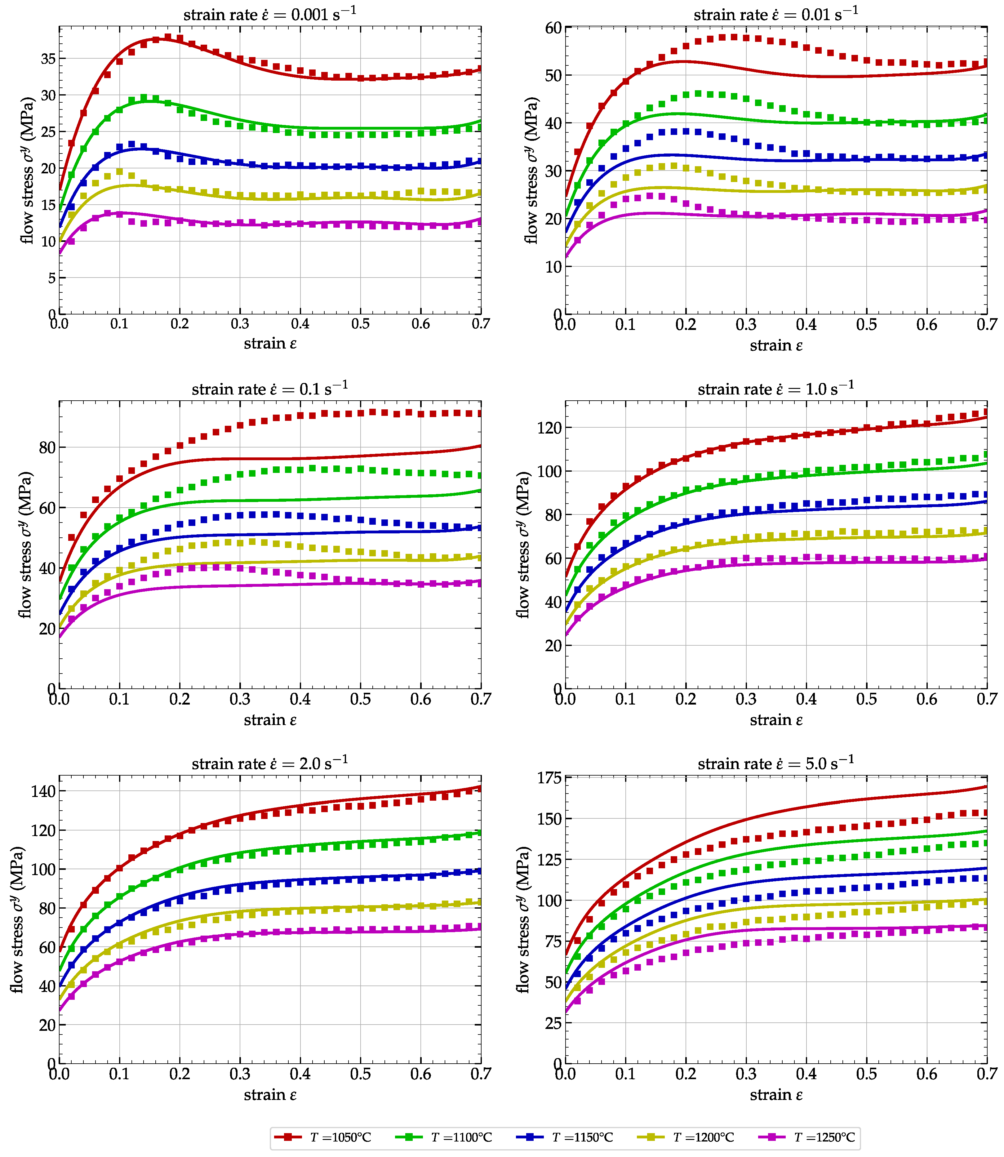
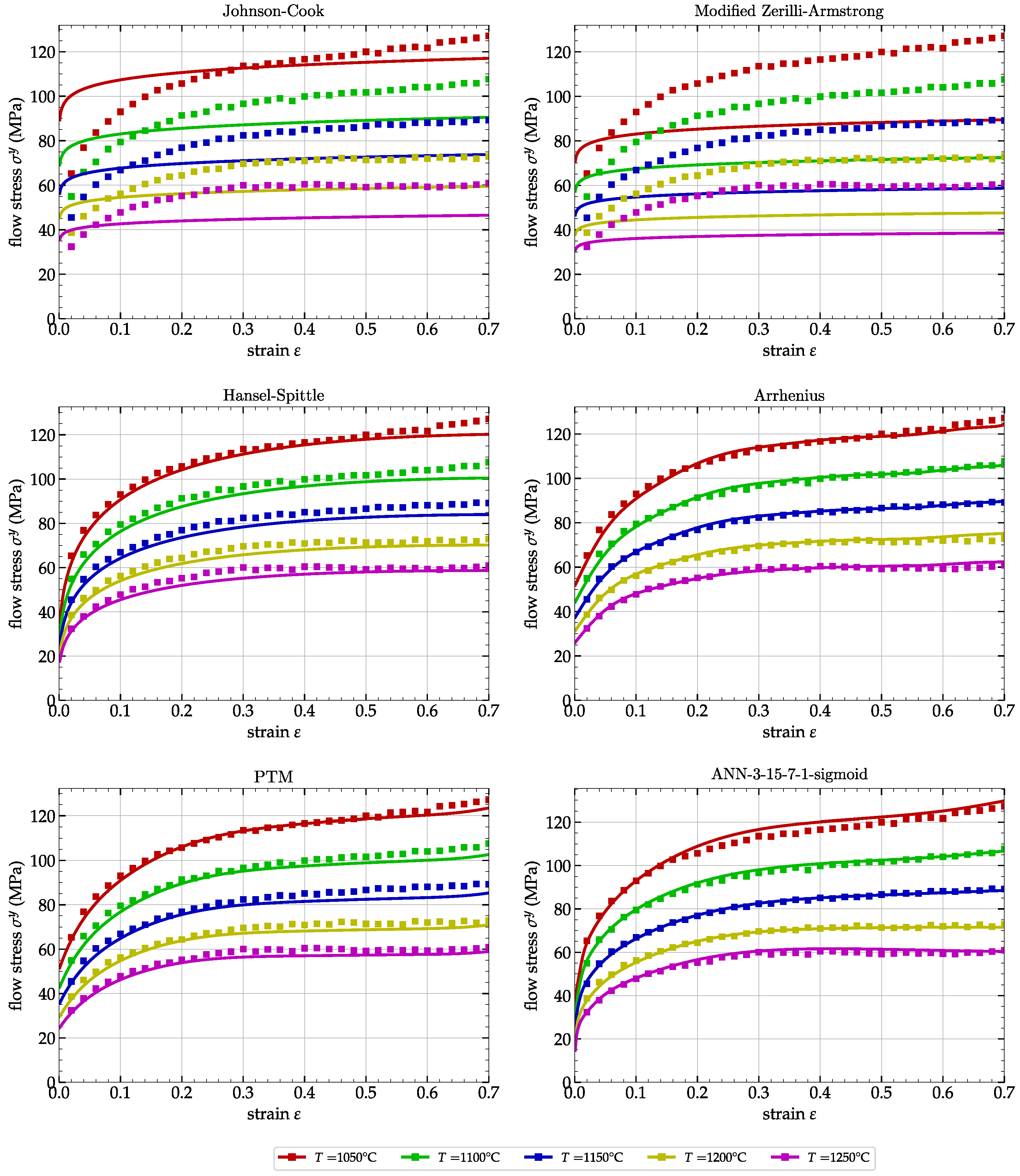
3.7. Comparison of Analytical and ANN Models

A summary of the coefficients for evaluating the high-temperature flow stress prediction capability of the medium carbon alloy for all models presented in this work is reported in Table 7.
From Table 7, we can see that the ANN model has a much better predictive capacity than all the analytical models presented in the above sections. Globally, the values of E MAR and E RMS are six-times lower than with the best of the analytical models, i.e., the Arrhenius model, quoted as reference in the context of the hot forming of alloys [56].
The ANN, Arrhenius and PTM models are the only models that take into account softening with the deformation of medium carbon at a low strain rate, unlike the other three models, which only present an increase in the flow stress with the strain, irrespective of the strain rate and temperature, hence their poor performance in predicting the behavior of this material and, more particularly, at low strain rates. The parameters reported in Table 7 and the correlations that can be seen in Figure 6, Figure 7, Figure 8, Figure 9 and Figure 10 and Figure 13 allow concluding that the ANN model is the most efficient of all the models presented when it comes to describing the behavior of the medium carbon alloy for high-temperature deformation applications.

4. Interpolation and Extrapolation Capability of Models

In order to better compare the performances of the above analyzed models (the five analytical models and the ANN based model), in this section, we present the ability of each of these models to interpolate and extrapolate the results as a function of the strain rate ε . . The identification of the above-analyzed models was based on a set of experimental data corresponding to six strain rates, five temperatures, and strains ranging from 0 to 0.7 . To test the training capacity and reliability of these models, we propose here to perform the training of the models on only five strain rates by voluntarily omitting the strain rate ε . = 1 s 1 or ε . = 5 s 1 .
Thus, one of the omitted strain rates ( ε . = 1 s 1 ) is within the range of strain rates for model identification ( 0.001 s 1 to 5 s 1 ), and therefore, we can test the ability of the models to interpolate the results from the other five strain rates and be able to quantify any deviation from experimental values. On the other hand, since the omitted strain rate ( ε . = 5 s 1 ) is outside the range of strain rates for the model identification ( 0.001 s 1 to 2 s 1 ), we tested the ability of the models to extrapolate the results and quantify deviations with the experimental values.

4.1. Interpolation Validation

For interpolation validation, the chosen omitted strain rate was ε . = 1 s 1 , and those used for identification (or training for the ANN) were the five others, i.e., ε . = [ 0.001 , 0.01 , 0.1 , 2 , 5 ] s 1 . All models were re-identified from the same experimental data on a dataset corresponding to five strain rates and five temperatures.
Figure 14 shows a comparison, for the strain rate ε . = 1 s 1 , of the flow stresses σ y calculated by the models (as a line) and the experimental results (as dots) for the five analytical models and the neural network.
Table 8 shows the E MAR and E RMS deviations between the different models and the experimental data calculated either for the five identified strain rates (lines referred as id. ε . ), the six strain rates (lines referred as all ε . ), or only on the strain rate ε . = 1 s 1 .
In Figure 14, it can be seen that the first two models (JC and MZA) presented in this study do not have the ability to reproduce the behavior of the material for the strain rate ε . = 1 s 1 . Overall, the JC model gives better results than the MZA model for ε . = 1 s 1 , which is reflected in Table 8 by a lower value of the E MAR and E RMS for the JC than for the MZA model. Nevertheless, these values are higher than 10 % for the JC model and 20 % for the MZA model, which reflects the poor ability of these models to correctly model the behavior of this material. This finding is in agreement with the previous findings of Section 3.1 and Section 3.2, which showed the inability of these models to take into account the softening of the behavior visible at low strain rates and low temperatures.
From a general appearance point of view, the other four models, HS, AR, PTM, and ANN, give globally similar results, with a higher reliability for the AR and ANN models compared to the other two models. Table 8 shows a quantitative comparison of the E MAR and E RMS for three different cases: the 5 identified strain rates, only the strain rate ε . = 1 s 1 , and all 6 strain rates for these six models. It appears from this table that, while the two models, AR and ANN, give equivalent (and excellent) results concerning the values of the E MAR and E RMS for the strain rate ε . = 1 s 1 , the ANN model gives a globally better result across the entire strain rate spectrum, with values of E MAR = 0.96 % and E RMS = 1.18 MPa , respectively, that is to say, values that are approximately 2- to 3-times lower for the ANN model than for the AR model.
This shows the superior reliability of the ANN model over the five analytical models presented in this study both in terms of the interpolation capability of the model and of the overall behavior.

4.2. Extrapolation Validation

For the validation of the models’ ability to extrapolate, the omitted strain rate chosen was ε . = 5 s 1 and those used for identification were ε . = [ 0.001 , 0.01 , 0.1 , 1 , 2 ] s 1 . The strain rate omitted in this analysis, therefore, has the highest value, which restricts the training domain.
In this new identification configuration, Figure 15 shows a comparison, for strain rate ε . = 5 s 1 , of the flow stresses σ y computed by the models (as a line) and the experimental results (as dots) for the five analytical models and the neural network.
Table 9 shows the E MAR and E RMS deviations between the different models and the experimental data calculated either for the 5 identified strain rates (lines referred as id. ε . ), the 6 strain rates (lines referred as all ε . ), or only on the strain rate ε . = 5 s 1 .
As presented in the previous section regarding the interpolation capability of the models, in Figure 15, it can be seen that the first two models, JC and MZA, in this study again do not have the ability to correctly reproduce the material behavior for the strain rate ε . = 5 s 1 . The JC model performs better than the MZA model for ε . = 5 s 1 , which is reflected in Table 9 by a lower value of the E MAR and E RMS for JC than for MZA. Nevertheless, these values are too large for proper use. Once again, it is the inability of these models to take into account the softening of the behavior at low strain rates and low temperatures that is at the origin of these values.
The other four models, HS, AR, PTM, and ANN, give better results with higher reliability for the AR and ANN models than for the other two models. Table 9 shows a comparison over all strain rates and over ε . = 5 s 1 for these six models. The HS model performs worse in extrapolation than the AR and ANN models, while the PTM model is relegated to the last position in this ranking with values of the E MAR and E RMS greater than 10 % for the strain rate ε . = 5 s 1 . The two models, AR and ANN, give the best results for the values of the E MAR and E RMS for the strain rate ε . = 5 s 1 . This time, the AR model performs a little better on the ε . = 5 s 1 strain rate as compared to the ANN model, but the latter gives a globally better result across the entire strain rate spectrum, with values of E MAR = 1.09 % and E RMS = 2.40 MPa , respectively.
We can, therefore, conclude from this part of the study that the AR model is the best-performing of the five analytical models presented, which is in agreement with the fact that it is widely used for thermomechanical processing, but the ANN model approach has advantages over the AR model approach in that, overall, the ANN model is more faithful to the experimental data than is the AR model, for all strain rates.

5. Conclusions

Experimental tests were performed on a Gleeble thermomechanical simulator for a modified medium carbon alloy to investigate the applicability and predictive accuracy of five analytical models and an artificial neural network model over a range of strains (0.0–0.7), strain rates (0.001 s 1 –5 s 1 ), and temperatures (1050 °C–1250 °C). The analytical models selected for this study were the Johnson–Cook (JC) model [17], the Modified-Zerilli–Armstrong (MZA) model [48], the Hansel–Spittle (HS) model [49], the Arrhenius (AR) model [52], and the PTM model [39]. The ANN model selected was the one introduced by Pantalé et al. [16]. An analysis of the data from the Gleeble trials and a comparison of the six models proposed in this study against the experiments led to the following conclusions.
From an experimental point of view, it appeared from the tests carried out that the flow stress σ y increased with a decrease of the temperature T and an increase of the strain rate ε . due to the competitive appearance of the dynamic softening and work hardening mechanisms. The dynamic recrystallization (DRX) phenomenon, introduced through the difference between the maximum and permanent strains, showed a partially complete microstructure evolution. Thus, at high strain rates, it is difficult to visualize the DRX phenomenon on the flow curves due to the sensitivity of this phenomenon to the strain rate. A study focused on an in-depth analysis of the microstructure of this steel alloy, and its impact on mechanical properties is currently underway.
Five analytical models and an artificial-neural-network-based model were identified for this alloy. Among the analytical models, the JC and MZA models proved inadequate to reproduce the behavior of this material, while the HS, PTM, and AR models showed their capabilities, presenting an acceptable E MAR error (from 3.5 % to 7.7 % ). The AR model (with a 3.56 % error) proved superior to the other two, thus justifying its use in thermomechanical processes. The ANN model was largely more accurate than the analytical models in predicting the flow stress σ y of medium carbon, with an E MAR = 0.62 % .
To test the performance of each proposed model, a study was conducted to evaluate the interpolation and extrapolation capability of the developed models. In the case of interpolation, the HS, PTM, and AR models correlated well with the experiment, but the ANN model was superior, with an error factor five-times lower than the AR model. For data extrapolation, the HS, PTM, and AR models again correlated well with the experiment, but the ANN model once again performed better globally.
Identifying the parameters of an ANN model from experimental data requires more time than identifying the parameters of analytical models (about 40 minutes on a working laptop), but as shown by Pantalé et al. [16,44], implementing an ANN model in a computational code is straightforward.

Author Contributions

Conceptualization, P.T.M. and O.P.; methodology, O.P.; software, P.T.M. and O.P.; validation, O.P.; formal analysis, O.P.; investigation, P.D.; resources, P.D. and M.J.; data curation, P.T.M. and P.D.; writing—original draft preparation, P.T.M.; writing—review and editing, O.P.; visualization, O.P.; supervision, M.J., A.T. and O.P.; project administration, M.J.; funding acquisition, M.J. All authors have read and agreed to the published version of the manuscript.

Funding

This work was supported by the Natural Sciences and Engineering Research Council of Canada (NSERC) in the framework of a Collaborative Research and Development project (CRD) (Grant Number 5364418).

Data Availability Statement

The raw/processed data required to reproduce these findings cannot be shared at this time due to privacy and ethical concerns.

Acknowledgments

The authors acknowledge Jean-Benoit Morin, Director of Metallurgy and Quality from Finkl Steel-Sorel, Abdelhalim Loucif from the R&D department of Finkl Steel-Sorel, Ecole de Technologie Superieure, and Ecole Nationale d’Ingenieurs de Tarbes, France, for providing technical data, materials, and testing facilities.

Conflicts of Interest

The authors declare no conflict of interest.

Abbreviations

The following abbreviations are used in this manuscript:
ANNArtificial neural network
ARArrhenius
CPUCentral processing unit
DRVDynamic recovery
DRXDynamic recrystallization
FEAFinite element analysis
HSHansel–Spittel
JCJohnson–Cook
MZAModified-Zerilli–Armstrong
WHWork hardening
ZAZerilli–Armstrong

Appendix A

We report hereafter the computing process and the 180 coefficients of the artificial neural network ANN-3-15-7-1-sigmoid model used in Section 3.6. In order to use this model, we describe hereafter the details of the procedure to compute the flow stress σ y from the input variables ε p , ε . , and T. This process can be decomposed into three phases:
  • We first have to normalize the input values of the ANN x i within the range [ 0 , 1 ] to avoid an ill-conditioned system, as presented by many other authors in the literature [41,57]. Therefore, the three components of the input vector x are obtained from the plastic strain ε p , the plastic strain rate ε . p , and the temperature T using the following expressions:
    x = x 1 = ε p [ ε p ] m i n [ ε p ] m a x [ ε p ] m i n x 2 = ln ( ε . / ε 0 . ) [ ln ( ε . / ε 0 . ) ] m i n [ ln ( ε . / ε 0 . ) ] m a x [ ln ( ε . / ε 0 . ) ] m i n x 3 = T [ T ] m i n [ T ] m a x [ T ] m i n
    where [ ] m i n and [ ] m a x are the boundaries of the range of the corresponding field: ε p 0.0 , 0.7 , ε . 0.001 s 1 , 5.0 s 1 , T 1050   ° C , 1250   ° C , and σ [ 1.311 MPa , 153.739 MPa ] . The reference strain rate is ε 0 . = 0.001 s 1 .
  • Then, we compute the output s of the ANN from the input vector x using the following three equations:
    y 1 = 1 + exp w 1 · x b 1 1
    y 2 = 1 + exp w 2 · y 1 b 2 1
    s = w T · y 2 + b
  • Finally, the flow stress σ y can be obtained from the output s of the ANN using the following equation:
    σ y = [ σ ] m a x [ σ ] m i n s + [ σ ] m i n
Conforming to the computing process proposed by Equations (A1)–(A5), we report hereafter the 180 coefficients of the ANN-3-15-7-1-sigmoid model used in Section 3.6. The weight matrix for the first hidden layer w 1 is a 15 × 3 matrix:
w 1 = 2.2206 3.7555 6.7246 4.8598 5.7431 5.8538 2.3099 3.3325 5.1795 2.0475 0.8006 1.4259 8.8358 6.0362 0.8226 1.2613 0.9274 2.3725 0.3561 6.5032 10.7573 11.7226 2.0455 1.2248 3.1066 26.5580 18.6540 0.5150 5.6922 1.0104 6.4755 8.4888 2.4459 1.8791 0.5380 2.2295 6.0206 1.2776 0.2169 0.2619 4.7974 1.1282 27.1456 0.5327 0.5303
The biases of the first hidden layer b 1 is a 15-component vector:
b 1 = 5.9164 1.9074 2.6837 1.0954 0.9509 3.1682 4.3964 0.6343 5.0676 2.0228 1.1267 0.9671 0.6263 2.3110 0.3037
The weight matrix for the second hidden layer w 2 is a 7 × 15 matrix:
w 2 T = 0.5783 1.2724 0.5747 0.6449 4.2203 0.2380 0.2591 0.4852 5.2807 0.8888 8.2324 2.0075 0.6474 1.0787 4.4499 0.0137 0.1657 0.3198 4.9765 1.2503 0.8219 1.7571 0.7730 0.0208 1.3316 0.8945 0.7284 0.1831 1.0866 0.1330 0.8615 0.1283 0.2218 0.1772 2.7458 0.3925 1.3994 0.0630 1.8397 1.1047 1.9839 0.5767 0.2121 0.9977 1.2028 9.6525 0.5520 0.1062 0.0409 1.1518 1.6402 4.1501 1.0759 0.4749 2.8350 0.9225 1.1453 0.2173 0.1382 0.8264 0.5125 0.1882 0.8654 4.3301 0.3711 7.4305 3.5926 9.6217 1.2375 1.6171 2.3907 1.0085 0.8828 1.1891 0.9947 1.1178 1.0953 1.5955 1.6313 0.4916 0.1906 1.9216 1.4140 1.3827 1.6985 1.4277 3.4462 8.3777 1.2132 1.2158 2.8512 1.9954 2.0159 8.3455 0.5205 0.2942 1.3337 0.2026 4.3040 0.7164 1.0859 3.4294 23.8003 12.5859 7.3721
The biases of the second hidden layer b 2 is a seven-component vector:
b 2 = 0.7534 0.9473 0.6055 0.7793 1.0305 1.5779 0.1471
The weight vector for the output layer w is a seven-component vector:
w = 0.1920 0.3406 0.3839 0.2880 1.2047 1.4126 0.2215
The bias of the output layer b is a scalar:
b = 0.1178

References

  1. Chadha, K.; Shahriari, D.; Tremblay, R.; Bhattacharjee, P.P.; Jahazi, M. Deformation and recrystallization behavior of the cast structure in large size, high strength steel ingots: Experimentation and modeling. Metall. Mater. Trans. A 2017, 48, 4297–4313. [Google Scholar] [CrossRef]
  2. Chadha, K.; Ahmed, Z.; Aranas, C., Jr.; Shahriari, D.; Jahazi, M. Influence of strain rate on dynamic transformation of austenite in an as-cast medium-carbon low-alloy steel. Materialia 2018, 1, 155–167. [Google Scholar] [CrossRef]
  3. Murugesan, M.; Jung, D.W. Two flow stress models for describing hot deformation behavior of AISI-1045 medium carbon steel at elevated temperatures. Heliyon 2019, 5, e01347. [Google Scholar] [CrossRef] [Green Version]
  4. Murugesan, M.; Sajjad, M.; Jung, D.W. Hybrid machine learning optimization approach to predict hot deformation behavior of medium carbon steel material. Metals 2019, 9, 1315. [Google Scholar] [CrossRef] [Green Version]
  5. Chadha, K.; Tian, Y.; Bocher, P.; Spray, J.G.; Aranas, C., Jr. Microstructure evolution, mechanical properties and deformation behavior of an additively manufactured maraging steel. Materials 2020, 13, 2380. [Google Scholar] [CrossRef]
  6. Sripada, J.; Tian, Y.; Chadha, K.; Saha, G.; Jahazi, M.; Spray, J.; Aranas, C., Jr. Effect of hot isostatic pressing on microstructural and micromechanical properties of additively manufactured 17–4PH steel. Mater. Charact. 2022, 192, 112174. [Google Scholar] [CrossRef]
  7. Tian, Y.; Chadha, K.; Aranas, C. Deformation-Induced Strengthening Mechanism in a Newly Designed L-40 Tool Steel Manufactured by Laser Powder Bed Fusion. Acta Metall. Sin. (Engl. Lett.) 2022, 36, 21–34. [Google Scholar] [CrossRef]
  8. Tavakoli, M.; Mirzadeh, H.; Zamani, M. Ferrite recrystallisation and intercritical annealing of cold-rolled low alloy medium carbon steel. Mater. Sci. Technol. 2019, 35, 1932–1941. [Google Scholar] [CrossRef]
  9. Ebrahimi, G.; Momeni, A.; Kazemi, S.; Alinejad, H. Flow curves, dynamic recrystallization and precipitation in a medium carbon low alloy steel. Vacuum 2017, 142, 135–145. [Google Scholar] [CrossRef]
  10. Shi, D.; Zhang, F.; He, Z.; Zhan, Z.; Gao, W.; Li, Z. Constitutive equation and dynamic recovery mechanism of high strength cast Al-Cu-Mn alloy during hot deformation. Mater. Today Commun. 2022, 33, 104199. [Google Scholar] [CrossRef]
  11. Zeng, S.; Hu, S.; Peng, B.; Hu, K.; Xiao, M. The constitutive relations and thermal deformation mechanism of nickel aluminum bronze. Mater. Des. 2022, 220, 110853. [Google Scholar] [CrossRef]
  12. Rudra, A.; Das, S.; Dasgupta, R. Constitutive modeling for hot deformation behavior of Al-5083+ SiC composite. J. Mater. Eng. Perform. 2019, 28, 87–99. [Google Scholar] [CrossRef]
  13. Jia, B.; Chen, P.; Rusinek, A.; Zhou, Q. Thermo-viscoplastic behavior of DP800 steel at quasi-static, intermediate, high and ultra-high strain rates. Int. J. Mech. Sci. 2022, 226, 107408. [Google Scholar] [CrossRef]
  14. Costa, S.L.; Mendonça, J.P.; Peixinho, N. Study on the impact behaviour of a new safety toe cap model made of ultra-high-strength steels. Mater. Des. 2016, 91, 143–154. [Google Scholar] [CrossRef]
  15. Rudnytskyj, A.; Simon, P.; Jech, M.; Gachot, C. Constitutive modelling of the 6061 aluminium alloy under hot rolling conditions and large strain ranges. Mater. Des. 2020, 190, 108568. [Google Scholar] [CrossRef]
  16. Pantalé, O.; Tize Mha, P.; Tongne, A. Efficient implementation of nonlinear flow law using neural network into the Abaqus Explicit FEM code. Finite Elem. Anal. Des. 2022, 198, 103647. [Google Scholar] [CrossRef]
  17. Johnson, G.R.; Cook, W.H. A constitutive model and data for materials subjected to large strains, high strain rates, and high temperatures. In Proceedings of the 7th International Symposium on Ballistics, The Hague, The Netherlands, 19–21 April 1983; pp. 541–547. [Google Scholar]
  18. Chadha, K.; Shahriari, D.; Jahazi, M. An approach to develop Hansel–Spittel constitutive equation during ingot breakdown operation of low alloy steels. In Frontiers in Materials Processing, Applications, Research and Technology; Springer: Berlin/Heidelberg, Germany, 2018; pp. 239–246. [Google Scholar] [CrossRef]
  19. Zerilli, F.J.; Armstrong, R.W. Dislocation-mechanics-based constitutive relations for material dynamics calculations. J. Appl. Phys. 1987, 61, 1816–1825. [Google Scholar] [CrossRef] [Green Version]
  20. Jia, Z.; Guan, B.; Zang, Y.; Wang, Y.; Lei, M. Modified Johnson–Cook model of aluminum alloy 6016-T6 sheets at low dynamic strain rates. Mater. Sci. Eng. A 2021, 820, 141565. [Google Scholar] [CrossRef]
  21. Liu, X.; Ma, H.; Fan, F. Modified Johnson–Cook model of SWRH82B steel under different manufacturing and cold-drawing conditions. J. Constr. Steel Res. 2021, 186, 106894. [Google Scholar] [CrossRef]
  22. Jia, B.; Zhang, Y.; Rusinek, A.; Xiao, X.; Chai, R.; Gu, G. Thermo-viscoplastic behavior and constitutive relations for 304 austenitic stainless steel over a wide range of strain rates covering quasi-static, medium, high and very high regimes. Int. J. Impact Eng. 2022, 164, 104208. [Google Scholar] [CrossRef]
  23. Bai, J.; Huo, Y.; He, T.; Bian, Z.; Ren, X.; Du, X. Comparison of Five Different Models Predicting the Hot Deformation Behavior of EA4T Steel. J. Mater. Eng. Perform. 2022, 31, 8169–8182. [Google Scholar] [CrossRef]
  24. Zhu, H.; Ou, H. Constitutive modelling of hot deformation behaviour of metallic materials. Mater. Sci. Eng. A 2022, 832, 142473. [Google Scholar] [CrossRef]
  25. Sim, K.H.; Ri, Y.C.; Jo, C.H.; Kim, O.J.; Kim, R.S.; Pak, H. Modified Zerilli–Armstrong and Khan-Huang-Liang constitutive models to predict hot deformation behavior in a powder metallurgy Ti-22Al-25Nb alloy. Vacuum 2022, 210, 111749. [Google Scholar] [CrossRef]
  26. Li, H.Y.; Wang, X.F.; Duan, J.Y.; Liu, J.J. A modified Johnson Cook model for elevated temperature flow behavior of T24 steel. Mater. Sci. Eng. A 2013, 577, 138–146. [Google Scholar] [CrossRef]
  27. Zhang, D.N.; Shangguan, Q.Q.; Xie, C.J.; Liu, F. A modified Johnson–Cook model of dynamic tensile behaviors for 7075-T6 aluminum alloy. J. Alloys Compd. 2015, 619, 186–194. [Google Scholar] [CrossRef]
  28. Zhou, Q.; Ji, C.; Zhu, M.Y. Research on several constitutive models to predict the flow behaviour of GCr15 continuous casting bloom with heavy reduction. Mater. Res. Express 2019, 6, 1265f2. [Google Scholar] [CrossRef]
  29. Ovesy, M.; Aeschlimann, M.; Zysset, P.K. Explicit finite element analysis can predict the mechanical response of conical implant press-fit in homogenized trabecular bone. J. Biomech. 2020, 107, 109844. [Google Scholar] [CrossRef]
  30. Niu, D.; Zhao, C.; Li, D.; Wang, Z.; Luo, Z.; Zhang, W. Constitutive modeling of the flow stress behavior for the hot deformation of Cu-15Ni-8Sn alloys. Front. Mater. 2020, 7, 577867. [Google Scholar] [CrossRef]
  31. Lennon, A.M.; Ramesh, K.T. On the performance of modified Zerilli–Armstrong constitutive model in simulating the metal-cutting process. J. Manuf. Process. 2017, 28, 253–265. [Google Scholar] [CrossRef]
  32. Cheng, C.; Mahnken, R. A modified Zerilli–Armstrong model as the asymmetric visco-plastic part of a multi-mechanism model for cutting simulations. Arch. Appl. Mech. 2021, 91, 3869–3888. [Google Scholar] [CrossRef]
  33. Gurusamy, M.; Palaniappan, K.; Murthy, H.; Rao, B.C. A Finite Element Study of Large Strain Extrusion Machining Using Modified Zerilli–Armstrong Constitutive Relation. J. Manuf. Sci. Eng. 2021, 143, 101004. [Google Scholar] [CrossRef]
  34. Derazkola, H.A.; García Gil, E.; Murillo-Marrodán, A.; Méresse, D. Review on Dynamic Recrystallization of Martensitic Stainless Steels during Hot Deformation: Part I—Experimental Study. Metals 2021, 11, 572. [Google Scholar] [CrossRef]
  35. Wang, Y.; Yang, B.; Gao, M.; Guan, R. Deformation behavior and dynamic recrystallization during hot compression in homogenized Al–6Mg–0.8 Mn alloys. Mater. Sci. Eng. A 2022, 840, 142953. [Google Scholar] [CrossRef]
  36. Miao, J.; Sutton, S.; Luo, A.A. Deformation microstructure and thermomechanical processing maps of homogenized AA2070 aluminum alloy. Mater. Sci. Eng. A 2022, 834, 142619. [Google Scholar] [CrossRef]
  37. Rudnytskyj, A.; Varga, M.; Krenn, S.; Vorlaufer, G.; Leimhofer, J.; Jech, M.; Gachot, C. Investigating the relationship of hardness and flow stress in metal forming. Int. J. Mech. Sci. 2022, 232, 107571. [Google Scholar] [CrossRef]
  38. Ji, H.; Duan, H.; Li, Y.; Li, W.; Huang, X.; Pei, W.; Lu, Y. Optimization the working parameters of as-forged 42CrMo steel by constitutive equation-dynamic recrystallization equation and processing maps. J. Mater. Res. Technol. 2020, 9, 7210–7224. [Google Scholar] [CrossRef]
  39. Tize Mha, P.; Tongne, A.; Pantalé, O. A generalized nonlinear flow law based on modified Zerilli–Armstrong model and its implementation into Abaqus/Explicit FEM Code. World J. Eng. Technol. 2022, 10, 334–362. [Google Scholar] [CrossRef]
  40. Wu, Z.; Liu, Z.; Li, L.; Lu, Z. Experimental and neural networks analysis on elevated-temperature mechanical properties of structural steels. Mater. Today Commun. 2022, 32, 104092. [Google Scholar] [CrossRef]
  41. Stoffel, M.; Bamer, F.; Markert, B. Deep convolutional neural networks in structural dynamics under consideration of viscoplastic material behaviour. Mech. Res. Commun. 2020, 108, 103565. [Google Scholar] [CrossRef]
  42. Ashtiani, H.R.; Shahsavari, P. A comparative study on the phenomenological and artificial neural network models to predict hot deformation behavior of AlCuMgPb alloy. J. Alloys Compd. 2016, 687, 263–273. [Google Scholar] [CrossRef]
  43. Stoffel, M.; Bamer, F.; Markert, B. Neural network based constitutive modeling of nonlinear viscoplastic structural response. Mech. Res. Commun. 2019, 95, 85–88. [Google Scholar] [CrossRef]
  44. Pantalé, O. Development and Implementation of an ANN Based Flow Law for Numerical Simulations of Thermo-Mechanical Processes at High Temperatures in FEM Software. Algorithms 2023, 16, 56. [Google Scholar] [CrossRef]
  45. Galos, J.; Das, R.; Sutcliffe, M.P.; Mouritz, A.P. Review of balsa core sandwich composite structures. Mater. Des. 2022, 221, 111013. [Google Scholar] [CrossRef]
  46. Phaniraj, M.P.; Lahiri, A.K. The applicability of neural network model to predict flow stress for carbon steels. J. Mater. Process. Technol. 2003, 141, 219–227. [Google Scholar] [CrossRef]
  47. Zhu, Y.; Chen, Y.; Hou, D.; Wang, Z. Thermal effect on dislocation interactions in magnesium alloy. Materialia 2022, 26, 101579. [Google Scholar] [CrossRef]
  48. Samantaray, D.; Mandal, S.; Borah, U.; Bhaduri, A.K.; Sivaprasad, P.V. A thermo-viscoplastic constitutive model to predict elevated-temperature flow behaviour in a titanium-modified austenitic stainless steel. Mater. Sci. Eng. A 2009, 526, 1–6. [Google Scholar] [CrossRef]
  49. Hensel, A.; Spittel, T. Kraft- und Arbeitsbedarf Bildsamer Formgebungsverfahren; Deutscher Verlag für Grundstoffindustrie: Leipzig, Germany, 1978. [Google Scholar]
  50. El Mehtedi, M.; Spigarelli, S.; Gabrielli, F.; Donati, L. Comparison Study of Constitutive Models in Predicting the Hot Deformation Behavior of AA6060 and AA6063 Aluminium Alloys. Mater. Today Proc. 2015, 2, 4732–4739. [Google Scholar] [CrossRef]
  51. Newville, M.; Stensitzki, T.; Allen, D.B.; Rawlik, M.; Ingargiola, A.; Nelson, A. LMFIT: Non-Linear Least-Square Minimization and Curve-Fitting for Python; Astrophysics Source Code Library: 2016; ascl:1606.014. Available online: https://ascl.net (accessed on 9 February 2023).
  52. Sellars, C.; McTegart, W. On the mechanism of hot deformation. Acta Metall. 1966, 14, 1136–1138. [Google Scholar] [CrossRef]
  53. Zener, C.; Hollomon, J.H. Effect of Strain Rate Upon Plastic Flow of Steel. J. Appl. Phys. 1944, 15, 22–32. [Google Scholar] [CrossRef]
  54. Abadi, M.; Barham, P.; Chen, J.; Chen, Z.; Davis, A.; Dean, J.; Devin, M.; Ghemawat, S.; Irving, G.; Isard, M.; et al. TensorFlow: A System for Large-Scale Machine Learning. In Proceedings of the 12th USENIX Conference on Operating Systems Design and Implementation, OSDI’16, Savannah, GA, USA, 2–4 November 2016; USENIX Association: Berkeley, CA, USA, 2016; pp. 265–283. [Google Scholar]
  55. Kingma, D.P.; Lei, J. Adam: A method for stochastic optimization. arXiv 2015, arXiv:1412.6980. [Google Scholar] [CrossRef]
  56. Liang, P.; Kong, N.; Zhang, J.; Li, H. A Modified Arrhenius-Type Constitutive Model and its Implementation by Means of the Safe Version of Newton–Raphson Method. Steel Res. Int. 2022, 94, 2200443. [Google Scholar] [CrossRef]
  57. Lin, Y.; Zhang, J.; Zhong, J. Application of neural networks to predict the elevated temperature flow behavior of a low alloy steel. Comput. Mater. Sci. 2008, 43, 752–758. [Google Scholar] [CrossRef]
Figure 1. The Gleeble-3800 thermomechanical simulator system used for this study.
Metals 13 00633 g001
Figure 2. The inside of the Gleeble-3800 thermomechanical simulator with the specimen in place.
Metals 13 00633 g002
Figure 3. Schematic diagram of the experimental process on the Gleeble-3800 thermomechanical simulator.
Metals 13 00633 g003
Figure 4. Stress–strain curves of medium carbon alloy extracted from the Gleeble device at various temperatures T and strain rates ε . .
Metals 13 00633 g004
Figure 5. Optical micrographs of a medium carbon steel (a) before and (b) after hot compression at 1150 °C with a 0.001 s 1 strain rate.
Metals 13 00633 g005
Figure 6. Comparison between the experimental (dots) and predicted (lines) flow stresses σ y by the Johnson–Cook model.
Metals 13 00633 g006
Figure 7. Comparison between the experimental (dots) and predicted (lines) flow stresses σ y by the Modified-Zerilli–Armstrong model.
Metals 13 00633 g007
Figure 8. Comparison between the experimental (dots) and predicted (lines) flow stresses σ y by the Hansel–Spittel model.
Metals 13 00633 g008
Figure 9. Comparison between the experimental (dots) and predicted (lines) flow stresses σ y by the Arrhenius model.
Metals 13 00633 g009
Figure 10. Comparison between the experimental (dots) and predicted (lines) flow stresses σ y by the PTM model.
Metals 13 00633 g010
Figure 11. Two hidden layers artificial neural network architecture with 3 inputs neurons (green) and 1 output neuron (red).
Metals 13 00633 g011
Figure 12. Convergence of the ANN model during the training phase.
Metals 13 00633 g012
Figure 13. Comparison between the experimental (dots) and predicted (lines) flow stresses σ y by the 3-15-7-1-sigmoid ANN model.
Metals 13 00633 g013
Figure 14. Comparison between the experimental (dots) and predicted (lines) flow stresses σ y for ε . = 1 s 1 .
Metals 13 00633 g014
Figure 15. Comparison between the experimental (dots) and predicted (lines) flow stresses σ y for ε . = 5 s 1 .
Metals 13 00633 g015
Table 1. Chemical composition of medium carbon steel. Fe = balance.
ElementCMnMoSiNiCrCu
Wt % 0.30 0.89 0.52 0.34 0.68 1.86 0.17
Table 2. Parameter values of the Johnson–Cook flow law for a medium carbon steel.
A (MPa)B (MPa)nCm
13.5143 21.816 0.0746 0.3404 0.7057
Table 3. Parameter constants of the Modified-Zerilli–Armstrong model.
C 1  (MPa) C 2  (MPa) C 3 C 4 C 5 C 6 n
13.5143 21.2591 4.7902 × 10 3 1.4895 × 10 4 0.1389 1.495 × 10 4 0.0621
Table 4. Parameter values of the Hansel–Spittel flow law for the medium carbon steel.
A m 1 m 2 m 3 m 4
5.954 × 10 3 3.3576 × 10 3 0.2641 0.0868 2.2688 × 10 4
m 5 m 6 m 7 m 8
4.2163 × 10 4 0.0561 2.264 × 10 4 0
Table 5. Parameter values of the Arrhenius flow law for the medium carbon steel.
α i Q i ( × 10 6 ) ln A i n i
α 0 = 0.0407 Q 0 = 0.467 ln A 0 = 35.8092 n 0 = 4.8217
α 1 = 0.5167 Q 1 = 0.6517 ln A 1 = 58.822 n 1 = 3.2814
α 2 = 6.3912 Q 2 = 7.6084 ln A 2 = 740.3303 n 2 = 71.5963
α 3 = 47.3364 Q 3 = 48.016 ln A 3 = 5.0493 × 10 3 n 3 = 1.9562 × 10 3
α 4 = 220.0014 Q 4 = 66.795 ln A 4 = 1.1305 × 10 4 n 4 = 1.4461 × 10 4
α 5 = 654.4553 Q 5 = 468.8898 ln A 5 = 2.022 × 10 4 n 5 = 5.431 × 10 4
α 6 = 1.2421 × 10 3 Q 6 = 2.3032 × 10 3 ln A 6 = 1.5387 × 10 5 n 6 = 1.1761 × 10 5
α 7 = 1.4523 × 10 3 Q 7 = 4.3707 × 10 3 ln A 7 = 3.1798 × 10 5 n 7 = 1.4882 × 10 5
α 8 = 952.0619 Q 8 = 3.9394 × 10 3 ln A 8 = 2.9725 × 10 5 n 8 = 1.0239 × 10 5
α 9 = 267.4994 Q 9 = 1.397 × 10 3 ln A 9 = 1.0759 × 10 5 n 9 = 2.9621 × 10 4
Table 6. Parameter values of the PTM flow law for the P20 steel.
A i B i C 0 i C 1 i
A 0 = 16.8529 B 0 = 3.5418 × 10 3 C 0 0 = 0.1608 C 1 0 = 1.9037 × 10 5
A 1 = 340.6451 B 1 = 0.0132 C 0 1 = 0.6202 C 1 1 = 2.67 × 10 3
A 2 = 1.9594 × 10 3 B 2 = 4.4888 × 10 3 C 0 2 = 4.9516 C 1 2 = 3.5788 × 10 3
A 3 = 4.836 × 10 3 B 3 = 0.2218 C 0 3 = 13.1694 C 1 3 = 0.0222
A 4 = 5.5176 × 10 3 B 4 = 0.4988 C 0 4 = 15.25 C 1 4 = 0.0609
A 5 = 2.4058 × 10 3 B 5 = 0.3211 C 0 5 = 6.587 C 1 5 = 0.0413
Table 7. Accuracy coefficients for all the analyzed models.
CoefficientsJCMZAHSARPTMANN
E MAR ( % ) 14.05 21.20 7.75 3.56 4.79 0.62
E RMS ( MPa ) 12.00 19.57 3.80 2.18 4.59 0.38
Table 8. Accuracy coefficients of interpolation for all models with ε . = 1 s 1 .
Strain RateCoefficientsJCMZAHSARPTMANN
id. ε . E MAR ( % ) 13.79 20.22 8.57 3.96 5.10 0.70
E RMS ( MPa ) 11.83 19.00 3.97 2.29 4.73 0.38
ε . = 1 s 1 E MAR ( % ) 14.87 27.79 3.74 1.46 3.16 2.47
E RMS ( MPa ) 12.02 23.67 3.10 1.46 2.65 2.77
all ε . E MAR ( % ) 14.42 28.90 7.55 3.45 4.90 0.96
E RMS ( MPa ) 11.86 19.86 3.84 2.17 4.45 1.18
Table 9. Accuracy coefficients of extrapolation for all models with ε . = 5 s 1 .
Strain RateCoefficientsJCMZAHSARPTMANN
id. ε . E MAR ( % ) 13.09 19.09 7.30 4.03 4.34 0.61
E RMS ( MPa ) 9.86 16.26 3.36 2.32 3.63 0.32
ε . = 5 s 1 E MAR ( % ) 20.16 24.27 7.73 3.53 11.46 3.87
E RMS ( MPa ) 20.73 25.95 7.83 4.02 12.91 5.84
all ε . E MAR ( % ) 15.12 25.87 7.12 3.86 5.34 1.09
E RMS ( MPa ) 12.36 18.24 4.43 2.68 6.23 2.40
Disclaimer/Publisher’s Note: The statements, opinions and data contained in all publications are solely those of the individual author(s) and contributor(s) and not of MDPI and/or the editor(s). MDPI and/or the editor(s) disclaim responsibility for any injury to people or property resulting from any ideas, methods, instructions or products referred to in the content.

