Toward Material Property Extraction from Dynamic Spherical Indentation Experiments on Hardening Polycrystalline Metals

Abstract

Static indentation and dynamic indentation are reviewed, with a focus on extraction of material properties of isotropic strain-hardening polycrystalline metals that may be rate- and temperature-sensitive. Static indentation is reviewed first, followed by dynamic indentation, since the former is regarded as a specialization of the latter with inertia, rate dependence, and adiabatic heating excluded. Extending concepts from the literature review, a treatment of dynamic indentation using dimensional analysis is forwarded, and a general framework for extraction of material property information (i.e., constitutive model parameters) from instrumented dynamic spherical indentation experiments is set forth. In an example application of the methodology, experimental data obtained from instrumented spherical indentation in a miniature Kolsky bar apparatus are evaluated via dimensional analysis. The substrate material is aluminum alloy Al 6061-T6. Several definitions of indentation strain proposed for static indentation are assessed for dynamic indentation, as are indentation strain rates. While the fidelity of the experimental method and inertial effects could inhibit extraction of elastic properties, extraction of certain plastic constitutive properties may be feasible. Current data are insufficient to enable determination of a complete and unique set of all physical properties. Motivated by the present review and analysis, new experiments and simulations are proposed that would identify influences of material properties, facilitating their extraction from data.

1. Introduction

Indentation experiments, being relatively simple and inexpensive to perform, offer the possibility of high-throughput mechanical testing, i.e., numerous experiments conducted in rapid time. Other advantages include the following: only small samples of material are needed, and response variations in different regions of heterogeneous bodies can be easily probed [1]. Furthermore, numerical simulations of spherical indentation of elastic–plastic solids are now routinely accomplished using conventional finite element (FE) methods with widely available commercial software [2,3,4]. The disadvantage of the indentation experiment, relative to traditional mechanical testing (e.g., uniaxial tension/compression), is proper analysis of the resulting data [5]. Stress and strain fields are highly nonuniform during indentation. Friction at the interface, pile-up, and sink-in effects complicate analysis [2,3,6]. In dynamic indentation, strain rate is also highly nonuniform, even if the indenter’s velocity is constant. Inevitably, the indenter will decelerate prior to unloading, drastically reducing the average strain rate over time.

The present research is focused on issues associated with the extraction of material constitutive properties from dynamic spherical indentation tests. The discussion is geared toward classical ductile elastic–plastic solids (e.g., engineering metals), though some issues are shared among other material classes. Materials with viscoelastic response [7,8], or those undergoing brittle fracture [9], are not addressed explicitly. Also excluded from the present review and analysis of classical elastic–plastic solids are considerations of length scale and size effects [10,11,12,13] (e.g., specimen size, grain size, and strain gradient effects, with increased complexity often arising at the nanometer scale) and corresponding advanced constitutive theories [14,15,16] capable of addressing one or more such phenomena. Constitutive models considered later in this work do not contain any intrinsic length scale(s). Phase-field representations of spherical indentation [17] are thus excluded from the formal review. Furthermore, atomic or hybrid atomic–continuum simulations [18], which necessarily probe phenomena at the nanoscale (e.g., in single-crystal domains) due to sizes resolved, are likewise excluded.

Governing relationships among global variables are cast in dimensionless form in an application of dimensional analysis to dynamic spherical indentation. Relationships among useful dependent and independent variables are analyzed in the context of Buckingham’s Pi theorem [7,19,20]. This approach, which enables a systematic reduction in the number of independent quantities entering a physical problem, has been used previously to analyze static spherical indentation [21] and ballistic impact [22]. Here, the treatment of Lee and Komvopoulos [23] is extended to account for thermal effects, and different mathematically admissible (and thought more physically useful) choices are made for independent and dependent variables of interest. Results provide guidance on which parameter(s) should be varied systematically in a design of experiments, real or numerical, to enable a complete understanding of the problem. Outcomes are then applied to experimental data on an aluminum alloy, producing dimensionless indentation force, contact radius, and global temperature rise. Different indentation strains and strain rates are calculated and examined for potential suitability in the context of constitutive model/parameter determination.

This paper is organized as follows. The literature review elaborating fundamental concepts is contained in Section 2 and Section 3. Pertinent aspects of static indentation, notably governing equations and constitutive model forms, are reviewed first in Section 2, since many carry over to the dynamic regime. Dynamic indentation is addressed in Section 3, including augmentation of basic elastic–plastic constitutive models to incorporate rate and temperature, as well as several proposed definitions of effective indentation strain rate. Section 2 and Section 3 are suitably labeled as “Review” sections. Subsequent parts of this paper apply or extend concepts from the literature review to demonstrate their utility in an application to instrumented dynamic spherical indentation. Dimensional analysis of dynamic spherical indentation is undertaken in Section 4, suitably labeled “Extension”, since prior dimensional analysis from the literature is updated to include thermal effects and different choices of dimensionless variables. Techniques are applied to instrumented indentation data for aluminum alloy Al 6061-T6 in Section 5, suitably labeled “Application”. Based on the literature review and current analysis, recommendations are given for future experiments and possible numerical simulations that should facilitate constitutive model parameterization using dynamic spherical indentation data. Lastly, conclusions follow in Section 6. A list of symbols with definitions and dimensions is included in a Notation section immediately preceding the References list.

2. Review: Static Indentation

The scientific literature on static indentation, even when focused purely on modeling techniques for material property extraction, is immense. A complete review of the entire subject space of indentation experiments, theoretical analyses, and numerical simulations is thus outside the present scope, which instead reports details needed in the subsequent dimensional analysis of the dynamic case. See the book by Johnson [24] for seminal analytical methods applied to contact problems, as well as two review papers [5,25] for contemporary overviews that include computer simulations.

2.1. Elastic Indentation

The linear isotropic elastic solutions of Hertz are conventionally used to analyze static indentation data up to initial yield, as well as elastic unloading from a plastically deformed state. The Hertz analysis [24] assumes frictionless contact of homogeneous elastic bodies whose surfaces are parabolic in shape. In the limit of small indentation depths and contact areas pertinent to the elastic regime, the quadratic surface approximation adequately represents the true spherical geometry of the indenter [26]. Provided that the yield strength of the material is a small fraction of the elastic stiffness, effects of elastic nonlinearity are typically deemed negligible, and thus omitted in nearly all reported analytical and numerical studies of indentation of ductile metals. However, for large elastic indentation depths, nonlinear compressibility has been shown to mildly increase indentation force [27].

Hertz’s equations for spherical indentation into an initially flat substrate are summarized as follows [1,24]. Denote by P the indentation force, $h_e$ the elastic (i.e., reversible) indentation depth, $\overline{E}$ the effective system modulus, $\overline{R}$ the effective system radius, a the contact radius, and $\overline{k}$ a system stiffness. Denote by $E_i,E_s,{\nu }_i,{\nu }_s,R_i,R_s$ the elastic moduli, Poisson’s ratios, and radii of the indenter and sample, labeled with respective subscripts ${(·)}_i$ and ${(·)}_s$. Then, Hertz’s solution encompasses

$$P=\overline{k}{h}_e^{3/2},\overline{k}=\frac{4}{3}\overline{E}{\overline{R}}^{1/2},a={\left(\overline{R}{h}_e\right)}^{1/2};$$

(1)

$$\overline{E}=[(1-{\nu }_i^2)/E_i+(1-{\nu }_s^2)/E_s){]}^{-1},\overline{R}={(1/R_i+1/R_s)}^{-1}.$$

(2)

For a rigid indenter, $\overline{E}=E_s/(1-{\nu }_s^2)$ and $R_i=\mathrm{constant}$. Prior to deformation $R_s\to \infty \Rightarrow \overline{R}=R_i$. Often, $R_s\to \infty$ (i.e., small deformation theory) is used to approximate the entire elastic loading process into a flat substrate, an assumption which produces a very simple closed-form solution when $R_i$ is effectively constant. This approximation is also often used to analyze elastic unloading [28]; however, the unloading process from a plastic impression has been analyzed elsewhere with a finite $R_s$ [6]. If the indenter is deformable, a typical approximation for its elastic displacement $h_i$ is given by Hertz’s solution for indentation into a rigid flat surface [1]:

$$h_i\approx 3(1-{\nu }_i^2)P/\left(4E_{i}a\right).$$

(3)

The effective system modulus $\overline{E}$ encompasses all effects of material constitutive behavior on the load–displacement curves in the linear elastic regime. This modulus has also been widely used to fully encompass elastic constitutive effects on load–displacement response in the elastic–plastic regime, e.g., in dimensional analysis [29,30,31]. Justification for this assumption in early stages of elastic–plastic indentation has been obtained from analytical methods [24,32] and verified for ${\nu }_s\in [0.01,0.49]$ in FE simulations [3]. For a very stiff or rigid indenter, the effects of Poisson’s ratio of the sample on indentation force are reportedly small relative to the effects of the elastic modulus of the sample over typical ranges of constitutive behaviors of ductile metals [7,33,34]. In other words, sensitivity of the static load–displacement response to Poisson’s ratio is reportedly low, though exceptions exist for unusual material property combinations [35] and for large indentation depths [3].

2.2. Elastic–Plastic Indentation

In the elastic–plastic regime, the total indentation depth for the system, h, is decomposed into [1]

$$h=h_e+h_r=h_s+h_i;h_e={(P/\overline{k})}^{2/3}.$$

(4)

The elastic indentation depth of the system is $h_e$, and when the indenter deforms only elastically, its indentation displacement $h_i$ can be approximated via (3). The residual indentation depth is $h_r$; after elastic unloading, $h=h_r$ and $h_e=h_i=0$.

During elastic unloading, the slope S of the load–indentation curve implied from Hertz’s theory at small elastic deformation (i.e., $\overline{k}\left(h\right)$ independent of $h_e$ but possibly dependent on $h_r=h-h_e$ through finite $R_s\left(h\right)$) is the derivative

$$S\left(h\right)=\partial P\left(h(h_e,h_r)\right)/\partial h_e=\frac{2}{3}\overline{k}\left(h\right)·h_e^{1/2}=2\overline{E}·a\left(h\right).$$

(5)

If S is measured at a given elastic–plastic contact depth h [6], then the contact radius a at that depth can be inferred from (5) if $\overline{E}$ is known [36]. The radius of the residual indent (i.e., crater) after unloading, denoted by $a_r$, of a plastically deformed material has been used in this capacity as a coarse approximation of a at peak load [28], though more sophisticated treatments of unloading of elastic–plastic solids exist [6].

Constitutive behavior of an untextured ductile metallic specimen is typically described in engineering practice via isotropic elasto-plasticity with possible power-law hardening [31,37,38,39,40]. Although subtle differences exist among numerous functional forms of hardening laws given in the literature, a reasonably standard model for von Mises equivalent flow stress $\sigma$ is

$$\sigma \left({ϵ}^P\right)={\sigma }_0\left[1+\kappa ·{\left({ϵ}^P\right)}^n\right],n=\mathrm{d}ln(\sigma -{\sigma }_0)/\mathrm{d}ln{ϵ}^P.$$

(6)

The cumulative scalar plastic strain is ${ϵ}^P$, the initial yield stress is ${\sigma }_0$, the strain-hardening exponent is n, and $\kappa$ is a fitting parameter. For perfect plasticity, $\kappa =0$, and for linear hardening, $n=1$ with $\kappa >0$.

Standard, physically justified, and established methods (i.e., associative flow, normality, and consistency) can be used to implement (6) in the context of finite deformations with incremental plasticity in a numerical setting [41]:

$$\mathrm{d}\mathit{ϵ}=\mathrm{d}{\mathit{ϵ}}^E+\mathrm{d}{\mathit{ϵ}}^P,\mathrm{d}{w}^P=\mathit{\sigma }:\mathrm{d}{\mathit{ϵ}}^P=\sigma \mathrm{d}{ϵ}^P.$$

(7)

The tensor-valued strain increment $\mathrm{d}\mathit{ϵ}$ is additively decomposed into elastic ${(·)}^E$ and plastic ${(·)}^P$ parts, the stress tensor is $\mathit{\sigma }$, and the scalar plastic strain increment $\mathrm{d}{ϵ}^P$ is obtained from the increment of the plastic strain tensor such that its work conjugate entering plastic work per unit volume $w^P$ is the von Mises stress $\sigma$. For uniaxial stress conditions, with $ϵ$ denoting the total axial strain, such treatment reduces to

$$\sigma =\left\{\begin{array}{cc}& Eϵ(ϵ\le {\sigma }_0/E),\hfill \\ \hfill & {\sigma }_0\left[1+\kappa ·{\left({ϵ}^P\right)}^n\right](ϵ\ge {\sigma }_0/E).\hfill \end{array}\right.$$

(8)

Define the projected contact area by A and the mean contact pressure by $\overline{p}$. An effective value of the flow stress $\sigma$ averaged over the indented region in the sample is $\overline{\sigma }$, and c is the constraint factor that depends on geometry, and to a lesser extent, constitutive behavior [2,6,42,43]. Then, the mean pressure and mean flow stress are related by

$$\overline{p}=\frac{P}{A}=\frac{P}{\pi a^2}=c\overline{\sigma }.$$

(9)

Yielding in the sample is initiated at $c\approx 1.1$ [6,42], whereby $h_p$ first becomes nonzero. For sufficiently deep indentation, $h\gg h_e$, such that the plastic response dominates. In this regime, the historical analysis and data of Tabor [44] suggest $c\approx 2.8$ for spherical indentation in ductile metals, later corroborated by numerical methods by Hill et al. [45]. Another typical approximation is $c\approx 3$ for this deep plastic regime [6]. In the intermediate regime between elastic and deep plastic indentation, $1.1\lesssim c\lesssim 3$. At maximum load, the mean pressure can be identified with Meyer’s hardness H in an indentation hardness experiment (i.e., spherical or hard ball indentation into a flat substrate) when the maximum force is substituted for P and the residual imprint radius $a_r$ is substituted for a.

For strain-hardening materials ($n>0$), c likely depends on both n and the definition used for “indentation strain” $\overline{ϵ}$ substituted into (8) for ${ϵ}^P$ to acquire a representative value of $\overline{\sigma }$ [2,6]. Tabor [44] proposed ${ϵ}^P\approx \overline{ϵ}=0.2a/R_i$, which corresponds to plastic strain at the indentation edge [2]. In that work [44], $a\approx a_r$ was approximated as the radius $a_r$ of the residual indent after load removal, and thus is not consistent with the Hertz definition of the true contact area at the instant load removal begins. Additionally, the approximation $\overline{R}\approx R_i$ is often used in practice rather than the second of (2) (with more realistic finite $R_s$) to characterize unloading from a plastically deformed state, an approximation which tends to poorly capture the effective stress–strain behavior and unloading modulus [5].

A potential difficulty with many definitions for indentation strain [6,44] is determination of the contact radius a, which may be challenging to obtain directly from experiments. An estimate proposed by Field and Swain [6] for this purpose is

$$a={[2(h-h_e/2)R_i-{(h-h_e/2)}^2]}^{1/2}.$$

(10)

However, noted by Kalidindi and Pathak [26], the definition of a in (10)—based on spherical geometry and assuming that the elastic displacement of a preformed spherical impression is evenly divided above and below the circle of contact [6]—is not fully consistent with Hertz’s definition in (1).

An alternative measure of indentation strain $\widehat{ϵ}$, with corresponding renamed stress (i.e., mean pressure) $\widehat{\sigma }$, is thus proposed by Kalidindi and Pathak [5,26]:

$$\widehat{ϵ}=\frac{4}{3\pi }\frac{h_s}{a}\approx \frac{h_s}{2.4a},\widehat{\sigma }=\overline{p}=\frac{P}{\pi a^2}=c\overline{\sigma }.$$

(11)

The contact radius incorporated in these works [5,26] obeys the Hertz definition in (1) and can be found from (5) during unloading, provided $\overline{E}$ is known from fitting to data collected in the elastic regime. Note that (11) produces $\widehat{\sigma }=\overline{E}\widehat{ϵ}$ for $h=h_e$, i.e., for elastic loading/unloading commensurate with Hertz’s solution in (1) and (2). Application of (11) to experimental [1] and numerical [37,38] results produces a constraint factor of $c\approx 2$ for metals with no strain hardening, or for strain-hardening metals at a uniaxial-equivalent offset strain of $ϵ\approx 0.1$–$0.2\%$. Possible reasons for $c<2.8$ in some investigations [1,37,38] are shallower indentation depths than those used by Tabor and others [2,44,45] and different definitions or measures of a among the different investigations.

Three indentation strain measures are collected below for reference and comparison:

• Tabor [44]: $\overline{ϵ}=0.2·(a/R_i)$;
• Kalidindi and Pathak [26]: $\widehat{ϵ}=(4/\left\{3\pi \right\})·(h_s/a)$;
• Lee and Komvopoulos [46]: $\check{ϵ}=(E_s/{\sigma }_0)·(h/{\{2R_{i}h-h^2\}}^{1/2})$.

Notably, constitutive scaling factor $E_s/{\sigma }_0$ is present in $\check{ϵ}$, while the other two measures are purely geometric. Only $\widehat{ϵ}$ requires knowledge of two transient variables (i.e., a and $h_s$).

The notation for stress measures is clarified in the Notation section at the end of this paper, immediately preceding the References. Specifically, $\sigma$ is the local von Mises stress, as specified by constitutive stress–strain models, with an initial value of ${\sigma }_0$ prior to strain hardening and in the absence of rate and temperature effects. The measured mean indentation pressure is $\overline{p}$. The mean indentation flow stress of Tabor [44] is $\overline{\sigma }$; this differs from $\overline{p}$ by the constraint factor c. The indentation stress defined by Pathak and Kalidindi [5] is equal to the mean pressure and differs from the mean indentation flow stress by a factor of c. The same notation is used for $\widehat{\sigma }$ and $\overline{p}$, since the latter is measured but the former is assumed for generating indentation stress–strain curves (e.g., Equation (12)).

2.3. Constitutive Property Extraction

Numerous works have sought to extract uniaxial stress–strain constitutive behavior from spherical indentation data in the quasi-static regime, claiming various degrees of success. A relatively simple model for loading–unloading cycles [6] incorporating (10) is widely mentioned, though it is not valid for the transition regime $1.1\lesssim c\lesssim 3$. Early FE simulations [45,47,48] of quasi-static spherical indentation date to the 1980s. The existence, uniqueness, and stability of the inverse solution have been investigated in the context of dimensional analysis [31,35]. In related work [31], a representative strain has been determined that renders the dimensionless indentation force independent of the strain-hardening exponent. An optimal data acquisition location from which to extract field variables from FE solutions for material property evaluation has been proposed [49]. An average representative strain and confidence domain for which property correlations are accurate have been defined [50,51].

Inverse methods incorporating numerically generated databases of spherical indentation response data have been used for property extraction [40,52,53]. More sophisticated data-driven approaches utilize neural networks [39,54,55] or Bayesian inference [38,56]. Simplified analytical fitting functions or surrogate numerical models (i.e., calibrated replacements of full FE models) can be invoked in this context to greatly improve computational efficiency [38,39].

Most often, correlation of the loading portion of a predicted force–displacement curve with test data [2] is used to determine plasticity parameters (e.g., ${\sigma }_0,\kappa ,n$), while unloading is used to determine elastic stiffness $\overline{E}$ with some estimate of the contact radius [6]. However, periodic load–unload cycles can be used to determine the projected contact area $A=\pi a^2$ if $\overline{E}$ is measured from the initial elastic loading phase [26]. The strategy advocated by Pathak, Kalidindi, and their coworkers [5,37,38] involves fitting or comparison of indentation stress–strain curves rather than indentation force–displacement curves to ascertain elastic–plastic properties. Elastic–plastic properties have also been identified by numerically matching residual imprints [52,56], as opposed to force–displacement curves.

Protocols for generating uniaxial stress–strain curves from indentation stress–strain curves, where the latter follow (11), are described by Patel and Kalidindi [37]. The equivalent uniaxial stress–strain behavior of the specimen is of the standard form $\sigma =E_s·{ϵ}^E=E_s·(ϵ-{ϵ}^P)$. Then, the following correspondence relations apply among indentation stress–strain curves ($\widehat{\sigma }$ vs. $\widehat{ϵ}$) and uniaxial curves ($\sigma$ vs. $ϵ$):

$$\widehat{\sigma }=\left\{\begin{array}{cc}\hfill & \overline{E}·\widehat{ϵ}(\widehat{\sigma }\le c{\sigma }_0),\hfill \\ \hfill & \overline{E}·(\widehat{ϵ}-{\widehat{ϵ}}^P)(\widehat{\sigma }\ge c{\sigma }_0);\hfill \end{array}\right.\widehat{ϵ}=\frac{4}{3\pi }\frac{h_s}{a}={\widehat{ϵ}}^E+{\widehat{ϵ}}^P;$$

(12)

$${ϵ}^E=\frac{1}{c}\frac{E_s}{\overline{E}}·{\widehat{ϵ}}^E=\frac{1}{c}\frac{E_s}{\overline{E}}·\frac{\widehat{\sigma }}{\overline{E}}=\frac{1}{c}\frac{E_s}{{\overline{E}}^2}\frac{P}{\pi a^2},{ϵ}^P=\frac{\widehat{ϵ}-{\widehat{ϵ}}^E}{\widehat{\beta }}.$$

(13)

The constraint factor c is measured at the yield point ($\overline{\sigma }={\sigma }_0$) for continuity, and $\widehat{\beta }$ is a fitting factor that depends on the material. Demonstrative FE simulations for representative elastic–plastic solids [37] with perfect plasticity ($\kappa =0$) or linear hardening ($n=0$) with different strain-hardening coefficients $\kappa >0$ produced $c\approx 2.0-2.2$ and $\widehat{\beta }\approx 1.3$. The indentation stress–strain fitting method can be advantageous to fitting of force–displacement responses, since pertinent elastic–plastic properties may be strongly correlated to only relatively small regions of the entire force–displacement curve. Thus, a certain precision of fitting for entire force–displacement curves does not necessarily carry over to similar precision in extracted stress–strain curves, elastic modulus, yield strength, and/or strain-hardening parameters [39]. Another method of reducing fitting errors associated with estimation of contact areas involves correlation of total and recoverable strain energies (i.e., integrals of load–displacement relations) rather than indentation forces [7,21], since integral values are less sensitive to experimental noise.

According to Cao and Lu [31], an inverse problem is ill-posed if one of the following properties is not respected:

• Existence: there exists a solution to the problem.
• Uniqueness: there is, at most, one solution to the problem.
• Stability: the solution continuously depends on the data.

The condition number of an inverse problem measures sensitivity of the identified parameter to small changes in the input data. A problem is ill-conditioned if the condition number is large, and it is ill-posed if the condition number is infinity. A thorough numerical analysis of spherical elasto-plastic indentation [31] found stability to degrade with increasing n and with increasing ${\sigma }_0/E_s$. To the above three criteria, an obvious measure of success of an inverse analysis procedure can be added:

• Accuracy: how closely the inverse solution matches the exact solution.

The exact solution would be procured from independent property specifications or different measurements (e.g., uniaxial stress–strain experiments) in the present application to indentation analysis.

Some challenges mentioned in the literature for static property extraction are now reiterated. In Zhao et al. [33], the error of reverse analysis was less than 10% in most cases, where discrepancies were caused in part by the accuracy of fitting functions and in part by the error of applying a power-law hardening model to real materials. In works by Moussa et al. [50,51], it was found that extraction of stress–strain curves from indentation gives precise results only over a range of strain, which was termed a “confidence domain”. Patel and Kalidindi [37] noted the difficulty with pinpointing an initial yield stress ${\sigma }_0$ when yielding occurs at low indentation depths, given the typical resolution of experimental data in this regime. Shallow indentation may not provide sufficient information for discriminating hardening parameters [38]. An opinion stated by Dean and Clyne [53] is that a single indentation run with a spherical indenter should be sufficient for property determination, at least for typical quasi-static isothermal behaviors of ductile metals described by (6).

For indenters with self-similar shapes (e.g., conical, Berkovich or Vickers pyramidal), no inherent length scale is introduced by the geometry. It follows that hardness, representative strain, and curvature of the load–displacement relation are independent of indentation depth, which can be proven using dimensional analysis [7,57,58]. This contributes to the nonuniqueness of property extraction from a single indentation using such an indenter shape. So-called “mystical materials” exist that have different elastic–plastic property combinations but identical indentation curves obtained from self-similar indenters [59,60]. Nonuniqueness can be rectified by using combined data from indenters of different shapes, e.g., different tip apex angles [30,53,61] to determine material properties from an inverse analysis. In contrast, nonuniqueness is less problematic for spherical indentation since the indenter radius introduces a geometric length scale independent of the indentation depth [7,21,53].

According to Liu et al. [60], fundamental plastic constitutive properties such as the yield stress and work-hardening coefficient cannot always be uniquely determined from the force–displacement curves of indentation analyses, including both plural sharp indentation and deep spherical indentation. Mystical material pairs can still exist in such cases, with a difference of their force–displacement curves below the resolution of existing indentation techniques for large ranges of sharp indenter angles or spherical indentation depths. From the indentation force–displacement curve alone, it is generally not possible to precisely specify what plastic-hardening model should be used (e.g., (6) vs. some other constitutive equation) for an arbitrary material, and the whole stress–strain curve of the material cannot be measured due to geometric limitations on maximum depth that bound the indentation strain [60]. A Monte Carlo sensitivity analysis [34] demonstrated, in the case of spherical indentation, that the experimental errors must be very small to enable reliable extraction of material properties.

In summary, the existence, uniqueness, stability, and accuracy of an inverse technique for property extraction from static spherical indentation depend on multiple factors. These factors may include the indentation depth and indenter radius, the assumed constitutive model, and presumptive initial conditions (i.e., initial guesses) and bounds on material parameters in a search algorithm. The aforementioned four aspects of performance appear to generally improve as indentation depth increases to the plasticity-dominated regime, wherein the plastic zone under the indenter has enlarged sufficiently to control the stiffness of the substrate that is registered at the contact surface. Incorporation of more data in any calibration procedure, including residual indentation geometry and a range of indentation load–unload depths and geometries, is expected to improve results. Fitting of indentation stress–strain data and consideration of energy–displacement data rather than explicit force–displacement data have been observed to improve accuracy and stability, respectively.

Of course, when the assumed constitutive form is close to true material behavior, with property ranges typical of those for which the constitutive model is intended, success is more likely. On the other hand, for exotic materials (i.e., those very different from typical ductile metals), or for those with highly uncertain behaviors, success of constitutive model parameterization is not ensured a priori and thus should be verified on a case-by-case basis. For example, if the material exhibits simultaneous viscoelastic and irreversible plastic deformation mechanisms, a unique constitutive model prescription from standard indentation data may be impossible [62].

Anisotropy is inherent in the mechanics of single crystals. The present review focuses on isotropic material behavior pertinent to polycrystals with randomly oriented grains. Isotropic elasticity is assumed in the Hertz solutions of Section 2.1 and the constitutive theory of Section 2.2. For polycrystalline material samples, individual grains are anisotropic, but the overall spherical indentation response (e.g., force versus depth) becomes independent of orientations of individual grains when the size of the indenter relative to the grain size is large enough [1]. In this case, the deformed region of material underneath the indenter encompasses enough single crystals, such that their homogenized behavior controls the global response. If the sampled grains are randomly oriented, the overall response will be isotropic and repeatable for multiple indentations on the same material. If, however, the grains are not randomly oriented (i.e., a textured polycrystal), or if the substrate is a single crystal, the homogenized elastic–plastic response will be anisotropic, and a suitable anisotropic constitutive model [63,64] should be implemented instead. Similarly, anisotropic properties become important if the indenter radius–depth combination probes only the local response of a single crystal at the surface of a polycrystalline sample. Finite element simulations of static spherical indentation have been used to understand anisotropic elastic and plastic properties of crystalline materials [17,64,65,66]. Continuum FE simulations of dynamic spherical indentation of anisotropic crystalline solids do not seem present in the available literature.

Spherical indentation has also been used to study the creep properties of solid materials, usually at elevated initial temperatures. Experiments [67,68] and numerical analyses [69,70,71] of creep in metals (or representative generic ductile solids) under spherical indentation loading have been reported. Time enters the analysis due to the finite relaxation period for manifestation of creep deformation, which is strain-rate-dependent. In creep investigations, indentation rates are finite yet relatively slow, and long loading times are required to ascertain constitutive properties for creep models [7]. Although time affects results in both cases, experiments and modeling for creep behavior are distinguished in the present review from those for dynamic elastic–plastic response reviewed in Section 3. In the dynamic indentation of crystalline metals, strain rates are much higher (e.g., on the order of hundreds or thousands per second for dynamics versus less than unity for creep), and initial temperatures are generally much lower. Physical behaviors are addressed for dynamic indentation with high-rate plasticity for underlying dislocation glide rather than creep viscoelasticity or creep viscoplasticity for underlying diffusion and dislocation climb. Dimensional analysis of indentation of creeping materials obeying a power-law constitutive relation was undertaken by Cheng et al. [7]. Loading rate and temperature entered the analysis but mass density and thermal properties important for dynamics did not.

The basic constitutive theory in Section 2.2, and its augmentation for dynamic regimes in Section 3.1, does not explicitly address inelastic phenomena that are not readily incorporated into the plastic yield and flow functions, such as aforementioned creep plasticity, anisotropic deformation twinning (e.g., modeled in [17,72,73,74]) or phase transitions [75,76]. Fractures, as more often arising in brittle materials [9,77,78,79], are also excluded from the current review.

3. Review: Dynamic Indentation

Substantial research has been directed toward material constitutive characterization using dynamic indentation methods, albeit far less than that for the static regime reviewed in Section 2. Early work [80] analyzed the projectile impact of hard spheres into softer metallic targets of much larger dimensions than the spheres. Dynamic stress–strain curves were extracted from analysis of the results. The flow stress was defined as $\overline{p}/c$ with a static value of $c\approx 3$ depending on material, and Tabor’s strain measure $\overline{ϵ}=0.2a_r/R_i$ was used, with $a_r$ the residual contact radius.

More recent experiments [81,82,83] likewise analyzed hardness data extracted from spherical projectile impact. Wen et al. [84] used nanoindentation to characterize hardness in the plastic imprint of a titanium alloy following spherical impact. The above studies are not considered instrumented methods. Rather, such investigations tended to rely on knowledge only of the impactor’s size and its initial velocity, in conjunction with postmortem analysis of the impact crater, to infer material response information, since transient forces and velocities were not recorded in situ during the impact event.

Dynamic indentation using the split Hopkinson pressure bar (SHPB) (i.e., Kolsky bar) has been implemented for a variety of indenter geometries and target materials, as pioneered by Subhash and co-workers [85,86]. This technique allows for the interrogation of velocities and mechanical forces during the transient indentation process. More recent approaches of dynamic indentation with the SHPB have used a full sphere sandwiched between two specimens [87] or a striker with variable impedance to achieve load cycling [88]. The strain-rate sensitivity of metals was deduced from dynamic conical indentation experiments by Lu et al. [89], where the indenter was propelled by a light gas gun, and a combination of interferometry and load transducer was used to ascertain a time-resolved material response including strain-rate sensitivity. Force and velocity histories were recorded from spherical indentation at moderate impact velocities in an instrumented drop-weight system [90], again to assess rate sensitivity of flow stress.

Dynamic impact experiments with laser-driven flyers [91] may offer an alternative or supplementary means of high-throughput characterization of mechanical properties, at potentially much higher local strain rates and different stress states (e.g., incurring spall) than dynamic indentation with the SHPB. Description and analysis of such contemporary techniques are outside the scope of this review.

3.1. Dynamic Elastic–Plastic Indentation

Analytical and numerical models, the latter primarily dynamic FE methods, have been used to study dynamic indentation, and often more specifically, extract material property information. In addition to mechanisms pertinent to quasi-static loading (i.e., elasticity, yield, and strain hardening), wave propagation enters the dynamic problem, necessitating involvement of mass density ${\rho }_0$. For high loading rates, conditions are nearly adiabatic and temperature rise could be substantial, so specific heat capacity (e.g., $c_V$) may also affect the response in such situations. Finally, dislocation kinetic processes depend on loading rate to varying degrees depending on the specific metallic material. It is assumed that impact conditions are not severe enough to warrant inclusion of nonlinear elasticity (e.g., pressure-dependent compressibility) or thermoelastic coupling (i.e., thermal expansion), which would be needed for accurate analysis of intense shock waves, for example [92].

Focusing attention again on isotropic ductile polycrystalline metals, the inelastic constitutive model for dynamic loading is usually augmented to account for strain-rate and temperature effects, in addition to initial yield and strain hardening. The flow stress of (6) is often simply extended as a product of terms accounting for each mechanism, for example,

$$\sigma ({ϵ}^P,{\dot{ϵ}}^P,T)={\sigma }_0\left[1+\kappa ·{\left({ϵ}^P\right)}^n\right]·f\left({\dot{ϵ}}^P\right)·g\left(T\right),$$

(14)

where T is absolute temperature and ${\dot{ϵ}}^P$ is a scalar effective plastic strain rate [41]. Functions f and g account, respectively, for strain-rate and thermal sensitivity. A widely used form is the Johnson–Cook model [93,94]:

$$f=1+C·ln[{\dot{ϵ}}^P/{\dot{ϵ}}_0],g=1-{[(T-T_R)/(T_M-T_R)]}^q.$$

(15)

In the first of (15), $C=\partial \sigma /\partial ln{\dot{ϵ}}^P$ is a fitting parameter and ${\dot{ϵ}}_0$ is a normalization constant. In the second of (15), $T_R$ and $T_M$ are a reference temperature and melt temperature, with q a thermal softening exponent. More often in the literature, notations ${\sigma }_0\to A$, ${\sigma }_0·\kappa \to B$, and $q\to m$ are conventionally used for Johnson–Cook constants. Other models include power-law forms [4,23,75,89]:

$$f=1+{({\dot{ϵ}}^P/{\dot{ϵ}}_0)}^m,g={(T/T_R)}^r.$$

(16)

In (16), definitions for material constants are $m=\mathrm{d}ln(f-1)/\mathrm{d}ln{\dot{ϵ}}^P$ for strain-rate sensitivity and $r=\partial ln\sigma /\partial lnT$ for thermal sensitivity of flow stress [63,75]. Usually, $C>0$, $m>0$, $q>0$, and $r<0$, such that strength increases with increasing strain rate and decreasing temperature. In the context of these two models, the number of inelastic constitutive parameters is increased by at least two from the static case, and from three (${\sigma }_0,\kappa ,n$) to five (${\sigma }_0,\kappa ,n;C\mathrm{or}m;q\mathrm{or}r)$ if $T_R$ and ${\dot{ϵ}}_0$ are interpreted as fixed universal constants. More parameters are required to incorporate strain-rate-history effects, and measurements or extraction procedures are presumably needed for mass density and specific heat, where the latter two properties do not directly influence solutions to the static indentation problem.

The local temperature rate can be obtained from the continuum balance of energy [63], where $\rho$ is deformed mass density and $c_V$ specific heat at constant volume per unit mass:

$$\rho c_V\dot{T}\approx \zeta ·{\dot{w}}^P\approx \zeta ·\sigma {\dot{ϵ}}^P.$$

(17)

Thermoelastic coupling is omitted, and adiabatic conditions pertinent to rapid loading relative to time required for heat conduction are assumed. The Taylor–Quinney factor is $\zeta \in [0,1]$, typically much closer to unity than zero and assumed constant in practice, though the ratio of stored to dissipated energy is more realistically expected to evolve with deformation [95,96]. Later, the approximation $\zeta =1$ is used, presuming the missing thermoelastic heating in (17) under compression is offset by a maximally high value of $\zeta$. A critical examination of the Taylor–Quinney effect, and a novel treatment of plasticity induced heating based on dynamic microstructure adaptation, has been set forth [97].

The basic models in (14) and (15) are considered here as suitable examples that are very widely used by the applied engineering community. More sophisticated constitutive models with stronger fundamental bases in physics and materials science are abundant in the literature, for example [16,92,98,99,100,101], though the relative extent of predictive physics versus phenomenology varies among such theories. Notably, novel ideas set forth by Zubelewicz [16,97,100], motivated by dislocation energetics and thermodynamics, include a marked departure from traditional plasticity theory based on a von Mises yield and flow function, most often implemented with a radial return algorithm [41]. Methods of dimensional analysis developed later in Section 4 can presumably be applied to such other models upon suitable consideration of all resulting independent variables (i.e., all requisite material parameters entering the corresponding constitutive theory).

Frictional interactions at the indenter–specimen interface can affect certain aspects of the response. The most common assumption in FE simulations of dynamic indentation appear to be frictionless contact [23,46,90,102]. As shown in FE simulations of static indentation [3], very strong friction (e.g., sticking) significantly affects the local strain field in the vicinity of the indenter and has a non-negligible effect on the contact radius versus indentation depth relation. Most calculations show that the load–displacement curve is not significantly affected by friction for static spherical indentation [3,33,53], though exceptions exist [31]. The assumption of frictionless contact is often made for convenience, but appears in many cases to produce sound agreement between force–depth data extracted from models and experiments [6,38]. In some numerical studies, nonzero (constant) friction coefficients ranging from 0.1 to 0.25 are used [34,40,52], choices which also seem to enable close agreement with experimental data. For dynamic indentation, contact interactions should consider the roles static and dynamic friction separately, with potentially distinct coefficients. Static friction would dictate stick versus potential slip criteria, and dynamic friction (i.e., kinetic friction) would apply when relative velocities of indenter and indented surface are finite. More elaborate constitutive models for static and dynamic friction exist, where coefficients are not constant but depend on local state, time, and/or slip rate [103,104]. Effects of static versus dynamic friction for high-rate spherical indentation remain to be more clearly elucidated in future numerical or experimental studies. The validity of the frictionless assumption likely improves as the surface roughness of the sample and indenter decrease.

3.2. Survey of Prior Analytical and Numerical Modeling

Important findings from previous modeling of dynamic indentation are summarized next. The analytical model of Mok and Duffy [80] was used to extract dynamic stress–strain curves from sphere impact experimental data, and a representative strain rate of $\dot{\overline{ϵ}}\approx 1500$/s was deduced to match dynamic uniaxial compression stress–strain data. More recently, analytical models have been used to assess dynamic hardness and dynamic rate sensitivity (n) for conical [89] and spherical [105] impacts. An analytical model [81] was used to infer that adiabatic plastic strain localization causes a reduction in hardness for sufficiently high sphere impact velocities, at correspondingly high indentation strains and strain rates [82,83]. The model of Tirupataiah and Sundararjan [81] was used by Kumaraswamy and Rao [106] to analyze dynamic sphere impact, wherein the plastic zones from dynamic and static indentation were of similar depth when normalized by indenter diameter. Therein, it was also determined that inertial effects on indentation response were unimportant due to the short time, relative to the total duration of the impact event, required for stress waves to traverse the contact area.

An analytical expanding cavity model was derived by Ito and Arai [94] for dynamic spherical impact, showing reasonable correlation of local field variables with those from FE solutions. This analytical model was later invoked [107] to determine the strain-rate sensitivity parameter C of the Johnson–Cook model in (15) from knowledge of indentation craters from spherical impacts obtained from experiments at two or more distinct impact velocities.

FE simulations provide more information than approximate analytical solutions, and thus enable more reliable material response parameter extraction. In Lu et al. [89], FE simulations with power-law strain-rate dependence as in (16) (but no thermal effects: $g=1$) were used to validate the strain-rate sensitivity extracted from dynamic conical indentation experiments on copper. In Calle et al. [90], FE simulations were used in conjunction with drop test data to determine strain-rate sensitivity in terms of increase over static yield strength, without direct prescription of a strain-rate-hardening function f as entering (14). Results were discovered to be comparable to conventional SHPB rate sensitivity data, thereby validating their method for four particular metals of study: steel, copper, brass, and a titanium alloy.

The residual indentation imprint from dynamic FE simulations of spherical indentation has been used to identify elastic–plastic constitutive parameters [52] for materials without rate or temperature dependence, i.e., a constitutive model of the form in (6). Similarly, static yield and strain-hardening parameters have been identified from simulated SHPB-driven dynamic indentation using two conical indenters of different apex angles [102]. Spherical impact data for rate-insensitive, linear-hardening materials were generated in dynamic FE simulations [108] for a range of depths and indenter sizes. Then, support vector machine algorithms, Gaussian process regression, and nonlinear regressions as machine learning techniques were employed to estimate the material’s plastic properties given only certain indentation response data.

Thorough parametric studies of dynamic spherical indentation using FEM have been reported [46] for rate-insensitive elastic–plastic solids [$m=0$ in (16)] and were extended [23] for potentially rate-sensitive elastic–plastic solids (e.g., $m\ge 0$). In these studies, the indenter was a rigid sphere moving at constant velocity ${\upsilon }_i$, conditions that differ from experimental protocols wherein velocity usually decreases with depth, and wherein wave speeds of an elastic indenter are finite. Temperature effects were also omitted ($g=0$), and nonreflecting boundary conditions were invoked such that wave interactions with sample boundaries vanished in the simulations. For impact speeds that were large, mean contact pressure $\overline{\sigma }=P/\left(\pi a^2\right)$ was found to significantly exceed $3{\sigma }_0$ at early simulation times when inertial effects dominated.

In Lee and Komvopoulos [23], four possible stages of the dynamic deformation process were identified for spherical indentation at constant rates:

• Elastic–plastic deformation characterized by an elastic core separating the plastic zone from the contact interface;
• Initial surface plastic deformation encountered upon disappearance of the elastic core and occurrence of maximum local plastic strain in the subsurface;
• Transient fully plastic deformation, where maximum local plastic strain shifts close to the contact interface and $c=\overline{\sigma }/{\sigma }_0$ increases with indentation depth;
• Steady full plastic deformation, wherein $c\approx 3$ represents static material hardness. This state is achieved for rate-insensitive materials at sufficient depths, when inertial effects become negligible.

Lee and Komvopoulos [23] also discovered a dimensionless parameter $\chi =(E_s/{\sigma }_0)$$({\upsilon }_i/C_l)={[\left(\frac{1}{2}{\rho }_0{\upsilon }_i^2\right)/\left(\frac{1}{2}{E}_s{ϵ}_0^2\right)]}^{1/2}=\sqrt{U_k/U_0}$ that was reported to delineate elastic–plastic, initial surface plastic, and transient fully plastic regimes achieved in the initial state, respectively, with increasing $\chi$. Here, $C_l=\sqrt{E_s/{\rho }_0}$ is the longitudinal wave speed for uniaxial stress, $U_k$ is a kinetic energy density, and $U_0$ is elastic energy density at initial yield strain ${ϵ}_0={\sigma }_0/E_s$. For the case of rate-sensitive solids ($m>0$), mean contact pressure decreases, contact area increases, and plastic work increases with increasing m and increasing static hardening coefficient n. The effects of plastic parameters were more easily delineated when inertial effects decayed, as indentation depth and simulation time increased.

A number of other studies of dynamic spherical indentation of ductile metals are pertinent to this review. An early experimental and analytical plasticity study of static and dynamic loading of a lead block by a hard steel sphere was performed by Yew and Goldsmith [109], around the same time as the aforementioned ball impact study of Mok and Duffy [80]. Experiments and analysis of dynamic spherical indentation in the shock loading regime were undertaken by Rudnitsky and Djakovitch [110]. Spherical impact of an indenter into ductile steel via a pendulum apparatus equipped with piezoelectric diagnostics was performed by Nobre et al. [111]; complementary analytical models with several theoretical approaches were used to evaluate findings. Clough et al. [112] performed dynamic hardness tests on steel using a dropped ball and explained data, including size and rate effects, using a dislocation-based theory. Experiments and FE simulations of steel plates loaded statically and dynamically with hemispherical indenters were more recently described by Liu and Soares [113]. Residual stresses from shot peening (a kind of dynamic spherical impact) were studied by Meguid et al. [114] using FE simulations. The effects of strain-rate dependence on indentation hardness were modeled by Almasri and Voyiadjis [115] using power-law and dislocation density-based constitutive theories. A spherical cavity expansion model for dynamic indentation of porous elastic–plastic materials was derived by dos Santos et al. [116] and validated for a large domain of strain rates, albeit for a conical rather than spherical tip.

The investigation of Nguyen et al. [117] used a different plastic constitutive law and a different set of dimensionless parameters than Lee and Komvopoulos [23] for extraction of material properties from FE simulations of dual sharp and spherical indentation at relatively low but finite rates, also under isothermal conditions. In contrast to the example in Section 5 of the current work, instrumented dynamic indentation data from miniaturized SHPB testing were not considered in prior dimensional analysis or in numerical simulations [23,117].

3.3. Indentation Strain Rate

When correlating dynamic indentation data with dynamic experimental data that have been recorded at a lower fluctuating rate (e.g., recorded from traditional SHPB experiments), a measure of global or effective strain rate for the indentation experiment is often sought. Just as there is no unique definition of global strain for static indentation, no unique definition of indentation strain rate exists. Plastic strain is locally heterogeneous during indentation, and local plastic strain rates are even more so, due to inherent changes in velocity of the indenter (e.g., deceleration after impact), as well as stress wave transients.

Several pragmatic definitions have been proposed elsewhere in order to assign an effective strain rate to a dynamic hardness H or strength $\overline{\sigma }$ measurement. In Lu et al. [89], with $t_r$ the loading duration, the following function was proposed for dynamic conical indentation by an indenter of mass $m_i$, cone angle $\theta$, and initial velocity ${\upsilon }_i$:

$${\dot{ϵ}}_r=\frac{{ϵ}_R}{t_r};{ϵ}_R=0.07,t_r=1.4\left[\frac{9m_i}{4{\upsilon }_i}\frac{{tan}^2\theta }{\pi {\sigma }_0}\frac{1}{1+ln\{[E_s/\left(3{\sigma }_0\right)]tan\theta \}}\right],$$

(18)

where ${ϵ}_R$ is the representative strain from Atkins and Tabor [118], and $t_r$ is obtained from derivations by Johnson [32]. The strain rate in (18) is an average measure, i.e., a constant for a given experiment.

Perhaps most often used for interpretation of spherical indentation is the time derivative of Tabor’s indentation strain, allowing for a transient contact radius $a\left(t\right)$:

$$\dot{\overline{ϵ}}\left(t\right)=\frac{\mathrm{d}}{\mathrm{d}t}\left[0.2\frac{a\left(t\right)}{R_i}\right].$$

(19)

A definition for the average strain rate ${(·)}_A$ over the duration of the experiment, similar to that of Lu et al. [89] but now applicable to spherical indentation, was proposed by Kren et al. [105]; its value was obtained by dividing Tabor’s indentation strain by the measured loading time $t_m$ for which strain increases:

$${\left(\dot{\overline{ϵ}}\right)}_A=\frac{1}{t_m}{\int }_0^{t_m}\frac{\mathrm{d}}{\mathrm{d}t}\left[0.2\frac{a\left(t\right)}{R_i}\right]\mathrm{d}t=0.2\frac{a_m}{R_i{t}_m}.$$

(20)

The contact radius at maximum depth is $a_m$; this could be substituted with the residual contact radius after unloading, $a_r$, for consistency with Tabor’s techniques.

The following expressions are derived for a rigid indenter ($h_s=h$) of potentially transient velocity ${\upsilon }_i\left(t\right)=\dot{h}\left(t\right)$, using Tabor’s strain measure and geometry of the indented surface [90]:

$$\begin{array}{cc}\hfill & \overline{ϵ}\left(t\right)=0.2\frac{a\left(t\right)}{R_i}\approx 0.4{\left[\frac{h\left(t\right)}{2R_i}\left(1-\frac{h\left(t\right)}{2R_i}\right)\right]}^{1/2}\Rightarrow \hfill \\ \hfill & \dot{\overline{ϵ}}\left(t\right)\approx \frac{0.1\dot{h}\left(t\right)}{R_i}\left[1-\frac{h\left(t\right)}{R_i}\right]{\left[\frac{h\left(t\right)}{2R_i}\left(1-\frac{h\left(t\right)}{2R_i}\right)\right]}^{-1/2}.\hfill \end{array}$$

(21)

In the context of (10), as derived by Field and Swain [6], it is assumed in the calculation of the contact radius a in (21) that $h\approx h_r\gg h_e/2$. For another alternative strain-rate definition, the time differentiation of (11) produces an effective indentation strain rate of

$$\dot{\widehat{ϵ}}\left(t\right)=\frac{4}{3\pi a\left(t\right)}\left[{\dot{h}}_s\left(t\right)-\frac{\dot{a}\left(t\right)}{a\left(t\right)}{h}_s\left(t\right)\right].$$

(22)

Uniaxial-equivalent elastic and plastic strain rates could likewise be obtained from differentiation of (13).

Finally, a general order-of-magnitude relation applicable to any indenter type was defined by Subhash [86]:

$${\dot{ϵ}}_h={\upsilon }_i/h,[{\dot{ϵ}}_h=\dot{h}/h\mathrm{for}\mathrm{rigid}\mathrm{indenter}].$$

(23)

Here, ${\upsilon }_i$ is a representative velocity of the indenter, and depth h could be substituted with another measure of the size of the impression (e.g., the residual imprint’s diagonal or the imprint’s radius, depending on indenter shape). The rigid-indenter version of (23) was used in the context of creep and viscoelasticity in Cheng and Cheng [7]. In another example application, Kren et al. [105] used (23), with ${\upsilon }_i$ the initial impact velocity and h replaced by the residual (plastic) contact diameter $2a_r$.

3.4. Summary: Dynamic versus Static Indentation

Fundamental differences between high-rate indentation (dynamic regime) and quasi-static indentation (static regime) for elastic–plastic solids are emphasized as follows:

• A time scale enters the problem for dynamics but not statics;
• The indentation strain rate is finite for dynamics, so the rate sensitivity of the plastic response affects dynamics but not statics;
• Inertial effects (i.e., stress waves) appear for dynamics but not statics;
• Due to inertia, mass density is pertinent for dynamics but not statics;
• Adiabatic heating may arise for dynamics but not for statics under conventional thermal boundary conditions;
• Due to adiabatic heating, specific heat and thermal softening properties may be important for dynamics but not statics;
• Both static and dynamic friction could be important for dynamics but only the former for statics in the limit of zero relative interface velocities;
• Under severe impact, nonlinear elasticity and thermal expansion affecting shock waves would arise for dynamics, but shock waves are irrelevant for static loading.

4. Extension: Dynamic Dimensional Analysis

In the analysis that follows, two major assumptions are invoked regarding the indenter and contact interface. These assumptions reduce the number of independent parameters, simplifying analysis.

Firstly, the indenter is assumed rigid. This is a typical assumption in static and dynamic FE simulations (e.g., [23,38,46]), most valid when $E_i\gg E_s$. In addition to reducing $\overline{E}\to E_s/(1-{\nu }_s^2),R\to R_i=\mathrm{constant},h\to h_s$ in the Hertz theory of Section 2.1, this assumption eliminates effects of wave transmission in the indenter that could affect contact under dynamic indentation. In the present dimensional analysis, it is not necessary to assume $R_s\to \infty$; this assumption is used later in Section 5, but only when comparing certain experimental results to the then closed-form elastic solution of Hertz.

Secondly, frictionless contact is assumed, as in prior numerical studies of dynamic indentation [23,46,90,102]. Implicit in this assumption is that surfaces are sufficiently smooth to avoid sticking behavior (statics) and dissipative sliding resistance (dynamics). If, on the other hand, friction is substantial (e.g., relatively rough surfaces), then the list of independent variables in the dimensional analysis can be extended to minimally include a static (i.e., sticking) coefficient and, if different, a dynamic (i.e., kinetic) coefficient, both dimensionless. The absence of friction coefficients in the dimensional analysis does not affect any results calculated by example in Section 5. However, frictional effects would complicate a more general treatment of multiple materials of variable surface finish.

Several assumptions are also made regarding the testing apparatus. It is assumed that the radius of the indenter $R=R_i$ is variable from experiment to experiment but that other aspects of the system geometry remain fixed among experiments. Boundaries may be of infinite extent in simulations, or of finite extent in experiments, where the latter (i.e., specimen size) is fixed such that the absolute domain size need not be treated as an independent variable.

It is also assumed that a system velocity, denoted by $\upsilon$, is a defined, controllable constant for each simulation or experiment analyzed and is not a dependent variable. For example, the system velocity $\upsilon$ can be simply assigned as the indenter velocity $\dot{h}$ if prescribed as a constant in a simulation [23,46,102] or can be assigned as the initial (measured) projectile impact velocity for a spherical impact experiment [80,81,82,83]. In a dynamic hardness or dynamic indentation experiment using the SHPB, the indenter’s tip velocity is generally not constant, even during the loading phase [86,88,119]: a transient period may exist over which the indenter accelerates, and then the indenter always decelerates. In that case, the velocity of the striker bar could be used for $\upsilon$ as a measure of the input loading rate; otherwise, the average indenter velocity, if controlled, over some finite time interval of the loading phase could be used [86].

4.1. Variable Identification

The current analysis considers only global, scalar quantities that are either (1) imposed or extracted from indentation experiments or (2) homogeneous and stationary material properties. Local field variables (e.g., transient stress and strain distributions with local values depending on position in the sample) are not addressed.

Application of concepts of dimensional analysis and Buckingham’s Pi theorem begins with the identification of all dependent and independent variables in dimensional form. Dependent variables are defined as follows:

• Indentation force P;
• Indentation contact radius a;
• Plastic work of indentation $W^P$:

  $$W^P={\int }_0^{h_r}P\left(h\right)\mathrm{d}h.$$

  (24)

Note that the quantification of $W^P$ requires loading to a maximum depth $h_m$, followed by unloading to a residual depth $h_r$, the latter at which $P=0$. From these three dependent variables, other quantities of interest can be defined, for example:

• Mean pressure $\overline{p}=P/\left(\pi a^2\right)$ and the constraint factor measured relative to the initial static isothermal yield strength, hereafter redefined as $c=\overline{p}/{\sigma }_0$;
• Average temperature rise in a volume $\overline{V}$ of material assuming adiabatic conditions: $\Delta \overline{T}=W^P/\left({\rho }_0{c}_V\overline{V}\right)$, where the plastic zone volume can be estimated as the cylindrical region $\overline{V}\approx \frac{3}{4}{\pi }^2{a}^3$, as in other works [5,26].

The inelastic constitutive model of (14) is assumed a priori, with $\zeta =1$ in (17) for the adiabatic regime. As discussed in Section 3, linear isotropic elasticity is assumed without thermoelastic coupling, and as discussed in Section 4, frictionless contact is assumed. The material is also presumably homogeneous, meaning local grain-to-grain fluctuations in properties are assumed to negligibly affect the global indentation response. In dimensional form, independent variables are then the following:

• Indentation depth h and maximum depth $h_m$;
• Effective indentation (system) velocity $\upsilon$;
• Indenter radius R;
• Initial temperature $T_0$;
• Substrate elastic properties (dropping ${(·)}_s$ subscripts) E, $\nu$;
• Substrate plastic properties ${\sigma }_0$, $\kappa$, m, n, r, ${\dot{ϵ}}_0$, $T_R$;
• Substrate initial mass density ${\rho }_0$ and specific heat per unit mass $c_V$.

Of these independent variables, only h varies with time during an indentation simulation or experiment, given the definition of $\upsilon$ as a constant explained already. The maximum depth is needed for determination of $W^P$, since h is multivalued during a load–unload cycle [7,21]. However, $h_m$ can be excluded from the list if only P and a are sought from a monotonic loading process. Sixteen independent variables are listed, of which eleven are material property constants. Time is not an explicit independent variable, since given the system velocity, indenter radius, initial temperature, and material properties, the time at which a particular depth value h is achieved is determined implicitly [7].

Next, the Buckingham Pi theorem is invoked to reduce the number of independent variables when expressed in dimensionless form [7,19,20,22]. The number of independent dimensions entering the problem is four: mass, length, time, and temperature. Since the stress dimension is recovered from mass, length, and time, the four independent dimensions are more conveniently reassigned into stress, length, time, and temperature.

The following independent variable combinations are then used for normalization:

• Stress: modulus E;
• Length: indenter radius R;
• Time: viscoplastic time scale $t_0=1/{\dot{ϵ}}_0$;
• Temperature: plastic thermal susceptibility $\tilde{T}={\sigma }_0/\left({\rho }_0{c}_V\right)$.

The elastic modulus is a standard prescription for stress normalization [7]. Unlike analysis in prior works [7,21,23,46], h and $\upsilon$ are herein excluded as normalization factors, since it is more convenient to work with constant quantities R and $t_0$, which later serve to define dimensionless strain and strain rate. Note that, as $t_0$ decreases, plastic stress relaxation is faster and a rate-independent response is approached: $f\to 1$ as $t_0\to 0$, so long as $m\ge 0$ in (16). Note also that, as $\tilde{T}$ decreases, the tendency for adiabatic temperature rise decreases.

Applying the Pi theorem, the number of independent variables is reduced from sixteen to twelve, now defined in dimensionless form as follows:

• Indentation depth $h/R$ and maximum depth $h_m/R$;
• Indentation rate $(\upsilon /R)·t_0$;
• Yield strength ${\sigma }_0/E$;
• Elastic wave speed via $R/\left(C_l{t}_0\right)$, where $C_l=\sqrt{E/{\rho }_0}$;
• Reference temperature $\tilde{T}/T_R$ and initial temperature $\tilde{T}/T_0$;
• Dimensionless elastic and plastic properties $\nu$, $\kappa$, m, n, r.

The following physically appealing results are apparent. Normalized depth $h/R$ is an approximate global strain measure. Normalized rate $\upsilon t_0/R$ is an approximate global measure of strain rate times plastic relaxation time, where the larger the value of this dimensionless quantity, the greater the anticipated viscoplastic rate effect. As $\upsilon t_0/R\to 0$, the rate-independent case is recovered. Use of the ratio ${\sigma }_0/E$ characterizes plastic to elastic stiffness, a standard choice [7,23,46]. The ratio $R/\left(C_l{t}_0\right)$ is interpreted as the elastic wave relaxation time $R/C_l$ divided by the viscoplastic relaxation time $t_0$. As $R/\left(C_l{t}_0\right)\to 0$, inertial effects should become less important, since stress wave equilibrium should be achieved more rapidly relative to viscoplastic rate effects. Typically, in practice, $T_R$ is simply fixed at room temperature ($\approx 293$–300 K), but $\tilde{T}/T_R\to 0$ as the material becomes resistive to temperature change. Ambient temperature $T_0$ will differ from $T_R$ for indentation at other imposed thermal boundary and initial conditions (e.g., testing of preheated samples).

4.2. Functional Forms

Given the independent dimensionless variables, the sought dependent variables can be expressed as dimensionless functions ${\mathsf{\Pi }}_P$, ${\mathsf{\Pi }}_a$, ${\mathsf{\Pi }}_W$:

$$\frac{P}{E{R}^2}={\mathsf{\Pi }}_P\left(\frac{h}{R},\frac{\upsilon t_0}{R},\frac{\tilde{T}}{T_0};\frac{{\sigma }_0}{E},\frac{R/t_0}{\sqrt{E/{\rho }_0}},\frac{\tilde{T}}{T_R},\nu ,\kappa ,m,n,r\right),$$

(25)

$$\frac{a}{R}={\mathsf{\Pi }}_a\left(\frac{h}{R},\frac{\upsilon t_0}{R},\frac{\tilde{T}}{T_0};\frac{{\sigma }_0}{E},\frac{R/t_0}{\sqrt{E/{\rho }_0}},\frac{\tilde{T}}{T_R},\nu ,\kappa ,m,n,r\right),$$

(26)

$$\frac{W^P}{E{R}^3}={\mathsf{\Pi }}_W\left(\frac{h}{R},\frac{h_m}{R},\frac{\upsilon t_0}{R},\frac{\tilde{T}}{T_0};\frac{{\sigma }_0}{E},\frac{R/t_0}{\sqrt{E/{\rho }_0}},\frac{\tilde{T}}{T_R},\nu ,\kappa ,m,n,r\right).$$

(27)

Arguments preceding the the semicolons on the right sides of (25)–(27) are loading conditions, and arguments following the semicolons are material properties. As noted in Section 4.1, $h_m/R$ is not required for determination of force and contact radius during monotonic loading, so it is excluded from ${\mathsf{\Pi }}_P$ and ${\mathsf{\Pi }}_a$. Parametric experiments and/or FE simulations are needed to fully determine the functions on the right sides of (25)–(27). Results from such studies will enable assessment of the relative importance of loading rate, temperature, and material properties on the global mechanical and thermal response.

The isothermal, quasi-static Hertz solution should be recovered as ${\sigma }_0/E\to \infty$, $\upsilon \to 0$, and $C_l\to \infty$, where for small indentation depths $R_s\to \infty$:

$${\mathsf{\Pi }}_P\left(\frac{h}{R},0,·;\infty ,0,·,\nu ,·,·,·,·\right)=\frac{4}{3(1-{\nu }^2)}{\left(\frac{h}{R}\right)}^{3/2}[\overline{R}\to R],$$

(28)

$${\mathsf{\Pi }}_a\left(\frac{h}{R},0,·;\infty ,0,·,\nu ,·,·,·,·\right)={\left(\frac{h}{R}\right)}^{1/2}[\overline{R}\to R],$$

(29)

$${\mathsf{\Pi }}_W\left(\frac{h}{R},\frac{h_m}{R},0,·;\infty ,0,·,\nu ,·,·,·,·\right)=0.$$

(30)

Analytical functional forms, if they can be determined, should be consistent with the limiting cases in (28)–(30). Given (25)–(27), the mean contact pressure, constraint factor relative to ${\sigma }_0$, and mean transient temperature rise can be reconstructed:

$$\overline{p}=\frac{E}{\pi }{\left(\frac{R}{a}\right)}^2·{\mathsf{\Pi }}_P\approx c{\sigma }_0,\Delta \overline{T}=\frac{4E}{3{\pi }^2}{\left(\frac{R}{a}\right)}^3·{\mathsf{\Pi }}_W=\frac{4E}{3{\pi }^2}·\frac{{\mathsf{\Pi }}_W}{{\left({\mathsf{\Pi }}_a\right)}^3}.$$

(31)

Similarly, indentation strains [26,44] can be found as

$$\overline{ϵ}=0.2\frac{a}{R}=0.2·{\mathsf{\Pi }}_a,\widehat{ϵ}=\frac{4}{3\pi }\frac{h}{a}=\frac{4}{3\pi }\frac{h/R}{{\mathsf{\Pi }}_a}.$$

(32)

If the constitutive model of (15) is used instead of (16), then the subset of two independent dimensionless variables $(m,r)$ is replaced with the set of three dimensionless variables $(C,q,T_M/\tilde{T})$ in (25)–(27). Analogous constructions would apply for other constitutive models, for example, as cited in Section 3.1.

5. Application: Analysis of Instrumented Dynamic Indentation Data

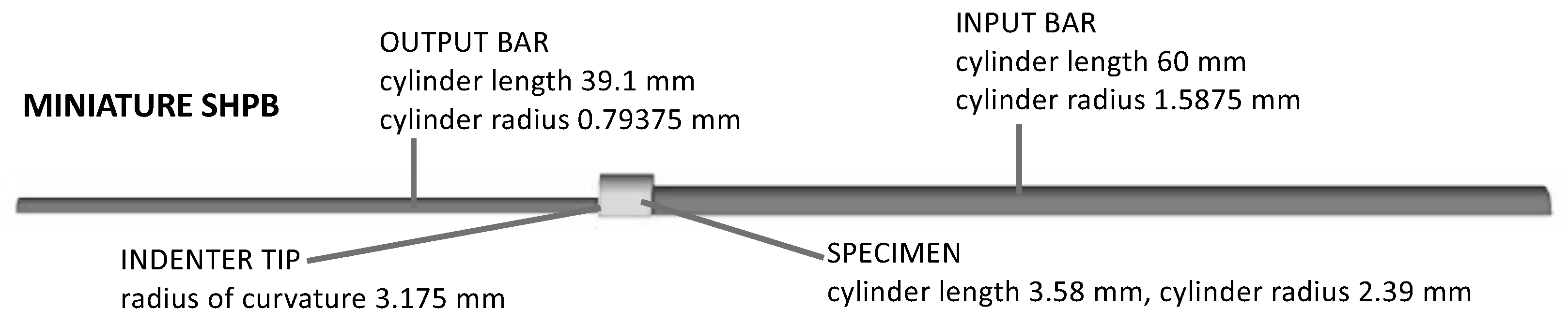
5.1. Experimental Protocols

Data from three dynamic spherical indentation experiments are analyzed using the equations and techniques of Section 2, Section 3 and Section 4. Experimental methods have been discussed by Casem [88,119] and are summarized in what follows.

A miniature Kolsky bar (i.e., SHPB) [120] is adapted for instrumented indentation, whereby transient force, displacement, and velocity data are acquired in each experiment. The loading history (e.g., indenter’s velocity) depends on the velocity of the striker bar and geometric properties of the system (including pulse shaping), as well as indentation resistance afforded by the substrate. Initial clearance between indenter and substrate also affects the velocity history. The loading history is thus not strictly controlled; however, different final indentation depths are generally achieved by increasing the striker velocity, commensurate with an increase in the average loading rate. Experimental data include both the loading and unloading histories for each test.

Relevant properties and parameters are listed in

Table 1. Material and geometric parameters.

Parameter (Units)	Value	Definition	Source
E (GPa)	71.0	modulus of Al 6061-T6	Wu et al. [121]
$\nu$ (-)	0.33	Poisson’s ratio of Al 6061-T6	Wu et al. [121]
${\rho }_0$ (g/cm${}^3$)	2.77	mass density of Al 6061-T6	Wu et al. [121]
$c_V$ (J/kg·K)	896	specific heat of Al 6061-T6	Zhu et al. [122]
${\sigma }_0$ (GPa)	0.25	initial yield strength of Al 6061-T6	Lesuer et al. [123], Zhu et al. [122]
$\kappa$ (-)	0.35–1.8	hardening coefficient range of Al 6061-T6	Lesuer et al. [123], Zhu et al. [122]
n (-)	0.38–0.43	hardening exponent range of Al 6061-T6	Lesuer et al. [123], Zhu et al. [122]
C (-) $[\simeq m]$	0.002–0.083	rate sensitivity range of Al 6061-T6	Lesuer et al. [123], Zhu et al. [122], Casem et al. [120]
q (-) $[\simeq -r]$	1.34	thermal softening of Al 6061-T6	Lesuer et al. [123]
${\dot{ϵ}}_0$ (1/s)	1.0	reference strain rate (universal)	Zhu et al. [122]
$T_M$ (K)	925	melt temperature of Al 6061-T6	Zhu et al. [122]
$T_R$ (K)	294	reference temperature (ambient)	Zhu et al. [122]
$\overline{E}$ (GPa)	71.2	system modulus with WC indenter	Weaver et al. [1]
R (mm)	3.175	indenter radius	this work

with supporting references. Of these values, those comprising the set of six strain-hardening, strain-rate, and temperature-sensitivity parameters $\{\kappa ,n;C$ or $m;q$ or $r;T_R,T_M\}$ are not used explicitly in the forthcoming analysis but are included for context to aid in interpretation of results. All current experiments are performed at standard room temperature: $T_0=T_R$. Prominent results are summarized in

Table 2. Loading conditions and results at max depth ${(·)}_m$ or averaged over the loading phase ${(·)}_A$.

Experiment	$\overline{\mathit{\upsilon }}$ (m/s)	${\mathit{h}}_{\mathit{m}}$ ($\mathsf{\mu }$m)	${\mathit{a}}_{\mathit{m}}$ ($\mathsf{\mu }$m)	${\mathit{W}}_{\mathit{m}}^{\mathit{P}}$ (mJ)	$\mathbf{\Delta }{\overline{\mathit{T}}}_{\mathit{m}}$ (K)	${\overline{\mathit{ϵ}}}_{\mathit{m}}$	${\widehat{\mathit{ϵ}}}_{\mathit{m}}$	${\dot{\overline{\mathit{ϵ}}}}_{\mathit{A}}$ (1/s)	${\dot{\widehat{\mathit{ϵ}}}}_{\mathit{A}}$ (1/s)	${\dot{\mathit{h}}}_{\mathit{A}}$ (m/s)
1	0.61	17.2	421	1.57	1.15	0.0265	0.0174	1386	908	0.90
2	1.06	25.0	508	3.82	1.59	0.0320	0.0209	2217	1452	1.74
3	1.36	35.7	606	8.43	2.06	0.0382	0.0250	2750	1801	2.57

for reference and are defined and discussed in detail later. Pertaining to loading conditions, $h_m$ in the leftmost column is the maximum indentation depth prior to unloading, and ${\dot{h}}_A$ in the rightmost column is the average indenter tip velocity over the loading phase of each experiment.

The substrate material is presumed to be isotropic, both elastically and plastically. Characterization and static indentation experiments on the same as-received Al 6061-T6 [1] suggest that, given the presently sized indenter, the volume of material sampled underneath the indenter at initial yield should contain 40 to 50 crystals of random orientation. Results by Weaver et al. [1] confirm that this is a sufficient number to ensure a repeatable, globally isotropic response. It is assumed here that isotropy carries over to the dynamic regime; similar indentation stress-strain curves presented later among multiple dynamic indentation experiments support this assumption, at least post yielding.

The miniature SHPB system equipped for indentation testing is sketched in Figure 1. This image only shows the upper half of the system, which is axially symmetric. The indenter is tungsten carbide (WC) with a radius $R=R_i$ of 3.175 mm. The spherical tip of the indenter is machined directly into the input bar, on its right side in Figure 1. The substrate is the aluminum alloy Al 6061-T6 of cylindrical geometry, with $L_s/D_s=\frac{3}{4}$ and $D_s=\frac{3}{2}{R}_i=\frac{3}{2}R$.

The velocity history $\upsilon \left(t\right)$ at the right side of the input bar in Figure 1 is acquired from analysis of transient data from a strain gauge. The average of this input velocity over the duration of each test is denoted by $\overline{\upsilon }$. As shown in Table 2, $\overline{\upsilon }$ increases with test number, as do all other observed or extracted quantities such as maximum depth, maximum indentation strains, and average indentation strain rates. In many subsequent figures, $\overline{\upsilon }$ is thus used to further distinguish experiments 1, 2, and 3. A normal displacement interferometer (NDI) focused at each of the indented faces of the sample at its radial edge (left end) and the left end of the output bar records displacement history for each location. Force and displacement histories for the tip of the indenter are computed from a linear elastic wave analysis with the strain gauge data and the NDI data.

Static spherical indentation experiments on this material have been reported elsewhere [38], albeit with an indenter of larger radius $2R$. Numerical simulations of the static problem [38] loaded to comparable indentation strain levels suggest that the current dimensions of the substrate are sufficiently large to mitigate boundary edge effects. However, the effects of stress wave interactions with finite boundaries cannot be ruled out in dynamic experiments.

The elastic stiffness of WC ($E_i=640$ GPa) is an order of magnitude larger than that of aluminum, and $\overline{E}$ in Table 1 accounts for the true elastic modulus of both the indenter and substrate, assumed to be known a priori. If a rigid indenter is assumed instead, then $\overline{E}$ increases by ≈10%. However, since the indenter material is held fixed among experiments, elastic properties of the indenter can be excluded from the list of independent variables in the forthcoming dimensional analysis, as assumed in the general framework of Section 4.

Indentation depth and tip velocity (i.e., depth rate) are inferred with respect to the far-field displacement of the surface of the sample and correctly account for rigid body motion. The reported indentation depth and depth rate are the respective true indentation depth $h_s$ and depth rate ${\dot{h}}_s$ in the substrate, relative to those measured for the far-field surface away from any pile-up or sink-in effects. In the remainder of Section 5, notation is simplified such that $h_s\to h$ and ${\dot{h}}_s\to \dot{h}$. Cursory calculations with the approximation in (3) confirm that the contribution of deformation of the spherical end of the indenter, $h_i$, to h should be negligible for loads and contact radii reported in what follows. Summarizing, the indenter can be considered rigid for purposes of setting $h=h_s$ and $R_i=$ constant, but it should have a finite modulus $E_i$ for accurately quantifying $\overline{E}$.

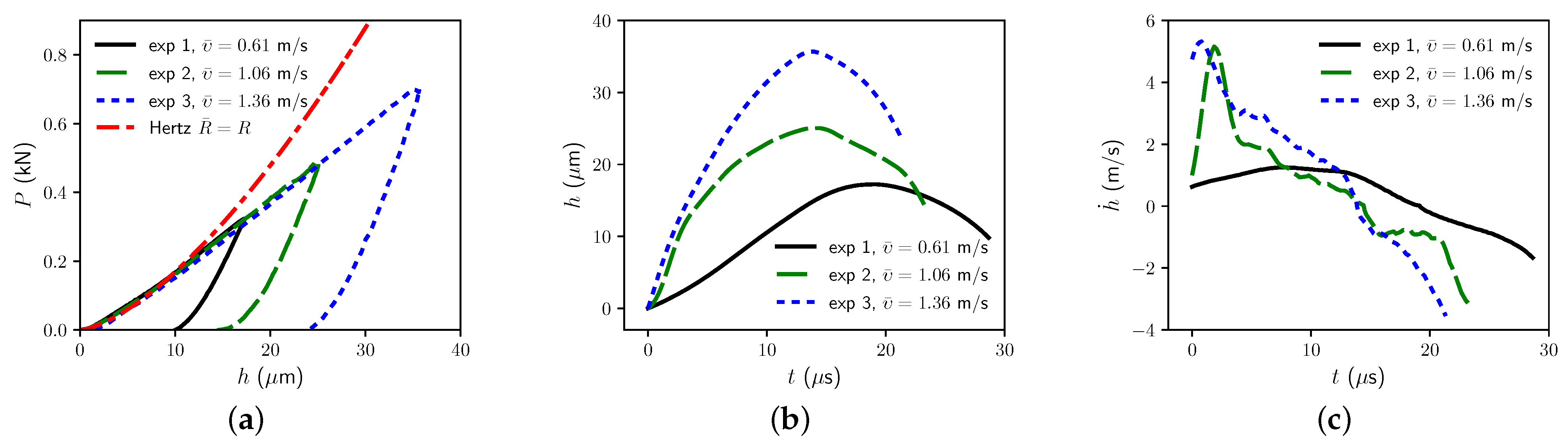
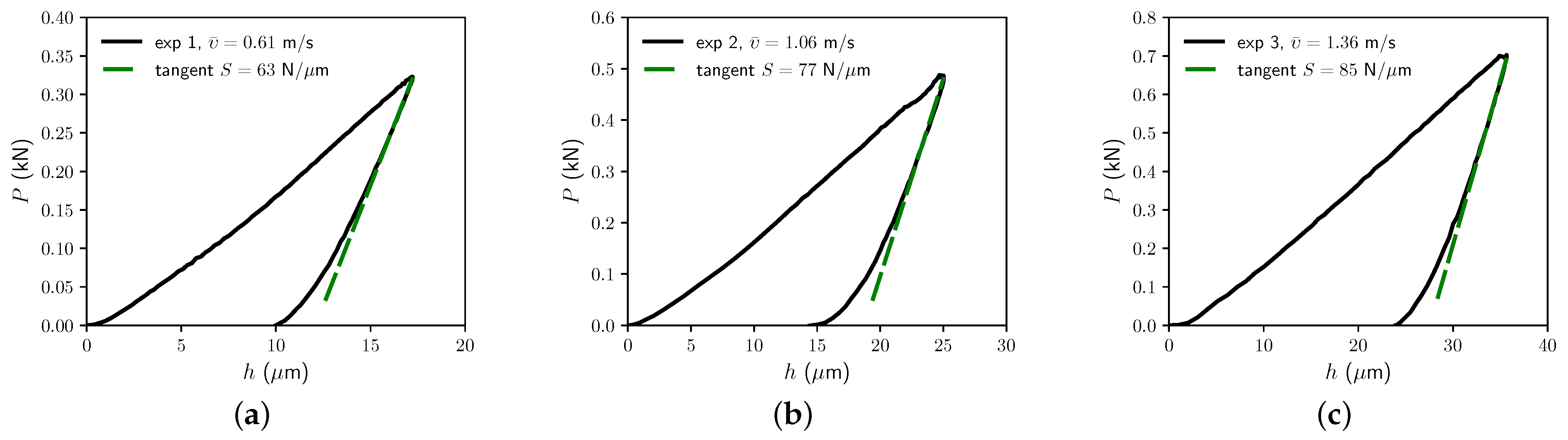
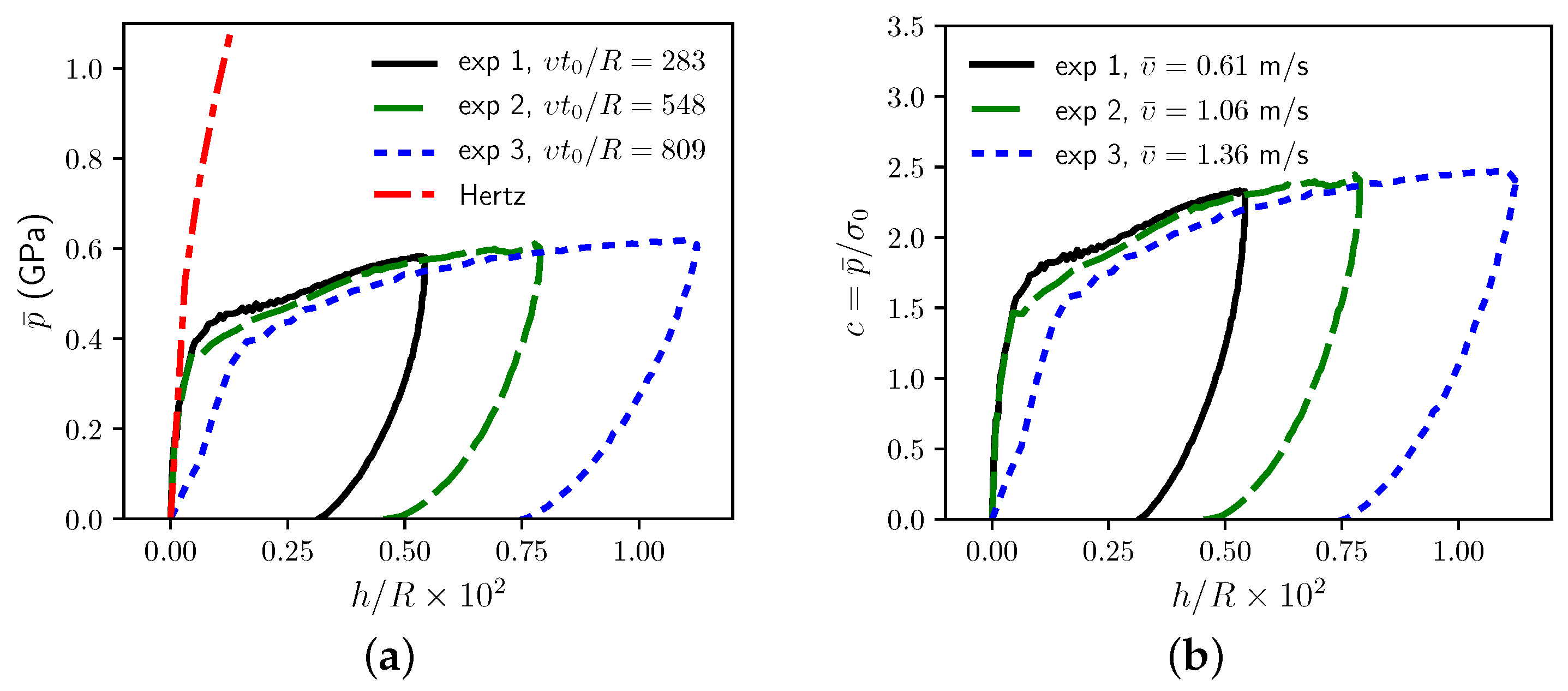
5.2. Data Analysis: Global Response

Experimental force–depth, depth–time, and depth rate–time histories are shown in Figure 2, labeled “exp” (for experiment) 1, 2, and 3. The time t at a given depth h is confirmed by the integral $t=\int (h/\dot{h})\mathrm{d}h$, where $\dot{h}$ is known as a function of h and initially $t=0$. Shown for reference in Figure 2a is the Hertz elastic solution of (1) obtained assuming $\overline{R}=R$ in (2).

For $h\gtrsim 10\mathsf{\mu }$m, the data are more compliant than the elastic solution, as expected for an elastic–plastic material post yielding. For $h\lesssim 10\mathsf{\mu }$m, experiments are similar to the elastic solution. Notably, some data appear slightly stiffer than the elastic solution over small intervals of h. These unusual features could be due to inertial effects and/or imprecision of experimental measurements at very low indentation depths. Depth–time histories shown in Figure 2b indicate total load–unload durations ranging from around 20 to 30 $\mathsf{\mu }$s. Maximum depth and depth rate increase with experiment number. Velocity histories are drastically different among experiments. For example, velocity ramps up quickly with time for experiment 2, while it is initially near maximal for experiment 3. In the latter case, the indenter clearly accelerates prior to contact with the substrate. Note $\dot{h}<0$ during the unloading phase of each experiment. Peak loading and unloading velocities are notably smaller for experiment 1 than experiments 2 and 3.

Force–depth data are delineated for each experiment in Figure 3, wherein the slope S upon initial unloading is extracted from the tangent for each case. The maximum indentation depth is denoted by $h_m$. The unloading slope S at $h=h_m$ is then used to obtain the Hertz contact radius at maximum depth $a_m=a(h=h_m)$, assuming quasi-static elastic unloading, via (5) [37,38]. Elastic modulus $\overline{E}$ is assumed, a priori, to have the value listed in Table 1. No attempt is made to extract elastic properties from the present indentation data, as has been performed in some investigations elsewhere [6].

Dimensionless dependent variables ($\mathsf{\Pi }$-terms) introduced in the analysis of Section 4 are reported in Figure 4. General functional forms are (25)–(27). In each figure, the independent variable resolved on the abscissa is dimensionless depth $h/R$ (or $h_m/R$), which is well-defined and fully known from the test data. Among different experiments, the normalized indentation velocity $\upsilon t_0/R$ also varies, as does the maximum normalized depth $h_m/R$. Since the substrate material and initial temperature (room temperature) are identical among experiments, the other independent variables on the right sides of (25)–(27) are fixed among the present results. Hence, potential influences of the latter (fixed) properties cannot be fully discerned or quantified among the presently available data. However, qualitative deductions on yielding, strain hardening, and rate sensitivity are still possible, as will be discussed later in the context of indentation stress–strain curves. A candidate definition for effective velocity is the average loading rate $\upsilon ={\dot{h}}_A=h_m/t_m$, where $t_m$ is the time instant at which $h=h_m$. As shown in the rightmost column of Table 2, ${\upsilon }_A$ increases from approximately 0.9 to 1.7 to 2.6 m/s over respective experiment numbers 1 to 2 to 3.

Normalized force ${\mathsf{\Pi }}_P$ versus normalized depth $h/R$ in Figure 4a provides the same information as in Figure 2a, since E and R are identical among experiments. Assuming $\upsilon ={\dot{h}}_A$, the results in Figure 4a show that the dependence of dimensionless indentation force ${\mathsf{\Pi }}_P$ on dimensionless loading rate $\upsilon t_0/R$ is low for Al 6061-T6 over the current domain of loading rates.

Since the present data do not contain intermittent unload–reload cycles or continuous stiffness measurements (CSM) to obtain unloading slope $S\left(h\right)$ for $h\ne h_m$, approximations are used to compute contact radius $a\left(h\right)$ for $h\ne h_m$. First, for the loading phase, $t\le t_m$, it is assumed that $a\left(t\right)$ for each experiment depends only on $h/R$ and not $\upsilon$. As shown in Figure 4b, the normalized radius ${\mathsf{\Pi }}_a$ is then estimated by the following function, where $\alpha \ge 0$ and $\beta \gg 1$ are dimensionless fitting constants:

$${\mathsf{\Pi }}_a=a/R=(1+\alpha \{1-\exp (-\beta h/R)\})\sqrt{h/R}[t\le t_m].$$

(33)

The Hertz solution is recovered in the limit of infinitesimal depth, whereby $a\to \sqrt{hR}$.

Available data do not enable fitting of $a\left(t\right)$ for $t>t_m$, i.e., throughout the entire unloading process. Thus, during unloading, it is assumed that the indentation stress–strain data (specifically, $\widehat{\sigma }=\overline{p}$ versus $\widehat{ϵ}$) demonstrate a fixed slope of $\overline{E}$, consistent with quasi-static unloading [5,26]. To this end, the following quadratic equation is solved at each time increment for $a\left(h\right(t\left)\right)$ during the unloading phase:

$$\frac{4\overline{E}}{3\pi }\left(\frac{h}{a}-\frac{h_r}{a_f}\right)=\frac{P}{\pi a^2}[t\ge t_m].$$

(34)

Here, $h_r$ is the final (residual) indentation depth upon complete unloading, and $a_f$ is the projected (not measured) final contact radius. The latter, which generally can differ from the observed residual imprint radius $a_r$, can be computed by solving (34) at $h=h_m$, with corresponding peak load $P=P_m$ measured and radius $a=a_m$ obtained from (33).

Finally, normalized plastic work ${\mathsf{\Pi }}_W$ is shown in Figure 4c. Its computation requires the entire load–unload force–displacement cycle for a given $h_m$; hence, only three data points are available (one for each experiment). Though not shown in Figure 4c, ${\mathsf{\Pi }}_W$ logically could depend on $h_r/R$ as well, since $h_r$ varies among experiments, increasing from 9.8 to 14.4 to 23.6 $\mathsf{\mu }$m over experiments 1, 2, and 3. Such dependency is permissible via inclusion of $h/R$ in addition to $h_m/R$ in the listed arguments of (27). However, the identity ${\mathsf{\Pi }}_P(h=h_r)=0$ provides an additional constraint equation that can be used to eliminate explicit dependence of ${\mathsf{\Pi }}_W$ on $h_r/R$. Normalized plastic work clearly increases with increasing maximum penetration depth.

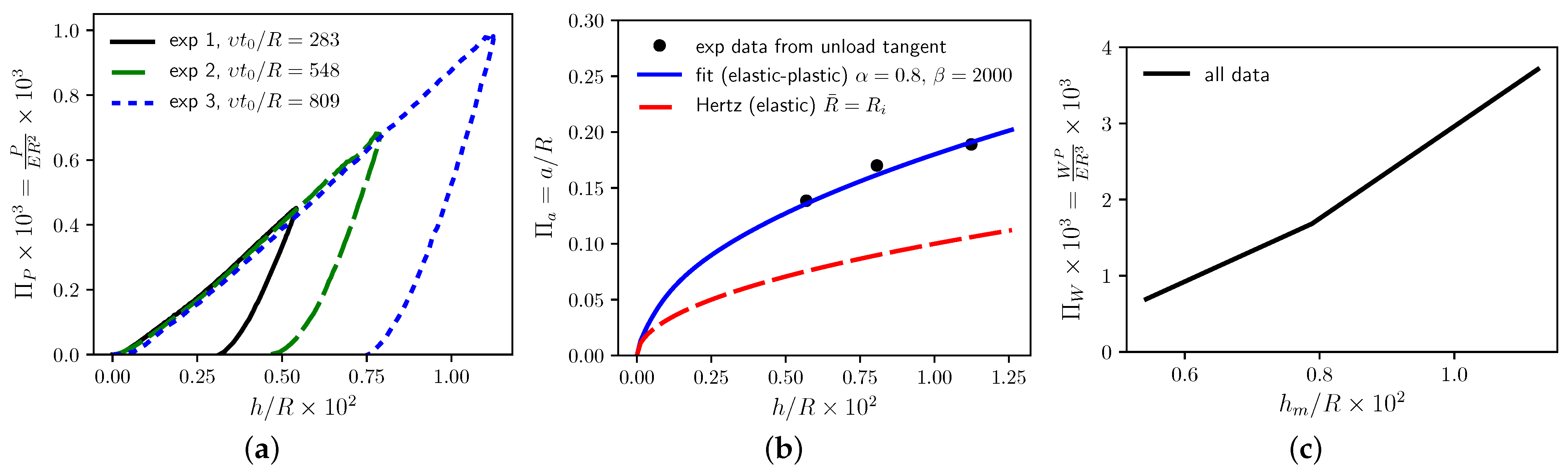
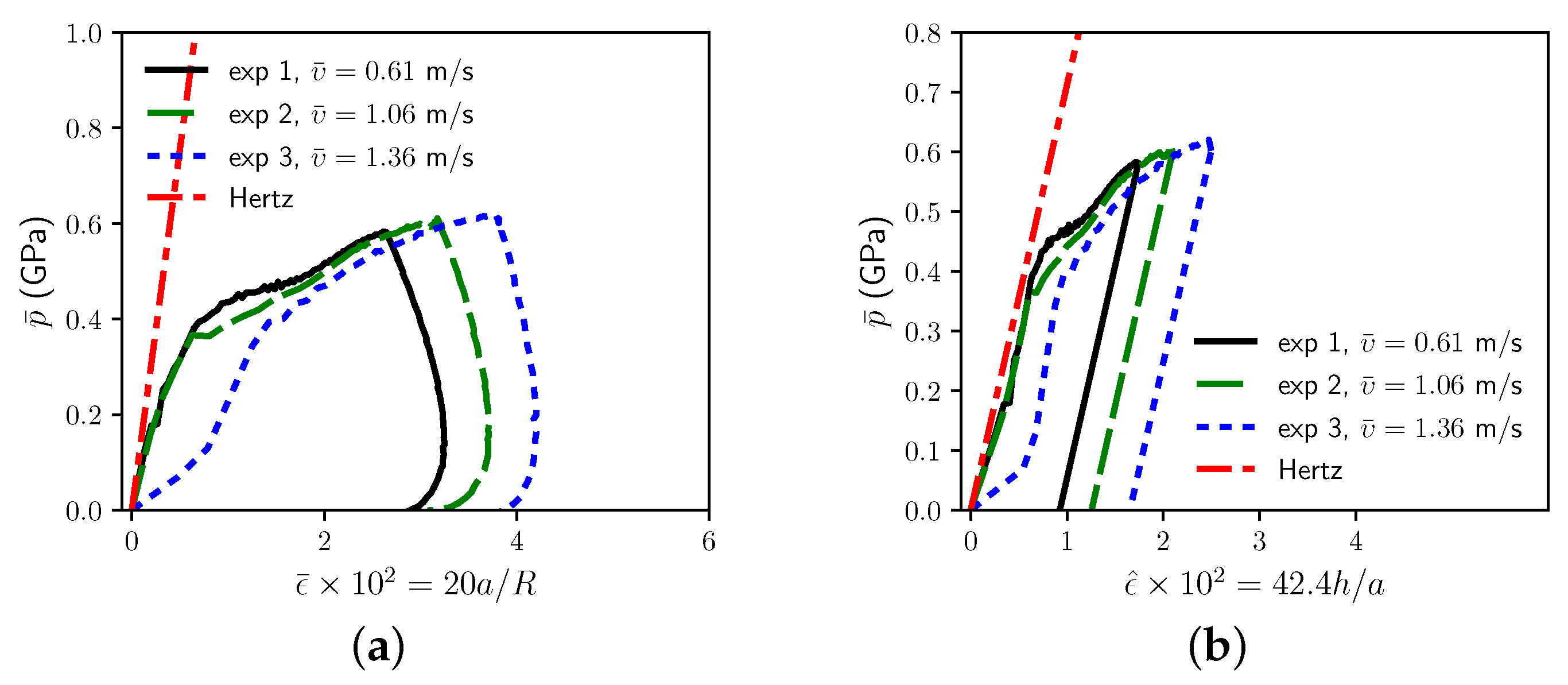
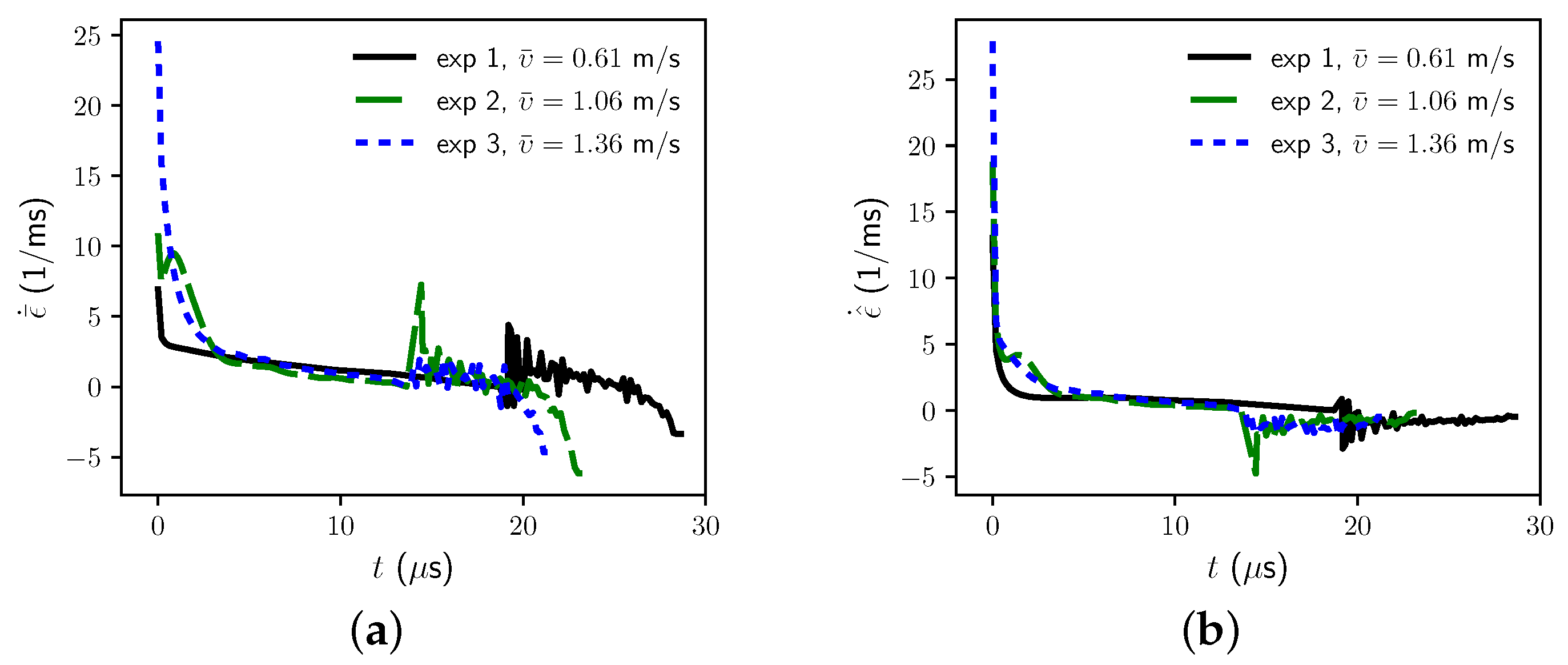
5.3. Data Analysis: Indentation Stress–Strain and Other Extracted Information

Typically, the global force–depth response is of primary interest from indentation testing, along with possible information on the contact radius. In the dynamic case, complete data should include time histories of these quantities. From such data, supplemental quantities such as indentation stress, indentation strain, indentation strain rate, and mean temperature rise can be computed, as demonstrated next. The reader interested only in the primary response (e.g., indentation force versus depth) emphasized in Section 5.2 can bypass the remainder of Section 5.3.

Given a (or equivalently, ${\mathsf{\Pi }}_a$), along with force data $P\left(h\right)$, mean pressure $\overline{p}=P/\left(\pi a^2\right)$ (e.g., Meyer’s hardness H when P is maximum and a is the residual imprint radius) is computed. Results are shown in Figure 5a. Constraint factor c is shown in Figure 5b, recalling that the initial yield stress ${\sigma }_0$ from Table 1 is used for normalization in Section 5. Note that this value of ${\sigma }_0$ is considered to be known a priori, rather than extracted from the present indentation data. Mean pressure closely tracks the Hertz solution at a very small $h/R$ for experiments 1 and 2, whereas $\overline{p}$ for experiment 3 suggests anomalously low compliance in the limit $h/R\to 0$. As displayed here in Figure 5 and Figure 6, the Hertz solution invokes the usual assumption $R_s\to \infty$ in (2). Mean pressures are similar among the loading phases of all three experiments for $h/R\gtrsim 0.0025$, in the regime where plastic compliance is expected to overtake elastic compliance. Such similarities suggest strain rate and strain rate–history effects on $\overline{p}$ are small for these experiments on Al 6061-T6, given the very different velocity histories among tests in Figure 2c.

Taking $\upsilon ={\dot{h}}_A$, the results in Figure 5a imply that dependence of mean stress on dimensionless loading rate $\upsilon t_0/R$ is low. In fact, the mean stress and constraint factor appear to decrease slightly with increasing loading rate, though such decrease may be due to imprecision of the experimental measurements and uncertainty inherent in (33) that neglects possible rate dependence of the transient contact radius.

Recall from the review in Section 2.2 that initial yielding corresponds to $c\approx 1.1$ in the quasi-static Hertz theory [6]. After yielding, the calculated constraint factor increases from $c\approx 1.5$ to $c\approx 2.5$ over the full domain of indentation depths in the experiments. Strain hardening likely influences c to increase with increasing $h/R$ in the fully plastic regime. The computed range of c is within bounds observed elsewhere in quasi-static spherical indentation experiments and simulations [1,2,6,37,42,43,44,45]. Similar ranges have been observed in dynamic spherical indentation simulations of elastic–perfectly plastic, rate-independent solids for constant rigid indenter velocities that are not too large (e.g., $\dot{h}\lesssim 75$ m/s), albeit for representative metallic substrates with different properties than those of aluminum [46]. Transient increases in c due to inertial effects manifest at velocities on the order of 100 m/s [46]; at such high velocities, the effects of strain rate sensitivity on c also become stronger [23]. During elastic unloading, c is easily computed given P and the current method of estimation of a, but its value does not have any physical significance.

Indentation stress (i.e., mean pressure $\overline{p}$) is reported versus the two different indentation strain measures of (32) in Figure 6. Elastic deformation followed by plastic yielding and mild-to-moderate strain hardening is apparent in each representation. The hardening behavior is qualitatively consistent with the traditional dynamic uniaxial stress–strain behavior of this material [120,122]. The anomalously high initial compliance of experiment 3 is also apparent in Figure 6. Elastic unloading is perfectly represented in Figure 6b, as a result of the implementation of (34). On the other hand, the unloading portions of $\overline{p}$ versus $\overline{ϵ}$ curves in Figure 6a show slopes inconsistent with $\overline{E}$. Similar inconsistencies have been noted when $\overline{ϵ}$ is used as the indentation strain measure for static indentation [5,26]. In Figure 6b, yielding is apparent at $\widehat{ϵ}\approx 0.6\%$ for experiments 1 and 2. From (13), with $c\approx 2.5$, the uniaxial-equivalent yield strain is then estimated as ${\sigma }_0/E\approx 0.25\%$.

Strain rates in (19) and (22) are consistently obtained from numerical differentiation of (32). Results are shown in Figure 7. According to each strain definition, strain rates are initially large over domains wherein both the indentation depth and contact radius increase rapidly with time. Initial values of $\dot{\overline{ϵ}}$ and $\dot{\widehat{ϵ}}$ range from 7000/s to 28,000/s, with the highest strain rates observed in experiment 3. Strain rates decrease subsequently with increasing time, as the indenter necessarily decelerates. Negative rates persist during unloading. However, oscillations also arise during unloading to accommodate the assumed form of contact radius in the elastic response function of (34).

Due to uncertainty in assumed relations (33) and (34), the strain-rate histories shown in Figure 7 should be considered highly approximate. However, average strain rates during the loading phase of each test should be much more accurate, since these do not rely on (33) or (34). Rather, such averages depend only on the unloading slope S in (5) used to obtain $a_m=\frac{1}{2}S/\overline{E}$ at known time $t_m$ at the measured depth $h=h_m$:

$${\dot{\overline{ϵ}}}_A=0.2\frac{a_m}{R{t}_m},{\dot{\widehat{ϵ}}}_A=\frac{4}{3\pi }\frac{h_m}{a_m{t}_m}.$$

(35)

Values of these average strain rates are listed in Table 2. Notably, average rates follow the same trends over all three experiments, with ${\dot{\overline{ϵ}}}_A\approx 1.5{\dot{\widehat{ϵ}}}_A$ in each case. These average strain rates are within ranges that can be obtained in conventional uniaxial SHPB experiments on this material [122,123].

The same trends apply for maximum strains: ${\overline{ϵ}}_m\approx 1.5{\widehat{ϵ}}_m$ in all three experiments. Values of ${\widehat{ϵ}}_m$ range from 1.8% to 2.5%. Taking $\widehat{\beta }\approx 1.3$ in (13), as in earlier simulations of other elastic–plastic materials [37], maximum uniaxial-equivalent strains are then approximated as ranging from 1.4% to 1.9%.

Applying a representative rate sensitivity parameter of $C=0.01$ from Table 1, the ratio of dynamic flow stress at a strain rate of 2000/s is predicted by the Johnson–Cook model to be only 7.6% higher than that at a rate of 1000/s. Accordingly, any effects of different strain rates witnessed in experiments 1, 2, and 3 may be too small to be discerned in the load–displacement or indentation stress–strain curves. Viewed differently, the relatively low strain-rate sensitivity of the Al 6061-T6 material is corroborated by the similar indentation stress–strain curves among experiments at different transient and average loading rates. However, mild rate sensitivity effects, if they exist, might also be obscured by limited fidelity and the limited strain-rate range of the data.

Other discrete data of interest are included in Table 2. Maximum depth $h_m$ and corresponding contact radius $a_m$ were discussed already in the context of Figure 4a,b. Average velocities ${\dot{h}}_A$ are used to represent $\upsilon$ entering dimensionless rates in the legends of Figure 4a and Figure 5a. Likewise, plastic work $W_m^P$ is used in the construction of Figure 4c. Note that $W_m^P$ is the residual plastic work after complete unloading from depth $h_m$.

The average adiabatic temperature rise at maximum depth, $\Delta {\overline{T}}_m$, is computed from the second of (31), with $W^P=W_m^P$ and $a=a_m$. This is the temperature change that would be experienced by a cylindrical column of plastically deformed material of radius $a_m$ and height $\frac{3}{4}\pi a_m$ [5,26]. Given the temperature sensitivity $q\approx 1$ of Al 6061-T6 in Table 1, the predicted heating-induced change in flow stress (i.e., thermal softening) for this volume of material should be negligible. However, localized temperature increases in regions of concentrated plastic strain (e.g., near the edges of the contact surface) could be substantially larger, whereas heat conduction could counteract such increases given sufficient time. Thus, thermal effects cannot be completely ruled out without verification from simulations, for example.

5.4. Summary and Recommendations

The following key points are ascertained from analysis of the dynamic indentation data:

• Maximum uniaxial-equivalent strains are estimated from maximum indentation strains to be on the order of 1% to 2%;
• Average uniaxial-equivalent strain rates are estimated from indentation strain rates to be on the order of 700 to 1500/s;
• Subtle variations in indentation force–depth curves can lead to drastic changes in indentation stress–strain curves, particularly at small indentation depths;
• Dynamic indentation stress–strain curves are qualitatively similar to those given elsewhere [37,38] for static spherical indentation, with constraint factors within ranges observed for static experiments on ductile metals;
• Mean pressure (i.e., indentation stress) shows evidence of yielding and mild-to-moderate strain-hardening characteristic in uniaxial stress–strain data for the aluminum alloy 6061-T6;
• Strain rate and inertial effects are not detected among the experimental datasets, whereby an increase in average indentation strain rate by a factor of 2 produces no apparent increase in indentation stress;
• A negligible effect of average strain rate correlates with the low strain-rate sensitivity of flow stress for the aluminum alloy, as measured in traditional SHPB experiments;
• Plastic work results in a trivially small adiabatic temperature rise ($\lesssim$2K) averaged over the entire plastically deformed zone, though magnitudes of localized temperature increases at plastic strain concentrations are unknown.

Consider the inverse problem of determination of material parameters (elastic, thermo-mechanical, and plastic entering (14) and (16)) from recorded indentation force versus depth, i.e., $P=E{R}^2·{\mathsf{\Pi }}_P$ versus h, data for different loading velocities (e.g., average indentation depth rates) $\upsilon$ and ambient temperatures $T_0$. In this context, R is known a priori, $T_0$ and $\upsilon$ are imposed, P and h are measured, and E is presumably unknown and thus to be determined.

It may not be possible to determine E given only dimensionless ${\mathsf{\Pi }}_P$ versus $h/R$ data. For example, for purely elastic Hertz-type indentation, the dimensionless force–displacement response of (28) is independent of E. Therefore, at least some experimental data should be recorded in dimensional, rather than dimensionless, form to allow for determination of all of the normalization constants of the dimensional analysis: $R,E,t_0,\tilde{T}$. In other words, measurement of P rather than ${\mathsf{\Pi }}_P$ reintroduces a stress scale into the inverse problem, in principle enabling implicit extraction of E. Similarly, measurement or knowledge of R reintroduces an independent length scale into the problem. Measurement or imposition of $\upsilon$ rather than $\frac{\upsilon t_0}{R}$ reintroduces an independent time scale (i.e., $\frac{R}{\upsilon }$ given R), and measurement or imposition of $T_0$ rather than $\frac{\tilde{T}}{T_0}$ reintroduces an independent temperature scale.

The inverse problem can be stated as follows:

• Given $\frac{P}{R^2}=E·{\mathsf{\Pi }}_P\left(\frac{h}{R},\frac{\upsilon t_0}{R},\frac{\tilde{T}}{T_0};\frac{{\sigma }_0}{E},\frac{R/t_0}{\sqrt{E/{\rho }_0}},\frac{\tilde{T}}{T_R},\nu ,\kappa ,m,n,r\right)$ versus $\frac{h}{R}$ for different effective loading strain rates $\upsilon /R$ and initial temperatures $T_0$, determine the eleven material properties $E,\nu ,{\rho }_0,c_V,{\sigma }_0,\kappa ,{\dot{ϵ}}_0=t_0^{-1},m,n,r,T_R$. (The list of sought properties is reduced to nine if ${\dot{ϵ}}_0$ and $T_R$ are regarded as fixed universal constants.)

In the present dynamic indentation experiments, the dimensionless response function ${\mathsf{\Pi }}_a$ for contact radius cannot be precisely measured at present over the entire deformation history, and response function $E{R}^3·{\mathsf{\Pi }}_W$ ultimately offers no additional information over $E{R}^2·{\mathsf{\Pi }}_P$, since the former can be constructed from the history of the latter. Based on dimensional analysis of available results, the following deductions and recommendations are then proposed to facilitate the solution of the inverse problem:

• The relatively small magnitudes of impact velocities and the similarities of static and dynamic indentation curves suggest that inertial effects associated with ${\rho }_0$ cannot be discerned in the data. Thus, a standard (e.g., Archimedes) method should be used to measure ${\rho }_0$.
• The relatively low changes in average temperature suggest that effects of specific heat capacity $c_V$ cannot be easily discerned in the force response data. Thus, a standard (e.g., calorimetry) method should be used to measure $c_V$.
• Precision of current experimental methods in the very small-depth regime is likely insufficient to directly ascertain elastic compliance via comparison with Hertz’s solution. Elastic (shallow) force–depth data also seem unable to delineate E and $\nu$ distinctly, since P depends only on $E/(1-{\nu }^2)$ and not E and $\nu$ independently in the Hertz solution. Thus, a standard (e.g., longitudinal and shear wave speed) method should be used to measure E and $\nu$. Any experimental facility equipped for dynamic instrumented indentation should include the capability for such sound speed measurements, presuming material samples are available.
• The precision of current experimental methods is likely inadequate for determination of an “exact” initial yield stress ${\sigma }_0$. However, an offset yield stress should be measurable, which can provide an approximate value of ${\sigma }_0$ as in static experiments [37].
• For low loading rates or rate-insensitive materials, extraction of static hardening parameters $\kappa$ and n should be possible from measured increases of ${\mathsf{\Pi }}_P$ with increasing $h/R$, though unique determination of both parameters may or may not be difficult.
• Effects of loading rate $\upsilon t_0/R$ on ${\mathsf{\Pi }}_P$ for highly rate-sensitive materials remains unknown. Experiments on other solids with much greater strain-rate sensitivity of flow stress are needed to determine if such rate sensitivity manifests in dynamic indentation force–displacement (and corresponding indentation stress–strain) curves over comparable domains of average indentation strain rates. If differences in ${\mathsf{\Pi }}_P$ at vastly different $\upsilon t_0/R$ do not manifest for such materials, the present experimental method might be unsuitable to extract rate sensitivity parameters (e.g., m, or C if (15) is used).
• Following typical protocols [93,122], the two parameters ${\dot{ϵ}}_0$ and $T_R$ can be set universally at 1/s and 294 or 300 K, which reduces the complexity of the inverse problem, as noted already.
• Presumably, systematic matching of experimental $E{R}^2·{\mathsf{\Pi }}_P$ data with results of parametric FE simulations on the same geometry (sample size and R), loading rate history, and initial temperature, and covering a sufficient domain of possible material property sets, will produce the sought material property relationships. Similar efforts have been undertaken for static indentation, as reviewed in Section 2.3, though most not invoking dimensional analysis techniques.
• The existence, uniqueness, stability, and accuracy of the inverse method should be verified for multiple materials, with constitutive properties validated by comparison with values obtained from independent, alternative experimental techniques (e.g., standard SHPB compression tests rather than dynamic indentation).

Several other recommendations are in order. Firstly, experimental methods to directly measure the contact radius during dynamic indentation could supply data that would render the assumed rate-independent forms in (33) and (34) unnecessary. Efforts are presently underway to measure residual impressions with confocal microscopy. Techniques involving periodic dynamic unloading in the SHPB apparatus to measure contact stiffness are also under development [88], though their accuracy remains unclear.

While knowledge of $a={\mathsf{\Pi }}_A·R$ is not needed to solve the stated inverse problem, the contact radius is needed to calculate indentation stress (mean pressure) $\overline{p}$, as well as indentation strains $\overline{ϵ}$ and $\widehat{ϵ}$. Constitutive property extraction might be more efficient and accurate by matching experimental and simulated indentation stress–strain curves rather than matching $P=E{R}^2·{\mathsf{\Pi }}_P$ vs. h or $h/R$.

Comparison of static and dynamic isothermal FE simulations on the same geometry (i.e., same sample size and R), for a hypothetical rate-independent material, would enable verification of the tentative conclusion that inertial effects are negligible for the present range of loading rates. Lastly, adiabatic FE simulations could be used to provide an upper bound on localized temperature rise in highly strained regions under the indenter, and thus verify the tentative conclusion that effects of temperature rise (but not necessarily initial temperature) on indentation force are negligible over the present range of loading rates.

6. Conclusions

Static and dynamic indentation methods for ductile metals were reviewed. This review focused on spherical indentation, including experiments, analytical fundamentals, and numerical models; the motivation being extraction of information on the constitutive response of the indented material. Analytical foundations for the interpretation of data from instrumented dynamic spherical indentation experiments were established.

To demonstrate and extend concepts covered in the literature review, a framework to guide future experiments and numerical simulations was set forth based on principles of dimensional analysis. The ultimate intent is acquiring constitutive properties, here focused on plastic properties of ductile metals, from dynamic indentation force–depth data at different loading rates and different initial temperatures. In a representative application, the potential utility and limitations of this framework were assessed using data collected on Al 6061-T6, obtained from SHPB experiments equipped for instrumented spherical indentation. The analysis revealed that average strain rates achieved in experiments are on the order of ${10}^3$/s, with maximum equivalent strains on the order of 2%. Indentation stress–strain results verify that the strain-rate sensitivity of the alloy is low.

References

1. Weaver, J.; Khosravani, A.; Castillo, A.; Kalidindi, S. High throughput exploration of process-property linkages in Al-6061 using instrumented spherical microindentation and microstructurally graded samples. Integr. Mater. Manuf. Innov. 2016, 5, 192–211. [Google Scholar] [CrossRef] [Green Version]
2. Taljat, B.; Zacharia, T.; Kosel, F. New analytical procedure to determine stress-strain curve from spherical indentation data. Int. J. Solids Struct. 1998, 35, 4411–4426. [Google Scholar] [CrossRef]
3. Mesarovic, S.; Fleck, N. Spherical indentation of elastic–plastic solids. Proc. R. Soc. Lond. A 1999, 455, 2707–2728. [Google Scholar] [CrossRef]
4. Clayton, J. Spherical Indentation in Elastoplastic Materials: Modeling and Simulation; Technical Report ARL-TR-3516; US Army Research Laboratory, Aberdeen Proving Ground: Adelphi, MD, USA, 2005. [Google Scholar]
5. Pathak, S.; Kalidindi, S. Spherical nanoindentation stress–strain curves. Mater. Sci. Eng. R 2015, 91, 1–36. [Google Scholar] [CrossRef] [Green Version]
6. Field, J.; Swain, M. A simple predictive model for spherical indentation. J. Mater. Res. 1993, 8, 297–306. [Google Scholar] [CrossRef]
7. Cheng, Y.T.; Cheng, C.M. Scaling, dimensional analysis, and indentation measurements. Mater. Sci. Eng. R 2004, 44, 91–149. [Google Scholar] [CrossRef]
8. Barick, M.; Gaillard, Y.; Lejeune, A.; Amiot, F.; Richard, F. On the uniqueness of intrinsic viscoelastic properties of materials extracted from nanoindentation using FEMU. Int. J. Solids Struct. 2020, 202, 929–946. [Google Scholar] [CrossRef]
9. Chen, X.; Hutchinson, J.; Evans, A. The mechanics of indentation induced lateral cracking. J. Am. Ceram. Soc. 2005, 88, 1233–1238. [Google Scholar] [CrossRef]
10. Armstrong, R. On size effects in polycrystal plasticity. J. Mech. Phys. Solids 1961, 9, 196–199. [Google Scholar] [CrossRef]
11. Voyiadjis, G.; Yaghoobi, M. Review of nanoindentation size effect: Experiments and atomistic simulation. Crystals 2017, 7, 321. [Google Scholar] [CrossRef]
12. Voyiadjis, G.; Yaghoobi, M. Size Effects in Plasticity: From Macro to Nano; Academic Press: London, UK, 2019. [Google Scholar]
13. Armstrong, R. Dislocation mechanics pile-up and thermal activation roles in metal plasticity and fracturing. Metals 2019, 9, 154. [Google Scholar] [CrossRef] [Green Version]
14. Abu Al-Rub, R.; Voyiadjis, G. Analytical and experimental determination of the material intrinsic length scale of strain gradient plasticity theory from micro-and nano-indentation experiments. Int. J. Plast. 2004, 20, 1139–1182. [Google Scholar] [CrossRef]
15. Voyiadjis, G.; Song, Y. Strain gradient continuum plasticity theories: Theoretical, numerical and experimental investigations. Int. J. Plast. 2019, 121, 21–75. [Google Scholar] [CrossRef]
16. Zubelewicz, A. Mechanisms-based transitional viscoplasticity. Crystals 2020, 10, 212. [Google Scholar] [CrossRef] [Green Version]
17. Clayton, J.; Aydelotte, B.; Becker, R.; Hilton, C.; Knap, J. Continuum modelling and simulation of indentation in transparent single crystalline minerals and energetic solids. In Applied Nanoindentation in Advanced Materials; Tiwari, A., Ed.; Wiley: Hoboken, NJ, USA, 2017; Chapter 15; pp. 347–368. [Google Scholar]
18. Knap, J.; Ortiz, M. Effect of indenter-radius size on Au (001) nanoindentation. Phys. Rev. Lett. 2003, 90, 226102. [Google Scholar] [CrossRef] [PubMed] [Green Version]
19. Buckingham, E. On physically similar systems; illustrations of the use of dimensional equations. Phys. Rev. 1914, 4, 345–376. [Google Scholar] [CrossRef]
20. Sedov, L. Similarity and Dimensional Methods in Mechanics; Academic Press: London, UK, 1959. [Google Scholar]
21. Ni, W.; Cheng, Y.T.; Cheng, C.M.; Grummon, D. An energy-based method for analyzing instrumented spherical indentation experiments. J. Mater. Res. 2004, 19, 149–157. [Google Scholar] [CrossRef]
22. Clayton, J. Penetration resistance of armor ceramics: Dimensional analysis and property correlations. Int. J. Impact Eng. 2015, 85, 124–131. [Google Scholar] [CrossRef]
23. Lee, A.; Komvopoulos, K. Dynamic spherical indentation of strain hardening materials with and without strain rate dependent deformation behavior. Mech. Mater. 2019, 133, 128–137. [Google Scholar] [CrossRef]
24. Johnson, K. Contact Mechanics; Cambridge University Press: Cambridge, UK, 1985. [Google Scholar]
25. Ghaednia, H.; Wang, X.; Saha, S.; Xu, Y.; Sharma, A.; Jackson, R. A review of elastic–plastic contact mechanics. Appl. Mech. Rev. 2017, 69, 060804. [Google Scholar] [CrossRef]
26. Kalidindi, S.; Pathak, S. Determination of the effective zero-point and the extraction of spherical nanoindentation stress–strain curves. Acta Mater. 2008, 56, 3523–3532. [Google Scholar] [CrossRef]
27. Clayton, J.; Becker, R. Modeling Nonlinear Elastic-Plastic Behavior of RDX Single Crystals during Indentation; Technical Report ARL-TR-5864; US Army Research Laboratory, Aberdeen Proving Ground: Adelphi, MD, USA, 2005. [Google Scholar]
28. Oliver, W.; Pharr, G. An improved technique for determining hardness and elastic modulus using load and displacement sensing indentation experiments. J. Mater. Res. 1992, 7, 1564–1583. [Google Scholar] [CrossRef]
29. Dao, M.; Chollacoop, N.; Van Vliet, K.; Venkatesh, T.; Suresh, S. Computational modeling of the forward and reverse problems in instrumented sharp indentation. Acta Mater. 2001, 49, 3899–3918. [Google Scholar] [CrossRef] [Green Version]
30. Chollacoop, N.; Dao, M.; Suresh, S. Depth-sensing instrumented indentation with dual sharp indenters. Acta Mater. 2003, 51, 3713–3729. [Google Scholar] [CrossRef]
31. Cao, Y.P.; Lu, J. A new method to extract the plastic properties of metal materials from an instrumented spherical indentation loading curve. Acta Mater. 2004, 52, 4023–4032. [Google Scholar] [CrossRef]
32. Johnson, K. The correlation of indentation experiments. J. Mech. Phys. Solids 1970, 18, 115–126. [Google Scholar] [CrossRef]
33. Zhao, M.; Ogasawara, N.; Chiba, N.; Chen, X. A new approach to measure the elastic–plastic properties of bulk materials using spherical indentation. Acta Mater. 2006, 54, 23–32. [Google Scholar] [CrossRef]
34. Phadikar, J.; Bogetti, T.; Karlsson, A. Aspects of experimental errors and data reduction schemes from spherical indentation of isotropic materials. J. Eng. Mater. Technol. 2014, 136, 031005. [Google Scholar] [CrossRef]
35. Le, M.Q. Material characterization by instrumented spherical indentation. Mech. Mater. 2012, 46, 42–56. [Google Scholar] [CrossRef]
36. Donohue, B.; Ambrus, A.; Kalidindi, S. Critical evaluation of the indentation data analyses methods for the extraction of isotropic uniaxial mechanical properties using finite element models. Acta Mater. 2012, 60, 3943–3952. [Google Scholar] [CrossRef]
37. Patel, D.; Kalidindi, S. Correlation of spherical nanoindentation stress-strain curves to simple compression stress-strain curves for elastic-plastic isotropic materials using finite element models. Acta Mater. 2016, 112, 295–302. [Google Scholar] [CrossRef] [Green Version]
38. Fernandez-Zelaia, P.; Joseph, V.; Kalidindi, S.; Melkote, S. Estimating mechanical properties from spherical indentation using Bayesian approaches. Mater. Des. 2018, 147, 92–105. [Google Scholar] [CrossRef]
39. Lu, L.; Dao, M.; Kumar, P.; Ramamurty, U.; Karniadakis, G.; Suresh, S. Extraction of mechanical properties of materials through deep learning from instrumented indentation. Proc. Natl. Acad. Sci. USA 2020, 117, 7052–7062. [Google Scholar] [CrossRef] [PubMed] [Green Version]
40. Chen, G.; Zhang, X.; Zhong, J.; Shi, J.; Wang, Q.; Guan, K. New inverse method for determining uniaxial flow properties by spherical indentation test. Chin. J. Mech. Eng. 2021, 34, 94. [Google Scholar] [CrossRef]
41. Simo, J.; Hughes, T. Computational Inelasticity; Springer: New York, NY, USA, 1998. [Google Scholar]
42. Francis, H. Phenomenological analysis of plastic spherical indentation. J. Eng. Mater. Technol. 1976, 98, 272–281. [Google Scholar] [CrossRef]
43. Matthews, J. Indentation hardness and hot pressing. Acta Metall. 1980, 28, 311–318. [Google Scholar] [CrossRef]
44. Tabor, D. The Hardness of Metals; Oxford University Press: Oxford, UK, 1951. [Google Scholar]
45. Hill, R.; Storåkers, B.; Zdunek, A. A theoretical study of the Brinell hardness test. Proc. R. Soc. Lond. A 1989, 423, 301–330. [Google Scholar]
46. Lee, A.; Komvopoulos, K. Dynamic spherical indentation of elastic-plastic solids. Int. J. Solids Struct. 2018, 146, 180–191. [Google Scholar] [CrossRef]
47. Follansbee, P.; Sinclair, G. Quasi-static normal indentation of an elasto-plastic half-space by a rigid sphere–I: Analysis. Int. J. Solids Struct. 1984, 20, 81–91. [Google Scholar] [CrossRef]
48. Bhattacharya, A.; Nix, W. Finite element simulation of indentation experiments. Int. J. Solids Struct. 1988, 24, 881–891. [Google Scholar] [CrossRef]
49. Lee, H.; Lee, J.H.; Pharr, G. A numerical approach to spherical indentation techniques for material property evaluation. J. Mech. Phys. Solids 2005, 53, 2037–2069. [Google Scholar] [CrossRef]
50. Moussa, C.; Hernot, X.; Bartier, O.; Delattre, G.; Mauvoisin, G. Identification of the hardening law of materials with spherical indentation using the average representative strain for several penetration depths. Mater. Sci. Eng. A 2014, 606, 409–416. [Google Scholar] [CrossRef] [Green Version]
51. Moussa, C.; Hernot, X.; Bartier, O.; Delattre, G.; Mauvoisin, G. Evaluation of the tensile properties of a material through spherical indentation: Definition of an average representative strain and a confidence domain. J. Mater. Sci. 2014, 49, 592–603. [Google Scholar] [CrossRef] [Green Version]
52. Arizzi, F.; Rizzi, E. Elastoplastic parameter identification by simulation of static and dynamic indentation tests. Model. Simul. Mater. Sci. Eng. 2014, 22, 035017. [Google Scholar] [CrossRef]
53. Dean, J.; Clyne, T. Extraction of plasticity parameters from a single test using a spherical indenter and FEM modelling. Mech. Mater. 2017, 105, 112–122. [Google Scholar] [CrossRef]
54. Huber, N.; Tsakmakis, C. Determination of constitutive properties from spherical indentation data using neural networks. Part I: The case of pure kinematic hardening in plasticity laws. J. Mech. Phys. Solids 1999, 47, 1569–1588. [Google Scholar] [CrossRef]
55. Huber, N.; Tsakmakis, C. Determination of constitutive properties from spherical indentation data using neural networks. Part II: Plasticity with nonlinear isotropic and kinematic hardening. J. Mech. Phys. Solids 1999, 47, 1589–1607. [Google Scholar] [CrossRef]
56. Wang, M.; Wang, W. An inverse method for measuring elastoplastic properties of metallic materials using Bayesian model and residual imprint from spherical indentation. Materials 2021, 14, 7105. [Google Scholar] [CrossRef] [PubMed]
57. Cheng, Y.T.; Cheng, C.M. Relationships between hardness, elastic modulus, and the work of indentation. Appl. Phys. Lett. 1998, 73, 614–616. [Google Scholar] [CrossRef]
58. Cheng, Y.T.; Li, Z.; Cheng, C.M. Scaling relationships for indentation measurements. Philos. Mag. A 2002, 82, 1821–1829. [Google Scholar] [CrossRef]
59. Chen, X.; Ogasawara, N.; Zhao, M.; Chiba, N. On the uniqueness of measuring elastoplastic properties from indentation: The indistinguishable mystical materials. J. Mech. Phys. Solids 2007, 55, 1618–1660. [Google Scholar] [CrossRef]
60. Liu, L.; Ogasawara, N.; Chiba, N.; Chen, X. Can indentation technique measure unique elastoplastic properties. J. Mater. Res. 2009, 24, 784–800. [Google Scholar] [CrossRef]
61. Cao, Y.; Lu, J. Depth-sensing instrumented indentation with dual sharp indenters: Stability analysis and corresponding regularization schemes. Acta Mater. 2004, 52, 1143–1153. [Google Scholar] [CrossRef]
62. Barick, M. Identification of the Viscoelastic-Viscoplastic Properties of Materials by Instrumented Nanoindentation. Ph.D. Thesis, Université Bourgogne Franche-Comté, Besançon, France, 2020. [Google Scholar]
63. Clayton, J. Nonlinear Mechanics of Crystals; Springer: Dordrecht, The Netherlands, 2011. [Google Scholar]
64. Wu, J.; Wang, M.; Hui, Y.; Zhang, Z.; Fan, H. Identification of anisotropic plasticity properties of materials using spherical indentation imprint mapping. Mater. Sci. Eng. A 2018, 723, 269–278. [Google Scholar] [CrossRef]
65. Clayton, J.; Becker, R. Elastic-plastic behavior of cyclotrimethylene trinitramine single crystals under spherical indentation: Modeling and simulation. J. Appl. Phys. 2012, 111, 063512. [Google Scholar] [CrossRef]
66. Patel, D.; Al-Harbi, H.; Kalidindi, S. Extracting single-crystal elastic constants from polycrystalline samples using spherical nanoindentation and orientation measurements. Acta Mater. 2014, 79, 108–116. [Google Scholar] [CrossRef]
67. Choi, I.C.; Yoo, B.G.; Kim, Y.J.; Jang, J.I. Indentation creep revisited. J. Mater. Res. 2012, 27, 3–11. [Google Scholar] [CrossRef]
68. Yang, S.; Lu, W.; Ling, X. Spherical indentation creep characteristics and local deformation analysis of 310S stainless steel. Eng. Fail. Anal. 2020, 118, 104946. [Google Scholar] [CrossRef]
69. Ogbonna, N.; Fleck, N.; Cocks, A. Transient creep analysis of ball indentation. Int. J. Mech. Sci. 1995, 37, 1179–1202. [Google Scholar] [CrossRef]
70. Huber, N.; Tyulyukovskiy, E. A new loading history for identification of viscoplastic properties by spherical indentation. J. Mater. Res. 2004, 19, 101–113. [Google Scholar] [CrossRef]
71. Mohammed, Y.; Stone, D.; Elmustafa, A. Strain rate sensitivity of hardness in indentation creep with conical and spherical indenters taking into consideration elastic deformations. Int. J. Solids Struct. 2021, 212, 143–151. [Google Scholar] [CrossRef]
72. Clayton, J. A continuum description of nonlinear elasticity, slip and twinning, with application to sapphire. Proc. R. Soc. Lond. A 2009, 465, 307–334. [Google Scholar] [CrossRef]
73. Clayton, J.; Knap, J. A phase field model of deformation twinning: Nonlinear theory and numerical simulations. Phys. D 2011, 240, 841–858. [Google Scholar] [CrossRef] [Green Version]
74. Clayton, J.; Knap, J. Phase field modeling of twinning in indentation of transparent single crystals. Model. Simul. Mater. Sci. Eng. 2011, 19, 085005. [Google Scholar] [CrossRef]
75. Clayton, J.; Lloyd, J. A dynamic finite-deformation constitutive model for steels undergoing slip, twinning, and phase changes. J. Dyn. Behav. Mater. 2021, 7, 217–247. [Google Scholar] [CrossRef]
76. Clayton, J.; Lloyd, J. Finite strain continuum theory for phase transformations in ferromagnetic elastic-plastic solids. Contin. Mech. Thermodyn. 2022, 34, 1579–1620. [Google Scholar] [CrossRef]
77. Leavy, R.; Clayton, J.; Strack, O.; Brannon, R.; Strassburger, E. Edge on impact simulations and experiments. Procedia Eng. 2013, 58, 445–452. [Google Scholar] [CrossRef]
78. Clayton, J.; Guziewski, M.; Ligda, J.; Leavy, R.; Knap, J. A multi-scale approach for phase field modeling of ultra-hard ceramic composites. Materials 2021, 14, 1408. [Google Scholar] [CrossRef]
79. Clayton, J. Modeling deformation and fracture of boron-based ceramics with nonuniform grain and phase boundaries and thermal-residual stress. Solids 2022, 3, 643–664. [Google Scholar] [CrossRef]
80. Mok, C.H.; Duffy, J. The dynamic stress-strain relation of metals as determined from impact tests with a hard ball. Int. J. Mech. Sci. 1965, 7, 355–371. [Google Scholar] [CrossRef]
81. Tirupataiah, Y.; Sundararajan, G. A dynamic indentation technique for the characterization of the high strain rate plastic flow behaviour of ductile metals and alloys. J. Mech. Phys. Solids 1991, 39, 243–271. [Google Scholar] [CrossRef]
82. Sundararajan, G.; Tirupataiah, Y. The localization of plastic flow under dynamic indentation conditions: I. Experimental results. Acta Mater. 2006, 54, 565–575. [Google Scholar] [CrossRef]
83. Sundararajan, G.; Tirupataiah, Y. The localization of plastic flow under dynamic indentation conditions: II. Analysis of results. Acta Mater. 2006, 54, 577–586. [Google Scholar] [CrossRef]
84. Wen, Y.; Xie, L.; Wang, Z.; Wang, L.; Lu, W.; Zhang, L.C. Nanoindentation characterization on local plastic response of Ti-6Al-4V under high-load spherical indentation. J. Mater. Res. Technol. 2019, 8, 3434–3442. [Google Scholar] [CrossRef]
85. Anton, R.; Subhash, G. Dynamic Vickers indentation of brittle materials. Wear 2000, 239, 27–35. [Google Scholar] [CrossRef]
86. Subhash, G. Dynamic indentation testing. ASM Handb. Mech. Test. Eval. 2000, 8, 519–529. [Google Scholar]
87. Li, S.; Haozhe, L. A new technique of dynamic spherical indentation based on SHPB. In Dynamic Behavior of Materials; Song, B., Casem, D., Kimberley, J., Eds.; Springer: Cham, Switzerland, 2014; Volume 1, pp. 81–87. [Google Scholar]
88. Casem, D. A Model for a Kolsky Bar Experiment: Application to Experiment Design; Technical Report ARL-TR-9416; DEVCOM Army Research Laboratory, Aberdeen Proving Ground: Adelphi, MD, USA, 2022. [Google Scholar]
89. Lu, J.; Suresh, S.; Ravichandran, G. Dynamic indentation for determining the strain rate sensitivity of metals. J. Mech. Phys. Solids 2003, 51, 1923–1938. [Google Scholar] [CrossRef]
90. Calle, M.; Mazzariol, L.; Alves, M. Strain rate sensitivity assessment of metallic materials by mechanical indentation tests. Mater. Sci. Eng. 2018, 725, 274–282. [Google Scholar] [CrossRef]
91. Mallick, D.; Zhao, M.; Parker, J.; Kannan, V.; Bosworth, B.; Sagapuram, D.; Foster, M.; Ramesh, K. Laser-driven flyers and nanosecond-resolved velocimetry for spall studies in thin metal foils. Exp. Mech. 2019, 59, 611–628. [Google Scholar] [CrossRef]
92. Clayton, J. Nonlinear Elastic and Inelastic Models for Shock Compression of Crystalline Solids; Springer: Cham, Switzerland, 2019. [Google Scholar]
93. Johnson, G.; Cook, W. A constitutive model and data for materials subjected to large strains, high strain rates, and high temperatures. In Proceedings of the 7th International Symposium on Ballistics, The Hague, The Netherlands, 19–21 April 1983; pp. 541–547. [Google Scholar]
94. Ito, K.; Arai, M. Expanding cavity model combined with Johnson-Cook constitutive equation for the dynamic indentation problem. J. Eng. Mater. Technol. 2020, 142, 021005. [Google Scholar] [CrossRef]
95. Rosakis, P.; Rosakis, A.; Ravichandran, G.; Hodowany, J. A thermodynamic internal variable model for the partition of plastic work into heat and stored energy in metals. J. Mech. Phys. Solids 2000, 48, 581–607. [Google Scholar] [CrossRef]
96. Clayton, J. Dynamic plasticity and fracture in high density polycrystals: Constitutive modeling and numerical simulation. J. Mech. Phys. Solids 2005, 53, 261–301. [Google Scholar] [CrossRef]
97. Zubelewicz, A. Century-long Taylor-Quinney interpretation of plasticity-induced heating reexamined. Sci. Rep. 2019, 9, 1–7. [Google Scholar] [CrossRef] [PubMed] [Green Version]
98. Zerilli, F.; Armstrong, R. Dislocation-mechanics-based constitutive relations for material dynamics calculations. J. Appl. Phys. 1987, 61, 1816–1825. [Google Scholar] [CrossRef] [Green Version]
99. Preston, D.; Tonks, D.; Wallace, D. Model of plastic deformation for extreme loading conditions. J. Appl. Phys. 2003, 93, 211–220. [Google Scholar] [CrossRef] [Green Version]
100. Zubelewicz, A. Metal behavior at extreme loading rates: Thermodynamics. Phys. Rev. B 2008, 77, 214111. [Google Scholar] [CrossRef]
101. Voyiadjis, G.; Almasri, A. A physically based constitutive model for fcc metals with applications to dynamic hardness. Mech. Mater. 2008, 40, 549–563. [Google Scholar] [CrossRef]
102. Si, B.; Li, Z.; Xiao, G.; Shu, X. Determination of mechanical properties from sharp dynamic indentation. J. Strain Anal. Eng. Des. 2022, 57, 607–613. [Google Scholar] [CrossRef]
103. Berthoud, P.; Baumberger, T.; G’sell, C.; Hiver, J.M. Physical analysis of the state-and rate-dependent friction law: Static friction. Phys. Rev. B 1999, 59, 14313–14327. [Google Scholar] [CrossRef]
104. Baumberger, T.; Berthoud, P.; Caroli, C. Physical analysis of the state-and rate-dependent friction law. II. Dynamic friction. Phys. Rev. B 1999, 60, 3928–3939. [Google Scholar] [CrossRef]
105. Kren, A.; Rudnitskii, V.; Lantsman, G.; Khudoley, A. Influence of the dynamic indentation parameters on the behavior of metals during the penetration of an indenter with a spherical tip. Russ. Metall. 2021, 2021, 563–569. [Google Scholar] [CrossRef]
106. Kumaraswamy, A.; Rao, V. High strain-rate plastic flow behavior of Ti-6Al-4V from dynamic indentation experiments. Mater. Sci. Eng. A 2011, 528, 1238–1241. [Google Scholar] [CrossRef]
107. Ito, K.; Arai, M. Simple estimation method for strain rate sensitivity based on the difference between the indentation sizes formed by spherical-shaped impactors. Int. J. Mech. Sci. 2021, 189, 106007. [Google Scholar] [CrossRef]
108. Kashfi, M.; Goodarzi, S.; Rastgou, M. Plastic properties determination using virtual dynamic spherical indentation test and machine learning algorithms. J. Mech. Sci. Technol. 2022, 36, 325–331. [Google Scholar] [CrossRef]
109. Yew, C.H.; Goldsmith, W. Stress distributions in soft metals due to static and dynamic loading by a steel sphere. ASME J. Appl. Mech. 1964, 31, 635–646. [Google Scholar] [CrossRef]
110. Rudnitsky, V.; Djakovicht, V. Material testing by the method of dynamic indentation. Nondestruct. Test. Eval. 1996, 12, 253–261. [Google Scholar] [CrossRef]
111. Nobre, J.; Dias, A.; Gras, R. Resistance of a ductile steel surface to spherical normal impact indentation: Use of a pendulum machine. Wear 1997, 211, 226–236. [Google Scholar] [CrossRef]
112. Clough, R.; Webb, S.; Armstrong, R. Dynamic hardness measurements using a dropped ball: With application to 1018 steel. Mater. Sci. Eng. A 2003, 360, 396–407. [Google Scholar] [CrossRef]
113. Liu, B.; Soares, C. Effect of strain rate on dynamic responses of laterally impacted steel plates. Int. J. Mech. Sci. 2019, 160, 307–317. [Google Scholar] [CrossRef]
114. Meguid, S.; Shagal, G.; Stranart, J.; Daly, J. Three-dimensional dynamic finite element analysis of shot-peening induced residual stresses. Finite Elem. Anal. Des. 1999, 31, 179–191. [Google Scholar] [CrossRef]
115. Almasri, A.; Voyiadjis, G. Effect of strain rate on the dynamic hardness in metals. ASME J. Eng. Mater. Technol. 2007, 129, 505–512. [Google Scholar] [CrossRef]
116. dos Santos, T.; Srivastava, A.; Rodríguez-Martínez, J. The combined effect of size, inertia and porosity on the indentation response of ductile materials. Mech. Mater. 2021, 153, 103674. [Google Scholar] [CrossRef]
117. Nguyen, N.V.; Kim, J.; Kim, S.E. Methodology to extract constitutive equation at a strain rate level from indentation curves. Int. J. Mech. Sci. 2019, 152, 363–377. [Google Scholar] [CrossRef]
118. Atkins, A.; Tabor, D. Plastic indentation in metals with cones. J. Mech. Phys. Solids 1965, 13, 149–164. [Google Scholar] [CrossRef]
119. Casem, D.; Pittari, J.; Swab, J. High-rate indentation using miniature Kolsky bar methods. In Dynamic Behavior of Materials; Mates, S., Eliasson, V., Eds.; Springer: Cham, Switzerland, 2022; Volume 1, pp. 63–65. [Google Scholar]
120. Casem, D.; Grunschel, S.; Schuster, B. Normal and transverse displacement interferometers applied to small diameter Kolsky bars. Exp. Mech. 2012, 52, 173–184. [Google Scholar] [CrossRef]
121. Wu, B.; Cao, Y.; Zhao, J.; Ding, W. The effect of superimposed ultrasonic vibration on tensile behavior of 6061-T6 aluminum alloy. Int. J. Adv. Manuf. Technol. 2021, 116, 1843–1854. [Google Scholar] [CrossRef]
122. Zhu, D.; Mobasher, B.; Rajan, S.; Peralta, P. Characterization of dynamic tensile testing using aluminum alloy 6061-T6 at intermediate strain rates. ASCE J. Eng. Mech. 2011, 137, 669–679. [Google Scholar] [CrossRef]
123. Lesuer, D.; Kay, G.; LeBlanc, M. Modeling Large-Strain, High-Rate Deformation in Metals; Technical Report UCRL-JC-134118; Lawrence Livermore National Laboratory: Livermore, CA, USA, 2001. [Google Scholar]
124. Clayton, J.; Casem, D.; Lloyd, J.; Retzlaff, E. Toward Material Property Extraction from Dynamic Spherical Indentation Experiments; Technical Report ARL-TR-9520; US Army Research Laboratory, Aberdeen Proving Ground: Adelphi, MD, USA, 2022. [Google Scholar]
Figure 1. Experimental setup of miniature SHPB with spherical indenter. Spherical tip is machined directly into right end of WC output bar, and input velocity history is recorded at right end of truncated steel input bar. Specimen material is Al 6061-T6.
Metals 13 00276 g001
Figure 2. Experimental data: (a) force vs. depth (with Hertz analytical solution) (b) depth vs. time (c) depth rate vs. time.
Metals 13 00276 g002
Figure 3. Data and unloading tangent: (a) experiment 1, (b) experiment 2, and (c) experiment 3.
Metals 13 00276 g003
Figure 4. Dimensionless variables: (a) normalized force, (b) contact radius (loading phase only), and (c) plastic work (final).
Metals 13 00276 g004
Figure 5. Stress vs. depth: (a) mean indentation pressure and (b) constraint factor.
Metals 13 00276 g005
Figure 6. Indentation stress vs. (a) Tabor’s strain [44] and (b) Kalidindi and Pathak’s strain [26].
Metals 13 00276 g006
Figure 7. Indentation strain rates from (a) Tabor’s strain [44] and (b) Kalidindi and Pathak’s strain [26].
Metals 13 00276 g007