Correlation Analysis of Established Creep Failure Models through Computational Modelling for SS-304 Material

Abstract

To maintain safety and reliability in power plants, creep-life prediction models have received much attention over the years. This article was designed to focus on the conditions when a material structure is exposed to extremely high temperatures and pressures with the help of finite element analysis. A direct comparison of the feasibility of different models’ fitness and suitability in predicting creep damage was presented in this article by simulating the damage evolution of a uniaxial SS-304 specimen under a pre-defined load, using established constitutive creep models. Comparative assessments of minimum creep strain rate, creep deformation, and stress rupture were demonstrated using the Norton–Bailey (NB), Kachanov–Rabotnov (KR), Theta projection (TP), and sine-hyperbolic (SH) models while standardizing them with the Omega model. The FE results of a dog-bone specimen, while implementing the models, were compared with the actual creep experiment results to check for the models’ reliability and validation. Subsequently, sensitivity studies of the established creep models were conducted using the statistical tools RSM and ANOVA, with an analysis of how the parameters for operation, design, and material dependency came into effect. Thus, quantitative and qualitative correlation analyses of the FE creep response for these five established models were conducted together, resulting in finalizing the selection of the most suitable model, the sine-hyperbolic model, for the SS-304 material under the defined boundary conditions. The 0.84 R² value of the sine-hyperbolic model proved the model’s selection for predicting the creep response of stainless steel 304. The method can be applied to select a suitable creep damage model as per the feasibility of the operating conditions.

1. Introduction

Since 1929, numerous models have been created to forecast how a material will creep. These models were built with specific boundary constraints, assumptions, and operating conditions. Recent studies have concentrated on sine-hyperbolic and Kachanov–Rabotnov creep damage model comparisons, as examined by Haque and Stewart [1]. The majority of the literature is focused on the five most commonly used models: the Kachanov–Rabotnov (KR), Omega, Norton–Bailey (NB), sine-hyperbolic (SH), and Theta projection (TP) models, with the drawbacks of these five most established models being highlighted in this article [2]. The benchmark model is the Norton–Bailey model, which was developed by Norton and Bailey and is often referred to as Norton’s power law for creep prediction. The model is now a built-in component of the FE software package Abaqus for creep analysis [3]. The NB model provides a starting point for developing other models. The model can predict the creep deformation behavior of time-dependent, inelastic materials. The influence of the NB model is limited in its primary creep regime, and it can also be used to predict creep deformation in the secondary creep regime, as recorded by Brathe and Josefson [4]. The Material Properties Council’s Omega model, on the other hand, is an exceptional model that is commonly utilized for prediction owing to its directness and minimal reliance on material constants. Prager [5] first presented the Omega creep evaluation model in 1995, which has a proven track record for understanding how properties interact with one another across an extensive spectrum of materials. Yeom et al. [6] asserted that multi-axial damage and strain-rate parameters should be used for accurate predictions with this model. It accurately predicts the material rupture time at lower temperatures by modelling primary and secondary creep regime deformations, as explained by Prager [7].

The KR model is another noteworthy model, as it is one of the early implementations of Kachanov and Rabotnov’s continuum damage mechanics (CDM) technique, as investigated by Kachanov [8], for studying creep. This model’s set of coupled equations can represent secondary and tertiary creep deformation. In recent years, there have been significant efforts contributing to the improvement of the existing version of the KR law to generate contour deformation maps, as studied by Christopher et al. [9]. Stewart and Gordon [10] established strain- and damage-based analytical procedures to establish transversely isotropic creep damage parameters and further assessed the stress-independent tertiary creep damage coefficients. The Theta projection is a vital creep prediction concept used in creep situations. In 1985, to forecast the deformation stages of creep failure (including primary, secondary, and tertiary), Evans et al. [11] created the TP model, which is another significant model with some limitations. Stewart’s sine-hyperbolic model [12], which Alipour et al. [13] have successfully applied at high temperatures for ferritic steels, is the most recent development in models for creep prediction. The three-stage creep damage model is more accurate in simulating primary, secondary, and tertiary creep than conventional models, as interrogated by Yang et al. [14].

However, these models have some drawbacks that prevent them from being used in various physical situations, as studied by Yao et al. [15]. The models provide certain strengths and weaknesses at different operating temperatures, mechanical loadings, and physical conditions. In addition, the accuracy of the correlation analysis among the models needs to be quantified for the prediction of the remaining life of a material. There is nothing in the literature available for a direct comparison of the five established creep damage models and their in-depth analysis of the same physical conditions. Recent research has focused on modifications of these creep damage models but the results are still conservative, as slight changes in the material properties may alter the results. It is hypothesized that the correlation among the models helps in exploiting their functional relationships, as it facilitates the transformation of one material’s model’s constants to others, as investigated by Haque and Stewart [16]. Their study demonstrated a comparison of the models for complications of the minimum creep strain rate, creep deformation, and damage and stress rupture of the material. The limitations of the models being studied, as presented in the following paragraph, were the focal point of the problem statement in this article, and the gaps are highlighted in the following sub-section.

The MPC Omega model for in-service equipment presents a challenge in terms of estimating the cracking strain due to the lack of temperature-dependent material data at elevated temperatures. In addition, the model has no method of demonstrating earlier or ongoing degradation within the material where the rupture would most probability occur. A polynomial or exponential curve fitting is required, as the constants in the model equation are material-dependent. Even among identical materials, these curve-fitting methods prevented the Omega model from being standardized for inclusion in a user-defined creep model. However, Maruyama et al. [17] proposed a modified Omega model with better creep life predictions for the material. On the other hand, the NB model exclusively focused the secondary creep regime and did not account for any other regime predictions. When primary and tertiary creep is prominent, its inaccuracy is evident, as recorded by Golan et al. [18]. KR’s model seems promising, albeit that it requires a lot of material constants and removes the primary creep regime from the analysis. Integrating the KR model into finite element (FE) analysis is problematic because it replicates within a continuous function, as explained by Dyson [19] in their study on creep and plastic damage at rupture. The TP model relies on a large quantity of empirical data to accurately describe a single curve for precise modeling; numerous curves under multiple circumstances will be necessary along with extreme extrapolation inside the matching of curves from similar families to precisely conform the data, as recorded by Law et al. [20]. Recently, to conquer the shortcomings of the earlier models, the SH model was created; nonetheless, this model is conservative in its approach, yet it produces excellent results compared to other models [21].

It is significant to understand the limitations of creep failure models by analytically computing them in the FE package Abaqus [2]. The curve-fitting approach for damage evolution is one of the methods proposed to undo the shortcomings of the models by tracking a material’s creep deformation behavior in the tertiary creep regime [22]. The difficulty in determining the creep parameters required for FE analysis for any material while implementing creep models may be overcome by regression analysis [23]. A fitness-for-service assessment of the material can also be performed for creep prediction through power law regression [24].

Research Objectives

The objectives of this research study were to evaluate and correlate the creep damage models by standardizing them against the Omega model through curve-fitting and regression for the material’s creep data extraction. The work included an evaluation of the established creep damage models on various physical conditions such as temperature, pressure, and loading conditions in order to compare and analyze them for selecting the most suitable model for the explicit material, namely SS-304 in this case. By applying a correlation among the models, an assessment of the models against the creep strain and strain rate for creep deformation predictions within the specified boundary conditions were conducted.

This study quantified the limitations of the KR, NB, SH, and TP models at different operating temperatures, pressure, and loading conditions in standardization with the Omega model by correlation analysis through computational modeling. The Omega model was used for curve-fitting the SH, TP, NB, and KR models for computational analysis. The FE simulations were performed at several isotherms and at varying stress levels. Each model’s material constants were also analytically evaluated by a comparison of the deformation rate and creep strain rate and, ultimately, the damage advancement. Data with sigmoidal behavior and additional creep rupture and a minimum creep strain rate were used for the correlation in the study to test the models’ predictive power. The significance of the work was incorporated by comparing the feasibility of the models’ fitness and suitability in predicting creep damage.

2. Creep Damage Constitutive Models

2.1. Norton Bailey Model

According to Abdallah et al. [25], Norton’s power law was invented in 1929 and is depicted in Equation (1), which is the most acknowledged and universally used minimum creep strain rate law based on the Arrhenius rate equation.

$${\dot{\epsilon }}_{cr}=B\prime {\sigma }^{n_{}}exp\left(-\frac{Q_c}{RT}\right)t^m$$

(1)

where B is the material constant and ${\dot{\epsilon }}_{cr}$ represents the minimum creep strain rate, R represents the universal gas constant, T represents the temperature, σ stands for the applied stress, and the power-law exponent n involves some of the variables used to calculate a material’s kinetic energy under various conditions. At a constant temperature, Equation (1) becomes significantly more straightforward. A constant temperature simplifies Equation (1), yielding Equation (2).

$${\dot{\epsilon }}_{cr}=A{\sigma }^{n_{ }}{t}^m,$$

(2)

where, without considering time, ‘t’, Equation (2) becomes:

$${\dot{\epsilon }}_{cr}=A{\sigma }^{n_{ }}$$

(3)

where

$$A=B^{\prime }exp\left(-\frac{Q_c}{RT}\right)$$

(4)

The temperature-dependent material constants, A, n, and m are unaffected by stress. A has units that are the same as time t and stress, but neither n nor m have units. The time-differentiated version of Equation (3) that Segletes et al. [26] studied is known as the power-law creep.

2.2. Omega Model

The life fraction utilized in the Omega model (damage parameter, ω) is described as follows in Equation (5):

$$\omega =\frac{t}{t_r}=\frac{\dot{\epsilon }\Omega t }{1+\dot{\epsilon }\Omega t}$$

(5)

where t_r is the rupture life, t indicates the current time, Ω is the material creep damage constant, and $\dot{\epsilon }$ is the current creep strain rate. At the point in time when the rupture occurs, t → t_r and t/t_r → 1, and Equation (5) collapses. Thus, the life fraction rises from zero to (nearly) one (0 ≤ t/t_r < 1). According to Prager [7], the creep strain will have the following relationship, as shown in Equation (6):

$$1-{\dot{\epsilon }}_0\Omega t=\frac{1}{e^{\dot{\epsilon }\Omega }}$$

(6)

where Ωt is the time-dependent damage constant, ${\dot{\epsilon }}_0$ stands for the primary creep strain rate constant, and $\dot{\epsilon }$ is the creep strain. Equation (7) is obtained by rearranging the natural logarithms on both sides:

$$\dot{ {\epsilon }_{C0}}=\frac{-1}{\Omega } \ln \left(1-{\dot{\epsilon }}_0\Omega t\right)$$

(7)

By considering derivatives regarding time and replacing (1 − ${\dot{\epsilon }}_0$Ωt) as follows, Equation (8) can be further simplified:

$$\dot{{\epsilon }_c}= {\dot{\epsilon }}_{c0} e^{{\epsilon }_{c }\Omega }$$

(8)

As depicted in Equation (8), i.e., the Omega model, the exponent of the cumulative creep strain is assumed, and the first creep stage is not considered. The Omega model is the simplest since it has only two constants, ε₀ and Ω [6]. Equation (7) can calculate the constant Ω using experimental data. When Ω is high, the material has a low creep strain rate for the bulk of its life before rapidly increasing its creep strain rate before failing. In the tertiary creep regime, a low value of Ω means that an ample amount of time is disbursed in this regime [27].

2.3. Kachanov–Rabotnov Model

The formulae for strain rate and damage evolution are given in Equations (9) and (10) for the standard KR law, as applied by Stewart and Gordon [28].

$$\dot{\epsilon } = A{\left(\frac{\sigma }{1-\omega }\right)}^n,$$

(9)

$$\dot{\omega } = \frac{M{\sigma }^{\chi }}{{\left(1-\omega \right)}^{\varphi }},\dots \dots 0 \le \omega < 1$$

(10)

where ϕ, M, and χ are the tertiary creep damage constants, similar to Norton’s power-law for secondary creep, and the creep strain, which can be calculated using isochoric creep behavior [29]. Equations (11) and (12) were created by taking Equation (10) and performing variable separation, indefinite integration, and simplifications.

$$t(\omega ,\sigma )=\frac{1-{\left(1-\omega \right)}^{\varphi +1}}{\left(\varphi +1\right)M {\sigma }^{\chi }},$$

(11)

$$\mathsf{\omega }(t,\sigma ) = 1 - \left[1-\left(\varphi +1\right)M {\sigma }^{\chi } t\right]{ }^{\frac{1}{\varphi +1}},$$

(12)

where ω represents the current damage, and time, t can be calculated using Equations (11) and (12), which can determine the current time and stress and how much damage is now occurring. Using the KR model, Gordon and Stewart [10] developed the strain (SA) and damage (DA) approaches. Secondary and tertiary creep stages were treated using the methods based on the material’s behavior analysis.

2.4. Theta Projection Model

The TP model (primary–secondary–tertiary) was created by Evans and Wilshire [11]. The theta creep strain is expressed in Equation (13) as follows:

$$\dot{\epsilon }={\theta }_1\left[1-exp\left(-{\theta }_{2}t\right)\right]+{\theta }_{3 }\left[exp\left({\theta }_{4}t\right)-1\right]$$

(13)

As shown in Equation (13), the primary creep strain scale and curvature are controlled by the material constants ${\theta }_1$ and ${\theta }_2$, while, in the canvass of the secondary creep strain, its scale and curvature are regulated by the material constants ${\theta }_3$ and ${\theta }_4$, as recorded by Liu et al. [30]. Rearranging Equation (13) to obtain the time duration, t, at a given strain value, ε, assumes a negligible primary creep strain:

$$t_r=\frac{1}{{\theta }_4} \ln (\frac{\epsilon }{{\theta }_3}+1)$$

(14)

where ε = ${\epsilon }_r$. The theta life prediction and life fraction/damage can be accessed through Equation (15).

$$t_r=\frac{1}{{\theta }_4} \ln (\frac{{\epsilon }_r}{{\theta }_3}+1)$$

(15)

$$\mathsf{\omega }=\frac{t}{t_r}=\frac{\ln \left(\frac{\epsilon }{{\theta }_3}+1\right)}{\ln \left(\frac{{\epsilon }_r}{{\theta }_3}+1\right)}$$

(16)

where $t_r$ stands for rupture life, ω denotes the damage, and ${\epsilon }_r$ represents the creep ductility. The damage evolves from zero to unity, i.e., 0 ≤ ω < 1 [31].

2.5. Sine-Hyperbolic Model

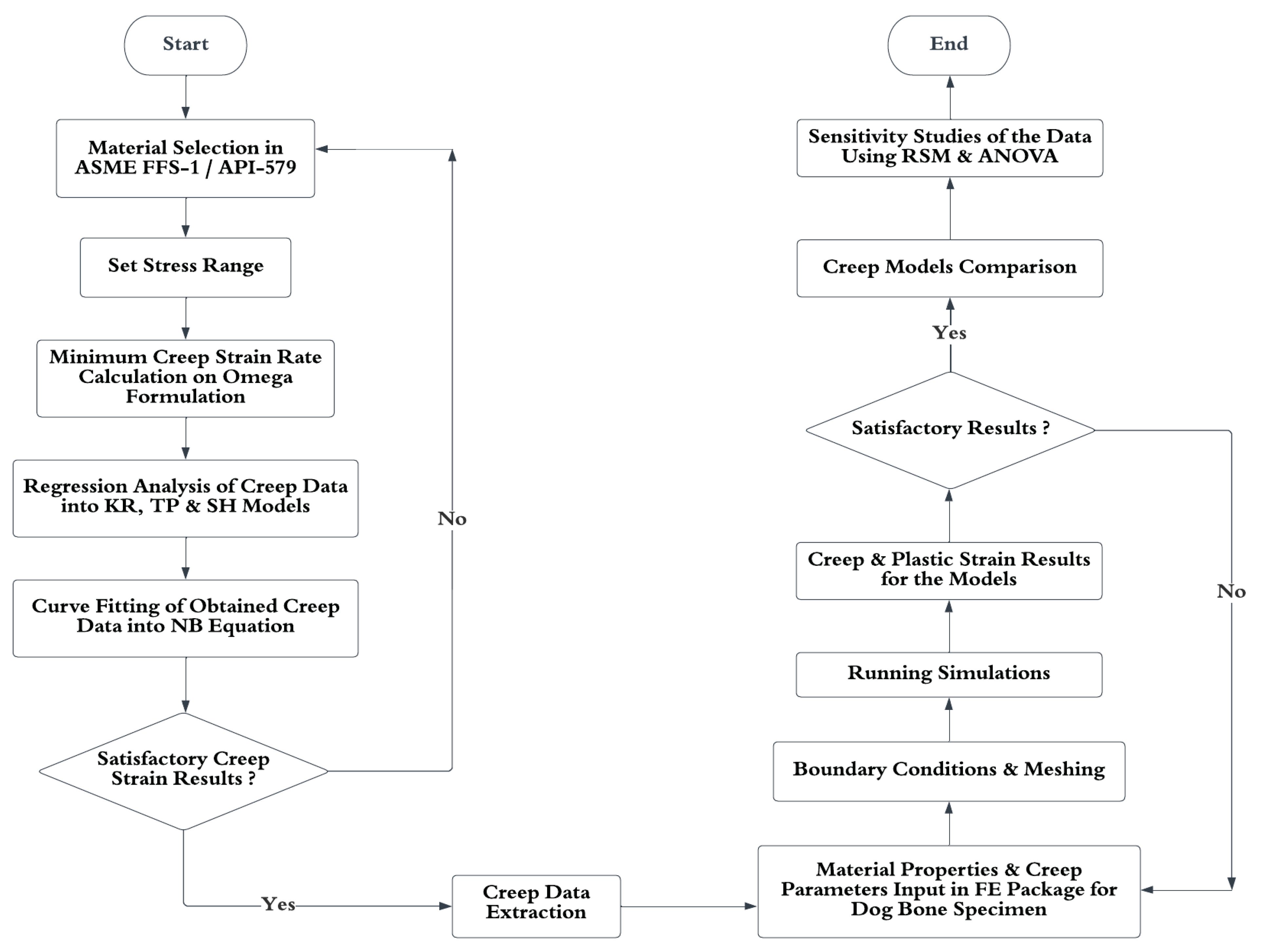
As indicated in Equation (17), the steady-state/minimum creep strain rate, ${\dot{\epsilon }}_c{}_{ }$, is obtained by considering a balance in-between the hardening and the recovery mechanisms in the secondary stage of creep analysis [13]. Using McVitty’s law, the SH model was constructed to allow non-linear bending in the minimum creep strain rate vs. stress on a log–log scale [32].

$${\dot{\epsilon }}_c{}_{ }=B sinh\left(\frac{\sigma }{{\sigma }_s}\right),$$

(17)

where the constants indicate the creep coefficient and secondary creep mechanism transition stress B and ${\sigma }_s$, respectively, h(ω) is introduced into the overall creep strain rate, and h(ω) is solved for in Equation (18).

$$h(\omega )=\frac{{\epsilon }_{cr}}{B sinh\left(\frac{\sigma }{{\sigma }_s}\right)}$$

(18)

where h(ω) = exp (λ${\omega }^p)$, and λ and p are material constants that do not have a unit. Incorporating damage into Equation (18), the new equation takes the form of Equation (19).

$$\omega (t)={\{\frac{1}{\lambda } \ln [ \frac{{\epsilon }_{cr(t)}}{B sinh\left(\frac{\sigma }{{\sigma }_s}\right)} ]\}}^{1/p}$$

(19)

where ω(t) is the analytical damage calculated from the creep strain rate ${\epsilon }_{cr}$. The moment just before the cracking, time t is taken into account, t ≈ $t_r$ and $\dot{{\omega }_{cr}}$ = 1, and the creep strain becomes as shown in Equation (20):

$${\epsilon }_{cr} = {\epsilon }_{final} \approx B sinh\left(\frac{\sigma }{{\sigma }_s}\right) exp (\lambda )$$

(20)

where

$$\mathsf{\lambda }=\ln [\frac{{\epsilon }_{final}}{{\epsilon }_{min}}];{\epsilon }_{min}=B sinh\left(\frac{\sigma }{{\sigma }_s}\right)$$

(21)

The symbol λ represents a material constant that can be calculated directly from the available experimental data for this case. The ideal value for p was suggested here to be 3/2 units less than the value of λ. Appropriately, the creep strain rate of the sin-h model is given by Equation (22). In this scenario, it is possible to derive the material constant (λ) directly from experimental data. According to this theory, p should be 3/2 units less than the actual number. Equation (22) represents the sin-h model’s creep strain rate [33].

$${\epsilon }_{cr}=B sinh\left(\frac{\sigma }{{\sigma }_s}\right) exp\left(\lambda {\omega }^{\frac{3}{2}}\right)$$

(22)

The five models’ mathematical formulations were compared by a correlation method in the article in order to systematically assess the outcome of the research study. ANOVA and response surface methodology tools were implemented for the correlation study and to measure the significant contribution of the factors on the target response, i.e., the creep strain rate in this case, by applying the models for creep response and prediction.

3. Methodology

The analytical creep strain and strain rate were first calculated by regression analysis of creep plots through an extrapolative prediction of the models. The TP, KR, and SH creep damage models were curve-fitted to NB models in the computational analysis by standardizing them with the baseline Omega model. The results were afterwards compared with the models, with the statistical data analysis executed through response surface methodology (RSM) and analysis of variance (ANOVA). The regression equations were modified accordingly for every model to extract the creep data. The overall methodology flowchart is depicted in Figure 1.

Finite element modelling and geometry were then created in the FE package Abaqus for dog-bone specimens based on an elastic–perfectly plastic model. The SS-304 dog-bone specimen’s material and physical characteristics were taken from ASME BPVC section II, subpart D [34]. The simulations were computed for each model by integrating the material constants of the creep parameters and stress exponents under the user-defined boundary conditions and meshing. Direct comparisons of the creep and plastic strain results were analyzed for each model to quantify the characteristics at different operating temperatures, pressure, and loading conditions for the SS-304 material. Sensitivity analyses were then performed to consider the uncertainties in the data analysis.

3.1. Creep Strain Analytical Analysis

Creep strain and the creep strain rate were calculated analytically for the SS-304 FE dog-bone specimen using Omega’s creep baseline material model, which is based on API-579/ASME FFS-1 standards [35]. Curve-fitting was utilized for the SS-304 material model to convert the stress exponent (n) and the creep parameter (A) obtained by regression for the KR, Omega, TP, and SH models to the embedded Norton–Bailey model available in the Abaqus material library.

Table 1. Material coefficients for the SS-304 material type from MPC Omega (MPa, °C) [35].

	$\mathbf{Parameter} \mathbf{Strain} \mathbf{Rate}—\left({\mathit{\epsilon }}_{\mathit{c}0}\right)$		Parameter Omega—(Ω)
Type-SS 304	A0	−19.17	B0	−3.40
	A1	37,917.40	B1	10,521.29
	A2	−12,389.36	B2	−7444.83
	A3	4112.12	B3	3266.58
	A4	−936.22	B4	−552.00

shows the factors that were employed in the analytical calculations to determine typical material behavior. Coefficient values were reserved from the API-579/ASME FFS-1 standards [35] after a detailed examination of the material behavior. The coefficients and material properties were selected from the defined standards to standardize the established models for comparison and analysis.

The parameters and formulations for the MPC Omega model are explained in the API-579/ASME FFS-1 standards. Using the material coupon SS-304 dog-bone specimen, the analytical creep strain was computed based on the API-579/ASME FFS-1 standards [35] and utilizing the closed-loop Equations (23)–(30) that were designed and included in the standards for the Omega model.

$${\log }_{10 }\left[\dot{{\epsilon }_{c0}}\right]=-[ (A_0 + {\Delta }_{\Omega }^{sr}) + (\frac{A_1+A_2{S}_1 +A_3{S}_1^2+A_4{S}_1^3 }{T_{ref} + T}) ],$$

(23)

$${\Omega }_m={\Omega }_n^{{\delta }_{\Omega +1}} + {\alpha }_{\Omega }+n_{BN},$$

(24)

$${\Omega }_n = max\mathit{[}\mathit{(}\Omega - n_{BN},3\mathit{)}\mathit{]},$$

(25)

$${\log }_{10 }\left[\Omega \right] = \left[\right(B_0 + {\Delta }_{\Omega }^{cd})+(\frac{B_1+B_2{S}_1 +B_3{S}_1^2+B_4{S}_1^3 }{T_{ref} + T})$$

(26)

$${\delta }_{\Omega } = {\beta }_{\Omega }.(\frac{{\sigma }_{1 }+{\sigma }_{2 }+{\sigma }_3}{{\sigma }_e}-1),$$

(27)

$$n_{BN } = -(\frac{A_2+2A_3{S}_1 +3 A_4{S}_1^2 }{T_{ref} + T}),$$

(28)

$$T_{ref} = 460 for °F\mathit{;} T_{ref} = 273 for °C$$

$${\sigma }_e = \frac{1}{\sqrt{2}} {\left[{\left({\sigma }_1-{\sigma }_{2 }\right)}^2+{\left({\sigma }_1-{\sigma }_{3 }\right)}^2+{\left({\sigma }_2-{\sigma }_{3 }\right)}^2 \right]}^{1/2},$$

(29)

$$S_1 = {\log }_{10 }\left[{\sigma }_e\right].$$

(30)

3.2. Regression Analysis of Creep Plot through Extrapolative Prediction

The MPC model Omega was utilized for inelastic analysis in the API-579/ASME FFS-1 creep evaluation standards. The dog-bone FE geometry was developed based on the ASTM standards and the Omega-NB regression model, as depicted in Figure 1, for the process flow for obtaining the creep data [24]. The data was then uploaded into the FE analysis software along with additional parameters to calculate the plastic strain and creep results [31].

The procedure details are explained with the Omega model; the creep strain values can be obtained using Equation (8). The MPC Omega model’s strain rate was stress- and temperature-dependent [23]. The strain rate can be computed by treating the temperature as constant. As previously explained, the strain rate was then calculated using the NB creep model, Equation (3). Given that it is based on the creep power-law, using the power-law regression equation for the NB model was a wise choice [36].

The curve-fitting for varying loads and temperatures could then be accomplished by comparing the generic power-law regression equation to the NB power-law [22]. For the analysis example, the extrapolation assumed that the existing trend in the material’s behavior would continue along with time. For each established model used in this research, the regression Equations (31) and (32) were modified accordingly to calculate the creep parameters and the stress exponent for each model and by introducing a damage evolution parameter to model the tertiary creep damage of the SS-304 material [35].

$$n=\frac{i\sum \left(\ln \sigma \ln \dot{\epsilon }\right)-\sum \left(\ln \sigma \right)\sum \left(\ln \dot{\epsilon }\right)}{i\sum \left[\left(\ln \sigma {)}^2\right]-\right[(\sum \left(\ln \sigma {)}^2 \right]}$$

(31)

$$A=e^{\frac{\sum \left(\ln \dot{\epsilon }\right)-n\sum \left(\ln \sigma \right)}{i}}$$

(32)

where the creep parameter is A, the stress exponent is n, and the sample size is i.

Graphical representations of the strain rate vs. stress from Omega to NB and Omega to the other models developed from the curve-fitting procedures are shown in Figure 2. The curve-fitting for the provided stress–strain values was observed to be accurate. Particularly for exponential data, the power-law regression delivered an accurate fitting [26]. An acceptability criterion for the prediction plot was a coefficient of determination R² value of 0.9803, which was significantly higher than the criterion set by the ASME FFS-1/API-579 standards for this plot. To assess the effects of material degradation at the tertiary stage of creep for the SS-304 material, the tertiary creep damage constant (ω) was derived in the regression equations [22].

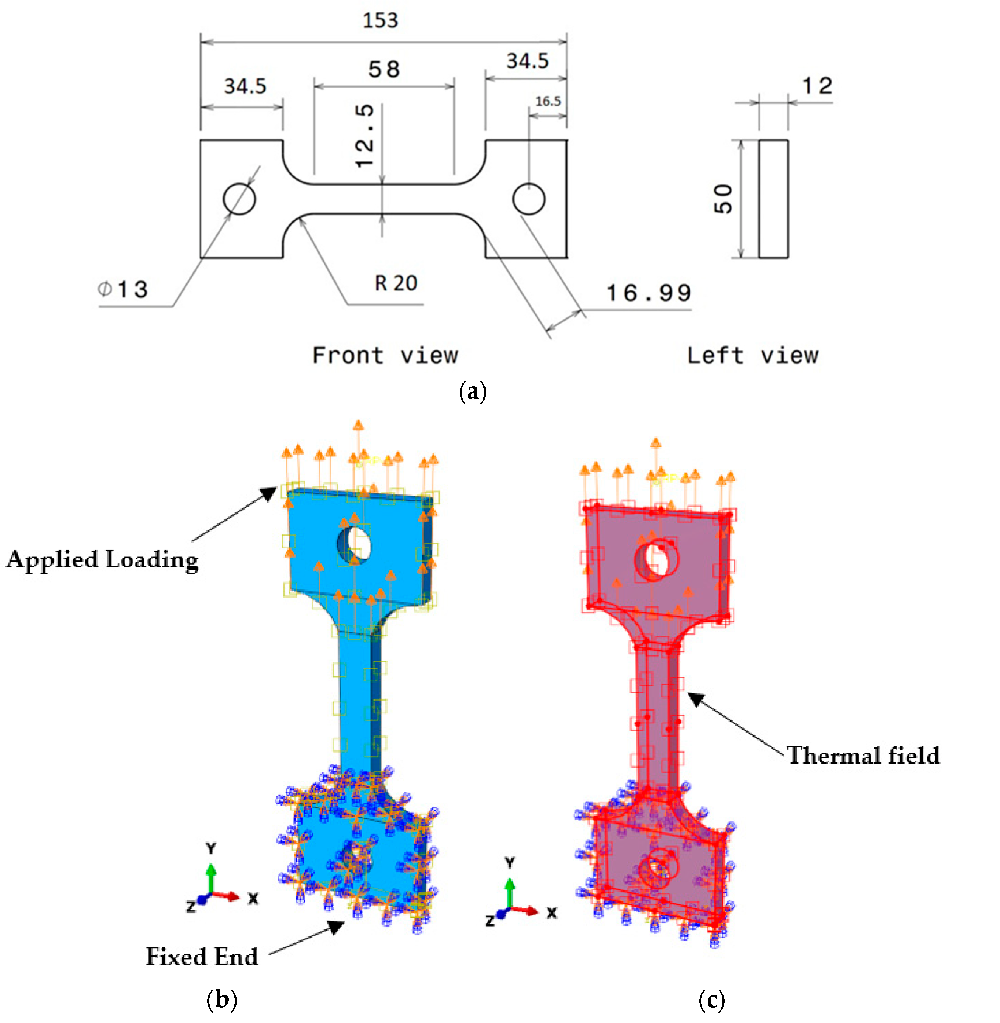
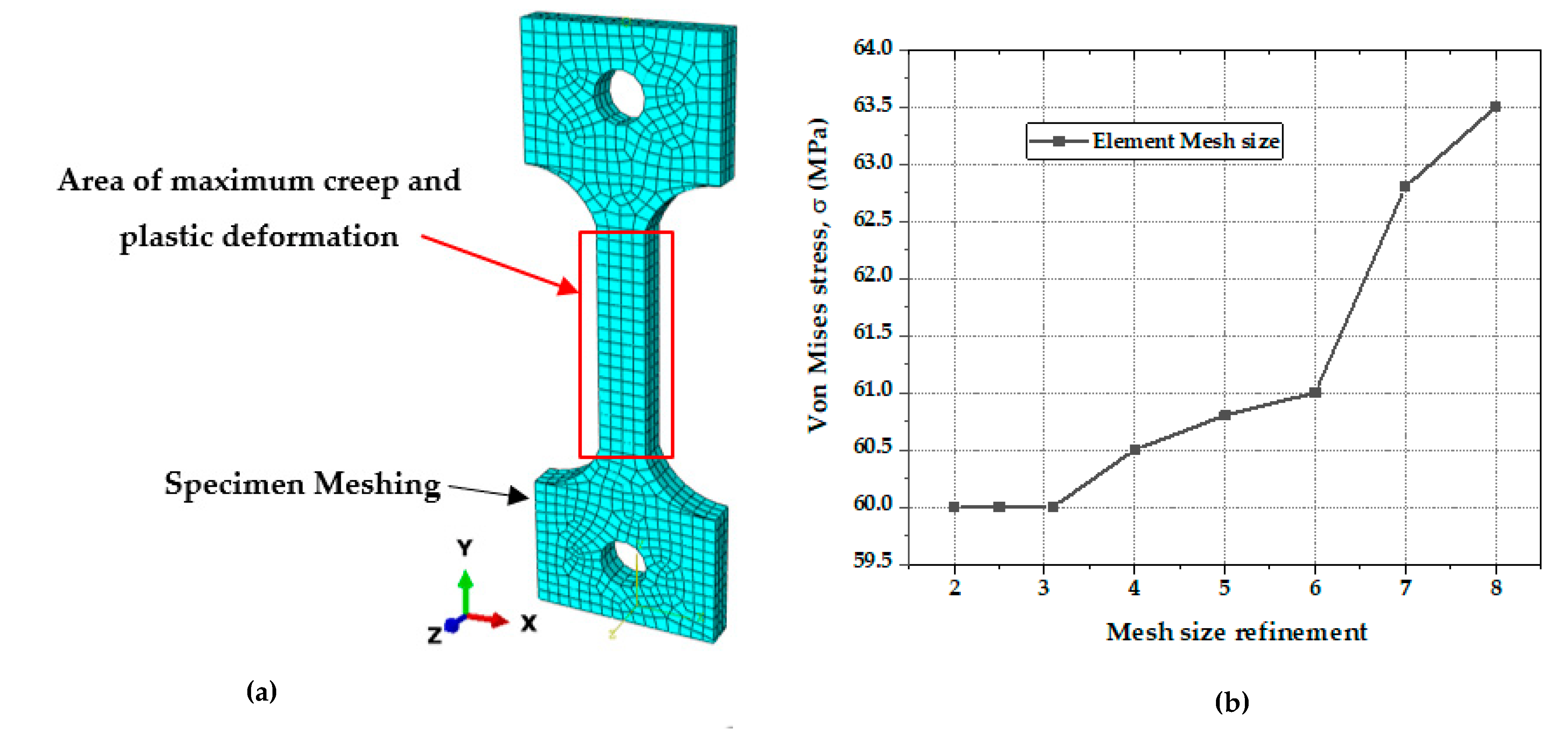
3.3. Finite Element Geometry Modelling and Pre-Processing

The FE model of a dog-bone geometry was developed as per the ASTM E-139 tensile creep testing standards [37], as shown in Figure 3a. The analyzed data had a maximum of 100 increments and an 18,000 h increment [36]. The creep deformation was modeled using the Omega–Norton–Bailey regression model. The FE dog-bone model results were first obtained for the Omega model, which was taken as the baseline model for model comparison in this research study [37]. The same FE model was then utilized for obtaining the creep damage data and to run the FE simulations while implementing other mathematical models. Consequently, the simulations were run separately for all the creep damage models, but the FE dog-bone model geometry remained the same for running the simulations and for the analysis. The same pre-defined boundary conditions were implemented for each model, and the material’s deformation behavior was observed to be different for every creep model.

Based on the assumptions employed in the analysis, the isotropic material SS-304 was chosen for the assessment. Under particular boundary circumstances and in the presence of a thermal field, a uniaxial force was applied to the specimen. An elastic–perfectly plastic model was chosen to simulate the plasticity, plastic deformation, and elasticity [38]. The displacement was measured at one end of the specimen with a 2 mm/min amplitude and was fixed at the other end. By applying particular thermal fields across the model at temperatures ranging from 0 to 700 °C for the SS-304 material, a thermal environment was created. A steady longitudinal load was applied once the desired temperature was obtained, inducing dislocation and distortion in the material’s grain structure. The load was maintained for the analysis duration or until the specimen ruptured with a 35% UTS load of standard pre-stress. Figure 3b,c depicts the specimen for the boundary conditions and thermal analysis, as the pre-defined temperature field with direct specification was instantaneous and kept constant throughout the region up to 720 °C for running the simulations that were defined in Abaqus [39].

The simulation involved is a case of creep visco-plastic behavior with the boundary conditions of one end fixed and a uniaxial load being applied to the other end. The simulations were run while applying the creep models one by one for the same thermal boundary and stress conditions applied to the same FE dog-bone specimen for the comparison of the models [40]. Meshed geometry was used to construct the thermal environment with the pre-defined boundary conditions. The area of maximum creep deformation is highlighted in red in the figure, where the maximum concentration of the applied load resulted in specimen deformation due to creep. After conducting the mesh convergence study, an element mesh size of 3.1 gave accurate results with less computational time, and the number of elements selected was set at 1713 [33]. The graph in Figure 4a depicts the selection of a suitable mesh size while performing the mesh convergence study shown in Figure 4b.

The isotropic material SS-304′s material properties, Young’s modulus, and Poisson’s ratio were obtained from ASME BPVC section II, part D, subpart 2 [34]. The physical properties of the SS-304 material, plastic strain for plasticity, and yield stress standards were also obtained from ASME BPVC section II, part D, subpart 2 [34]. The thermal conductivity, density, and thermal expansion coefficient were also obtained from the standards for creating the thermal environment for the simulation, as tabulated in

Table 2. Material and physical properties of SS-304 material [34].

Material Model	Elastic–Perfectly Plastic
Young’s modulus	(201,000–17,100) MPa @ −25 °C to 720 °C
Poisson’s ratio	0.31
Density	8000 kg/m3
Thermal expansion coefficient	17.3 × 10−6 °C−1
Thermal conductivity	16.2 W m−1 °C−1
Yield stress	(207–126) MPa
Plastic strain	(0–0.015)

.

For the material constants in the models involving NB, KR, SH, and TP, the creep parameters and stress exponents were calculated using curve-fitting for the damage progression and regression analysis [22]. The values of the creep parameter and the exponent for stress are shown in

Table 3. Material constants for SS-304 for creep models at (680–720) °C and (20–60) MPa.

	Norton–Bailey Model	Kachanov–Rabotnov Model	Sin-h Model	Theta Projection Model	Temperature (°C)
Creep parameters	1.93 × ${10}^{-18}$	2.10 × ${10}^{-18}$	4.71 × ${10}^{-15}$	2.47 × ${10}^{-15}$	680
	4.71 × ${10}^{-18}$	5.15 × ${10}^{-18}$	1.06 × ${10}^{-14}$	8.24 × ${10}^{-15}$	690
	1.13 × ${10}^{-17}$	1.23 × ${10}^{-17}$	2.35 × ${10}^{-14}$	2.68 × ${10}^{-14}$	700
	2.67 × ${10}^{-17}$	2.90 × ${10}^{-17}$	5.13 × ${10}^{-14}$	8.51 × ${10}^{-14}$	710
	6.18 × ${10}^{-17}$	6.73 × ${10}^{-17}$	1.10 × ${10}^{-13}$	2.64 × ${10}^{-13}$	720
Stress exponent	7.10	7.08	7.11	7.91	680
	7.03	7.01	7.03	7.65	690
	6.69	6.94	6.96	7.40	700
	6.88	6.87	6.89	7.16	710
	6.82	6.80	6.82	6.92	720

. Tertiary-stage creep and material behavior until rupture were considered when determining the values to model the primary, secondary, and tertiary creep curves.

3.4. Sensitivity Analysis of Established Models Using RSM and ANOVA

In these case studies, the creep strain model was built using the response surface methodology (RSM) by analyzing the simulation results with the Design-Expert software version 12. The corresponding design matrices for the established models were developed using a central composite design (CCD), taking into account four independent design factors, namely stress (A), the exponent for stress (B), the creep parameter (C), and the damage parameter (D), with one response (strain rate) being reported in

Table 4. Independent design factors and response for RSM.

			Independent Design Factors				Response
	Models	Values	Stress (A) MPa	Stress Exponent (B) ‘n’	Creep Parameter (C) MPa−nh−1	Damage Parameter (D) ‘ω’	Strain Rate 10−5/h
Norton–Bailey		Low	3	6.82	1.93 × ${10}^{-18}$	0	1.11 × ${10}^{-8}$
		High	81	7.16	6.18 × ${10}^{-17}$	0	15.89
Theta Projection		Low	3	6.72	8.24 × ${10}^{-15}$	0.05	8.71 × ${10}^{-9}$
		High	81	8.11	2.64 × ${10}^{-13}$	0.40	17.28
Kachanov–Rabotnov		Low	3	6.66	5.15 × ${10}^{-18}$	0.05	3.83 × ${10}^{-7}$
		High	81	7.08	1.23 × ${10}^{-17}$	0.40	521.65
Sine-Hyperbolic		Low	3	6.68	1.10 × ${10}^{-13}$	0.05	1.99 × ${10}^{-5}$
		High	81	7.25	4.71 × ${10}^{-15}$	0.40	11.74

[38]. Sensitivity studies were carried out on the results to quantify the effect of the uncertainties for the response output against the variable inputs.

As the analytical Omega model was considered and used for the curve-fitting of the other models, an RSM analysis was not applied to the model. In the case of the Norton–Bailey model, as the damage parameter factor was not available, the creep and damage parameters were not considered in the analysis. The independent variables exhibited a non-linear connection with the response variable, strain, which was a source of non-linearity in the considered models [41]. The quadratic models best described the correlations among the independent components and the response variable in these circumstances [42].

The quadratic models were determined to be significant based on the statistical analysis, with a coefficient of determination R² value of more than 80%. Once the appropriate model was selected, the evaluation involved 3D surface plots showing the connection between the design components and the outcomes. These graphs were used to understand how all of the responses behaved and correlated to each other. The optimization criteria for each design parameter were then specified with a suitable significance. The ideal values of the design parameters were established in the following surface plots. Analysis of variance (ANOVA) was also used to assess the differences between two or more means and variables through significance tests. For each model, design matrices with 30 simulation runs were created after assigning low and high values to specified factors. To increase the dependability of the design and analysis, these matrices also included replicas of the core points [43].

4. Results and Discussions

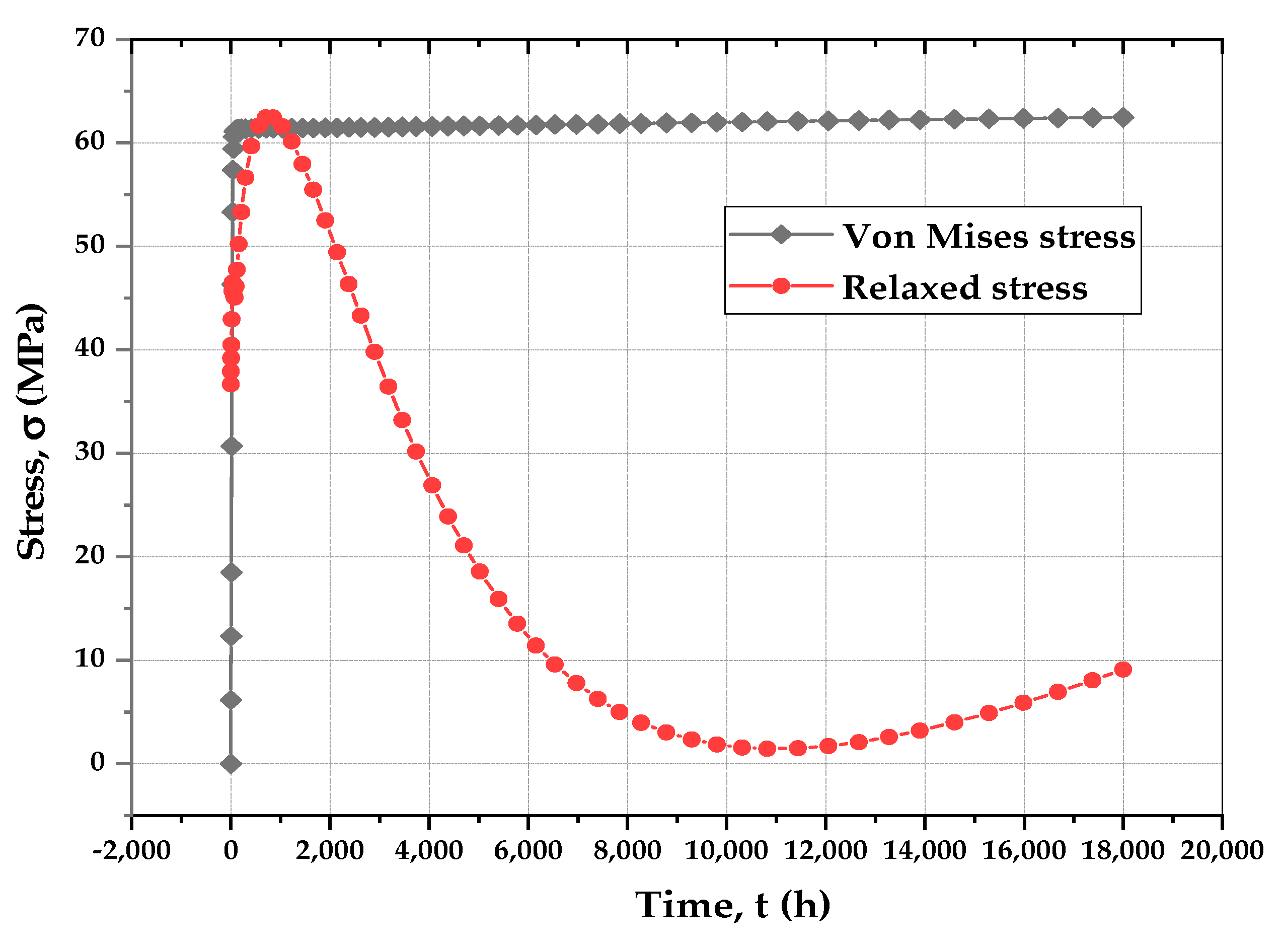
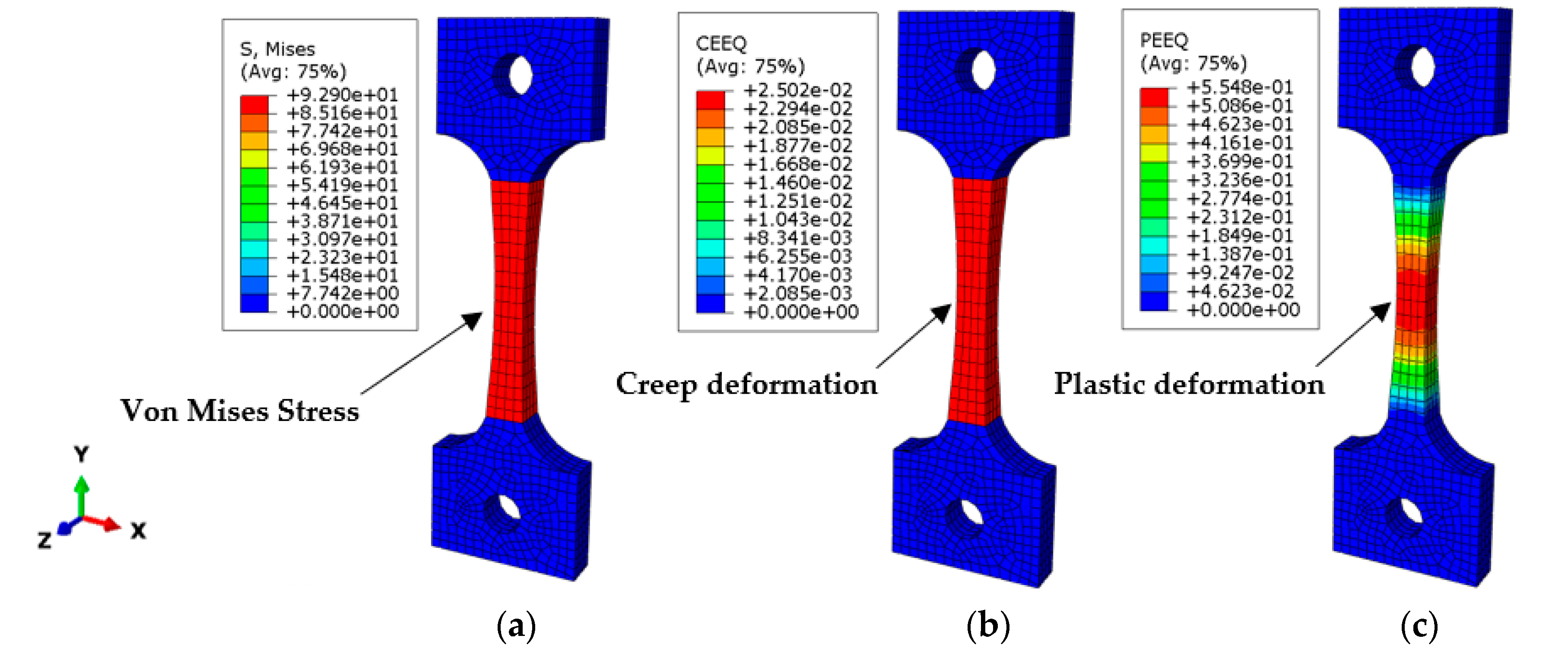
4.1. FE Analysis of Dog-Bone Specimen of SS-304

The creep models were applied to the dog-bone model of SS-304 using regression analysis, as discussed in the previous section. Following a simulation of 18,000 h under the given boundary conditions for creep using the built-in Norton–Bailey model, Von Mises stresses were extracted from the model. As the time progressed, the induced stresses gradually decreased from 60 MPa to around 10 MPa and approached zero, which lasted until the end of the 18,000 h visco-elastic–plastic cycle, as shown in Figure 5. The relaxed stresses decreased as a result of the specimen’s induced strain [40]. Relaxed stresses were created as the model was subjected to creep strain as a result of ongoing plastic deformation and rupturing. Other creep models were also applied to the same model geometry to attain the respective results.

The material’s yield stress and ultimate tensile strength were surpassed by the continuous loading, which caused cracking. To show creep, the FE model of the SS-304 specimen was subjected to uniaxial tensile stress to demonstrate the creep damage. Deformation occurred in the middle of the specimen, which was fixed using symmetric boundary conditions. Figure 6a displays the specimen’s Von Mises stress distribution after running the simulations to obtain the creep deformation [44]. Significant stresses were created at the free end and at the center, whereas lesser stresses were distributed around the specimen’s fixed end. The material began to deform as soon as the load was applied. It transitioned from an elastic to a plastic state under the effect of the temperature environment and specified boundary conditions. For the imposed stresses, Figure 6b,c shows the creep and plastic strain in the specimen. The following sub-sections discuss the comparison of the models for creep deformation.

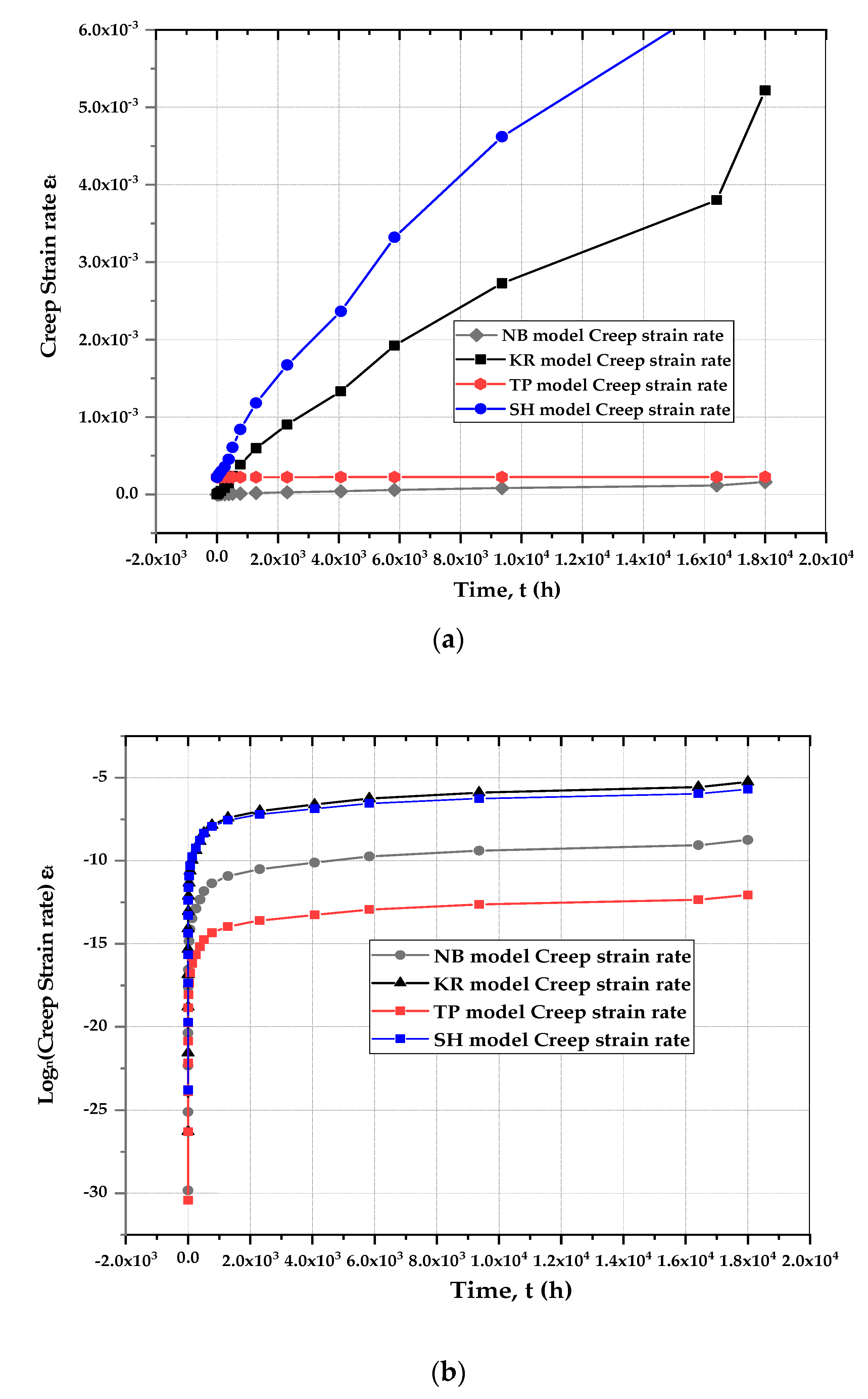
4.2. Model Comparison—Minimum Creep Strain Rate

The minimum creep strain rate was calculated using Norton‘s power law in the KR model as opposed to the McVitty’s sine-hyperbolic law in the SH model. Creep power laws were also used in the development of the Omega and TP models. The ability of the KR and SH models to predict the minimum creep strain was also examined. These rules were calibrated using five isotherms of the minimum creep strain rate data from the simulations. Figure 7a depicts these five models’ creep strain rate predictions at 720 °C and 60 MPa. Figure 7b was plotted while taking the natural logs of the creep strain rates to smoothen the models’ curves. When the simulation data was examined, it was discovered that the 680 °C, 690 °C and 700 °C isotherms were non-linear, whilst the 710 °C and 720 °C isotherms were linear. The sigmoidal behavior shown in the simulations and tests could not be accurately replicated by the KR rupture predictions since they were linear on a log–log scale [45]. The KR model can be re-calibrated to handle either high- or low-stress scenarios, but not both at the same time [46]. The NB, Omega, and TP models all had the same problem of being unable to forecast sigmoidal behavior at higher isotherms. The SH rupture predictions could successfully model the sigmoidal behavior and bend on a log–log scale. The constant σ_s regulates the bend in the SH model. Compared to the KR, NB, Omega, and TP models, the SH model better fit the simulation data over a wide range of stresses. When the applied stress range was constrained, the KR model performed well compared to the other models.

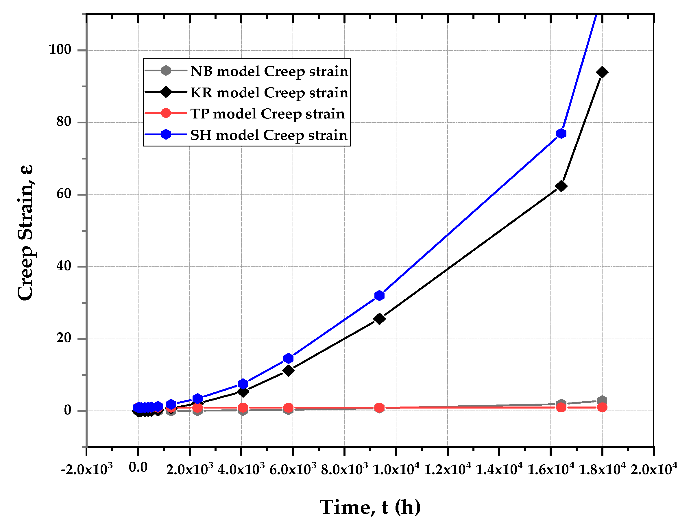
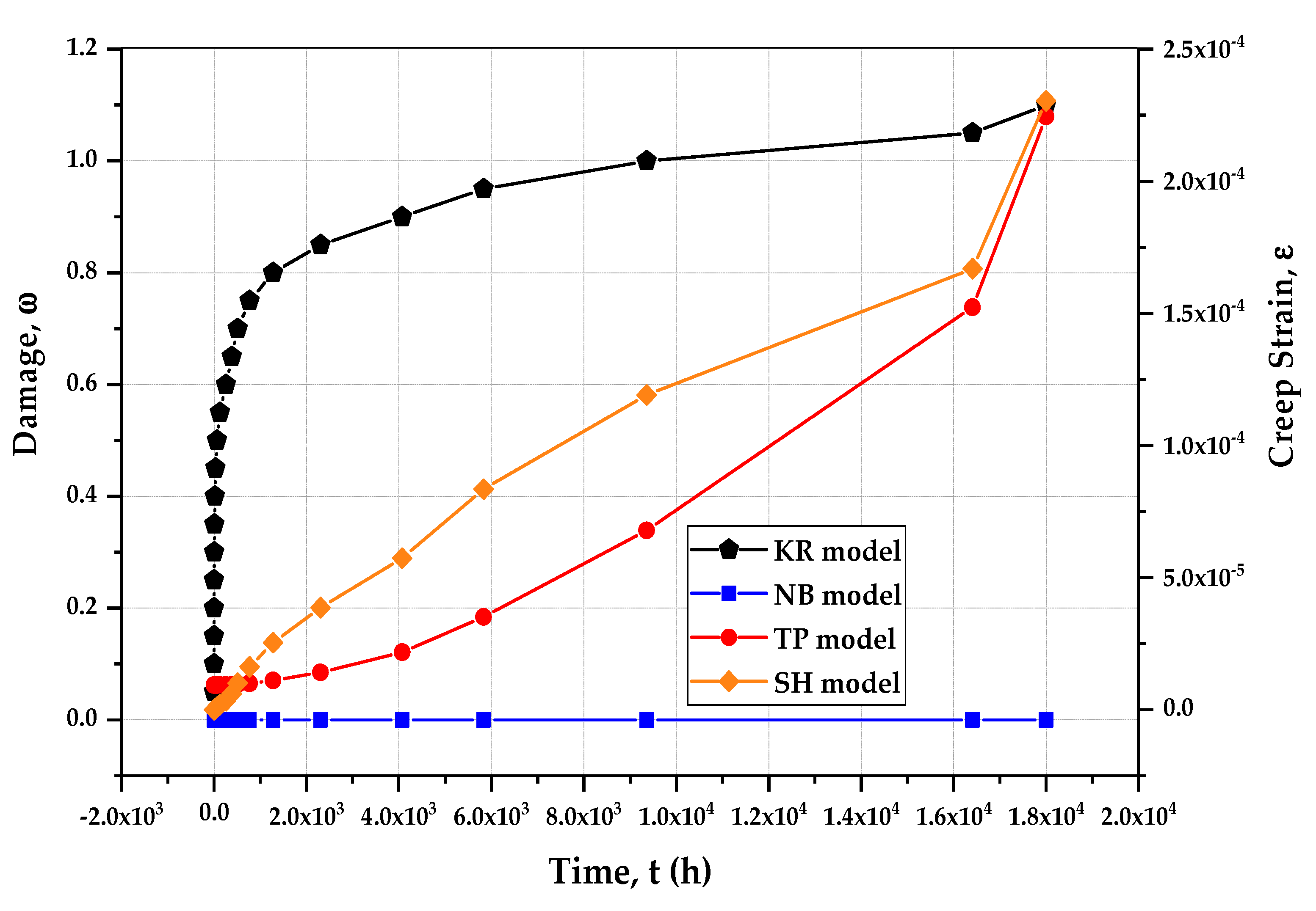
4.3. Model Comparison—Creep Deformation and Damage

The KR, sin-h, and Theta models could simulate the complete creep deformation curve, including the secondary and tertiary creep regimes. However, the Omega and Norton–Bailey models were deficient in predicting the entire creep curve [47], as depicted in Figure 8. Using the simulated data, it was observed that all the models could accurately forecast the creep deformation of the SS-304 material. While the ductility and rupture time differed slightly between the models, this was not sufficient for declaring one model superior to the other [48]. There were three aspects to the damage evolution prediction: critical damage, rupture time, and the damage rate [49]. For the provided creep curves, the KR, Theta, and sin-h models anticipated identical rupture periods; however, the critical damage and damage trajectory differed. The NB and Omega models were not intended to estimate the damage evolution during the material’s tertiary creep stage. Using the analytical damage calculation, it was discovered that the critical damage in the KR and Theta projection models had a range from 0.2 to 0.3, meaning that the rupture occurred when the damage was substantially less than unity. The theory of continuum damage mechanics (CDM) contradicts this, as it highlights that the damage trajectory is nearly infinitely long as it approaches rupture [50]. The critical damage in the sin-h model always resolved to unity due to the material constant λ. As a result, the damage trajectory was always finite toward rupture [51].

4.4. Model Comparison—Stress-Rupture

The stress-rupture prediction was calibrated into three stress-rupture isotherms to examine the ability of the KR, Theta projection, and sin-h models to forecast stress-rupture [52], whereas the NB and Omega models lacked the ability to predict the stress-rupture curves involving damage evolution parameters. The stress-rupture predictions are shown at 720 °C in Figure 9. When the KR, Theta projection, and sin-h models were compared, it was found that the sin-h models fitted the simulation data best. The KR rupture forecast was linear on a log–log scale, allowing it to represent the region appropriately. Extrapolated rupture predictions can be used to test the physical realism of the KR, Theta, and sin-h rupture predictions.

The nominal yield strength and ultimate tensile strength of SS-304 at 720 °C were shown as a physical reality check. The sigmoidal bend was controlled by the parameter σ_t in the sin-h model. As the rupture duration approached zero, the sin-h rupture predicted bends at the yield strength and achieved a result that was less than but close to the nominal ultimate tensile strength of SS-304. Furthermore, as the rupture period approached zero, the KR rupture prediction did not bend at the yield strength. Instead, it achieved a value that was 1.35× more significant than the ultimate tensile strength. Penny [53] found that the weakness in the KR rupture prediction was caused by the “brittle curve” phenomena and revised the KR model to handle the high-stress to low-stress bend by adding additional components and material constants but kept the flaw that the critical damage is less than unity. As a result, to introduce the bend, two sets of constitutive equations were used. Near rupture, the critical damage was modest (between 0.2 and 0.4), and the damage trajectory was nearly endless. Without these additional issues and limits, the sin-h model replicated the transition from high- to low-stress regions. Figure 10 depicts the stress versus the minimum creep strain rate of the models.

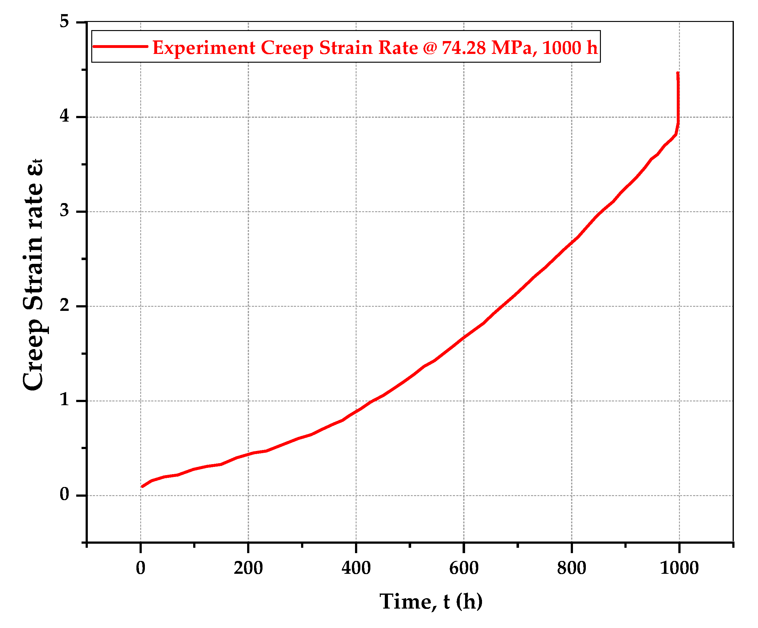
4.5. Creep Experimental Testing

The validation of the model was based on laboratory-based creep experimental testing. The tests were conducted using a 20-ton servo-control creep testing machine based on the standards as per the ASTM E-139 standards, on stainless-steel SS-304 specimens of a regular size that were firmly intact by clevis couplings and as per the standard specimen size as mentioned in Figure 3a. The temperature was controlled by a thermocouple attached to the gauge length of the specimen. Three samples were utilized for the ambient tensile tests in order to verify the yield strengths of the stainless-steel specimens. Another three samples were used to determine and confirm the ultimate tensile strength of the material. A final specimen was used to conduct the creep test. The test was conducted at 60% yield strength of the material, and the loading conditions were a pressure of 5220 MPa and a temperature of 720 °C for the creep test. The creep testing machine on which the experiments were conducted is depicted in Figure 11. The graph in Figure 12 depicts the creep strain rate for the test running up to 1000 h.

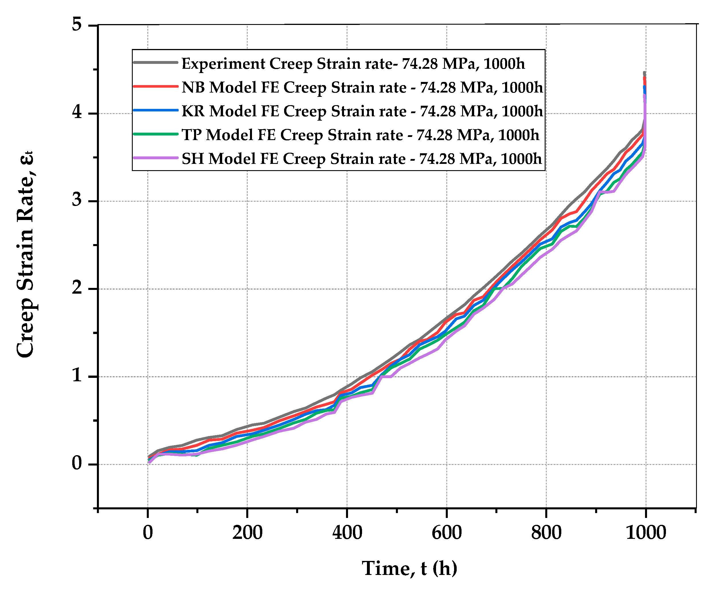
4.6. Validation of Models by Creep Experiment

The four models under study were fitted against the creep experiment data, except for the Omega baseline model, obtained for the SS-304 material at 720 °C, 74.28 MPa, and up to 1000 h. The FE numerical models’ results were compared with the real creep experiment results, as shown in Figure 13, and the maximum percentage error deviation between the FE and creep experiment results were calculated and are tabulated in

Table 5. Maximum percentage deviation between FE and creep experiment results for the models.

Type of Creep Test	Creep Models	Maximum Deviation up to 5%
		FEA	Experiment
1000 h	NB Model	0.1596	0.0994
	KR Model	0.2282	0.0994
	TP Model	0.2878	0.0994
	SH Model	0.3332	0.0994

. A maximum deviation of up to 5% for the selected points, taken as a reference between the FE and creep experiment results, was found to be minimum. The FE simulations were later extrapolated to 18,000 h for the models to complete the analysis.

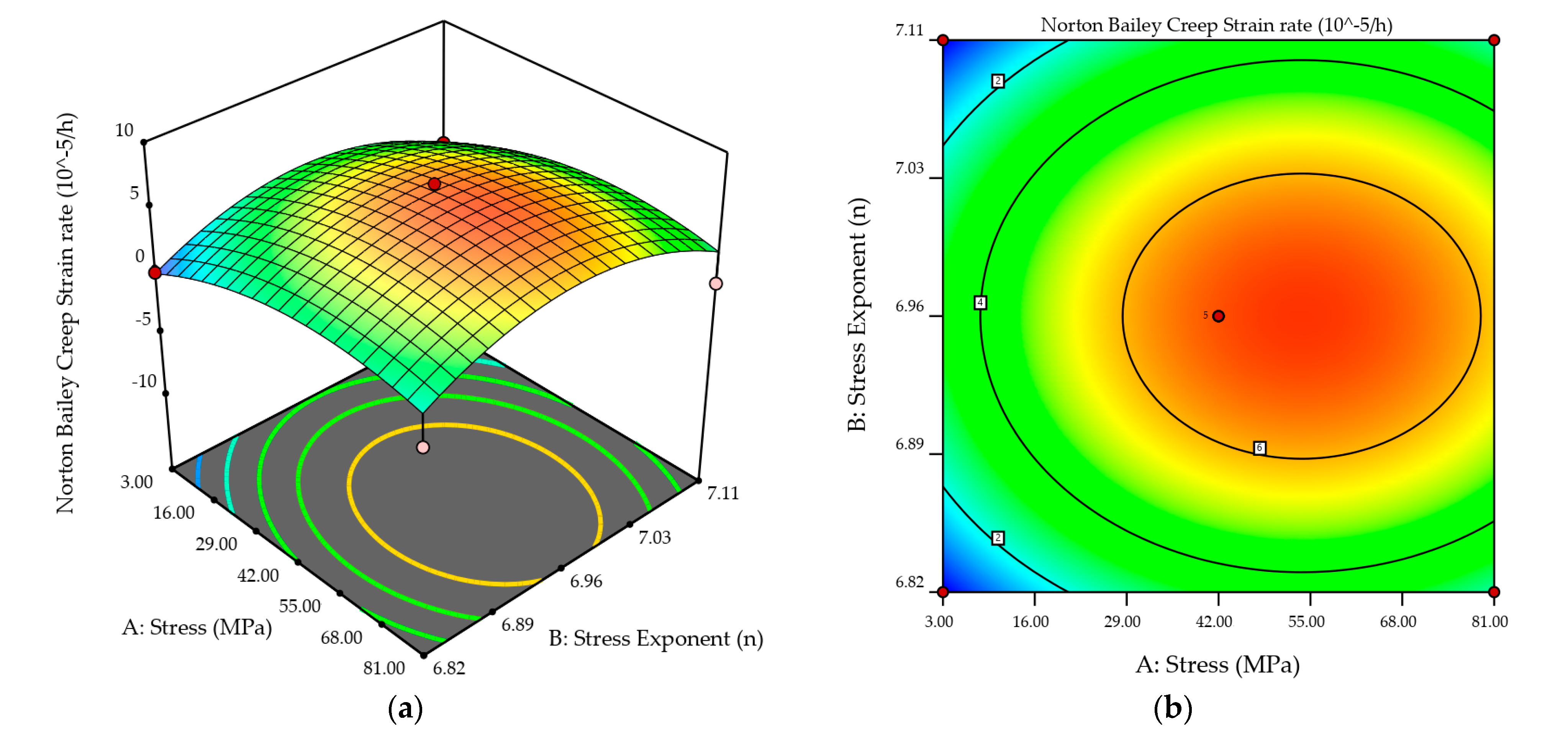
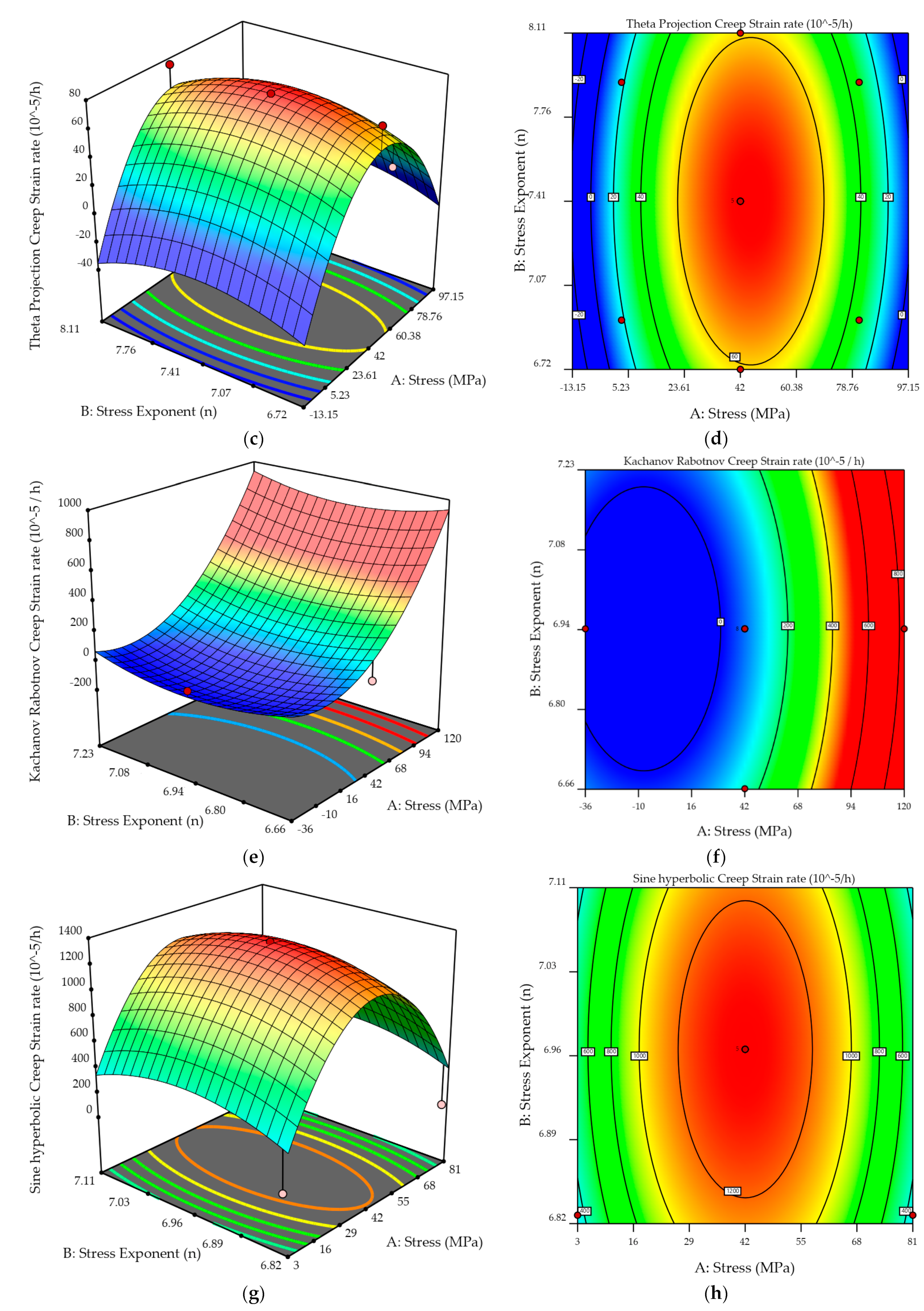
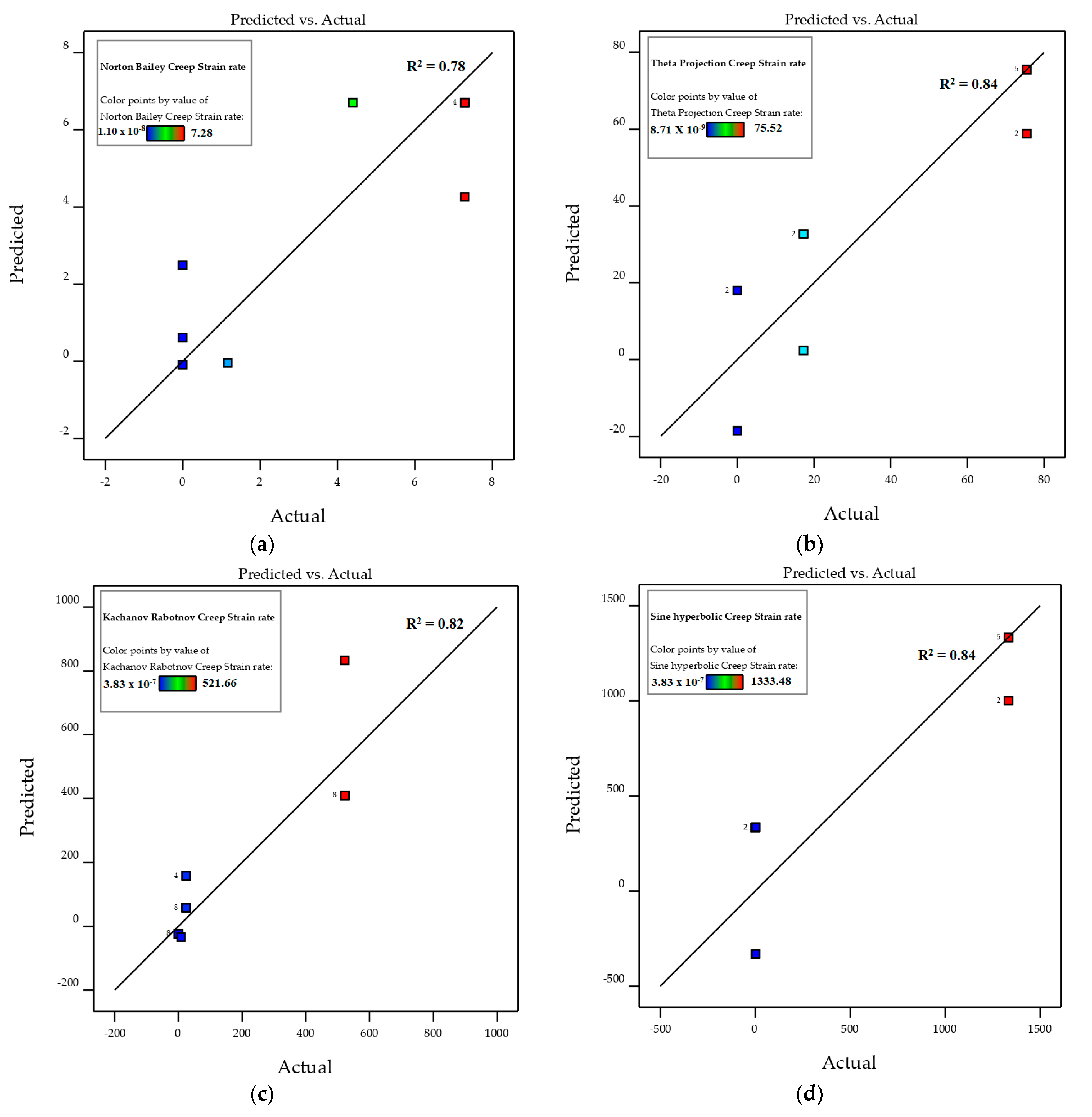
4.7. Data Optimization by Statistical Modelling

For the response analysis, the quadratic regression models were chosen for statistical analysis of the response strain. The regular coefficient of determination (R²), modified coefficient of determination (adjusted R²), and expected coefficient of determination (predicted R²) for each example were used to verify the applicability of the selected regression models. Table 5 displays the fit statistics for the response strain produced from a central composite design. The relevance of the models can be seen in the R² values. Furthermore, the modified R² and anticipated R² values were close to each other. The term “adequate precision” refers to the comparison between the predicted values, referred to as “signal,” and the average prediction error is referred to as “noise”. The models’ performance is shown by the suitable relationship between the signal and noise. It was found that all the quadratic models were significant for searching the design space [54].

The projected vs. actual responses were displayed to verify the appropriateness of the generated models. The graph shows that the predicted and actual values for the concerned reaction were very close. The distribution of the data points along the run order implies that the values predicted by the model did not change much [55]. With random dispersal, most of the values were close to the middle line. In this situation, there was no discernible pattern of residuals above and below the central line, establishing that the run order of the design procedure did not affect the data; consequently, the model was significant [56]. The statistical characteristics and synergistic effects of each constituent were determined by using ANOVA. The regression model’s applicability and suitability were recommended by various ANOVA adequacy tests (the F-value, the lack of fit, and the p-value) [57]. Figure 14a–d shows the plot of the interaction and correlation analysis for each model between the parameters stress and stress exponent on the response strain, which was also manifested in the mathematical model equations.

Table 6. Fit statistics of the models.

Fit Statistics for NB Model’s Creep Strain Rate (εt)
Statistical Parameters	Values
R2	0.78
Adjusted R2	0.62
Predicted R2	−0.29
Adequate precision	4.71
Fit Statistics for TP Model’s Creep Strain Rate (εt)
R2	0.84
Adjusted R2	0.74
Predicted R2	−0.07
Adequate precision	7.72
Fit Statistics for KR Model’s Creep Strain Rate (εt)
R2	0.82
Adjusted R2	0.74
Predicted R2	0.26
Adequate precision	12.60
Fit Statistics for SH Model’s Creep Strain Rate (εt)
R2	0.84
Adjusted R2	0.73
Predicted R2	−0.10
Adequate precision	6.88

illustrates the fit statistics of the models and

Table 7. Summary of the models.

Response: NB Model’s Creep Strain Rate—Model Summary
Source	Std. Dev.	R2	Adjusted R2	Predicted R2	Press
Linear	3.62	0.09	−0.08	−0.54	222.62
2FI	3.81	0.09	−0.21	−1.73	393.94
Quadratic	2.12	0.78	0.62	−0.29	186.96	Suggested
Cubic	1.91	0.87	0.69	−4.20	750.21	Aliased
Response: TP Model’s Creep Strain Rate—Model Summary
Linear	38.04	0.02	−0.16	−0.81	27,007.75
2FI	40.09	0.02	−0.29	−1.99	44,564.25
Quadratic	17.93	0.84	0.74	−0.07	15,998.53	Suggested
Cubic	21.15	0.84	0.63	−8.60	1.43 × 105	Aliased
Response: KR Model’s Creep Strain Rate—Model Summary
Linear	138.51	0.69	0.65	0.58	6.73 × 105
2FI	147.27	0.69	0.61	0.48	8.34 × 105
Quadratic	119.07	0.82	0.74	0.26	1.18 × 106	Suggested
Cubic	108.94	0.88	0.78	−6.52	1.22 × 107	Aliased
Response: SH Model’s Creep Strain Rate—Model Summary
Linear	757.0	0	−0.20	−0.86	1.07 × 107
2FI	797.95	0	−0.33	−2.08	1.76 × 107
Quadratic	356.15	0.84	0.73	−0.10	6.31 × 106	Suggested
Cubic	421.41	0.84	0.62	−8.91	5.68 × 107	Aliased

demonstrates the summary of the models, the relative error, and the significance of the models.

The following three-dimensional plots provided an assessment of behavior of the response and revealed the independent elements’ synergistic effects on the chosen response. In general, the 3D model showed the answer as a function of two independent components, with the remaining two elements being held constant at their mean coded values. The functional connection between the defined dependent variables and the associated independent variables was illustrated using three-dimensional surface plots. The response surface plot in Figure 15a,c,e,g and the contour creep deformation maps in Figure 15b,d,f,h indicate the combined impacts of the modifications. For each model, the stress exponent, creep parameter, stress, and damage parameter were measured to check their significant contributions of their impact on the target response strain [58].

The graphs of the simulation outputs with the predicted outputs for all the models are depicted in Figure 16a–d. The correlation between the predicted and actual values for the response strain rate was presented to a satisfactory level for all the models. The models did not reveal any abrupt variations in the continual variance, as indicated by their relative error values.

5. Conclusions

In this article, the TP, KR, NB, and SH models were correlated and compared through the FE modelling of the tensile specimen geometry for SS-304 material by curve-fitting the creep responses with the Omega baseline model. A direct comparison of the models’ responses was discussed through quantitative and qualitative analyses of the creep strain rate, creep deformation, damage, and rupture predictions. The analysis helped in identifying an appropriate model for the SS-304 material under the specified defined boundary conditions. The following conclusions were deduced from the study:

• The creep strain rate curve modeled by the SH model was better as compared to the KR, NB, Omega, and TP models primarily because of the material constants in its formulation. The model accurately modeled all three creep stages for the SS-304 material while running the simulation and extrapolating to 18,000 h.
• The KR, NB, Omega and TP models could not represent the minimum creep strain rate vs. stress bend accurately. However, the SH model represented the lowest creep strain rate bend precisely.
• The stress rupture predictions of the SH model exhibited a smooth curve for the creep strain and damage evolution as compared to the KR, NB, Omega, and TP models in conditions up to 720 °C and 60 MPa.
• The damage evolution differed between the KR, TP and SH models, whereas the NB and Omega models were incapable of predicting the damage evolution. The NB and Omega models depicted zero damage evolution, whereas the KR and TP models exhibited a conservative damage evolution. The best damage evolution criteria were modelled by the SH model for ω = 0–1.10.
• The combined effects of the design factors on the response SH model’s creep strain rate (ε_t) and contour creep deformation maps from the RSM results were better as compared to the other models. The relative error of the SH model’s ANOVA results was 0.84, which was comparable to the other models, which proves the significance of the model.

6. Summary

This paper compared five established creep models for their capabilities in predicting the creep deformation for stainless steel. The proposed correlation method helped in selecting the most suitable model for stainless steel creep deformation predictions for the pre-defined conditions. In comparison to the other models, the sine-hyperbolic (SH) model had various characteristics that proved its significance in predicting creep damage, creep deformation, and creep rupture for the stainless-steel SS-304 material as identified by the correlation method. The concluding results also indicated the suitability of selecting the sine-hyperbolic model over the other models from this research study and analysis.

References

1. Haque, M.S.; Stewart, C.M. Comparative Analysis of the Sin-Hyperbolic and Kachanov–Rabotnov Creep-Damage Models. Int. J. Press. Vessel. Pip. 2019, 171, 1–9. [Google Scholar] [CrossRef]
2. Sattar, M.; Othman, A.R.; Kamaruddin, S.; Akhtar, M.; Khan, R. Limitations on the computational analysis of creep failure models: A review. Eng. Fail. Anal. 2022, 134, 105968. [Google Scholar] [CrossRef]
3. Norton, F. The Creep of Steels at High Temperatures; Mc Graw Hill: New York, NY, USA, 1929; Volume 1, p. 90. [Google Scholar]
4. Bråthe, L.; Josefson, L. Estimation of norton-bailey parameters from creep rupture data. Met. Sci. 1979, 13, 660–664. [Google Scholar] [CrossRef]
5. Prager, M. Development of the MPC Omega Method for Life Assessment in the Creep Range. J. Press. Vessel. Technol. Trans. ASME 1995, 117, 95–103. [Google Scholar] [CrossRef]
6. Yeom, J.T.; Kim, J.Y.; Na, Y.S.; Park, N.K. Creep Strain and Creep-Life Prediction for Alloy 718 Using the Omega Method. J. Met. Mater. Int. 2003, 9, 555–560. [Google Scholar] [CrossRef]
7. Prager, M. The Omega Method—An Engineering Approach to Life Assessment. J. Press. Vessel. Technol. 2000, 122, 273–280. [Google Scholar] [CrossRef]
8. Kachanov, L.M. Rupture Time under Creep Conditions. Int. J. Fract. 1999, 97, 11–18. [Google Scholar] [CrossRef]
9. Christopher, J.; Praveen, C.; Ganesan, V.; Reddy, G.P.; Albert, S.K. Influence of Varying Nitrogen on Creep Deformation and Damage Behaviour of Type 316L in the Framework of Continuum Damage Mechanics Approach. Int. J. Damage Mech. 2021, 30, 3–24. [Google Scholar] [CrossRef]
10. Stewart, C.M.; Gordon, A.P. Strain and Damage-based Analytical Methods to Determine the Kachanov-Rabotnov Tertiary Creep-Damage Constants. Int. J. Damage Mech. 2012, 21, 1186–1201. [Google Scholar] [CrossRef]
11. Evans, R.W.; Parker, J.D.; Wilshire, B. The θ Projection Concept-A Model-Based Approach to Design and Life Extension of Engineering Plant. Int. J. Press. Vessel. Pip. 1992, 50, 147–160. [Google Scholar] [CrossRef]
12. Stewart, C.M. A Novel Sin-Hyperbolic Creep Damage Model To Overcome the Mesh dependency. In Proceedings of the ASME International Mechanical Engineering Congress and Exposition, Houston, TX, USA, 13–19 November 2015; pp. 1–9. [Google Scholar]
13. Alipour, R.; Nejad, A.F.; Dezfouli, H.N. Steady State Creep Characteristics of a Ferritic Steel at Elevated Temperature: An Experimental and Numerical Study. ADMT J. 2018, 11, 115–129. [Google Scholar]
14. Yang, F.Q.; Xue, H.; Zhao, L.Y.; Tian, J. Calculations and modeling of material constants in hyperbolic-sine creep model for 316 stainless steels. Appl. Mech. Mater. 2013, 457–458, 185–190. [Google Scholar] [CrossRef]
15. Yao, H.T.; Xuan, F.Z.; Wang, Z.; Tu, S.T. A review of creep analysis and design under multi-axial stress states. Nucl. Eng. Des. 2007, 237, 1969–1986. [Google Scholar] [CrossRef]
16. Haque, M.S.; Stewart, C.M. Exploiting functional relationships between MPC Omega, Theta, and Sin-hyperbolic continuum damage mechanics model. In Proceedings of the ASME 2016 Pressure Vessels and Piping Conference, Vancouver, BC, Canada, 17–21 July 2016; Volume 6A. [Google Scholar] [CrossRef]
17. Maruyama, K.; Nonaka, I.; Sawada, K.; Sato, H.; Koike, J.I.; Umaki, H. Improvement of Omega Method for Creep Life Prediction. ISIJ Int. 1997, 37, 419–423. [Google Scholar] [CrossRef] [Green Version]
18. Golan, O.; Arbel, A.; Eliezer, D.; Moreno, D. The applicability of Norton’s creep power law and its modified version to a single-crystal superalloy type CMSX-2. Mater. Sci. Eng. A 1996, 216, 125–130. [Google Scholar] [CrossRef]
19. Dyson, B. Use of CDM in Materials Modeling and Component Creep Life Prediction. J. Press. Vessel Technol. ASME 2000, 122, 281–296. [Google Scholar] [CrossRef]
20. Law, M.; Payten, W.; Snowden, K. Finite element analysis of creep using Theta projection data. Int. J. Press. Vessel. Pip. 1998, 75, 437–442. [Google Scholar] [CrossRef]
21. Cedro, V.; Pellicote, J.; Bakshi, O.; Render, M. Application of a modified hyperbolic sine creep rate equation to correlate uniaxial creep rupture data of Sanicro 25 and HR6W. Mater. High Temp. 2020, 37, 434–444. [Google Scholar] [CrossRef]
22. Sattar, M.; Othman, A.R.; Akhtar, M.; Kamaruddin, S.; Khan, R.; Masood, F. Curve Fitting for Damage Evolution through Regression Analysis for the Kachanov—Rabotnov Model to the Norton—Bailey Creep Law of SS-316 Material. Materials 2021, 14, 5518. [Google Scholar] [CrossRef]
23. Sattar, M.; Othman, A.R.; Kamaruddin, S.; Alam, M.A.; Azeem, M. Creep Parameters Determination by Omega Model to Norton Bailey Law by Regression Analysis for Austenitic Steel SS-304. Solid State Phenom. 2021, 324, 188–197. [Google Scholar] [CrossRef]
24. Sattar, M.; Othman, A.R.; Othman, M.F.; Musa, M.F. Regression Analysis of Omega Model to Norton- Bailey Law for Creep Prediction in Fitness for Service Assessment of Steel Material. Solid State Technol. 2020, 63, 1228–1239. [Google Scholar]
25. Abdallah, Z.; Gray, V.; Whittaker, M.; Perkins, K. A Critical Analysis of the Conventionally Employed Creep Lifing Methods. Materials 2014, 7, 3371–3398. [Google Scholar] [CrossRef] [PubMed] [Green Version]
26. May, D.L.; Gordon, A.P.; Segletes, D.S. The Application of the Norton-Bailey Law for Creep Prediction through Power Law Regression. In Proceedings of the ASME Turbo Expo, San Antonio, TX, USA, 3–7 June 2013; Volume 7A, pp. 1–8. [Google Scholar] [CrossRef] [Green Version]
27. Chen, H.; Zhu, G.R.; Gong, J.M. Creep Life Prediction for P91/12Cr1MoV Dissimilar Joint Based on the Omega Method. Procedia Eng. 2015, 130, 1143–1147. [Google Scholar] [CrossRef] [Green Version]
28. Stewart, C.M.; Gordon, A.P. Analytical Method To Determine the Tertiary Creep Damage Constants of the Kachanov-Rabotnov Constitutive Model. In Proceedings of the ASME, International Mechanical Engineering Congress & Exposition IMECE2010, Vancouver, BC, Canada, 12–18 November 2010; pp. 1–8. [Google Scholar]
29. Murakami, S. Continuum Damage Mechanics; Solid Mechanics and its Applications; Springer: New York, NY, USA, 2012; Volume 185. [Google Scholar]
30. Liu, H.; Peng, F.; Zhang, Y.; Li, Y.; An, K.; Yang, Y.; Zhang, Y.; Guan, X.; Zhu, W. A New Modified Theta Projection Model for Creep Property at High Temperature. J. Mater. Eng. Perform. 2020, 29, 4779–4785. [Google Scholar] [CrossRef]
31. Brown, S.G.R.; Evans, R.W.; Wilshire, B. A Comparison of Extrapolation Techniques for Long-term Creep Strain and Creep Life Prediction based on Equations Designed to represent Creep Curve Shape. Int. J. Press. Vessel. Pip. 1986, 24, 251–268. [Google Scholar] [CrossRef]
32. Haque, M.S.; Stewart, C.M. Modeling the creep deformation, damage, and rupture of Hastelloy X using MPC Omega, theta, and sin-hyperbolic models. In Proceedings of the ASME 2016 Pressure Vessels and Piping Conference, Vancouver, BC, Canada, 17–21 July 2016; Volume 6A, pp. 1–10. [Google Scholar] [CrossRef]
33. Haque, M.S.; Stewart, C.M. The Stress-Sensitivity, Mesh-Dependence, and Convergence of Continuum Damage Mechanics Models for Creep. J. Press. Vessel Technol. Trans. ASME 2017, 139, 041403-1-10. [Google Scholar] [CrossRef] [Green Version]
34. ASME. ASME Boiler and Pressure Vessel Code An International Code—Section II Part A, 1998; ASME: New York, NY, USA, 2015. [Google Scholar] [CrossRef]
35. ASME. American Petroleum Institute API-579, Fitness for Service, Operation Manual, 3rd ed.; ASME: Washington, DC, USA, 2016. [Google Scholar]
36. Jones, D.R.H.; Ashby, M.F.; Fifth, M. Power Law Creep Equation Mechanisms of Creep, and Creep-Resistant Materials; Engineering Materials 1, 5th ed.; Elsevier: Edinburgh, UK, 2019. [Google Scholar]
37. Al-Bakri, A.A.; Sajuri, Z.; Ariffin, A.K.; Razzaq, M.A.; Fafmin, M.S. Tensile and Fracture Behaviour of very thin 304 Stainless Steel Sheet. J. Teknol. 2016, 78, 45–50. [Google Scholar] [CrossRef] [Green Version]
38. Jones, D.P.; Gordon, J.L.; Hutula, D.N.; Banas, D.; Newman, J.B. An elastic-perfectly plastic flow model for finite element analysis of perforated materials. J. Press. Vessel Technol. Trans. ASME 2001, 123, 265–270. [Google Scholar] [CrossRef]
39. LPowers, M.; Arnold, S.M.; Baranski, A. Using ABAQUS Scripting Interface for Materials Evaluation and Life Prediction. In Proceedings of the Abaqus Users’ Conference, Cambridge, MA, USA, 23–25 May 2006; pp. 1–11. [Google Scholar]
40. Jin, Z.H.; Paulino, G.H. Transient thermal stress analysis of an interior crack in functionally graded materials. Am. Soc. Mech. Eng. Aerosp. Div. AD 2000, 60, 121–125. [Google Scholar]
41. Masood, F.; Nallagownden, P.; Elamvazuthi, I.; Akhter, J.; Alam, M.A. A new approach for design optimization and parametric analysis of symmetric compound parabolic concentrator for photovoltaic applications. Sustainability 2021, 13, 4606. [Google Scholar] [CrossRef]
42. Alam, M.A.; Hamdan, H.Y.; Azeem, M.; Hussain, P.B.; bin Salit, M.S.; Khan, R.; Arif, S.; Ansari, A.H. Modelling and Optimisation of Hardness Behaviour of Sintered Al/SiC Composites using RSM and ANN: A Comparative Study. J. Mater. Res. Technol. 2020, 9, 14036–14050. [Google Scholar] [CrossRef]
43. Khan, M.I.; Sutanto, M.H.; Napiah, M.B.; Khan, K.; Rafiq, W. Design optimization and statistical modeling of cementitious grout containing irradiated plastic waste and silica fume using response surface methodology. Constr. Build. Mater. 2020, 271, 121504. [Google Scholar] [CrossRef]
44. Jadoon, J.; Shazad, A.; Muzamil, M.; Akhtar, M.; Sattar, M. Finite Element Analysis of Composite Pressure Vessel Using Reduced Models. Tecciencia 2022, 17, 49–62. [Google Scholar] [CrossRef]
45. Basoalto, H.; Sondhi, S.K.; Dyson, B.F.; Mclean, M. A Generic Microstructure-Explicit Model of Creep. Superalloys 2004, 1, 897–906. [Google Scholar]
46. Stewart, C.M.; Gordon, A.P. Methods to Determine The Critical Damage Criterion of the Kachanov-Rabotnov Law. In Proceedings of the ASME’s International Mechanical Engineering Congress & Exposition Congress, Houston, TX, USA, 9–15 November 2012; Volume 3, pp. 663–670. [Google Scholar] [CrossRef]
47. Arutyunyan, A.R.; Arutyunyan, R.A.; Saitova, R.R. High-temperature creep and damage of metallic materials. J. Phys. Conf. Ser. 2020, 1474, 1–7. [Google Scholar] [CrossRef]
48. Potirniche, G. Prediction and Monitoring Systems of Creep-Fracture Behavior of 9Cr- 1Mo Steels for Reactor Pressure Vessels; University of Idaho: Moscow, ID, USA, 2013. [Google Scholar]
49. Christopher, J.; Choudhary, B.K. Modeling Creep Deformation and Damage Behavior of Tempered Martensitic Steel in the Framework of Additive Creep Rate Formulation. J. Press. Vessel Technol. Trans. ASME 2018, 140, 151401. [Google Scholar] [CrossRef]
50. Hayhurst, D.R. Use of Continuum Damage Mechanics in Creep Analysis for Design. J. Strain Anal. Eng. Des. 1994, 29, 233–241. [Google Scholar] [CrossRef]
51. Stewart, C.M. A Hybrid Constitutive Model for Creep, Fatigue, and Creep-Fatigue Damage; University of Central Florida: Orlando, FL, USA, 2013. [Google Scholar]
52. Booker, M.K. Use of Generalized Regression Models for the Analysis of Stress-Rupture Data; Oak Ridge National Laboratory: Oak Ridge, TN, USA, 1978; pp. 459–499. [Google Scholar]
53. Penny, R.K. The use of damage concepts in component life assessment. Int. J. Press. Vessel. Pip. 1996, 66, 263–280. [Google Scholar] [CrossRef]
54. Zahid, M.; Shafiq, N.; Isa, M.H.; Gil, L. Statistical modeling and mix design optimization of fly ash based engineered geopolymer composite using response surface methodology. J. Clean. Prod. 2018, 194, 483–498. [Google Scholar] [CrossRef]
55. Memon, A.M.; Sutanto, M.H.; Napiah, M.; Khan, M.I.; Rafiq, W. Modeling and Optimization of Mixing Conditions for Petroleum Sludge Modified Bitumen using Response Surface Methodology. Constr. Build. Mater. 2020, 264, 120701. [Google Scholar] [CrossRef]
56. Said, K.A.M.; Yakub, I.; Amin, M.A.M. Overview of Response Surface Methodology (RSM) in Extraction Process. J. Appl. Sci. Process Eng. 2015, 2, 279–287. [Google Scholar] [CrossRef]
57. Kumari, M.; Gupta, S.K. Response Surface Methodological (RSM) Approach for Optimizing the Removal of Trihalomethanes (THMs) and its Precursor’s by Surfactant Modified Magnetic Nanoadsorbents (sMNP)—An Endeavor to diminish Probable Cancer Risk. Sci. Rep. 2019, 9, 18339. [Google Scholar] [CrossRef] [PubMed] [Green Version]
58. Alam, M.A.; Ya, H.H.; Yusuf, M.; Sivraj, R.; Mamat, O.B.; Sapuan, S.M.; Masood, F.; Parveez, B.; Sattar, M. Modeling, Optimization and Performance Evaluation of Response Surface Methodology. Materials 2021, 14, 4703. [Google Scholar] [CrossRef] [PubMed]
Figure 1. The overall methodology flowchart for acquiring creep data for the FE dog-bone specimen using the Omega–Norton–Bailey regression model [22].
Metals 13 00197 g001
Figure 2. The resulting strain rate versus stress curve was generated by a resulting curve-fitting of MPC Omega to the NB, TP, and KR models based on strain hardening [26].
Metals 13 00197 g002
Figure 3. (a) Standard dimensions (in mm) of dog-bone specimen, (b) SS-304 specimen with pre-defined boundary conditions, (c) specimen with pre-defined temperature of 720 °C, which was constant throughout the region.
Metals 13 00197 g003
Figure 4. (a) Meshing of FE dog-bone model. (b) Mesh convergence plot.
Metals 13 00197 g004
Figure 5. Von Mises stress and relaxed stress distribution with Omega–Norton–Bailey Regression model’s visco-elastic–plastic run-time of 18,000 h.
Metals 13 00197 g005
Figure 6. (a) Induced Von Mises stress in the specimen after running simulation; (b) creep strain (CEEQ) for the applied stresses, and (c) plastic strain (PEEQ) at 720 °C and 60 MPa.
Metals 13 00197 g006
Figure 7. (a) Comparison of natural logs of creep strain rates of established models at 720 °C and 60 MPa. (b) Comparison of creep strain rates of established models at 720 °C and 60 MPa.
Metals 13 00197 g007
Figure 8. Comparison of creep strain of established models at 720 °C and 60 MPa.
Metals 13 00197 g008
Figure 9. The stress rupture predictions of the models at 720 °C and 60 MPa.
Metals 13 00197 g009
Figure 10. Stress vs. minimum creep strain rate of the models.
Metals 13 00197 g010
Figure 11. Creep testing machine.
Metals 13 00197 g011
Figure 12. Creep strain rate for 1000 h test, 60% yield strength, 74.28 MPa, and 720 °C.
Metals 13 00197 g012
Figure 13. Comparison of FEM results with the creep experiment results for the five models.
Metals 13 00197 g013
Figure 14. (a) Stress and stress exponent interaction effect on NB model’s creep strain rate; (b) stress and stress exponent interaction effect on TP model’s creep strain rate; (c) stress and stress exponent interaction effect on KR model’s creep strain rate, and (d) stress and stress exponent interaction effect on SH model’s creep strain rate.
Metals 13 00197 g014
Figure 15. (a) The combined impact of design factors on the response NB model’s creep strain rate (εt); (b) contour creep deformation map for NB model; (c) the combined impact of design factors on the response TP model’s creep strain rate (εt); (d) contour creep deformation map for TP model; (e) the combined effect of design factors on the response KR model’s creep strain rate (εt); (f) contour creep deformation map for KR model; (g) the combined effect of design factors on the response SH creep strain rate (εt); (h) contour creep deformation map for SH model.
Metals 13 00197 g015aMetals 13 00197 g015b
Figure 16. (a) Actual vs. predicted values for NB model’s creep strain rate (εt); (b) actual vs. predicted values for TP model’s creep strain rate (εt); (c) actual vs. predicted values for KR model’s creep strain rate (εt); (d) actual vs. predicted values for SH model’s creep strain rate (εt).
Metals 13 00197 g016