Stress-Invariants-Based Anisotropic Yield Functions and Its Application to Sheet Metal Plasticity

Abstract

The yield criterion, or so-called yield function, plays an important role in the study of the plastic working of a sheet because it governs the plastic deformation properties of the sheet during the plastic-forming process. In this paper, we propose a novel anisotropic yield function useful for describing the plastic behavior of various anisotropic sheets. The proposed yield function includes the anisotropic version of the second stress invariant $J_2$ and the third stress invariant $J_3$. The proposed yield function can explain the anisotropic plastic behavior of various sheets by introducing the parameters α and β and also exhibits both symmetrical and asymmetrical yield surfaces. The parameters included in the proposed model were determined with an optimization algorithm from uniaxial and biaxial experimental data under a proportional loading path. In this study, the validity of the proposed anisotropic yield function was verified by comparing the yield surface shape, normalized uniaxial yield stress value, and Lankford anisotropic coefficient R-value derived from the experimental results. Applications of the proposed anisotropic yield functions to an aluminum sheet showed symmetrical yielding behavior and, to pure titanium sheets, showed asymmetric yielding behavior; thus, it was shown that the yield curve and yield behavior of various types of sheet materials can be predicted reasonably by using the proposed new yield anisotropic function.

1. Introduction

Sheet metal forming is being applied to the manufacturing of various products such as interior and exterior panels of automobiles, aircraft fuselages, and beverage cans. As a mass production process, sheet material processing technology is one of the technologies for manufacturing products with complex shapes from thin sheets by using the plastic deformation properties of the sheet material.

In this process, it is necessary to optimize the manufacturing process to secure product quality, increase productivity, shorten the product development period, and reduce the manufacturing cost. To this end, some trial error methods based on the experience of skilled technicians have been traditionally used in manufacturing sites, but virtual simulation technology based on finite element analysis (FEA), which is a computational simulation numerical analysis technology, has recently been widely adopted [1,2,3].

To increase the accuracy of the sheet metal forming process simulation using this FEA, it is necessary to select a suitable finite element type, to discretize a sufficiently small finite element mesh, and to introduce suitable boundary conditions and an accurate plastic deformation model of the material. In particular, in order to understand the plastic deformation behavior of a material well, an accurate understanding of work hardening, the plastic yield criterion, and the flow rule is basically required. As part of this, in order to highly predict the plastic deformation behavior of sheet materials through FEA, various types of work hardening laws [4,5,6], plastic flow laws [7,8], and yield functions have been proposed by many researchers. In addition, combinations of various components have been attempted to improve the accuracy of FEA [9,10,11,12].

Among the plastic deformation models of materials, the anisotropic yield criterion serves to well describe the anisotropic yield behavior of cold-rolled anisotropic sheets, and it is one of the important factors in FEA analyses because it determines the elastic and plastic states of the sheets subjected to various stress ratios.

Various anisotropic yield conditions have been proposed by many scholars in previous studies. For isotropic materials, since the yield function must be invariant for all orthogonal transformations, it is possible to utilize the second invariant $J_2$ and the third invariant $J_3$ for the deviating stress as first proposed by Prager in the yield condition [13]:

$$g=J_2^{\prime }\left(1-0.73\frac{J_3^{\prime 2}}{J_2^{\prime 3}}\right)$$

(1)

These $J_2$ and $J_3$ are expressed in terms of the deviation stress tensor as follows:

$$\begin{gathered} {\mathrm{J}}_2=\frac{1}{2}\left|\mathrm{s}\right|;{ \mathrm{J}}_3=\det (\mathrm{s}) \\ {\mathrm{s}}_{\mathrm{i}}={\mathsf{\sigma }}_{\mathrm{i}}-{\mathsf{\sigma }}_{\mathrm{m}}{\mathsf{\delta }}_{\mathrm{ij}},{ \mathsf{\sigma }}_{\mathrm{m}}=\frac{{\mathsf{\sigma }}_1+{\mathsf{\sigma }}_2+{\mathsf{\sigma }}_3}{3} \end{gathered}$$

(2)

where ${\sigma }_k$ and $s_k$ (k = 1, … 3) represent the main values of the Cauchy stress tensor and the deviation stress tensor, respectively. Tresca [14] first proposed an isotropic yield function by considering that the yielding occurs when the maximum shear stress reaches a constant value. Von Mises [15] proposed the following yield function, which is widely used for isotropic materials:

$$f=J_2={\mathrm{k}}^2$$

(3)

where k is the yield stress in pure shear, calculated as $k={\sigma }_T/\surd 3$, and ${\sigma }_T$ is the yield stress in uniaxial tension.

Drucker [16] proposed a yield function that includes $J_3$ as well as the stress invariant $J_2$ as bellow:

$$f=(J_2^3)-c(J_3^2)$$

(4)

A notable property of Drucker’s yield criterion is that the yield surface lies between the Tresca and Von Mises yield surfaces. Drucker’s yield function is known to predict the plastic behavior of aluminum sheets particularly well.

Various types of anisotropic yield functions have been proposed to explain the intrinsic plastic anisotropy properties of cold-rolled steel sheet materials (Hill-48 (1948) [17], Hill-79 (1979) [18], Hosford (1979) [19], Yld2000-2d (2001) [20], Cazacu–Barlat (2001) [21], Yld2004-18p (2005) [22], and Banabic (2010 and 2020) [23,24]). These yield functions can be classified into two groups: one is the second-order yield functions and the other is the non-second-order yield functions. Von Mises and Hill-48 (1948) are examples of quadratic yield functions, and the other examples mentioned above are nonquadratic yield functions. The Cazacu–Barlat (2001) yield function, one of the nonquadratic yield functions, was developed by extending the isotropic Drucker yield criterion. They replaced the isotropic versions of $J_2$ and $J_3$ with anisotropic versions of $J_2^0$ and $J_3^0$, respectively:

$$f={(J_2^0)}^3-c{(J_3^0)}^2={\mathrm{k}}^6$$

(5)

where c is a constant. The Cazacu–Barlat yield function showed reasonable predictions for both the yield stress and Lankford anisotropic coefficient R-value in each direction for the aluminum sheet. However, since this yield function uses only one function for the two terms $J_2$ and $J_3$, it is not suitable for explaining the anisotropy of the sheet material well. [25] On the other hand, the Yld2004-18p yield function can accurately predict the anisotropic plastic deformation behavior, but it requires many experiments to identify the anisotropy coefficients. In a form similar to the Cazacu–Barlat yield function (2001), Lou and Yoon (2017) [26] modified the isotropic Drucker yield function by expressing $s\prime =L\prime \sigma$ and the second and third invariants as linearly transformed stress tensors:

$$\begin{gathered} f={[{(J_2^{ \prime })}^3-{(J_3^{ \prime })}^2]}^{1/6} \\ {J}_2^{ \prime }=\frac{1}{2}s\prime s\prime , J_3^{ \prime }=det(s\prime ) \end{gathered}$$

(6)

In addition, the validity of the nonassociated flow rule (non-AFR), which introduced the yield function and other plastic potential functions, was also discussed. Meanwhile, Karafillis and Boyce [27] first introduced the concept of anisotropic linear transformation to construct anisotropic yield functions.

Cazacu (2018) [28] proposed the following yield function and equivalent stress for textured metallic materials with isotropic invariants of $J_2^0$ and $J_3^0$:

$$\begin{gathered} f={(J_2^{ 0})}^4-\alpha \left(J_2^{ 0}\right)\times {(J_3^{ 0})}^2=k^8 \\ \overline{\sigma }=B{[{(J_2^{ 0})}^4-\alpha \left(J_2^{ 0}\right)\times {(J_3^{ 0})}^2]}^{1/8} \end{gathered}$$

(7)

In the case of HCP (hexagonal close-packed) metals such as titanium and magnesium alloys, the plastic deformation caused by the twin mechanism ultimately showed a distinct difference in yield strength under tensile and compressive loading conditions. This phenomenon is called the strength difference effect (SD effect) [29,30,31,32,33,34,35,36]. The asymmetric plastic behavior of the yield stress in tension and compression can be easily confirmed from the shape of the yield surface. In order to confirm the deformation behavior of these materials, experiments must be performed under several deformation modes such as uniaxial and biaxial tension as well as uniaxial compression. [37] Cazacu and Barlat (2004) [38] proposed the following anisotropic yield function based on the stress invariants $J_2$ and $J_3$. In this yield function, the SD effect exhibited in HCP materials was explained by expressing the second and third invariants of the stress deviation as odd functions of the stress:

$$f=J_2^{3/2}-\mathrm{c}{J}_3$$

(8)

In order to express both anisotropy and tension/compression asymmetry for pressure-insensitive metals, Cazacu et al. (2006) [39] proposed another yield function (CPB’06) using a quadratic linear transformation for stress deviation. Additionally, Gao (2011) [40] proposed a yield function combining the effects of all three of the first invariant $I_1$, the second invariant $J_2$, and the third invariant $J_3$ as follows:

$$f=a{(b{I}_1^6+27J_2^3+\mathrm{c}{J}_3^2)}^{1/6}$$

(9)

Meanwhile, Khan et al., (2012) [41] proposed an anisotropic yield condition including a normalized third invariant to explain the SD effect based on the experimental investigation of Ti-6Al-4V alloys in tension and compression tests. Yoon (2014) [42] proposed the following pressure-dependent yield function based on three invariants:

$$f=a\left[b{I}_1+{(J_2^{3/2}-\mathrm{c}{J}_3)}^{1/3}\right]$$

(10)

In this study, we propose a new isotropic yield function combining the second and third anisotropic invariants (i.e., $J_2^0$ and $J_3^0$) with two parameters α and β and explain the effects of these parameters in this new yield function. In addition, in order to confirm the validity of the proposed yield condition, the yield curve shape was predicted for AA6016-T4, AA2090-T3, and pure titanium sheets. In addition, after taking a specimen every 15° from the rolling direction (RD) to the transverse direction (TD), uniaxial tension was performed to compare the anisotropy (normalized yield stress and R-value of Lankford coefficient of anisotropy) with experimental data.

2. Proposed Model

2.1. Proposed Anisotropic Yield Function

In this study, we propose the following yield function for isotropic sheet material (named the Kim–Van yield function, simply KV’12), which includes $J_2$ and $J_3$ as follows and does not depend on the hydrostatic pressure magnitude:

$$f \equiv J_2^6+\alpha J_3^4+{\displaystyle \sum }_{j=1}^2{\beta }_j\left(J_2^{\left(6-\left(\frac{3}{2}\right)j\right)}\times J_3^j\right)=k^{12}$$

(11)

where $J_2$ and $J_3$ are the invariants, k is the yield stress at pure shear, and $\alpha$ and ${\beta }_j$ are the material parameters to define the shape of the yield function. Here, when ${\beta }_1$ ≠ 0 at j = 1 and ${\beta }_2$ = 0, the yield function of the Equation (11) reduces to

$$f \equiv J_2^6+\alpha J_3^4+{\beta }_1 \left(J_2^{\frac{9}{2}}\times J_3\right)=k^{12}$$

(12)

This proposed yield function represents an asymmetric yield function (named KV’12A) because the third term of the above equation is an odd function of the stress and thus captures the SD effect. This asymmetric yield function is suitable for HCP materials such as titanium and magnesium.

Meanwhile, when j = 2 and when ${\beta }_1$ = 0 and ${\beta }_2$ ≠ 0, the yield function of the Equation (11) reduces to

$$f \equiv J_2^6+\alpha J_3^4+{\displaystyle \sum }_{j=1}^2{\beta }_j\left(J_2^{\left(6-\left(\frac{3}{2}\right)j\right)}\times J_3^j\right)=k^{12}$$

(13)

The proposed yield function represents a symmetric yield function (named KV’12S) because all terms of the above equation are an even function of the stress and thus cannot represent the SD effect. This symmetrical yield function is suitable for BCC (Body-Centered Cubic) and FCC (Face-Centered Cubic) materials such as steel and aluminum.

This equation can be simplified with the following equation

$$f\equiv {\left(J_2^3+{\alpha }_1{J}_3^2\right)}^2=\left(J_2^6+2{\alpha }_1{J}_2^3{J}_3^2+{\alpha }_1^2{J}_3^4\right)={\mathrm{k}}^{12}$$

(14)

Mathematically, α and ${\beta }_2$ in Equation (13) have a mutually dependent relationship so that $\alpha$ and ${\beta }_2$ may be expressed as $\alpha ={\alpha }_1^2$ and ${\beta }_2=2{\alpha }_1$, respectively. However, the $\alpha$ and ${\beta }_2$ in Equation (13) and the $\alpha$ and ${\beta }_1$ in Equation (12) are assigned independently of each other in this study so that the shape of various yield surfaces could be described.

Here, the $J_2^0$ and $J_3^0$ invariants are generalized to consider anisotropy for orthogonal anisotropic sheet materials and are expressed as follows [14,19]:

$$\begin{gathered} J_2^0=\frac{a_1}{6}{\left({\sigma }_{xx}-{\sigma }_{yy}\right)}^2+\frac{a_2}{6}{\left({\sigma }_{yy}-{\sigma }_{zz}\right)}^2+\frac{a_3}{6}{\left({\sigma }_{xx}-{\sigma }_{zz}\right)}^2+a_4{\sigma }_{xy}^2+a_5{\sigma }_{xz}^2+a_6{\sigma }_{yz}^2 \\ \begin{array}{cc}\hfill J_3^0=\frac{1}{27}\left(b_1+b_2\right)& {\sigma }_{xx}^3+\frac{1}{27}\left(b_3+b_4\right){\sigma }_{yy}^3+\frac{1}{27}\left[2\left(b_1+b_4\right)-b_2-b_3\right]{\sigma }_{zz}^3-\frac{1}{9}\left(b_1{\sigma }_{yy}+b_2{\sigma }_{zz}\right){\sigma }_{xx}^2\hfill \\ \hfill & -\frac{1}{9}\left(b_3{\sigma }_{zz}+b_4{\sigma }_{xx}\right){\sigma }_{yy}^2-\frac{1}{9}\left[\left(b_1-b_2+b_4\right){\sigma }_{xx}+\left(b_1-b_3+b_4\right){\sigma }_{yy}\right]{\sigma }_{zz}^2\hfill \\ \hfill & +\frac{2}{9}\left(b_1+b_4\right){\sigma }_{xx}{\sigma }_{yy}{\sigma }_{zz}-\frac{{\sigma }_{xz}^2}{3}\left[2b_9{\sigma }_{yy}-b_8{\sigma }_{zz}-\left(2b_9-b_8\right){\sigma }_{xx}\right]\hfill \\ \hfill & -\frac{{\sigma }_{xy}^2}{3}\left[2b_{10}{\sigma }_{zz}-b_5{\sigma }_{yy}-\left(2b_{10}-b_5\right){\sigma }_{xx}\right]-\frac{{\sigma }_{yz}^2}{3}\left[2b_7{\sigma }_{xx}-b_6{\sigma }_{yy}-\left(2b_7-b_6\right){\sigma }_{zz}\right]\hfill \\ \hfill & \left.+2b_{11}{\sigma }_{xy}{\sigma }_{xz}{\sigma }_{yz}\right)\hfill \end{array} \end{gathered}$$

(15)

In the above equation, $a_i$ (i = 1–6) and $b_j$ (j = 1–11) are anisotropic coefficients.

Using these anisotropic invariants, the anisotropic yield functions for asymmetry and symmetry (i.e., Equations (16) and (17), respectively) can be expressed as follows:

$$f\left(J_2^0,J_3^0\right) \equiv {(J_2^0)}^6+\alpha {(J_3^0)}^4+\beta {(J_2^0)}^{\frac{9}{2}}\times J_3^0={\mathrm{k}}^{12}$$

(16)

$$f\left(J_2^0,J_3^0\right) \equiv {(J_2^0)}^6+\alpha {(J_3^0)}^4+\beta {(J_2^0)}^3\times {\left(J_3^0\right)}^2={\mathrm{k}}^{12}$$

(17)

If ${\alpha }_i$=${\beta }_j$ = 1, Equations (16) and (17) become isotropic yield functions.

In Equation (17), the effective stress ($\overline{\sigma }$) is expressed as

$$\overline{\sigma }=V{\left[{(J_2^0)}^6+\alpha {(J_3^0)}^4+\beta {(J_2^0)}^3\times {\left(J_3^0\right)}^2\right]}^{\frac{1}{12}}$$

(18)

here, V is a constant for correcting the deviation of effective stress from uniaxial tension along the rolling direction and can be expressed as follows:

$$V=\frac{1}{{\left[{\left(\frac{a_1+a_3}{6}\right)}^6+\alpha {\left(\frac{b_1+b_2}{27}\right)}^4+\beta {\left(\frac{a_1+a_3}{6}\right)}^3{\left(\frac{b_1+b_2}{27}\right)}^2\right]}^{1/12}}$$

(19)

From the associated flow rule, which regards the yield function f in Equation (17) as the plastic potential g, the plastic strain increment is the partial derivative of the plastic potential stress and is expressed as follows:

$$\begin{gathered} d{\epsilon }_{ij}^p=\frac{\partial f}{\partial {\sigma }_{ij}}d\lambda \\ d{\epsilon }_{ij}^p=\left\{\left[6{\left(J_2^0\right)}^5+3\beta {\left(J_2^0\right)}^2\times {\left(J_3^0\right)}^2\right]\frac{\partial J_2^0}{\partial {\sigma }_{ij}}+\left[4\alpha {\left(J_3^0\right)}^3+2\beta {\left(J_2^0\right)}^3\times J_3^0\right]\frac{\partial J_3^0}{\partial {\sigma }_{ij}}\right\}d\lambda \end{gathered}$$

(20)

The advantage of the proposed yield function compared with other types of anisotropic yield functions previously proposed using the principal deviation stress values ($s_1,s_2,s_3$) is that $\partial \mathrm{f}/\partial {\sigma }_{ij}$ for determining the strain increment can be calculated directly.

The normalized yield stress at ${\sigma }_{xx}={\sigma }_{yy}={\sigma }_b$, under equi-biaxial tension in the plane stress state (${\sigma }_3=0$) is expressed as follows:

$$\frac{{\sigma }_b}{{\sigma }_0}=\frac{1}{\sqrt{3}}{\left\{{\left(\frac{a_{2 }+a_3}{6}\right)}^6+\alpha {\left(\frac{2b_{1 }-b_{2 }-b_{3 }+2b_4}{27}\right)}^4+\beta {\left(\frac{a_{2 }+a_3}{6}\right)}^3\times {\left(\frac{2b_{1 }-b_{2 }-b_{3 }+2b_4}{27}\right)}^2\right\}}^{-1/12}$$

(21)

On the other hand, the Lankford coefficient value according to the material orientation, $R_{\theta }$, indicating the anisotropy characteristics of the anisotropic sheet material is expressed as follows:

$$R_{\theta }=-\frac{\frac{\partial f}{\partial {\sigma }_{xx}}\left({\sin }^2\theta \right)-\frac{\sin 2\theta }{2} \frac{\partial f}{\partial {\sigma }_{xy}}+\frac{\partial f}{\partial {\sigma }_{yy}}\left({\cos }^2\theta \right)}{\frac{\partial f}{\partial {\sigma }_{xx}}+\frac{\partial f}{\partial {\sigma }_{yy}}}$$

(22)

The Lankford modulus value in equi-biaxial tension, $R_b$, is calculated in the following form:

$$R_b=\frac{\frac{\partial f}{\partial {\sigma }_{yy}}}{\frac{\partial f}{\partial {\sigma }_{xx}}}$$

(23)

Additionally, the normalized uniaxial yield stress ${\mathsf{\sigma }}_{\theta }/{\mathsf{\sigma }}_0$ (see Equation (17)) according to the angle θ between the rolling direction and the loading direction is ${\sigma }_{xx}={\sigma }_{\theta } · {\cos }^2\theta$, ${\sigma }_{yy}={\sigma }_{\theta } · {\sin }^2\theta$. It can be expressed using the relationship θ and ${\sigma }_{xy}={\sigma }_{\theta } · \sin \theta \cos \theta$:

$$\begin{array}{cc}\hfill {\sigma }_{\theta }/{\sigma }_0=\frac{1}{\sqrt{3}}\left\{\left[\left(\frac{a_1}{6}\right.\right.\right.& {\left.\left.+\frac{a_3}{6}\right){cos}^4\theta +\left(a_4-\frac{a_1}{3}\right){cos}^2\theta {sin}^2\theta +\left(\frac{a_1}{6}+\frac{a_2}{6}\right){sin}^4\theta \right]}^6\hfill \\ \hfill & +\alpha \left[{cos}^6\theta \frac{b_1+b_2}{27}+{sin}^6\theta \frac{b_3+b_4}{27}-{cos}^4\theta {sin}^2\theta \frac{b_1+3b_5-6b_{10}}{9}\right.\hfill \\ \hfill & {\left.-{cos}^2\theta {sin}^4\theta \frac{b_4-3b_5}{9}\right]}^4\hfill \\ \hfill & +\beta {\left[\left(\frac{a_1}{6}+\frac{a_3}{6}\right){cos}^4\theta +\left(a_4-\frac{a_1}{3}\right){cos}^2\theta {sin}^2\theta +\left(\frac{a_1}{6}+\frac{a_2}{6}\right){sin}^4\theta \right]}^3\hfill \\ \hfill & \times \left[{cos}^6\theta \frac{b_1+b_2}{27}+{sin}^6\theta \frac{b_3+b_4}{27}-{cos}^4\theta {sin}^2\theta \frac{b_1+3b_5-6b_{10}}{9}\right.\hfill \\ \hfill & {\left.{\left.-{cos}^2\theta {sin}^4\theta \frac{b_4-3b_5}{9}\right]}^2\right\}}^{-1/12}\hfill \end{array}$$

(24)

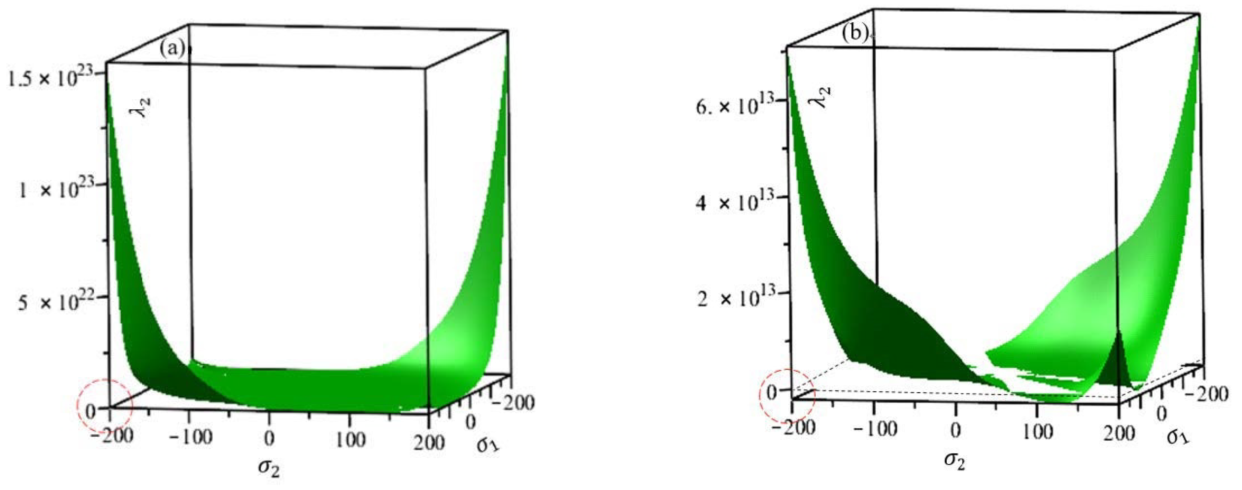
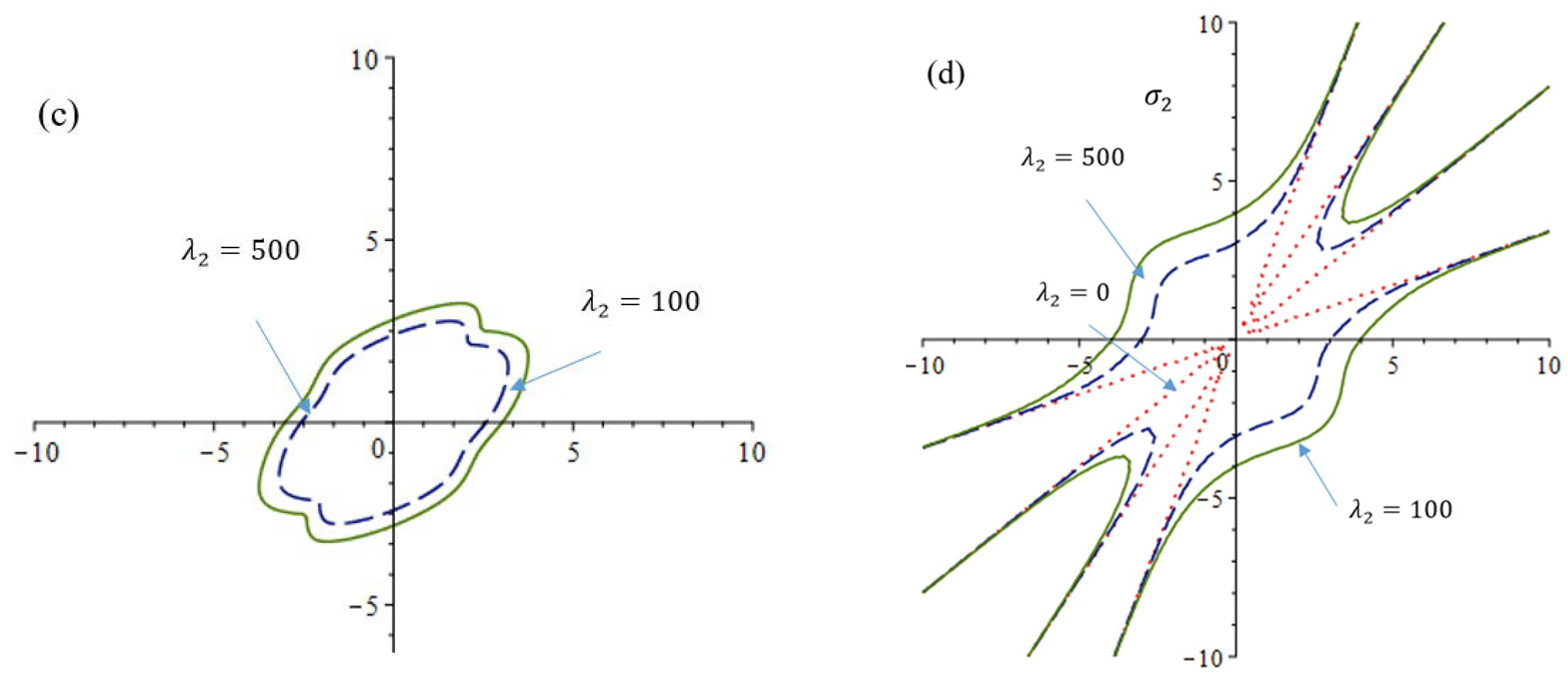
2.2. The Convexity Condition of the Yield Function

It is assumed that the yield surface is always convex because the internal plastic work must be dissipated during the plastic deformation of the material. This is called the convexity condition of the yield surface. In order to confirm the convexity of the yield condition for the proposed yield criterion in this study, the stress range in which the yield surface is convex was checked. For the isotropic yield function to be convex, the range of variation of α and β is α = 0 and β = [–4, 12]; β = 0 and α = [–12, 20]; α = (0, 3] and β = (0, 12]; α = [−6, 0) and β = [−4, 0); α = (0, 20] and β = [−4, 0); and α = [−12, 0) and β = (0, 12]. These results are for the case of a symmetric yield function with shear stress plane ${\sigma }_{xy}=0$.

The convexity of the proposed yield function is satisfied by confirming the convexities of $f\left({\sigma }_{xx}, {\sigma }_{yy}\right)$, $f\left({\sigma }_{xx}, {\sigma }_{xy}\right)$, and $f\left({\sigma }_{yy}, {\sigma }_{xy}\right)$. Mathematically, to ensure the convexity of each $f\left({\sigma }_i, {\sigma }_j\right)$ function, it is necessary to check whether the corresponding Hessian H is positive semidefinite [20,43,44]:

$$\begin{gathered} H_1\left({\mathsf{\sigma }}_{xx},{ \mathsf{\sigma }}_{yy}\right)=\frac{{\partial }^{2}f}{\partial {\sigma }_i\partial {\sigma }_j}=\left[\begin{array}{cc}\frac{{\partial }^{2}f}{\partial {\sigma }_{xx}^2}& \frac{{\partial }^{2}f}{\partial {\sigma }_{yy}\partial {\sigma }_{xx}}\\ \frac{{\partial }^{2}f}{\partial {\sigma }_{xx}\partial {\sigma }_{yy}}& \frac{{\partial }^{2}f}{\partial {\sigma }_{yy}^2}\end{array}\right] \\ {H}_2\left({\mathsf{\sigma }}_{xx},{ \mathsf{\sigma }}_{xy}\right)=\frac{{\partial }^{2}f}{\partial {\sigma }_i\partial {\sigma }_j}=\left[\begin{array}{cc}\frac{{\partial }^{2}f}{\partial {\sigma }_{xx}^2}& \frac{{\partial }^{2}f}{\partial {\sigma }_{xy}\partial {\sigma }_{xx}}\\ \frac{{\partial }^{2}g}{\partial {\sigma }_{xx}\partial {\sigma }_{xy}}& \frac{{\partial }^{2}g}{\partial {\sigma }_{xy}^2}\end{array}\right] \\ H_3\left({\mathsf{\sigma }}_{yy},{ \mathsf{\sigma }}_{xy}\right)=\frac{{\partial }^{2}f}{\partial {\sigma }_i\partial {\sigma }_j}=\left[\begin{array}{cc}\frac{{\partial }^{2}f}{\partial {\sigma }_{yy}^2}& \frac{{\partial }^{2}f}{\partial {\sigma }_{xy}\partial {\sigma }_{yy}}\\ \frac{{\partial }^{2}f}{\partial {\sigma }_{yy}\partial {\sigma }_{xy}}& \frac{{\partial }^{2}f}{\partial {\sigma }_{xy}^2}\end{array}\right] \end{gathered}$$

(25)

The positive semidefinite property of a Hessian matrix H can be proved by showing that the matrix eigenvalues are positive. Based on this analysis, it was confirmed that the yield function proposed in this study satisfies the convexity condition.

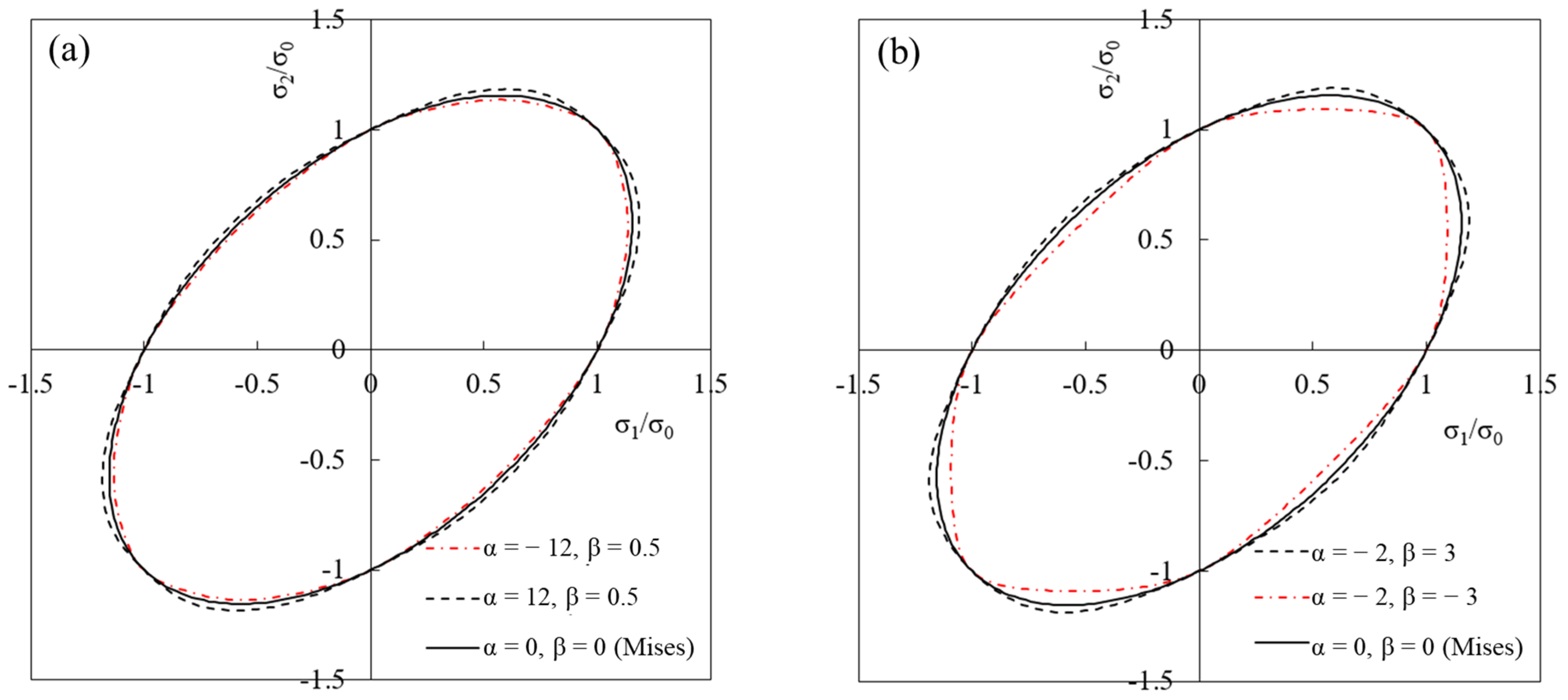
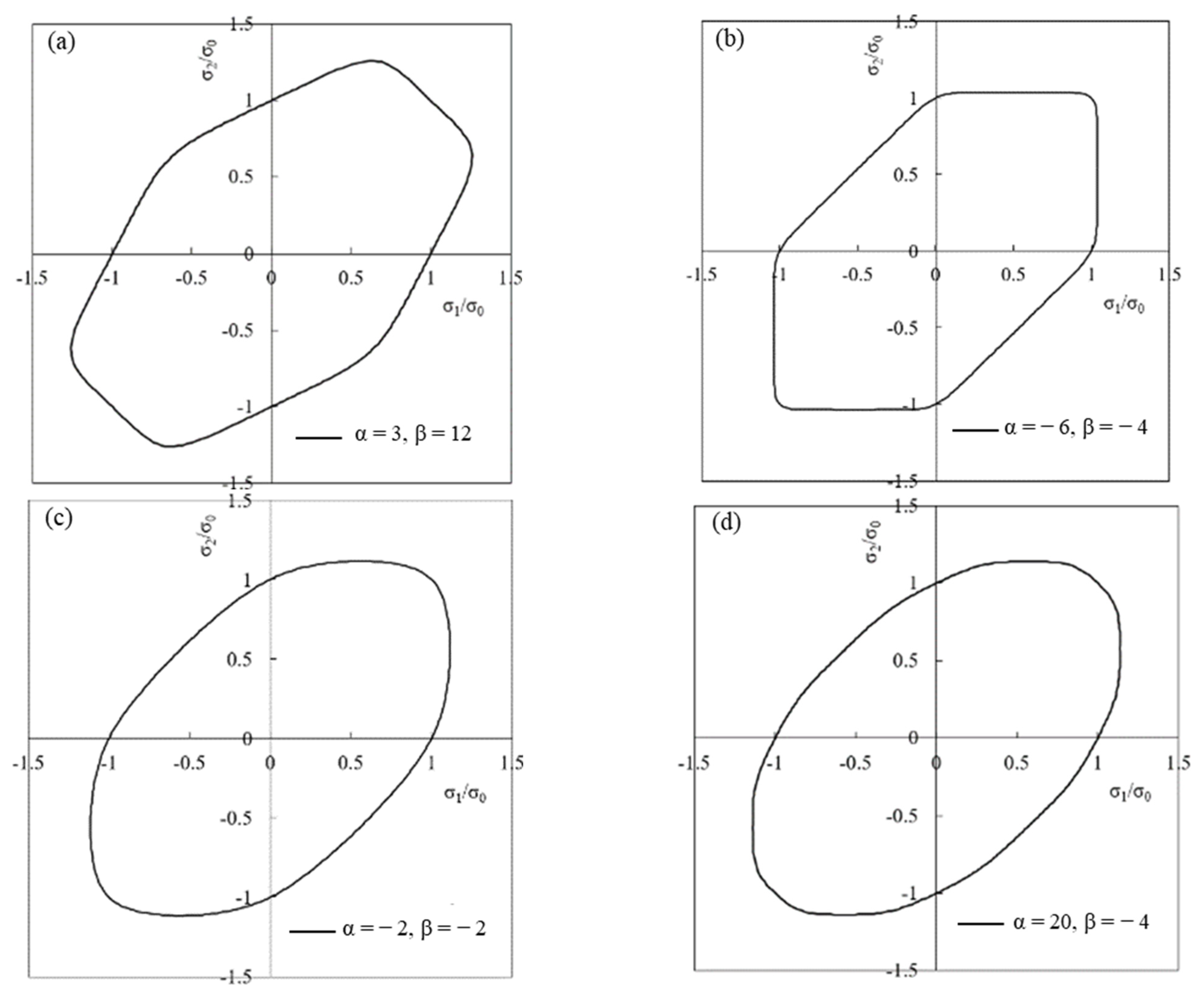
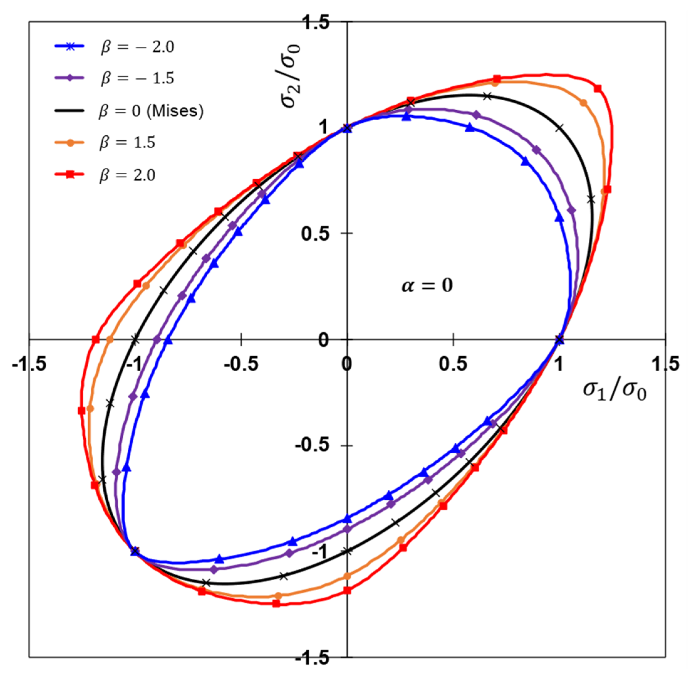
2.3. Effect of α and β on Yield Surface under Plane Stress

In order to confirm the role of the material parameters α and β of the proposed yield function in the isotropic form, $a_i=b_j=1$, various combinations of these parameters were adopted and the shape of the yield surface in the space of principal stresses under plane stress condition was observed. Figure 1 shows the predicted yield locus of Equation (17) for various combinations of α and β parameters to confirm the effect of each parameter. If both parameters α and β are 0, the proposed yield function returns to the Mises yield function. If α and β are both negative, the yield surface is inside the Mises yield surface, whereas if α and β are both positive, the yield surface is outside the Mises yield surface. Nevertheless, in both cases, the yield trajectory always passes through three points: (1, 0), (0, 1), and the equi-biaxial load (1, 1). When α is changed to α = −12 and α = 12, the shape of the yield surface does not change significantly (Figure 1a). In contrast, when β is changed to β = −3 and β = 3, the shape of the yield surface changes significantly (Figure 1b). That is, it can be seen that the parameter β affects the curvature of the yield surface more than α in the yield surface proposed in this study.

In addition, various combinations of the two parameters were reviewed to understand the flexibility of the proposed yield function. Figure 2 shows yield surfaces of different shapes according to parameters α and β. It can be seen that when α and β are negative numbers (α = −2 and β = −2), the curvature of the yield surface becomes smaller in the biaxial tensile region.

For the case of Equation (16), the asymmetric type of yield function, Figure 3 shows the effect of material parameter β with α = 0. The shape of the yield surface captures well the SD effect similar to Cazacu and Barlat (2004) and Khan et al. (2012) in that the yield stress in compression is larger than that in tension. Additionally note the asymmetric yield shape in that the proposed yield function reproduces the higher strength in equi-biaxial tension than in equi-biaxial compression observed in a titanium sheet of HCP crystal structure.

Therefore, it can be accepted that the yield function proposed in this study can express various types of yield surfaces by properly combining the two parameters α and β.

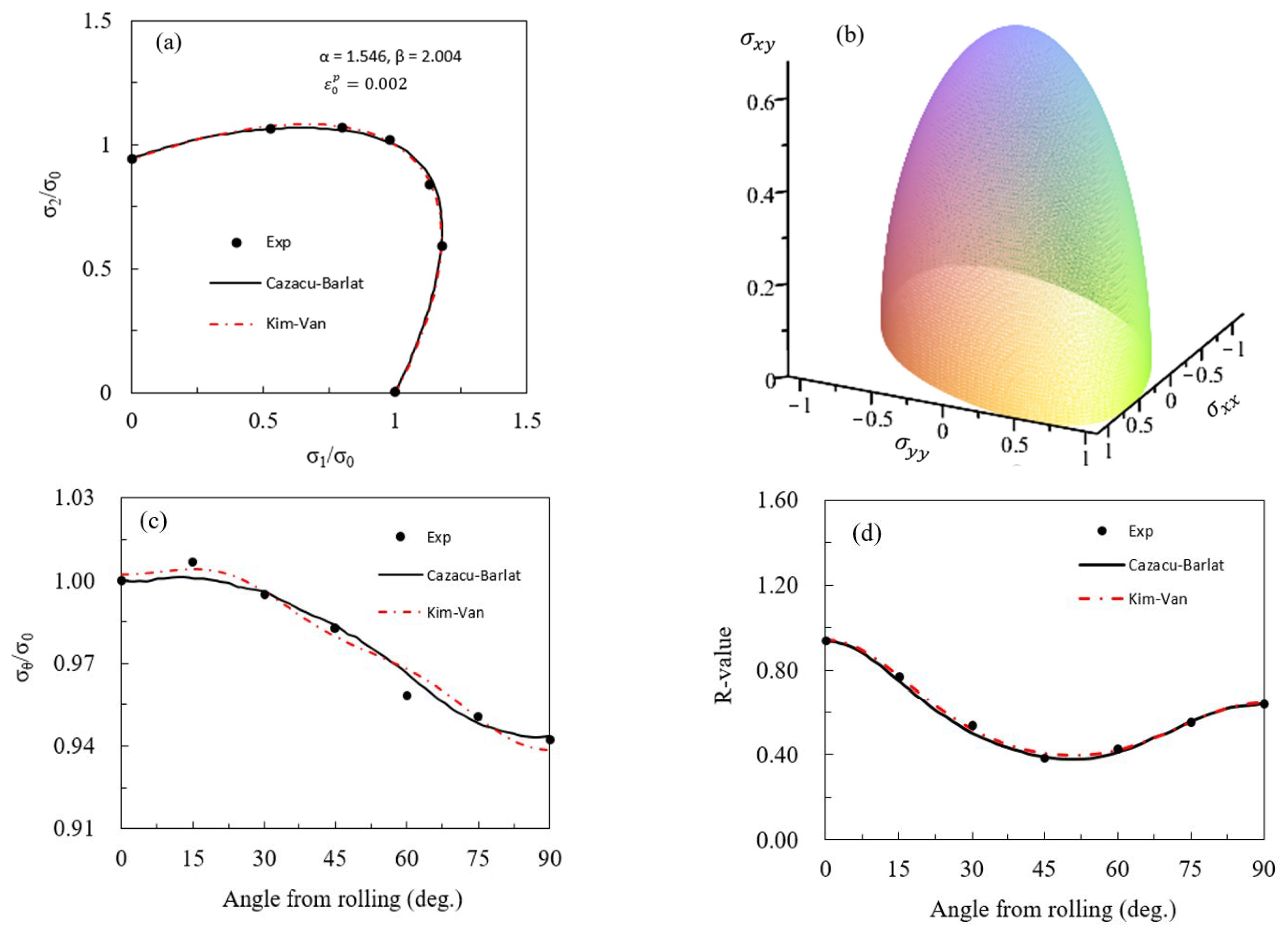
3. Application of the Proposed Yield Function Model

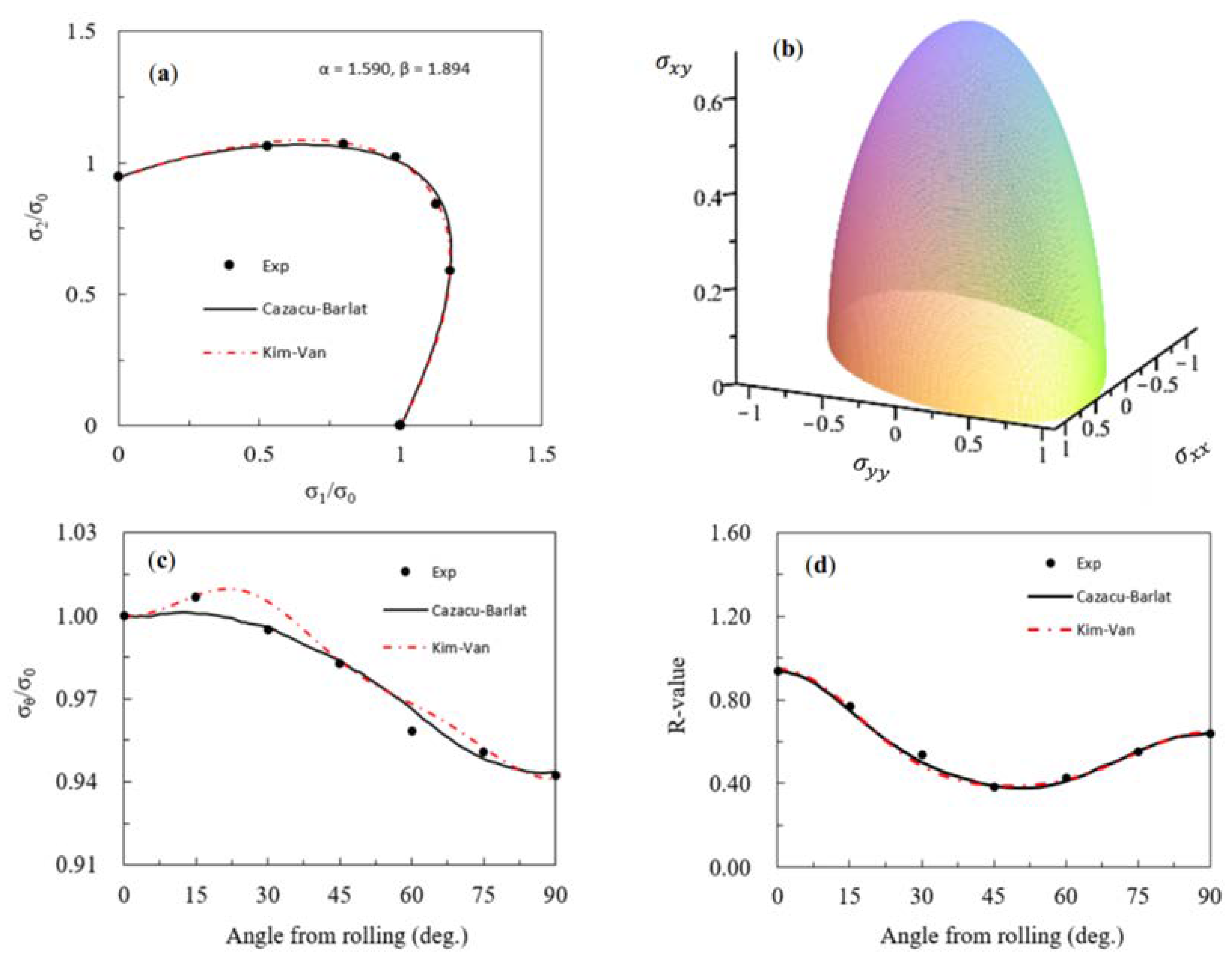
3.1. AA6016-T4 Sheet

In conventional methods used to determine parameters of the yield function, the uniaxial tension, pure shear, and hydraulic bulge test and biaxial tensile experiment with cruciform have been widely used [45]. In order to identify the parameters of the yield function developed by Cazacu-Barlat et al. (2001) for the AA6016-T4 sheet, the uniaxial tensile and hydraulic bulge test data were used [21,46,47].

In order to identify the parameters of the proposed yield function, the following error function was used to minimize the error value:

$$F={\sum }_i^n{\eta }_i{\left(1-\frac{{\left({\sigma }_{\theta }\right)}_i^{th}}{{\left({\sigma }_{\theta }\right)}_i^{data}}\right)}^2+{\sum }_j^m{\gamma }_j{\left(1-\frac{{\left(R_{\theta }\right)}_i^{th}}{{\left(R_{\theta }\right)}_i^{data}}\right)}^2+\delta {\left(1-\frac{{\left({\sigma }_b\right)}_i^{th}}{{\left({\sigma }_b\right)}_i^{data}}\right)}^2+v{\left(1-\frac{{\left(R_b\right)}_i^{th}}{{\left(R_b\right)}_i^{data}}\right)}^2+{\sum }_k^t{\chi }_k{\left(1-\frac{{\left(l\prime \right)}_k^{th}}{{\left(l\right)}_k^{data}}\right)}^2$$

(26)

Here, n and m represent the number of yield stress ${\sigma }_{\theta }$ and Lankford coefficient value $R_{\theta }$ in the direction obtained in the uniaxial tensile test, respectively. ${\sigma }_b$ and $R_b$ are the yield stress and Lankford coefficient of equi-biaxial tension, respectively. t denotes the amount of biaxial tension and compression tested at various load ratios, and the superscripts denotes whether each value is an experimental value (data) or a calculated value (th).

Additionally, ${\eta }_i,{\gamma }_i,\delta ,\nu$, and ${\chi }_k$ are weight factors for each term on the right side contributing to the error function. These weights are values arbitrarily determined by the user according to which factors are given priority to identify $a_i$ and $b_j$ because the experimental results in this study are greater than the number of equations [48,49,50]. Habraken et al. [49] set all of these weight factors to 1.0, and Nomura and Kuwabara [50] used the values that best fit the yield stress and anisotropy coefficient in the range of 1000~0.1. In this study, an appropriate value was used according to the problem so as not to fall into the local minimum value. ${\left(l\right)}_k^{data}$ and ${\left(l\prime \right)}_k^{th}$ are the distances between the origin and the experimental and predicted values in the principal stress space, respectively. That is, $l=$ $\sqrt{{\sigma }_1^2+{\sigma }_2^2}$.

Using KV’12S and the Cazacu–Barlat yield function (2001), the yield surface, normalized yield stress, and Lankford anisotropy coefficients for the AA6016-T4 sheet were predicted. Figure 4a,c,d are shown together with the experimental data. The coefficients used in the KV’12S yield function for in-plane stress ${\sigma }_3=0$ were identified using 16 experimental data of uniaxial tensions, i.e., the yield stresses and the Lankford coefficients at θ = 0°, 15°, 30°, 45°, 60°, 75°, and 90°, and the equiyield tension stress, i.e., equi-biaxial yield stress (${\sigma }_b/{\sigma }_0=1.0$ [21]) and the Lankford coefficient ($R_b$ = 1.05 [46]). These data were also used to minimize the error function, Equation (26). These coefficients are shown in

Table 1. Anisotropic coefficients of the Kim–Van and the Cazacu–Barlat yield functions (2001) for AA6016-T4 sheet (16 equations for fitting).

Parameters	a1	a2	a3	a4	b1	b2	b3	b4	b5	b10	α	β2	c	Error
Kim–Van	1.039	1.018	0.729	0.720	0.722	2.006	2.825	0.251	1.574	1.633	1.546	2.004	$\times$	0.0006
Cazacu–Barlat	0.334	0.815	0.815	0.420	0.040	−1.205	−0.958	0.306	0.153	−0.020	$\times$	$\times$	1.4	0.0007

.

Similarly, in the Cazacu–Barlat yield function, uniaxial tensile yield stress and Lankford modulus values tested in the directions θ = 0°, 30°, 45°, 75°, and 90° and biaxial tensile yield stress ${\sigma }_b/{\sigma }_0=1.0$ were used to identify the coefficients of the Cazacu–Barlat yield function. Figure 4a,c,d show the predicted yield surface, normalized yield stress, and Lankford coefficient values in the KV’12S model using the Cazacu–Barlat yield function, respectively. Figure 4b shows the shape of the yield surface considering the effect of shear stress on the KV’12S yield function.

From the results in Figure 4, the value of the Lankford coefficient according to the yield surface, normalized yield stress, and angle predicted by the KV’12S model had a low error value (i.e., F = 0.0006 for KV’12S and F = 0.0007 for the Cazacu–Barlat model), and it can be seen that the experimental results are well represented. However, the predicted uniaxial yield stress ${\sigma }_{\theta }/{\sigma }_0$ according to the angle was partially inconsistent with the corresponding experimental data at θ = 0°, 45°, and 90°. This is thought to be because overfitting occurred when 16 equations were used to fit the experimental data.

In order to prevent such overfitting at θ = 0°, 45°, and 90°, the anisotropy coefficients in the Kim–Van yield function were identified using a total of 12 experimental data, i.e., uniaxial tensile yield stress and Lankford values at θ = 0°, 15°, 45°, 75°, and 90°, and equi-biaxial tension, which were ${\sigma }_b/{\sigma }_0=1.0$ and $R_b$=1.05. The anisotropic coefficients identified are summarized in

Table 2. Anisotropic coefficients in the Kim–Van and the Cazacu–Barlat yield functions (2001) for AA6016-T4 sheet (12 equations for fitting).

Parameters	a1	a2	a3	a4	b1	b2	b3	b4	b5	b10	α	β2	c	Error
Kim–Van	1.020	1.035	0.787	0.685	0.747	1.871	2.744	0.296	1.720	1.656	1.590	1.894	$\times$	0.0013
Cazacu–Barlat	0.334	0.815	0.815	0.420	0.040	−1.205	−0.958	0.306	0.153	−0.020	$\times$	$\times$	1.4	0.0007

and the predictions are depicted in Figure 5.

In Figure 5, it can be seen that the predicted yield locus, surface, normalized yield stress, and Lankford coefficient values from the KV’12S yield function agreed well with the experiment at the angles taken to identify the parameters. However, the error value in this case (F = 0.0013) was larger than that of the Cazacu–Barlat model (F = 0.0007). The reason is incorrect predictions in the other data θ = 30° and 60°. Therefore, it can be concluded that it is necessary to take appropriate experimental data for each material to improve the prediction of material behavior.

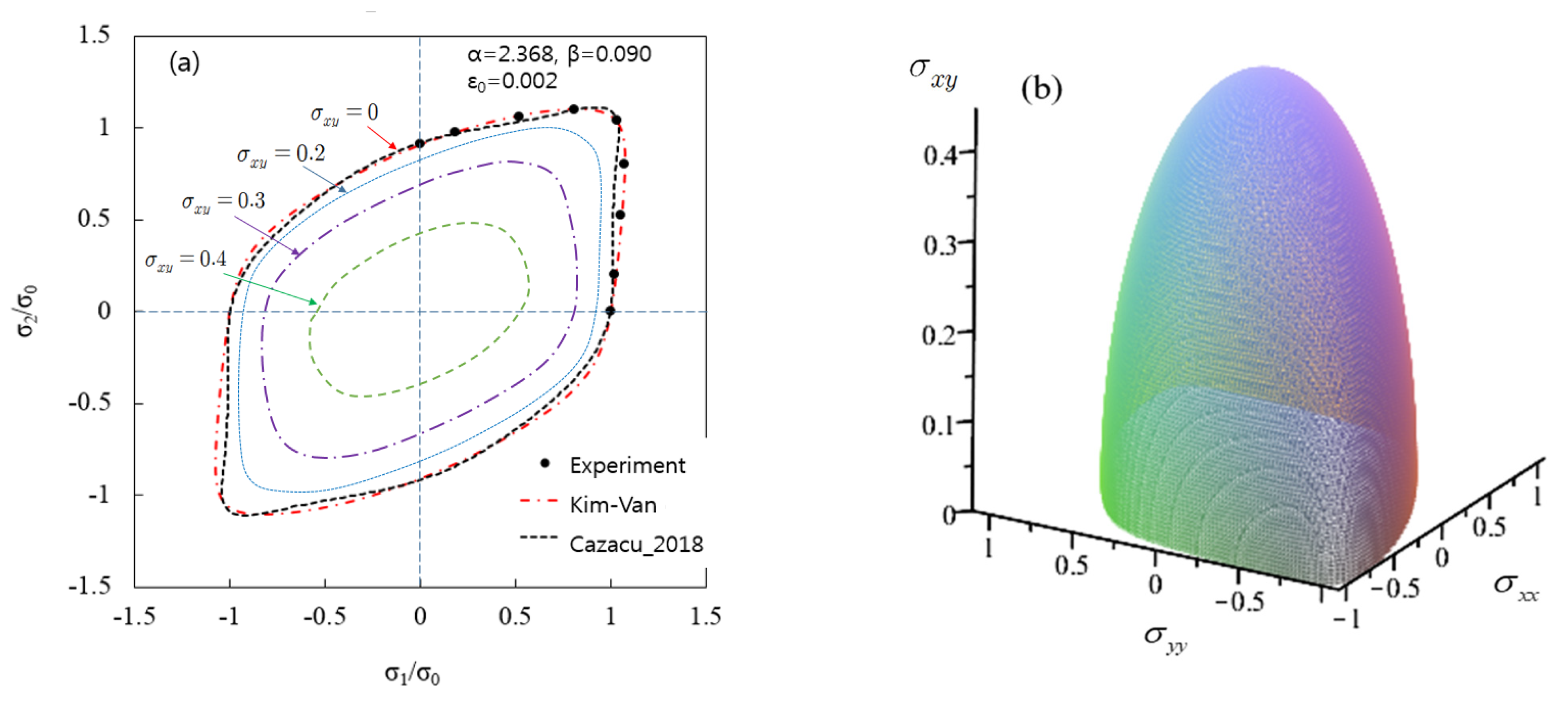
3.2. AA2090-Ts3 Sheet

In previous studies, in the case of the AA2090-T3 [51,52] sheet, the Yld2004-18p function was used to successfully describe the plastic anisotropy properties of strongly anisotropic materials. However, the Yld2004-18p yield function requires many experiments to identify parameters.

Here, to confirm the applicability of the KV’12S yield function to strongly anisotropic material, the predicted yield surface, normalized uniaxial yield stress, and Lankford coefficient for the AA2090-T3 sheet were compared with experimental results.

To identify the parameters of the KV’12S yield function, uniaxial tensile yield stress and Lankford modulus values according to θ = 0°, 15°, 45°, and 90°; biaxial tensile yield stress ${\sigma }_b/{\sigma }_0=1.035$; and biaxial yield stress values at three different load ratios of biaxial tension (i.e., ${\sigma }_x:{\sigma }_y=1:2, 4:3, 2:1$) were used. On the other hand, the coefficient of the Cazacu 2018 yield function (refer to Equation (7)) was identified by minimizing the error function (22) using the uniaxial tensile yield stress and Lankford coefficient value for θ = 0°, 30°, 45°, 75°, and 90° and biaxial yield stress ${\sigma }_b/{\sigma }_0=1.035$.

Table 3. Anisotropic coefficients of the Kim–Van and the Cazacu 2018 yield functions for AA2090-T3 sheet.

Parameters	a1	a2	a3	a4	b1	b2	b3	b4	b5	b10	α	β2	c	Error
Kim–Van	0.989	1.430	0.252	1.663	−0.544	−3.571	0.065	0.337	−2.049	−2.148	2.368	0.090	0.0837	0.0013
Cazacu–Barlat	0.779	1.596	1.427	1.813	2.009	0.255	−0.990	0.646	1.589	2.735	$-2.18$	$\times$	$\times$	0.0007

shows the coefficients of the two yield functions.

Figure 6a,c,d show the predicted yield surface, normalized yield stress, and Lankford coefficient values from the KV’12S and Cazacu 2018 yield functions together with experimental data. Figure 6a represents the yield locus with different shear stress ${\sigma }_{xy}/{\sigma }_0$ and shows clearly that the yield surfaces predicted by Equation (12) did not exhibit the same shape for different shear stresses; additionally, it shows couplings between shear and normal components of stress, as pointed in many crystal plasticity studies [53].

Moreover, the shape of the yield surface was quite sharp in equi-biaxial tension, and strong anisotropic behavior is shown in the Lankford coefficient value (Figure 6d). The prediction of the KV’12S yield function agreed well with the experiment. Error values were calculated to evaluate the predictability of material behavior for two yield functions. The error value of 0.0837 was calculated from the KV’12S yield function, while the Cazacu 2018 yield function could not be calculated. The reason is that the convexity of this yield function was not satisfied in the case of the Cazacu 2018 yield function as shown in the yield surface (Figure 6a).

To compare the difference in convexity between the two yield functions, a Hessian matrix (H) was observed. The first eigenvalue of a matrix H is always greater than or equal to the second eigenvalue. Therefore, only the second eigenvalue (${\lambda }_2$) was considered in this study.

In the case of the KV’12S yield function, it can be seen that the second eigenvalue of matrix H was always greater than or equal to 0 in the range of ${\sigma }_1=\left[-200, 200\right] \mathrm{MPa}$ and ${\sigma }_2=\left[-200, 200\right] \mathrm{MPa}$ (Figure 6a). On the other hand, the Cazacu 2018 yield function did not satisfy the convexity under some conditions (Figure 7b). In particular, in the range $\left({\sigma }_1,{\sigma }_2\right)=\left[200, 125\right] \mathrm{MPa}$ and $\left({\sigma }_1,{\sigma }_2\right)=\left[125, 200\right] \mathrm{MPa}$, the second-order eigenvalues were less than zero.

Figure 7c,d show the shape of the second invariant in the principal stress plane. The KV’12S yield function is a smooth shape without vertices as shown in Figure 7c. However, the Cazacu 2018 yield function as shown in Figure 7d has many protrusions. This phenomenon indicates that the yield curve predicted using the Cazacu 2018 model did not satisfy the convexity condition for the strongly anisotropic material. From this result, it can be concluded that the combination of the two parameters α and β in the KV’12S yield function proposed in this study can control the shape of the yield surface that satisfies the convexity of the strongly anisotropic material. In other words, the KV’12S yield function can control the various shapes of the yield surface in a wider range.

3.3. Pure Titanium Sheet

A commercially available pure titanium (CP-Ti) sheet having an HCP crystal structure exhibited an asymmetric shape in the yield curve. To explain the asymmetric plastic yield behavior of CP-Ti materials, Yoon et al. [42] proposed a new yield function having a coupling effect of all three stress invariants as shown in Equation (10). To describe the SD effect of the yield stress difference appearing in tension and compression tests, we adopted the KV’12A yield function, and the anisotropic parameters were determined from the experimental results of uniaxial tension and compression tests and equi-biaxial tension and compression tests.

Figure 8 shows experimental data from [42] and the Yoon 2014 yield function together to confirm the applicability of the KV’12A asymmetric yield function of Equation (12) for HCP material.

To identify the parameters of the KV’12A yield function, biaxial tension and compression data for three stress ratios (1:0, 1:1, 0:1) and the predicted data from the yield function of Yoon 2014 for three stress ratios (2:1, 3:4, 1:2) were used to minimize the error function, Equation (26). The derived parameters are shown in

Table 4. Anisotropic coefficients of the Kim–Van yield function for high-purity α-titanium sheet.

Parameters	a1	a2	a3	a4	b1	b2	b3	b4	b5	b10	α	β2	c	Error
Kim–Van	1.014	0.673	0.660	x	1.159	1.765	1.063	1.089	x	x	1.124	1.654	$\times$	0.0007

.

The yield locus predicted by the KV’12A and Yoon 2014 yield function showed a slight difference under the equi-biaxial tension and the compression modes, but the result predicted from KV’12A was in good agreement with the experimental results overall.

Therefore, it can be concluded that the anisotropic yield function of Kim–Van proposed in this study predicted not only the symmetrical yield behavior in BCC and FCC crystal structures well, but also the asymmetric yield behavior in HCP crystal structures.

4. Conclusions

In this study, a new anisotropic yield function expressed as $J_2$ and $J_3$ invariants including two parameters α and β and are proposed so that the plastic anisotropy behavior of the sheet can be well described. This yield function has been proposed to express two types of yield surfaces well: the symmetrical yield surface in BCC and FCC crystalline materials and the asymmetrical yield surface in HCP crystalline materials.

To confirm the validity of the proposed yield function, the plastic properties of the AA2090-T4 sheet with strong anisotropic material behavior as the symmetric yield function (KV’12S) and commercial pure titanium sheet as the asymmetric yield function (KV’12A) were predicted and compared with the existing anisotropic yield functions. The following main conclusions were drawn from this study:

(1)

The KV’12S yield function results in the Von Mises yield function when the two parameters α and β are zero.

(2)

KV’12S can also well represent various types of yield curves including strongly anisotropic materials. It was shown that the proposed yield function can implement various types of yield surface shapes by combining the two parameters α and β.

(3)

To verify the flexibility of the proposed model, the convexity of the yield surface was checked and compared with the Cazacu 2018 yield function. The convexity of KV’12S was satisfied in most stress ranges, but the Cazacu 2018 yield function for the material covered in this study did not satisfy the convexity in some stress ranges.

(4)

As a result of applying the KV’12S yield function proposed in this study to the AA2090-T4 material, which exhibited very strong anisotropy, the results deviated from some experimental data. Attention should be paid to the selection of experimental data used for the parameter optimization of the yield function proposed in this study. In this case, twelve experimental data (e.g., ten experimental data from the uniaxial tensile test and two experimental data from the equi-biaxial tension test) are recommended.

(5)

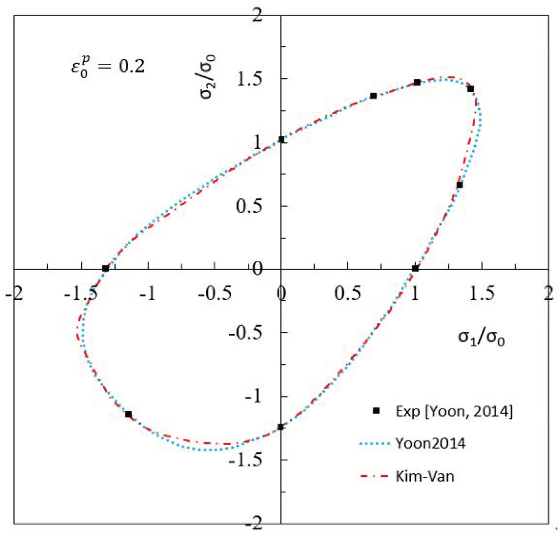
The KV’21A yield function was used to predict the yield surface of a commercial pure titanium sheet that exhibited an asymmetrical yield surface shape, and it was compared with the Yoon 2014 yield function and experimental data. Both yield functions were in good agreement with the experiment overall.

In a future study, the anisotropic yield function proposed in this study will be applied to the forming limit curve prediction. In addition, the effectiveness of the proposed yield function is evaluated by applying it to the finite element analysis of the sheet material processing process such as the cup drawing process and the incremental sheet forming process.

References

1. Zhan, M.; Guo, K.; Yang, H. Advances and trends in plastic forming technologies for welded tubes. Chin. J. Aeronaut. 2016, 29, 305–315. [Google Scholar] [CrossRef] [Green Version]
2. Meng, B.; Wan, M.; Wu, X.; Yuan, S.; Xu, X.; Liu, J. Inner wrinkling control in hydrodynamic deep drawing of an irregular surface part using drawbeads. Chin. J. Aeronaut. 2014, 27, 697–707. [Google Scholar] [CrossRef] [Green Version]
3. Li, X.; Song, N.; Guo, G.; Sun, Z. Prediction of forming limit curve (FLC) for Al–Li alloy 2198-T3 sheet using different yield functions. Chin. J. Aeronaut. 2013, 26, 1317–1323. [Google Scholar] [CrossRef] [Green Version]
4. Swift, H. Plastic instability under plane stress. J. Mech. Phys. Solids 1952, 1, 1–18. [Google Scholar] [CrossRef]
5. Voce, E. The relationship between stress and strain for homogeneous deformation. J. Inst. Met. 1948, 74, 537–562. [Google Scholar]
6. Pham, Q.T.; Oh, S.H.; Kim, Y.S. An efficient method to estimate the post-necking behavior of sheet metals. Int. J. Adv. Manuf. Technol. 2018, 98, 2563–2578. [Google Scholar] [CrossRef]
7. Stoughton, T.B.; Yoon, J.W. On the existence of indeterminate solutions to the equations of motion under non-associated flow. Int. J. Plast. 2008, 24, 583–613. [Google Scholar] [CrossRef]
8. Stoughton, T.B.; Yoon, J.W. Anisotropic hardening and non-associated flow in proportional loading of sheet metals. Int. J. Plast. 2009, 25, 1777–1817. [Google Scholar] [CrossRef]
9. Ha, J.J.; Coppieters, S.; Korkolis, Y.P. On the expansion of a circular hole in an orthotropic elastoplastic thin sheet. Int. J. Mech. Sci. 2020, 182, 105706. [Google Scholar] [CrossRef]
10. Pham, Q.T.; Kim, Y.S. Identification of the plastic deformation characteristics of AL5052-O sheet based on the non-associated flow rule. Met. Mater. Int. 2017, 23, 254–263. [Google Scholar] [CrossRef]
11. Kim, J.J.; Pham, Q.T.; Kim, Y.S. Thinning prediction of hole-expansion test for DP980 sheet based on a non-associated flow rule. Int. J. Mech. Sci. 2021, 191, 106067. [Google Scholar] [CrossRef]
12. Wu, B.; Ito, K.; Mori, N.; Oya, T.; Taylor, T.; Yanagimoto, J. Constitutive equations based on non-associated flow rule for the analysis of forming of anisotropic sheet metals. Int. J. Precis. Eng. Manuf. Green Technol. 2019, 7, 465–480. [Google Scholar] [CrossRef]
13. Prager, W. Recent developments in the mathematical theory of plasticity. J. App. Phys. 1949, 20, 235–241. [Google Scholar] [CrossRef]
14. Tresca, H. Mémoire sur l’écoulement des corps solides soumis à de fortes pressions. CR Acad. Sci. Paris 1864, 59, 754–758. [Google Scholar]
15. Mises, V. Mechanics of solid bodies in the plastically-deformable state. Math. Phys. 1913, 4, 582–592. [Google Scholar]
16. Drucker, D.C. Relations of experiments to mathematical theories of plasticity. J. Appl. Mech. 1949, 16, 349–357. [Google Scholar] [CrossRef]
17. Hill, R. A theory of the yielding and plastic flow of anisotropic metals. Proc. R. Soc. Lond. A 1948, 193, 281–297. [Google Scholar]
18. Hill, R. Theoretical plasticity of textured aggregates. Math. Proc. Camb. Phil. Soc. 1979, 85, 179–191. [Google Scholar] [CrossRef]
19. Hosford, W.F. On yield loci of anisotropic cubic metals. In Proceedings of the 7th North American Metalworking Conference, SME, Dearborn, MI, USA, 13–16 May 1979; pp. 191–197. [Google Scholar]
20. Barlat, F.; Brem, J.C.; Yoon, J.W.; Chung, K.; Dick, R.E.; Lege, D.J.; Pourboghrat, F.; Choi, S.-H.; Chu, E. Plane stress yield function for aluminum alloy sheets—Part 1: Theory. Int. J. Plast. 2003, 19, 1297–1319. [Google Scholar] [CrossRef]
21. Cazacu, O.; Barlat, F. Generalization of Drucker’s yield criterion to orthotropy. Math. Mech. Solids 2001, 6, 613–630. [Google Scholar] [CrossRef]
22. Barlat, F.; Aretz, H.; Yoon, J.W.; Karabin, M.E.; Brem, J.C.; Dick, R.E. Linear transformation based anisotropic yield function. Int. J. Plast. 2005, 21, 1009–1039. [Google Scholar] [CrossRef]
23. Banabic, D. Sheet Metal Forming Processes: Constitutive Modelling and Numerical Simulation; Springer: Heidelberg, Germany; Dordrecht, The Netherlands; London, UK; New York, NY, USA, 2010. [Google Scholar]
24. Banabic, D.; Barlat, F.; Cazacu, O.; Kuwabara, T. Advances in anisotropic behaviour and formability of sheet metals. Int. J. Mater. Form. 2020, 13, 749–787. [Google Scholar] [CrossRef]
25. Yoshida, F.; Hamasaki, H.; Uemori, T. A user-friendly 3D yield function to describe anisotropy of steel sheet. Int. J. Plast. 2013, 45, 119–139. [Google Scholar] [CrossRef]
26. Lou, Y.S.; Yoon, J.W. J2-J3 based anisotropic yield function under spatial loading. Procedia Eng. 2017, 207, 233–238. [Google Scholar] [CrossRef]
27. Karafillis, A.P.; Boyce, M.C. A general anisotropic yield criterion using bounds and a transformation weighting tensor. J. Mech. Phys. Solids 1993, 41, 1859–1886. [Google Scholar] [CrossRef]
28. Cazacu, O. New yield criteria for isotropic and textured metallic materials. Int. J. Solids Struct. 2018, 139–140, 200–210. [Google Scholar] [CrossRef]
29. Kabirian, F.; Khan, A.S. Anisotropic yield criteria in σ-τ stress space for materials with yield asymmetry. Int. J. Solids Struct. 2015, 67, 116–126. [Google Scholar] [CrossRef]
30. Koh, Y.; Kim, D.; Seok, D.Y.; Bak, J.; Kim, S.W.; Lee, Y.S.; Chung, K. Characterization of mechanical property of magnesium AZ31 alloy sheets for warm temperature forming. Int. J. Mech. Sci. 2015, 93, 204–217. [Google Scholar] [CrossRef]
31. Chandola, N.; Lebensohn, R.A.; Cazacu, O.; Revil-Baudard, B.; Mishra, R.K.; Barlat, F. Combined effects of anisotropy and tension–compression asymmetry on the torsional response of AZ31 Mg. Int. J. Solids Struct. 2015, 58, 190–200. [Google Scholar] [CrossRef]
32. Tari, G.; Worswick, M.J. Elevated temperature constitutive behavior and simulation of warm forming of AZ31BD. J. Mater. Process. Technol. 2015, 221, 40–55. [Google Scholar] [CrossRef]
33. Tari, D.G.; Worswick, M.J.; Alia, U.; Gharghourib, M.A. Mechanical response of AZ31B magnesium alloy: Experimental characterization and material modeling considering proportional loading at room temperature. Int. J. Plast. 2014, 55, 247–267. [Google Scholar] [CrossRef]
34. Muhammad, W.; Mohammadi, M.; Kang, J.; Mishra, R.K.; Inal, K. An elasto-plastic constitutive model for evolving asymmetric/anisotropic hardening behavior of AZ31B and ZEK100 magnesium alloy sheets considering monotonic and reverse loading paths. Int. J. Plast. 2015, 70, 30–59. [Google Scholar] [CrossRef]
35. Khan, A.S.; Pandey, A.; Gnäupel-Herold, T.; Mishra, R.K. Mechanical response and texture evolution of AZ31 alloy at large strains for different strain rates and temperatures. Int. J. Plast. 2011, 27, 688–706. [Google Scholar] [CrossRef]
36. Liu, C.; Huang, Y.; Stout, M.G. On the asymmetric yield surface of plastically orthotropic materials: A phenomenological study. Acta Mater. 1997, 45, 2397–2406. [Google Scholar] [CrossRef]
37. Shimizu, I.; Tada, N. Plastic behavior of polycrystalline aluminum during biaxial compression with strain path change. Key Eng. Mater. 2007, 340, 883–888. [Google Scholar]
38. Cazacu, O.; Barlat, F. A criterion for description of anisotropy and yield differential effects in pressure-insensitive metals. Int. J. Plast. 2004, 20, 2027–2045. [Google Scholar] [CrossRef]
39. Cazacu, O.; Plunkett, B.; Barlat, F. Orthotropic yield criterion for hexagonal closed packed metals. Int. J. Plast. 2006, 22, 1171–1194. [Google Scholar] [CrossRef]
40. Gao, X.; Zhang, T.; Zhou, J.; Graham, S.M.; Hayden, M.; Roe, C. On stress-state dependent plasticity modeling: Significance of the hydrostatic stress, the third invariant of stress deviator and the non-associated flow rule. Int. J. Plast. 2011, 27, 217–231. [Google Scholar] [CrossRef]
41. Khan, A.S.; Yu, S.; Liu, H. Deformation induced anisotropic responses of Ti–6Al–4V alloy Part II: A strain rate and temperature dependent anisotropic yield criterion. Int. J. Plast. 2012, 38, 14–26. [Google Scholar] [CrossRef]
42. Yoon, J.W.; Lou, Y.; Yoon, J.; Glazoff, M.V. Asymmetric yield function based on the stress invariants for pressure sensitive metals. Int. J. Plast. 2014, 56, 184–202. [Google Scholar] [CrossRef]
43. Cardoso, R.P.R.; Adetoro, O.B. A generalisation of the Hill’s quadratic yield function for planar plastic anisotropy to consider loading direction. Int. J. Mech. Sci. 2017, 128–129, 253–268. [Google Scholar] [CrossRef]
44. Laydi, M.R.; Lexcellent, C. Yield criteria for shape memory materials: Convexity conditions and surface transport. Math. Mech. Solids 2010, 15, 165–208. [Google Scholar] [CrossRef]
45. Zhang, S.; Leotoing, L.; Guines, D.; Thuillier, S.; Zang, S.L. Calibration of anisotropic yield criterion with conventional tests or biaxial test. Int. J. Mech. Sci. 2014, 85, 142–151. [Google Scholar] [CrossRef] [Green Version]
46. Lăzărescu, L.; Nicodim, I.; Ciobanu, I.; Comşa, D.S.; Banabic, D. Determination of material parameters of sheet metals using the hydraulic bulge test. Acta Metall. Slovaca 2013, 19, 4–12. [Google Scholar] [CrossRef] [Green Version]
47. Tamura, S.; Sumikawa, S.; Uemori, T.; Hamasaki, H.; Yoshida, F. Experimental observation of elasto-plasticity behavior of type 5000 and 6000 aluminum alloy sheets. Mater. Trans. 2011, 52, 868–875. [Google Scholar] [CrossRef]
48. Sarraf, I.S.; Green, D.E. Prediction of DP600 and TRIP780 yield loci using Yoshida anisotropic yield function. IOP Conf. Ser. Mater. Sci. Eng. 2018, 418, 012089. [Google Scholar] [CrossRef] [Green Version]
49. Habraken, A.M.; Aksen, T.A.; Alves, J.L.; Amaral, R.L.; Betaieb, E.; Chandola, N.; Corallo, L.; Cruz, D.J.; Duchêne, L.; Engel, B.; et al. Analysis of ESAFORM 2021 cup drawing benchmark of an Al alloy, critical factors for accuracy and efficiency of FE simulations. Int. J. Mater. Form. 2022, 15, 61. [Google Scholar] [CrossRef]
50. Nomura, S.; Kuwabara, T. Material modeling of hot-rolled steel sheet considering differential hardening and hole expansion simulation. ISIJ Int. 2022, 62, 191–199. [Google Scholar] [CrossRef]
51. Yoon, J.W.; Barlat, F.; Dick, R.E.; Karabin, M.E. Prediction of six or eight ears in a drawn cup based on a new anisotropic yield function. Int. J. Plast. 2006, 22, 174–193. [Google Scholar] [CrossRef]
52. Tang, B.; Wang, Z.; Guo, N.; Wang, Q.; Liu, P. An Extended Drucker Yield Criterion to Consider Tension–Compression Asymmetry and Anisotropy on Metallic Materials: Modeling and Verification. Metals 2020, 10, 20. [Google Scholar] [CrossRef]
53. Piehler, H.R. Crystal-plasticity fundamentals. ASM Handb. 2009, 22, 232. [Google Scholar]
Figure 1. Yield locus according to proposed isotropic yield function for different values of parameters α and β: (a) effect of parameter α, and (b) effect of parameter β.
Metals 13 00142 g001
Figure 2. General yield loci shapes obtained using the isotropic yield: (a) α = 3, β = 12; (b) α = −6, β = −4; (c) α = −2, β = −2; (d) α = 20, β = −4.
Metals 13 00142 g002
Figure 3. General yield loci predicted by the proposed isotropic yield function for α = 0; β =−2.0~2.0.
Metals 13 00142 g003
Figure 4. Predicted anisotropy according to the Kim–Van and the Cazacu–Barlat yield functions (2001) for AA6016-T4 sheet with 16 equations for fitting (a) yield locus, (b) 3D yield surface, (c) normalized uniaxial yield stresses, and (d) R-values.
Metals 13 00142 g004
Figure 5. Predicted anisotropy according to the Kim–Van and the Cazacu–Barlat yield functions (2001) for AA6016-T4 sheet with 12 equations for fitting (a) yield locus, (b) 3D yield surface, (c) normalized uniaxial yield stresses, and (d) R-values.
Metals 13 00142 g005
Figure 6. Predicted anisotropy according to the Kim–Van and the Cazacu 2018 yield functions for AA2090-T3 sheet with 12 equations for fitting (a) yield locus, (b) 3D yield surface, (c) normalized uniaxial yield stresses, and (d) R-values.
Metals 13 00142 g006aMetals 13 00142 g006b
Figure 7. Calculated second eigenvalue (λ2) of Hessian matrix at σ 12 = 0 for AA2090-T3 sheet: (a) Kim–Van yield function; (b) Cazacu 2018 yield function; (c) contour lines of eigenvalue of Kim–Van model; (d) contour lines of eigenvalue of Cazacu 2018 model.
Metals 13 00142 g007aMetals 13 00142 g007b
Figure 8. Yield loci of high-purity α-titanium sheet predicted using the Kim–Van and the Yoon 2014 yield functions.
Metals 13 00142 g008