Review

Understanding the Mechanism of Abrasive-Based Finishing Processes Using Mathematical Modeling and Numerical Simulation

1
Advanced Manufacturing and Mechatronics Lab, Department of Mechanical Engineering, Malaviya National Institute of Technology, Jaipur 302017, India
2
Department of Mechanical Engineering, GLA University, Mathura 281406, India
3
Department of Mechanical Engineering and Industrial Design, University of Cadiz, 11003 Cadiz, Spain
4
School of Mechanical Engineering, Lovely Professional University, Phagwara 144001, India
5
Division of Research & Innovation, Uttaranchal University, Dehradun 248007, India
6
Department of Mechanical Engineering, University of Aveiro, Campus Santiago, 3810-193 Aveiro, Portugal
7
Department of Medical Physics, Hilla University College, Babylon 51002, Iraq
*
Author to whom correspondence should be addressed.
Metals 2022, 12(8), 1328; https://doi.org/10.3390/met12081328
Submission received: 12 June 2022 / Revised: 1 August 2022 / Accepted: 1 August 2022 / Published: 8 August 2022
(This article belongs to the Special Issue Machining and Finishing Processes for Metals)

Abstract

:
Recent advances in technology and refinement of available computational resources paved the way for the extensive use of computers to model and simulate complex real-world problems difficult to solve analytically. The appeal of simulations lies in the ability to predict the significance of a change to the system under study. The simulated results can be of great benefit in predicting various behaviors, such as the wind pattern in a particular region, the ability of a material to withstand a dynamic load, or even the behavior of a workpiece under a particular type of machining. This paper deals with the mathematical modeling and simulation techniques used in abrasive-based machining processes such as abrasive flow machining (AFM), magnetic-based finishing processes, i.e., magnetic abrasive finishing (MAF) process, magnetorheological finishing (MRF) process, and ball-end type magnetorheological finishing process (BEMRF). The paper also aims to highlight the advances and obstacles associated with these techniques and their applications in flow machining. This study contributes the better understanding by examining the available modeling and simulation techniques such as Molecular Dynamic Simulation (MDS), Computational Fluid Dynamics (CFD), Finite Element Method (FEM), Discrete Element Method (DEM), Multivariable Regression Analysis (MVRA), Artificial Neural Network (ANN), Response Surface Analysis (RSA), Stochastic Modeling and Simulation by Data Dependent System (DDS). Among these methods, CFD and FEM can be performed with the available commercial software, while DEM and MDS performed using the computer programming-based platform, i.e., “LAMMPS Molecular Dynamics Simulator,” or C, C++, or Python programming, and these methods seem more promising techniques for modeling and simulation of loose abrasive-based machining processes. The other four methods (MVRA, ANN, RSA, and DDS) are experimental and based on statistical approaches that can be used for mathematical modeling of loose abrasive-based machining processes. Additionally, it suggests areas for further investigation and offers a priceless bibliography of earlier studies on the modeling and simulation techniques for abrasive-based machining processes. Researchers studying mathematical modeling of various micro- and nanofinishing techniques for different applications may find this review article to be of great help.

1. Introduction

Metal cutting is considered the most significant procedure where the material removal process is performed by more than one edge to fulfill some of the specific criteria needed to shape the final workpiece in the form of particular geometrical dimensions and surface finish. Even though there has occurred a lot of advancement in the development of machining tools and process controlling and monitoring, there still exists room for improvement in metal cutting processes and procedures for which significant research can be conducted by various metal-forming industries [1]. This may occur due to the optimizing procedures’ intricacy, particularly when the materials with higher “mechanical characteristics” are developed and the machinability has not yet been inspected fully [2].
In addition to the material removal and metal cutting process, there is a fine requirement that product surface quality is considerably better since they play a major role in aerospace, automotive, and biomedical industries [3]. Even a small scratch or an uneven burr can cause huge damage to the engine. It may fail the aerospace gadgets or malfunction any of its components, etc. These industries are trying their best to spend a huge amount on the finishing of such components in order to make components that are cutting/burrs marks-free [4]. For the last 40 years, various manufacturing industries have been using conventional procedures for finishing the components, such as grinding, honing, lapping, etc., to get the machining components’ desired finishing. However, these conventional procedures of finishing are restricted to very few geometries and cannot work on complex and intricate geometries as well as complicated profiles for finishing of high level, which is required while the operation of the component is in process. These limitations and restrictions in the finishing process have led the industries to develop advanced finishing procedures, known as “Abrasive flow machining (AFM)” [5]. AFM process is used to perform the finishing process of the machining components and its internal features in several engineering materials such as alloys, ceramics, non-ferrous, super-alloys, refractory materials, semiconductors, carbides, quartz, and various other composites, etc., that are considered to be difficult to be done using the traditional processes economically and proficiently [6]. The significance of this AFM process is that it generates the nano-level finishing of the machining components that are essentially desirable at this time. The concept of the AFM finishing procedure was first given by the “Extrude Hone corporation of the USA” in 1960 for the finishing of aerospace components to achieve the desired accuracy. These days, the AFM process is the best technique for finishing intricate geometries, which were never achievable by any traditional finishing tools. Even a lot of study has been conducted by researchers in order to improve the finishing process performed by the AFM [7]. The AFM process efficiently improves the surface finish of the complicated geometry like gears, trim-dies, turbine blades, bio-medical implants, etc. [8,9]. Many researchers have highlighted the potential of the AFM process to finish any complex and freeform surfaces [10,11]. Researchers have also developed a hybrid form of AFM processes, i.e., rotational type abrasive flow machining (R-AFM), to finish the asymmetrical complicated workpiece [12]. Magnetorheological abrasive flow finishing (MRAFF) has also been developed under the umbrella of the hybrid AFM process to finish optical surfaces [13]. Many researchers have employed the AFM and its hybrid variants for surface finishing of metal matrix composite materials, i.e., Al/SiC MMCs [14,15]. Hybrid manufacturing processes, i.e., ultrasonic-assisted machining processes, are also a good solution due to less cutting force required during the machining operation [16]. Ultrasonic-assisted magnetic abrasive finishing (UAMAF) significantly improves the surface roughness as well as the hardness of the workpiece [17,18]. Centrifugal force-assisted abrasive flow machining (CFAFM) is an efficient hybrid machining process to finish cylindrical surfaces with better surface roughness [19].

1.1. An Overview of Abrasive-Based Machining Processes and Their Types

1.1.1. Loose Abrasive-Based Machining Processes

The loose AFM process is considered the most significant approach to finishing the intricate and complex geometries and advanced materials used within industrial practices [20,21]. It is considered to be the recently developed “surface finishing process” that has been used widely in various industrial applications such as defense, aerospace, bio-medical, tool and die, etc. [22]. In loose AFM, no structure exists that connects or links the grains together in the matrix in bonded “abrasive process.” The various standard processes in Loose abrasive processes include AFM, polishing, lapping honing, and abrasive blasting. AFM is also one of the finishing techniques that entail the oil for the particle of abrasive and carrier polymer and assists in eliminating the barriers to acquiring the desired size and shape [14]. Thus, any complicated shape can be easily finished by Abrasive Flow Machining abbreviated AFM. Abrasive flow machining helped us to tackle the shortcomings of conventional processes like “grinding,” “lapping,” and “honing” [20]. The problem associated with AFM is its high cost and “low material removal rate MRR,” which makes it laborious and strenuous. AFM processes of finishing techniques have also emerged recently to tackle the challenges and issues such as processes requiring high machining time [23,24,25,26]. Figure 1 below illustrates the “loose abrasive-based machining” (LAM) process.
Figure 2 below signifies the various categories and sub-categories of the loose abrasive-based machining process.
The machining accuracy of different traditional and advanced machining processes is described in Figure 3.
A summary of loose abrasive-based machining processes about their basic principle and process parameters is shown in Table 1.
The comparison of surface roughness of traditional finishing techniques s shown in Figure 4 below.
The comparison of surface roughness of advanced finishing techniques, i.e., nano finishing techniques, is shown in Figure 5 below.

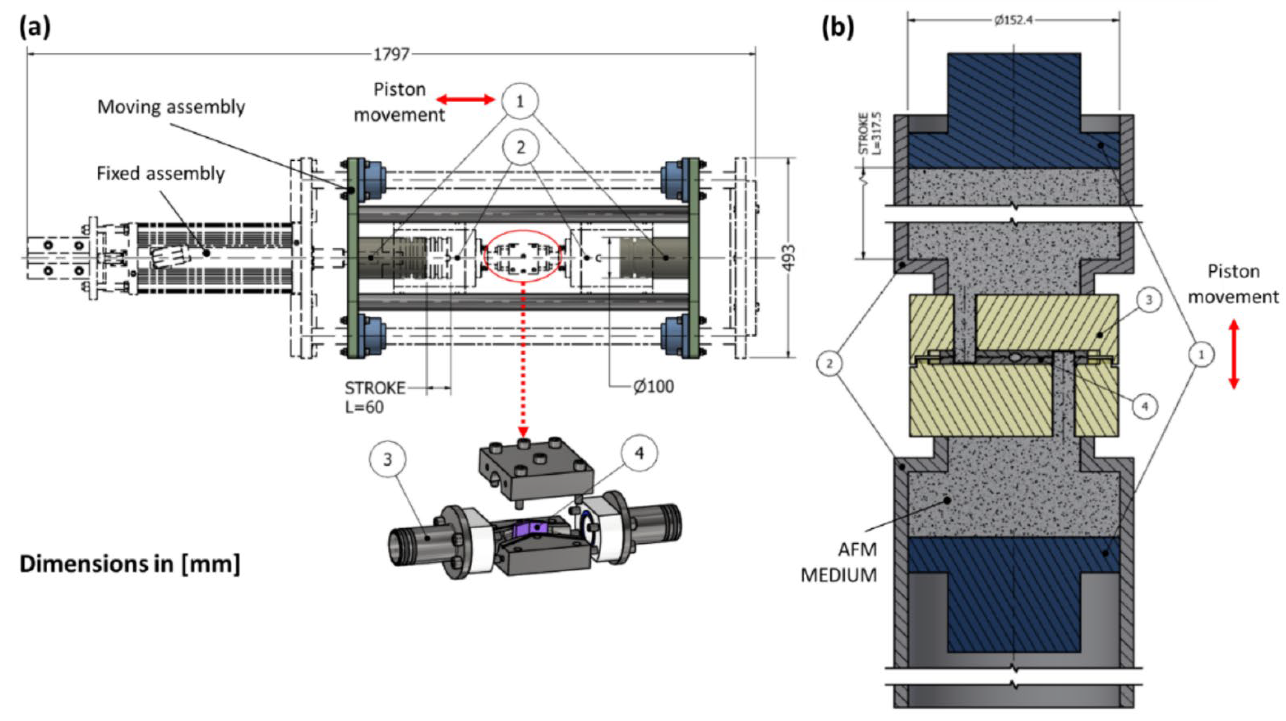
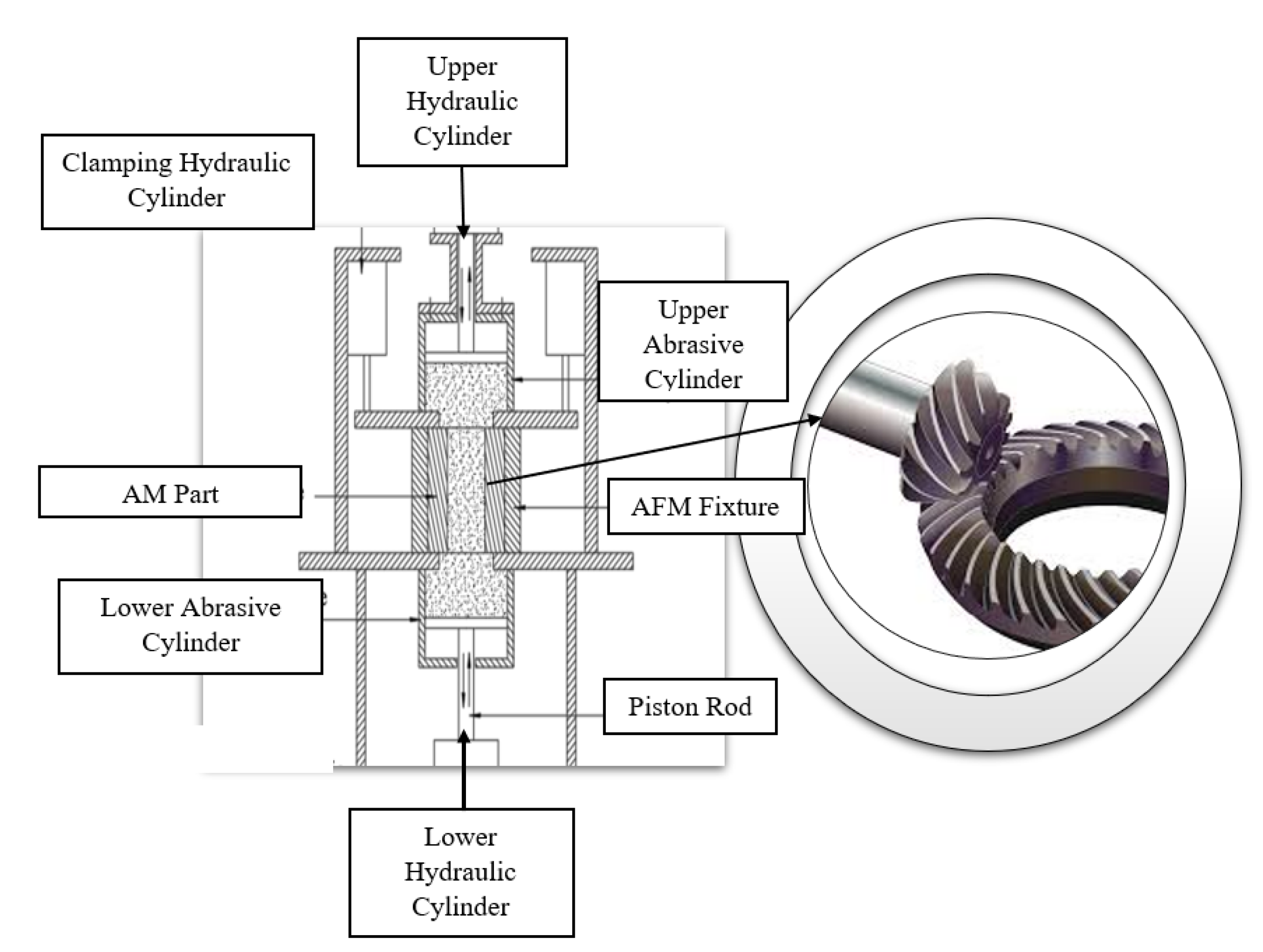
1.1.2. Abrasive Flow Machining (AFM)

AFM is considered to be the non-conventional process of finishing that deburrs, polishes, alleviates the recast layers, and has the potential to generate the “compressive residual stresses” at the part where it is difficult to reach with the conventional finishing process. Few of the major applications of AFM include the finishing of various aerospace and medical components, automotive parts, and high-volume generation of electronic parts. Several materials such as soft aluminum, ceramics, tough nickel, and carbides have been micro-machined successfully through this process [36]. The process of AFM gives the high-level surface finish as well as close geometric tolerance at reasonable and economical rates for a significant range of industrial parts and components [37]. One of the basic reasons behind implementing the AFM process is the ability of its media to finish the intricate points in the components where it is difficult to reach using conventional methods. Also, it can follow the “complex contours” and work simultaneously on several edges and surfaces, thus making it more desirable in comparison to the other finishing processes [38]. In the manufacturing process, several mechanical parts undergo one machining operation at least once in order to fulfill a certain function within the environment [39]. Some criteria for the quality of such pieces are desired, such as dimensional, roughness, as well as geometric specifications, etc.
AFM alleviates small quantities of the material through “semi-solid abrasive laden media” across the workpiece. In this process, two vertical cylinders opposing each other extrude the media in both directions (back and forth) across the passage in the workpiece as well as tooling, as shown in Figure 6. Here, the media comprises the abrasive grains and that of the semi-solid carrier, where the media acts as a “self-deformable stone” possessing protruding abrasive particles that act as the cutting tools.

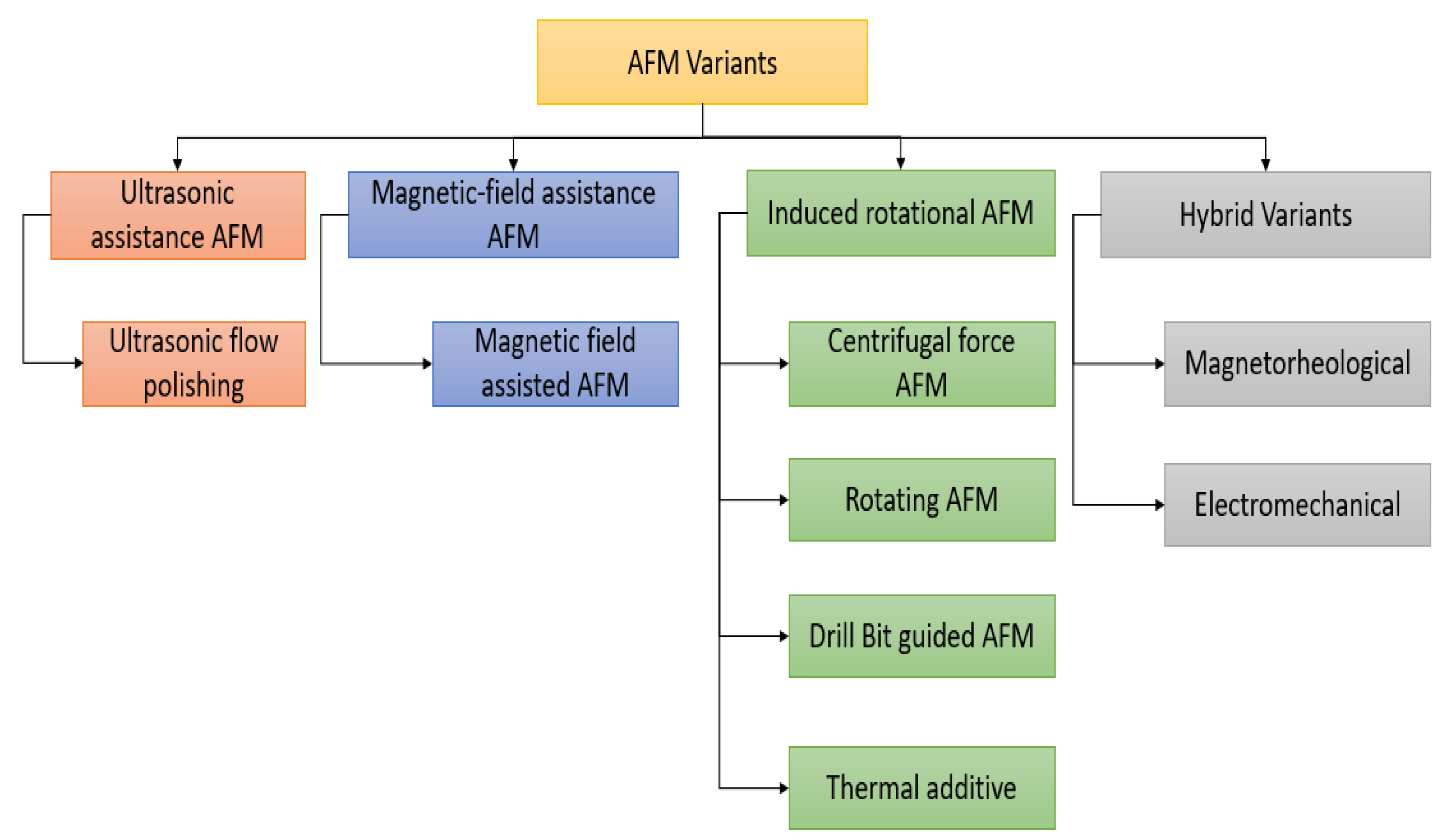
1.1.3. Developments in AFM Process

The abrasive flow machining process can provide good results for the machining components that need the removal of the defects created by the mechanical or manufacturing processes. The AFM process makes ideal for relief of surface stress, radiusing, polishing, deburring and geometric optimization [41]. Being an essential requirement of industry these days, a large amount of research work has been reported in this domain in literature.
AFM is considered to generate the “self-deforming tool” that accurately removes the extra workpiece material and then finishes the surface from the areas where it is difficult to do so with the conventional machining process [42].
The material removal process comprises three modes of deformation, which are as follows:
  • “Elastic deformation”: it correlates with rubbing
  • “Plastic deformation (ploughing)”: it correlates with the material being displaced without being alleviated.
  • “Micro-cutting” [43,44,45]
Initially, in [46], the authors developed the one-way process of AFM where the medium traveled in a single direction and termed it to be the simplest type of AFM that consumes the least time during the finishing process [47,48,49,50]. It was observed that surface roughness could be minimized to 90% on the machined, cast, or EDM surface having the “dimensional tolerance” up to or ±0.005 mm [51,52].
In order to get a better radiusing and finishing action not only in the inner but outer surface as well as the components, two way AFM process of finishing was developed [53,54]. Its basic operation involves two horizontal or vertical hydraulic cylinders that lie opposite each other and are placed in between the work piece with the help of suitable fixtures, as illustrated in Figure 7. The pistons in the cylinders are used to make the “abrasive laden medium” move back and forth on the surface that needs to be finished. In this way, the finishing process is carried out in a two-way AFM operation.
In [55], another development was made regarding the oscillatory motion of the workpiece. With oscillations to keep going, the work piece hits the “abrasive medium” with the “eccentric path” that causes the intricate and complex structure to make an interaction fully and completely with that of the abrasive medium, which results in the same (equal) abrasion on each side of the components. In [56], an AFM setup has been developed on the lathe to carry the experiment on brass as well as aluminum. It was observed that the dominant factors are the “abrasive concentration” in the medium, followed by the mesh size, speed of the medium flow, and the number of cycles. A lot of improvement could be seen in the case of materials that were soft, considering the surface roughness enhancement. In [57], the temperature has been considered to be the most influential parameter in the AFM process regarding work efficiency; with the escalation in no. of cycles, the medium temperature increases, which means the decrease in the medium viscosity occurs with the increase in no. of cycles. In work, it has been presented that in AFM testing, an increase in no. of cycles significantly decreases the material removal rate (MRR) as well as surface roughness, thus reducing the efficiency [58].
In order to enhance the process performance and control the rheological properties, scientists and researchers have designed and developed several AFM process variants [59,60] by combining and incorporating the basic AFM operation with that of the traditional/non-traditional flow machining operation. The process of AFM has been classified as per the energy and forces used within the process [61].
Other than the above-mentioned four types of AFM process, there have also been developed some other AFM variants in order to compensate for the MRR and also for a longer finishing time. The variants of the AFM process have few external assistants, such as ultrasonic vibrations [62,63,64], the rotational effect [65,66,67], magnetic field assistance [39,68,69], and also the hybrid variant of the AFM process [54,70,71,72]. The external assistance is found to show the increase in the finishing force [73,74,75], abrasive velocity, enhancement in the contact length among the work surface as well as abrasive, active density of abrasive, or utilization of the synergic effect of two processes in order to eradicate the material [76]. These effects result in enhancing the finishing time, MRR [62,63], and surface roughness. The further classification of the developed AFM variants has been shown in Figure 8 below.
A summary of the differences and similarities of the different AFM process variants is shown in Table 2.
In order to give the best control on the AFM processes, the selection of the parameters of the process is necessarily required. This review paper has segmented the AFM process parameters into three main categories. The classification of these three main AFM parameters, including machine, medium, and workpiece [77,78,79]. Here, the machine decides the level to which the abrasion can be processed through “viable extrusion pressure,” flow rate, flow volume, and also the number of cycles [80,81]. “Rheological properties” of “abrasive laden medium” are the ones that signify the amount of abrasion. The grit size, viscosity, temperature, and polymer to dilute are considered to be the parameters for comprehending the rheological properties of the MR fluid. Next comes the workpiece that is finished by the AFM process. The properties of the workpiece, such as material type, roughness value, and also geometry, tell the machining time and abrasive type to be used [82].
Summary of the performance analysis of the AFM process regarding their process parameters is shown in Table 3.
The typical defects during different manufacturing processes for electronic components, pipes, welding parts, and textile materials can be improved using the abrasive-based machining process, i.e., the AFM process and its variant processes, as shown in Figure 9.
Hashmi et al. also have discussed the various surface defects occurs during additive manufacturing processes i.e., staircasing/stair-stepping effects. Authors have discussed the various post-processing techniques including abrasive-based machining methods for removing the surface defects of these additively manufactured parts. Authors have also discussed the machine vision technique or artificial intelligence-based technique for measuring the parameters of machining processes [88,89,90,91,92,93]. Authors have also discussed the experimental investigation of the AFM process to improve the surface finish of polymer-based AM parts [94,95,96,97].
A summary of the process performance analysis of abrasive-based machining processes in different applications is shown in Table 4.
In the present research work, different research related to mathematical modeling and simulation methods for abrasive-based machining processes is categorized to provide a valuable study for the researchers in the exciting field of computational analysis. As a result, new ideas in the mathematical modeling and simulation methods and research gaps in the existing literature are obtained. Future research works are also suggested to push forward this interesting research field. Section 1 presents a review of research works related to the general overview of abrasive-based machining processes and their types. In Section 2, research works are classified according to the different topics in research to the mathematical modeling and simulation approaches for abrasive-based machining processes. In Section 3, research works are classified according to the various topics in research to the simulation techniques for abrasive-based machining processes. In Section 4, research works are classified according to the various topics in research to the mathematical modeling for abrasive-based machining processes. In Section 5, the conclusions of this literature review have been discussed, and future research works in the field of mathematical modeling and simulation of abrasive-based machining processes are also suggested. This review paper provides deep insight into the current developments in AFM processes, abrasive media, their modeling as well as optimization, and various promising application domains.
Since the paper mainly focuses on the modeling and simulation techniques of abrasive-based machining, the next sections describe various other modeling types and simulation processes of AFM.

2. Mathematical Modeling and Simulation Approaches for Abrasive Machining Processes

Recently, computer simulation applications have proved their efficiency in solving complex problems in Engineering. Different techniques of modeling and simulations are considered widely in the Industries, such as “computational fluid dynamics (CFD)” [83,104], “discrete element method (DEM),” “finite element method (FEM),” “artificial neural network (ANN)” [14], “multi-variable regression analysis (MVRA)”, “response surface analysis (RSA)” and “Stochastic modeling (SM)” [105]. These techniques have several applications in the industrial process, such as predicting the behavior of the material removal in loose abrasive-based machining [106]. The results obtained from the modeling and simulations pave how to optimize the process parameters that affect the finish of the workpiece. Several researchers have prominently worked on the “mathematical modeling and simulation” of “loose abrasive-based finishing processes.” Several experimental as well as computational techniques and approaches have been performed to analyze the ideal and optimal procedural parameters [103,107,108,109].

Classification of Modeling and Simulation Techniques for Abrasive-Based Machining Processes

The modeling and simulation-based techniques for LAM may be classified based on the used techniques, i.e., “computational techniques and statistical techniques Petare et al. have also classified several simulation techniques [110], which are shown in Figure 10.
Based on the classification presented in Figure 9 above, the detailed description of each classification has been elaborated in the next sections.
A summary of the shortcomings of simulation techniques for Abrasive-based machining processes is shown in Table 5.

3. Review of Simulation Techniques for Abrasive-Based Machining Processes

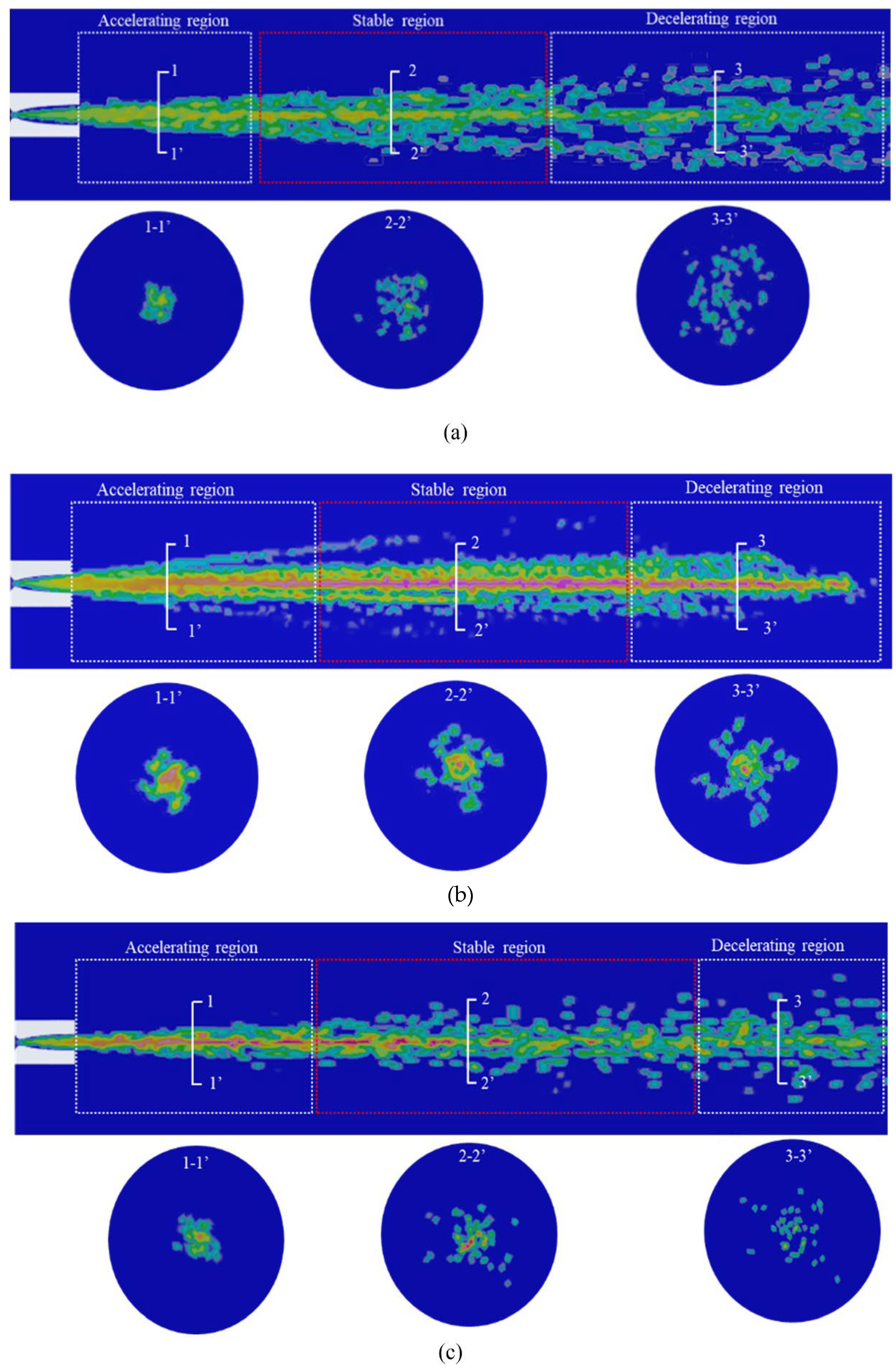
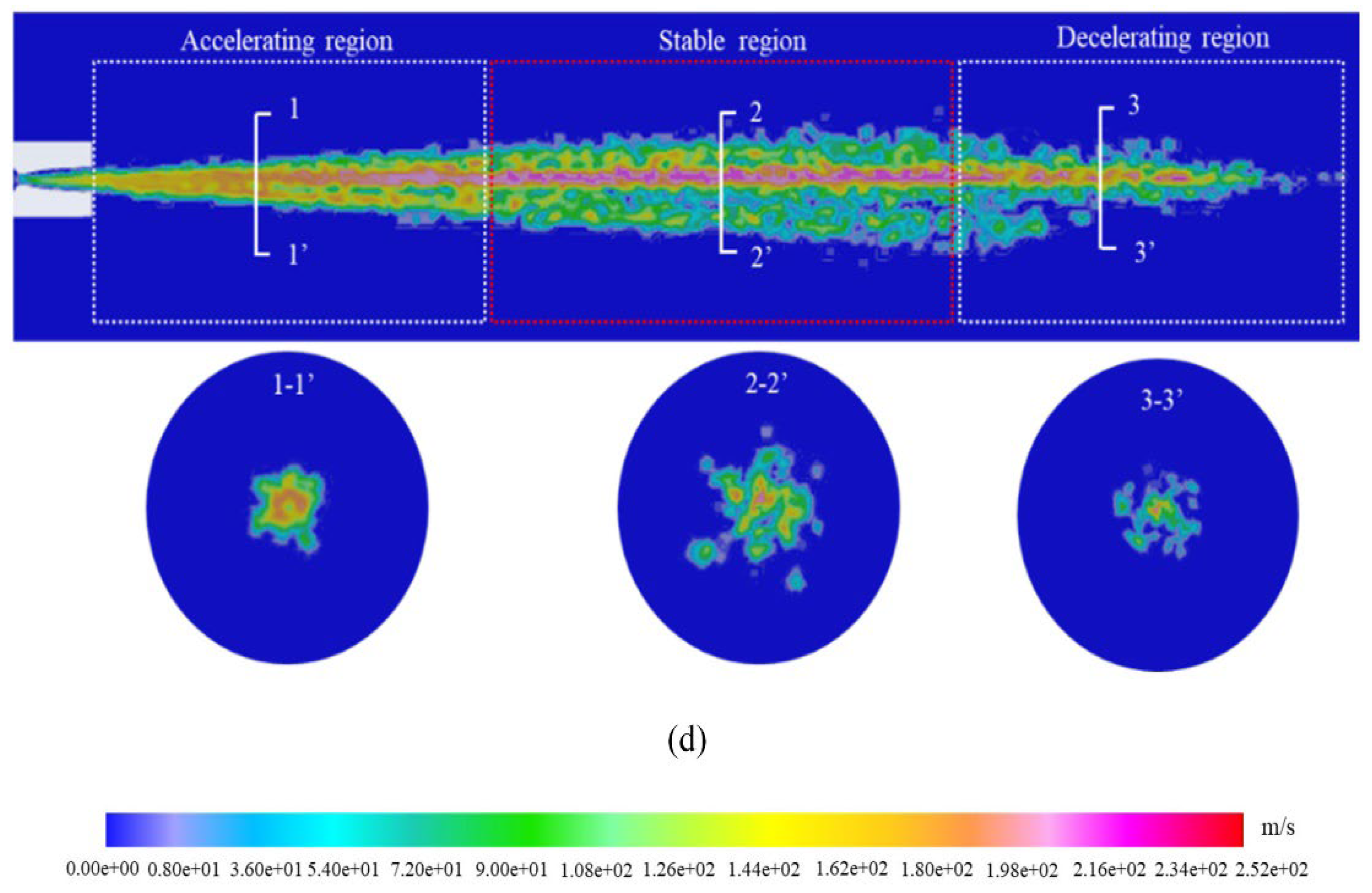
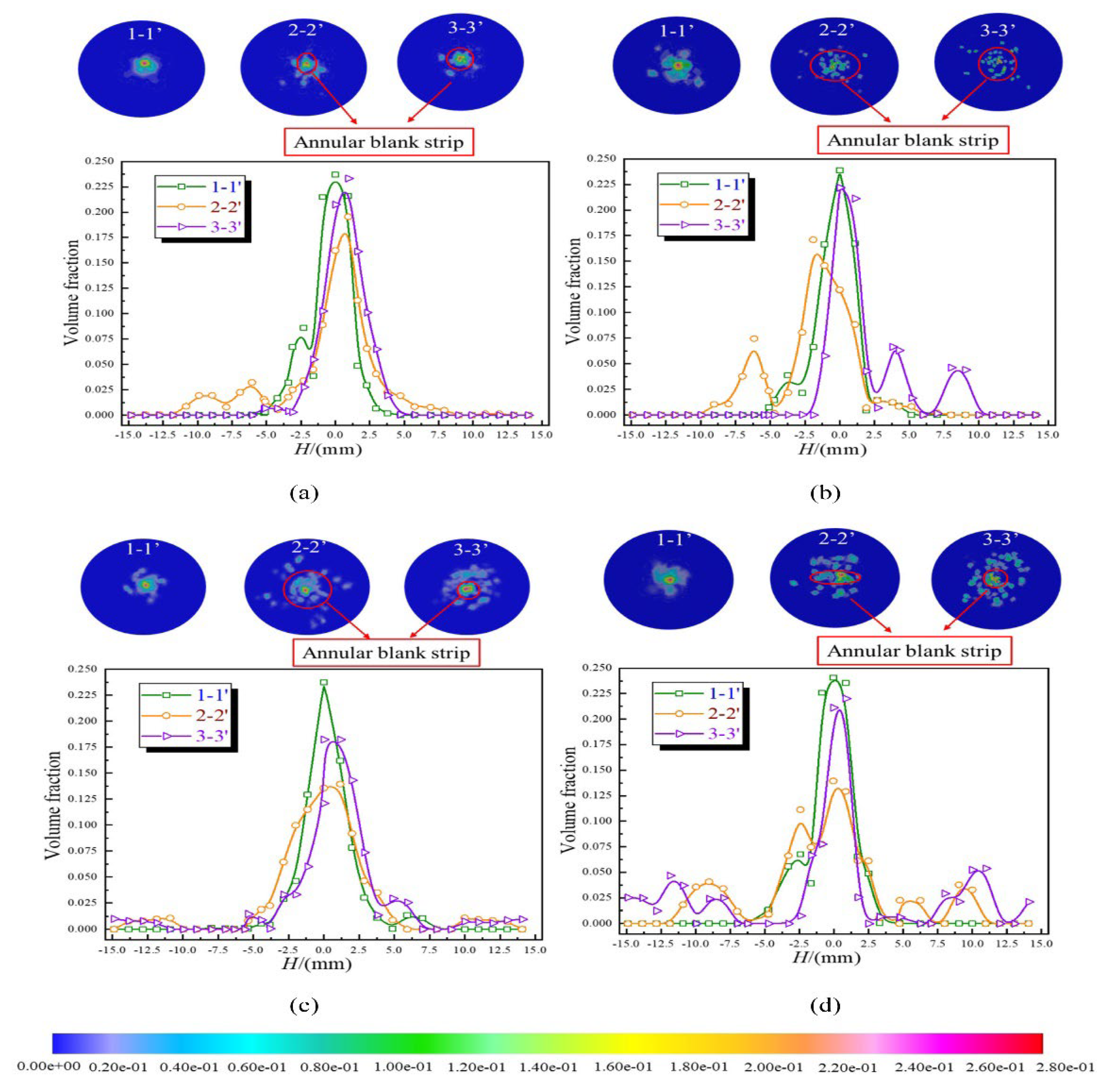
3.1. Computational Fluid Dynamics (CFD)

This approach is applied to simulate the fluid flow problems in any system aided by numerical methods by integrating the problem’s equations. The characteristics of shear-thinning, Newtonian, non-Newtonian, or the Maxwell fluid are considered while choosing the equations of Navier-stokes to model the flow problem. This method is also applied to take various flow channel geometry into account, locate the optimum parameters for the process, and reduce cost. The simulation performed by Computational fluid dynamics is performed using the available commercial software such as ANSYS ACE, ANSYS CFX, and ANSYS FLUENT using Ansys 2021 R1 software version developed by “Ansys”, was founded in 1970 in western Pennsylvania, United States of America. The general working steps that happen inside the software to apply the CFD approach are shown in Figure 11 below.

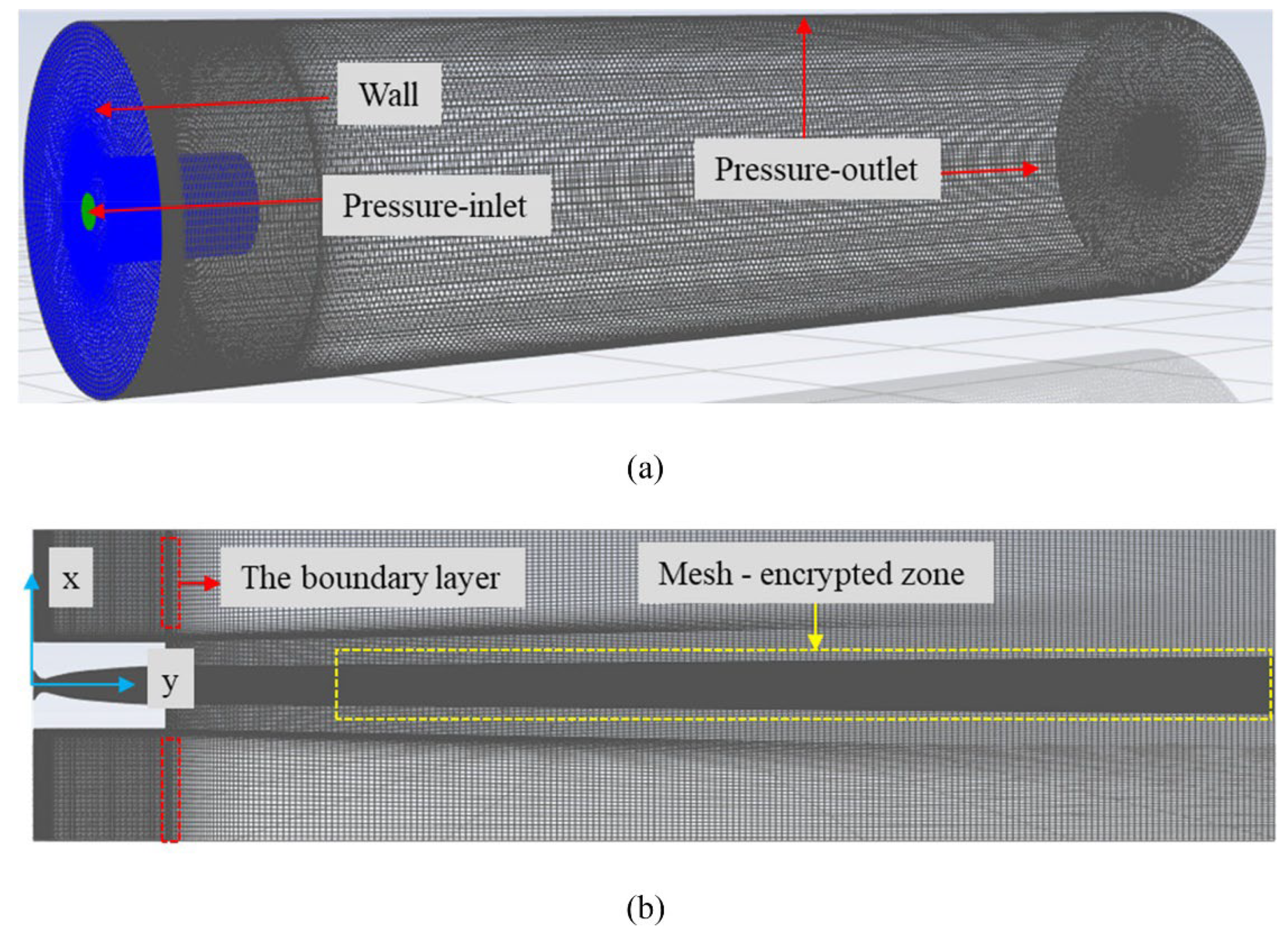
3.1.1. Pre-Processing

In this step, the model of CAD that defines the fluid domain in our problem, including any solid boundaries, is prepared first. This step is followed by giving the CFD solver’s required initial and boundary conditions to run the simulation. The other conditions, including the physics needed for the problem along with the meshing conditions, are also fed to the commercial code used for the CFD simulation of the problem. This initial step of creating the CAD model can be performed under the same roof within the software used for the flow simulation itself [111].

3.1.2. Meshing

Meshing is a process of discretization where the fluid volume is converted into many more minor elements or volumes. However, many discretization methods are available, and most CFD software uses the Finite Volume Method (FVM), while some exceptional CFD tool uses the Finite Element Method (FEM). The Meshing mechanism involves sub-dividing the extensive computational domain into many discrete cells called finite volumes (or finite elements if FEM occurs) depending on the CFD toolbox used. The mesh can range from structured or unstructured, uniform or non-uniform, and even with multiple elements like hexahedral or polyhedral in the mesh domain. Meshing remains the main paramount parameter for a CFD simulation to work as desired. Any irregularity in the mesh will crash the simulation when run by the solver [111].
Due to the complexity of Partial differential equations, it is difficult for them to be solved using the computer; therefore, they are converted to another form to be solved in the computer. This process is called discretization, which provides getting continuous equations. By solving a matrix, the algebraic equations can be obtained from the Partial differential equations, and to do that, it is required to identify points. The discretization method is also known to be the “Finite volume method.”

3.1.3. Solving

This step is where the actual application of the CFD technique happens. During this step, the CFD software solves the unknowns present in the Navier Stokes equations. The linear system of equations is solved iteratively, coming up with a better value after each iteration. When explicating the integration scheme, the uncoupled equations can result from the linear system, whereas the coupled equations can result from the implicit equation. With turbulent flow problems, k-epsilon and k-w equations are solved used, and with a laminar flow, the normal Navier-stokes equation is solved.

3.1.4. Post-Processing

The results are obtained in this final step, where the pictorial depiction of the flow parameters is exported and used to study the problem further. Many plots from various sections depicting the distribution or the flow parameters are conducted in post-processing using inbuilt tools or open-source tools like ParaView.
With the advancements coming up in the industrial process, there is an essential role for the process safety in operation and the design of the process facilities. A significant effort was paid to ensuring that “chemical process industries” are at the safest and most secure workplaces among several other industries. However, there is a requirement to analyze the safety of the process mechanism to predict the scenarios. Using experiments to quantify the process safety mechanism is considered to be insufficient as it is highly “resource-intensive.” Fortunately, with the increase in the capabilities of the computation and the enhancement in the “Computational Fluid Dynamics (CFD)” tools, the study of hazardous scenarios and the fundamental mechanics have been improved [112] and has become sophisticated [113]. This approach can model the fluid by solving numerical equations besides capturing the effect of viscosity. CFD can also predict chemical reactions, mass and heat transfer, and fluid flow [114,115]. CFD also has several applications in modeling and simulation in the engineering field [116].

3.1.5. Applications

The thermodynamic and hydrodynamic performance of crude oil before heating in refineries is impaired by fouling. There are inappreciable fouling levels at the early stage of fouling which cannot be determined due to the lack of data from the experiments. Therefore, computational fluid dynamics (CFD) is applied for a better understanding. The CFD technology can account for the chemical reaction, the turbulent flow, and the aging in the tubes present in the heat exchanger. The study [117] simulated three-dimensional CFD under different operating conditions to predict the deposition rates and determine the importance of the fouling mechanism. The interaction between the processes of precipitation fouling and the chemical processes can be characterized by the “interference factor” used to evaluate the suppression extent of the chemical mechanism [117].
The firing range depends critically on the ventilation systems for exposure to ammunition refuse personnel. CFD is used to simulate the ventilation system and predict airflow patterns. The purpose of this model is to identify back circulation, which emits fire. The validation of the solution of the model and the input parameters of the model are the values measured at several locations. It has been evaluated using the analysis of the massless particles fired at various heights corresponding to kneeling, standing, and prone firing positions. Using the recommended technical guidance for the ventilation of the firing ranges of the small arms compared to the dynamic flow of the system, different predictions are finished. The results showed that the particles return behind the shooter [118]. The air velocities of lower supply correspond to the particle’s successful movement and the uniform flow under investigation in a small firing range. It has been demonstrated that the models of CFD are advantageous as it provides optimization in the air velocity of the supply and enhances the design standards [119]. CFD is also used to model the 3D Concrete Printing to predict the shape of cross-sectional 3D printed segments, which can be achieved through the simulations of “virtual printing.” It has been found that the numerical results of CFD are appropriate to the results of the performed experiments [120].
CFD has the edge over the other modeling methods because of the sophistication available at its disposal. The angle of the impact made by the abrasive particles upon hitting the target surface in Ultrasonic Assisted Abrasive Flow Machining (UAAFM) could be visualized from the simulation results, and its outcome is therefore evaluated. With the results obtained from the CFD model of the UAAFM, the effect of the temperature rise on the media stability can be predicted, and major decisions could be undertaken [121]. The abrasive wear on a turbine blade’s surface can also be evaluated, helped by CFD simulation. The study helps to identify the effects of the size and shapes of the quartz particles on the abrasive and corrosive attrition of the blade [122]. Kim et al. have investigated the deburring of AL6061 material using the AFM process. The authors have conducted the experimental study and three-dimensional CFD simulation of the deburring process and compared both experimental as well as numerical results [123]. Fu et al. have also investigated the rheological and finishing behavior of AFM media using the experimental study as well as CFD simulation study [124]. Pradhan has compared the experimental and CFD simulation results to predict erosion behavior during hot abrasive jet machining (HAJMing) [125]. Similarly, authors have modeled the HAJMing process using CFD analysis [126]. Amar et al. developed the analytical and numerical models for abrasive water slurry jet machining (AWSJM) to fabricate the micro-channel using experimental study and CFD simulation, respectively [127]. Zou et al. simulated the precision machining of straight internal gear using the large eddy simulation method on the CFD platform [128]. Chen et al. [129] have characterized the motion of abrasive particles using CFD-DEM modeling for the abrasive air jet machining process. The authors have analyzed the effect of nozzle pressure ratio (NPR) on the flow field of abrasive particles and stress distribution on the workpiece for the optimum parameters of abrasive air jet machining. The mesh model of the physical model used for CFD-DEM modeling and a few important simulation study results are shown in Figure 12, Figure 13 and Figure 14.
Zhang et al. have simulated the behavior of visco-elastic AFM media on micro-slit structures using the CFD simulation technique. The authors have concluded that the flow time (21 s), which was calculated at a velocity of 1.2 mm/s, further demonstrated the polymer chains’ remaining stretched state [130]. Similarly, the authors have also simulated the flow of abrasive media using the CFD simulation technique by adopting the carreau-yasuda and wall slipping models. The rheological behavior of AFM media is affected using a material removal mechanism [131]. The mesh model and a few results of these CFD simulations are shown in Figure 15 and Figure 16 below.
Zhang et al. [132] numerical investigated the machining (AFM) of micro-porous structures using the CFD simulation technique by Brid-Carreau model coupled with mixture and discrete phase models. The authors have demonstrated the simulation results and surface morphology for the finishing of the micro-hole, as shown in Figure 17, Figure 18 and Figure 19.
Zhu et al. [133]. used the double cosine kernel function (SCKF) to develop semi-resolved CFD-DEM for investigating abrasive air jet (AAJ) and studied the particle-scale distribution information in the nozzle of the AAJ machine. Some important results of this simulation study are shown in Figure 20 and Figure 21 below.
The summary of CFD-based modeling and simulation of the loose abrasive-based method is shown in Table 6.
Even though the CFD simulation model has the edge over other processing models, a lot of advancement has occurred in other simulation models. The finite element method-based simulation model is one of them. The next section describes the significance of FEM simulation-based processes.

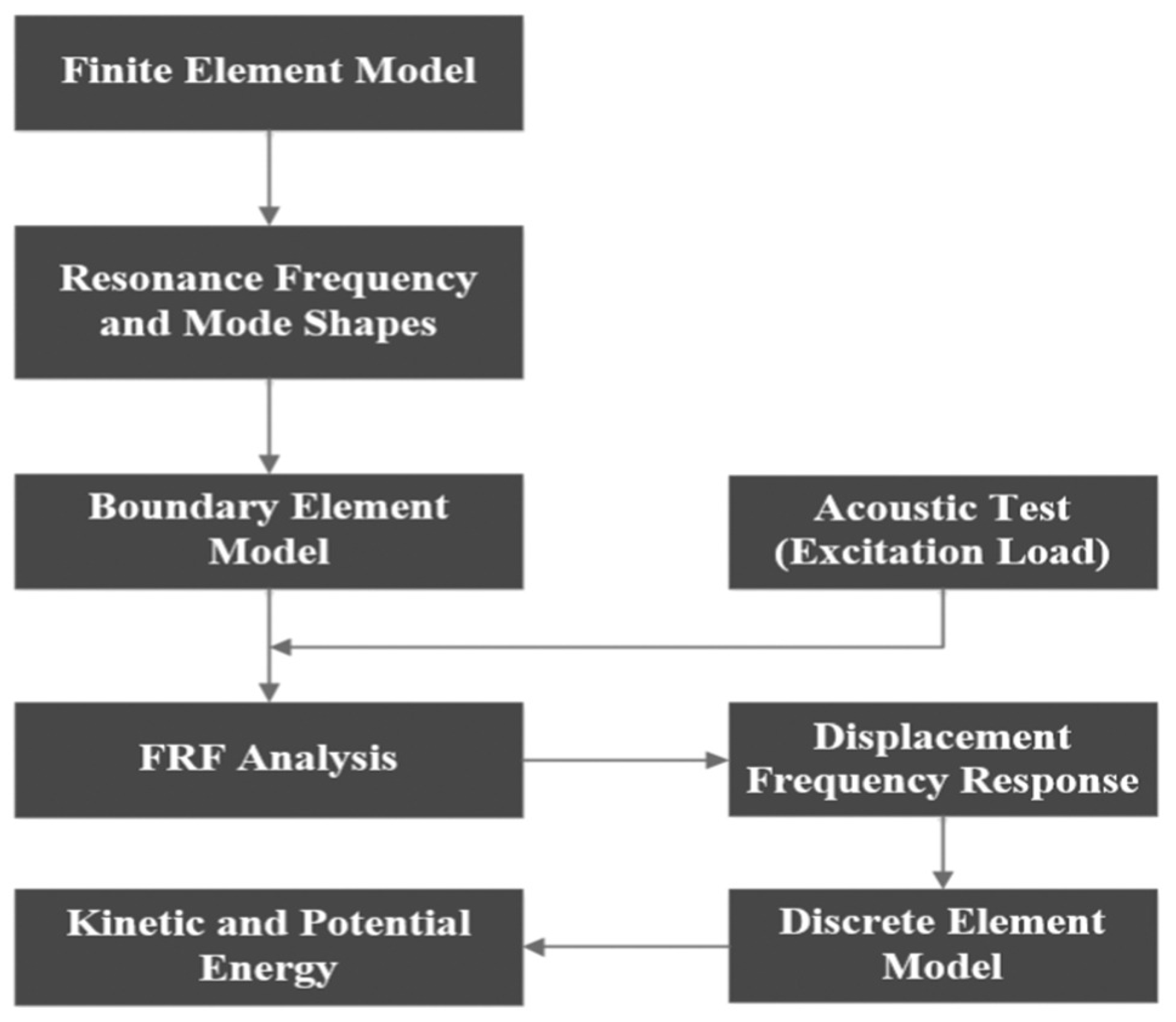
3.2. Finite Element Method (FEM)

The techniques from the Finite Element Method are adopted to predict the surface roughness in a more efficient method of magnetic abrasive finishing (MAF), named “ultrasonic-assisted magnetic abrasive finishing (UAMAF)” [135]. The effect of strain hardening is not considered in different modeling techniques [136]. However, there is a significant role in this effect to play. Also, the effect of heat transfer is neglected in other techniques, and only the mechanical problem is considered. The finite element technique can overcome this problem besides solving the nonlinear problems. Also, it is possible to analyze thermomechanical through the advancement in the software. This approach utilizes the techniques of “numerical practices in metal machining”. Replacing the range by “finite elements” forming a mesh is considered to be the basic principle of this approach called discretization. The accuracy of the simulation of FEM does not depend on the digit numbers; however, with the increase in the number of the equation, the accuracy is also increased. For the FEM modeling, the available commercial softwares are more trusted than the manual programs. The steps of applying the FEM approach are represented in Figure 22.
The Finite Element Method (FEM) was developed in the 1960s by Clough in his book “The finite element method in plane stress analysis”. This approach is used in spatial modeling and has several applications, such as modeling aircraft structures [137,138]. This method can be defined as a computational technique used to obtain approximate solutions in engineering for boundary value problems. This approach allows permitting the continuum to be discretized into finite elements. By assembling the discretized elements as per node properties, it is easy to estimate the continuous domain. Therefore, the FEM has been applied to solve several problems in engineering and applied science [139,140,141].
Several researchers have used FEM analysis for the simulation of the process of solid particle erosion that occurs in abrasive machining [142,143,144,145,146]. In [147], the author has simulated the impact of several spherical particles using the 3D FEM model and estimated erosion rates by calculating the average possible damage as well as extrapolating to level 1.0. However, the obtained results were in good agreement with the experimental results that have already been published in the literature.
In [148], the author used the FEM to simulate the “particle erosion process” by making use of the model of “elastoplastic material” with “failure criteria.” The changes in erosion rate with that of the particle velocity and impact angle coincided with the outcome obtained from the analytical and experimental procedures. Residual stress has also been analyzed, which is generated during the period of the occurring erosion process, and it was observed that the profile was similar to the one seen in the “shot peening process.”
In [149], the author has analyzed the influence of the “abrasive water jet (AWJ)” parameters on “geometric characteristics” of the erosion caters by making use of the explicit FEM and also verified the results by performing the experiments.

Applications

Boundary layer flow is one of the most important mechanics of the applications of fluid and nanofluid. These applications recently are limited to one-term approximations of similarity. The non-similar fluid boundary layer problems are used widely in the industrial field. The finite element method promises to solve ordinary differential equations with a boundary layer that is not similar. The study aims to complement and enhance the numerical heat transfer by using the technique of FEM as it can solve more than one system of boundary layer-derived equations. This approach’s obtained result is a robust technique when solving the boundary layer equations [150].
This approach has been commonly used in the test of beam bending to analyze the behavior of the cracking of asphalt mixtures. The internal structure of the Asphalt mixture has a great effect on the propagation of the crack. Besides the computational resources’ limitation, the asphalt mixture’s complex mesostructure leads to using the 2D simulation of fem in contrast to the 3D simulation. However, 2D modeling reflects the characteristics only of the microstructure of the section of one specimen, which precludes comparing the laboratory test results with the simulation results. To obtain several numbers of images of internal mesostructured, the technology of x-ray CT scanning was used. To construct the 2D fem model, image-based modeling has been used to simulate the tests of beam bending. It has been found that FEM modeling and simulations can predict the crack position [151,152,153].
Recently, adhesive joints have been used more extensively than mechanical joints because of the uniform distributions of stresses and lighter weight compared to mechanical joints. It has been found that adhesive joints are more appropriate with composite materials. To study the mechanical behavior of these joints, several simulations were performed. In these joints between the substrate in geometry and the adhesive, there is a scale difference. Therefore, the analysis using mesh generation is very difficult, and there is a need for the techniques of the manual mesh, which is sometimes not efficient, and the quality of the elements becomes worse. To overcome this problem, fem modeling and simulation are used. This method allows us to produce fine mesh by overlaying the local mesh patch on the existing mesh. Therefore, there is no need for re-meshing [154,155].
The Finite Element Analysis is conducted on the magnetic field to estimate the magnetic force needed for the hollow on the workpiece. The volume of material being removed by a particular indented abrasive is calculated to gauge the Surface Roughness. The study focuses on the relation between the Material Removal Rate (MRR) and the other parameters like the finishing speed, the nature of abrasive material, its size, and the concentration [156]. The finite Element Method is also the answer when it comes to modeling complex magnetic abrasive machining processes. It is being deployed to analyze the Cylindrical Electro-Chemical Magnetic Abrasive Machining (C-EMAM) performed on stainless steel (AISI-420) that is magnetic. C-EMAM helps achieve higher efficiency finishing when working on advanced material cylindrical jobs by abrasion and electrochemical dissolution. FEM aids in the calculation of the magnetic field distribution where the cylindrical workpiece is kept. The simulation results help in comparison with the experimental results of the material removed and the surface roughness and its validation [157].
The Finite Element Analysis also finds its use in the free abrasive polishing in an anhydrous environment to achieve stability during the polishing process. In the FEM Analysis, helped by an Infra-red camera, the effect of the pressure applied and the speed of rotation on the material removal is studied, along with the surface roughness. Other parameters such as heat generated are also evaluated and studied in this article [158]. Since its inception, the aerospace industry has seen many technological advancements, and current research focuses on advanced material alloys and composites. Due to the stringent requirements for the components to be used in the aerospace industry, exceptional accuracy, fatigue strength, and surface integrity are needed. Aerospace materials like Stainless Steel AISI 4130, Ultra high strength steel AF1410, and the AerMet 100 are employed due to their high fracture toughness and corrosion stress resistance. To retain the surface integrity of these substances, abrasive machining is used. The Finite Element simulations of these machining processes are used to predict and compare the results with their existing data from grinding models available [159]. The flow chart of FEM analysis is shown in Figure 23 below.
Zhang et al. have modeled the process of material removal on thermal barrier coatings (TBCs) using the abrasive water jet (AWJ) by new smoothed particle hydrodynamics (SPH)-based model. The results showed that There is good agreement between the analytical model and the erosion rate as the incidence angle increases [160]. Ozcan et al. have Modeled and simulated the controlled depth of abrasive water jet machining (AWJM) of free-form surfaces using the FEM method by signed distance field (SDF) approach. The authors have validated the simulated results from literature and experimental results [161]. Liu et al. have simulated the impact of high-speed abrasive particles on the tensile block of Al6061-T6 and Ti-6Al-4V materials using a hybrid approach of SPH-FEM. The authors have simulated the results of the material properties changes from the single impact of abrasive particles during erosion [162]. Similarly, Du et al. also have a hybrid simulation technique, i.e., the SPH-DEM-FEM method, to simulate the abrasive particle movement and wear of the nozzle during the AWJ machining process. The results showed that the mixing chamber and focusing tube intersection experienced the most significant wear. [163]. Vasudevan et al. [164] have simulated the AWJ drilling process using a hybrid method of FEA and SPH models. The authors’ proposed methodology to simulate the process is shown in Figure 24 and Figure 25 below:
Beigmoradi et al. [165] have investigated the polishing of 2024 aluminum alloy using acoustics energy by a hybrid approach of the FEM-BEM-DEM process. The proposed methodology for acoustic abrasive polishing using the hybrid FEM-BEM-DEM method is shown in Figure 26 and Figure 27 below.
Figure 28 shows the computational and experimental results’ primary phases of particle motion.
The summary of FEM-based modeling and simulation of the loose abrasive-based method is shown in Table 7.
FEM is considered to be the numerical method for the continuum materials; however, in DEM, there is no need for such an assumption. Furthermore, the FEM is considered to be the element-based method, while the other one is considered to be the particle-based approach. In this way, DEM is considered the most accurate method that provides results efficiently compared to the FEM because of the compatibility equation, linear response in FEM, and the constitutive relation. The detailed literature analysis of AFM methods using DEM has been discussed in the section below.

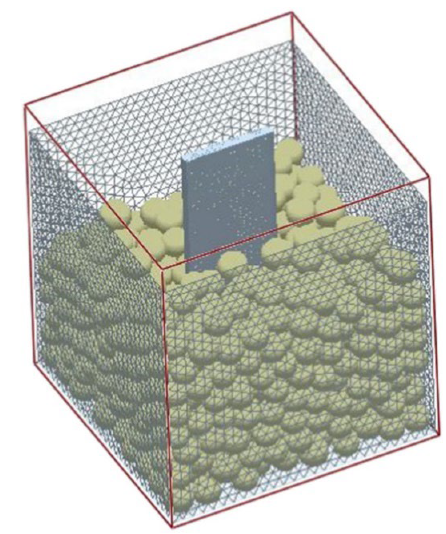
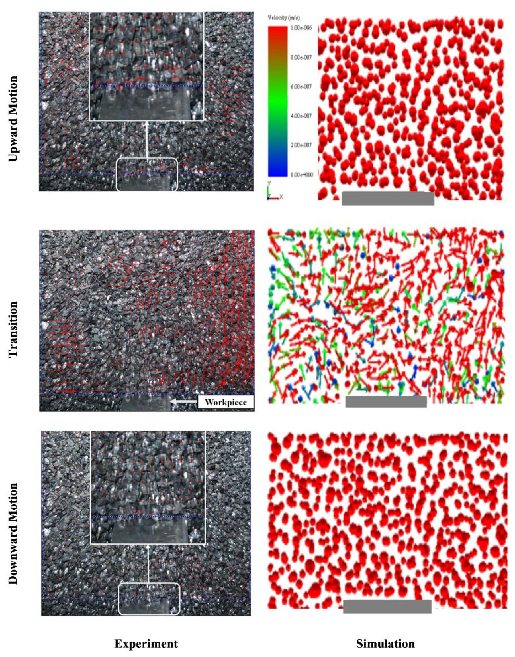
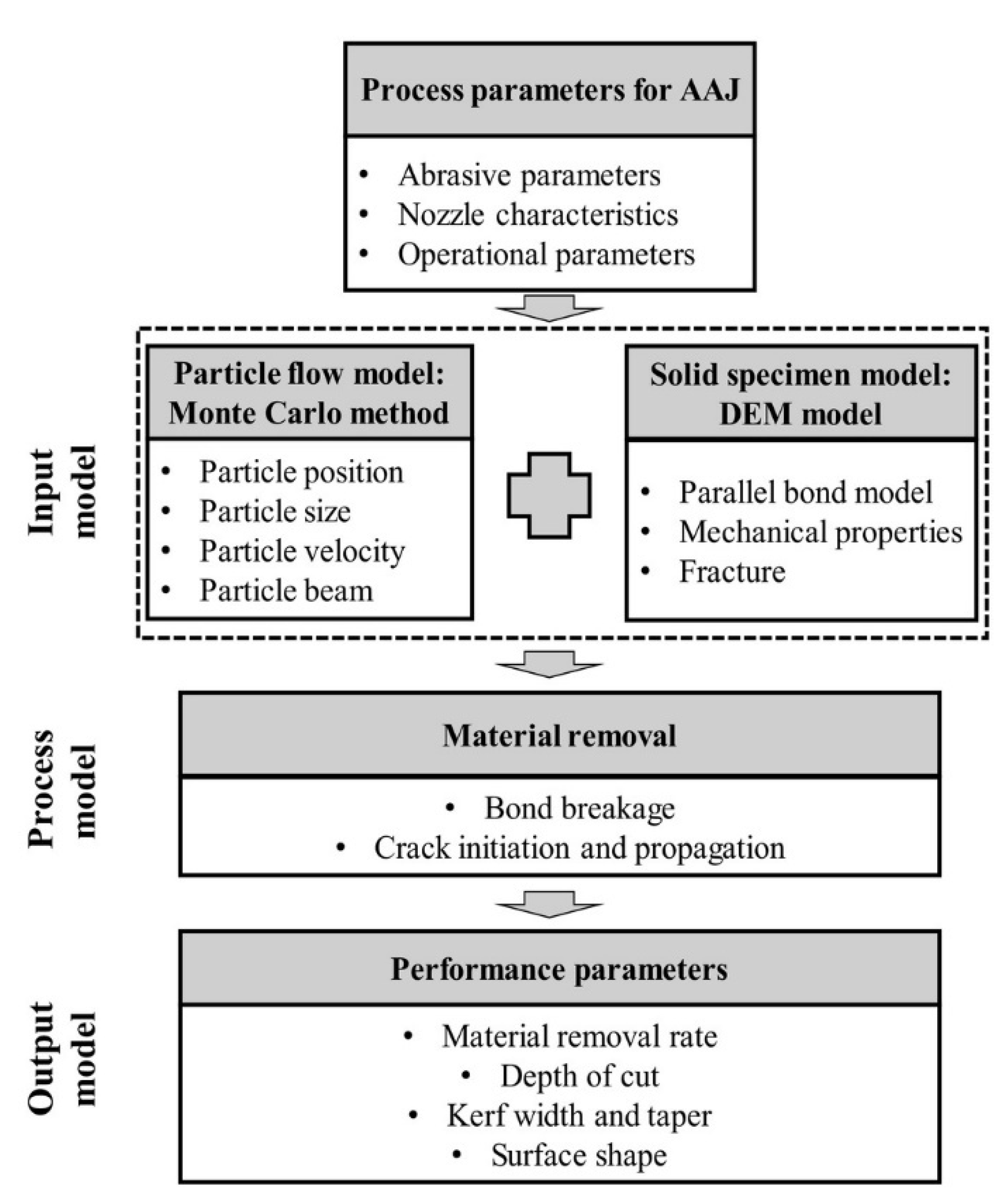
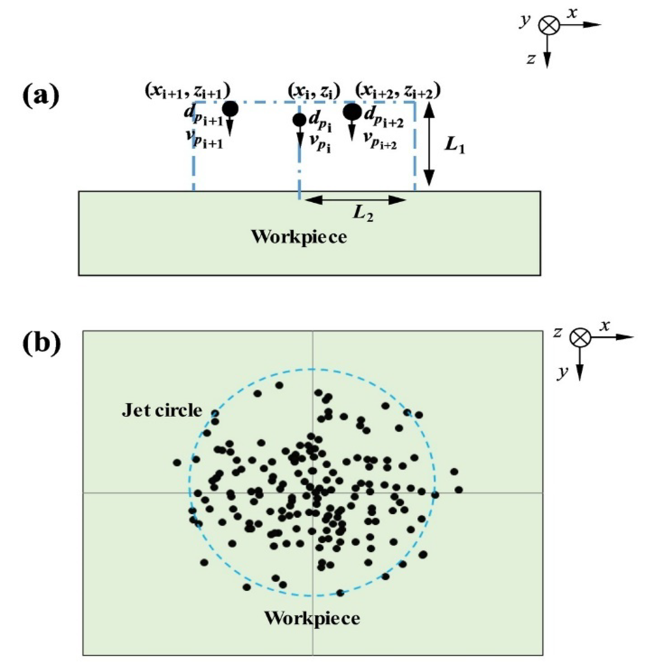
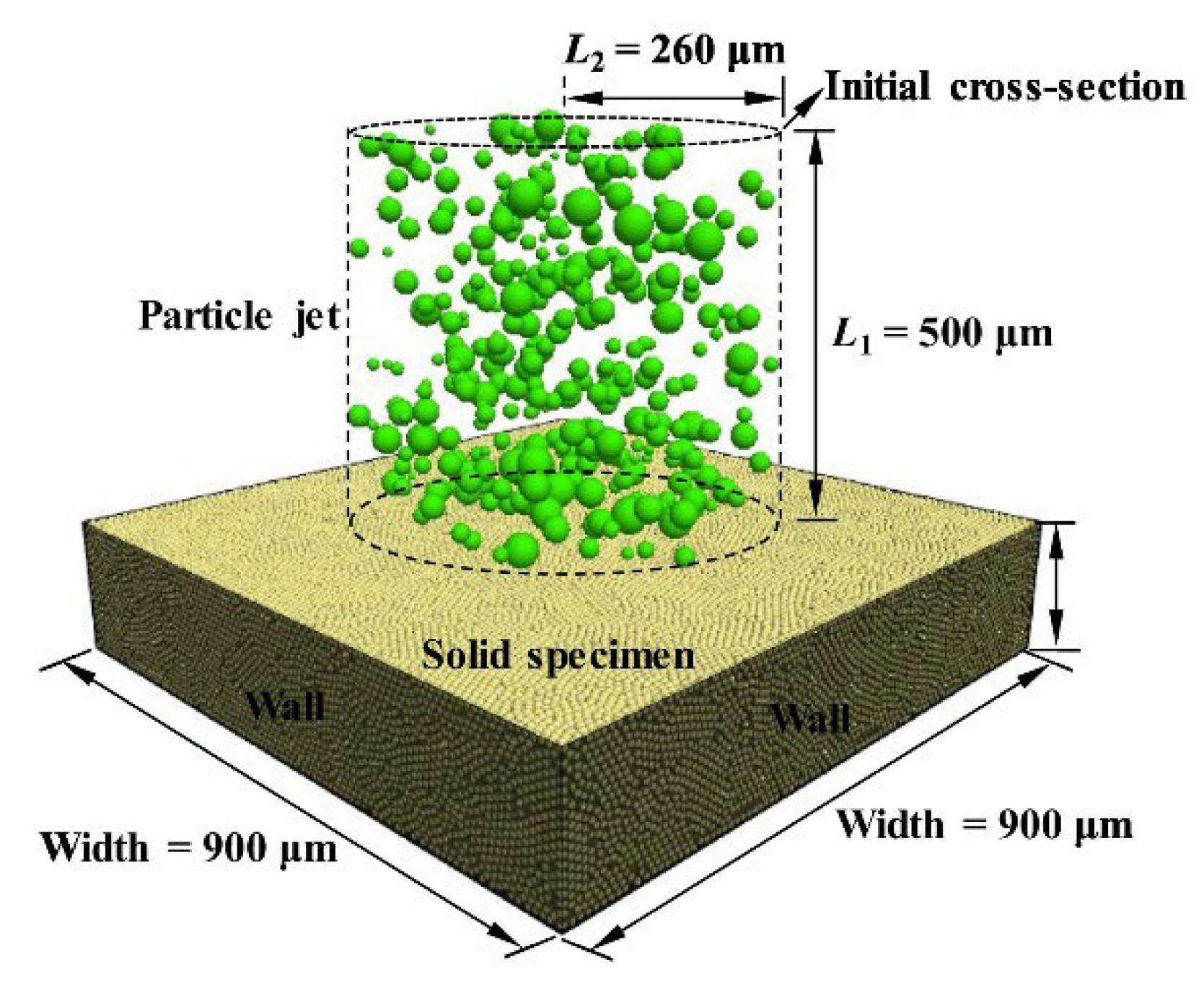
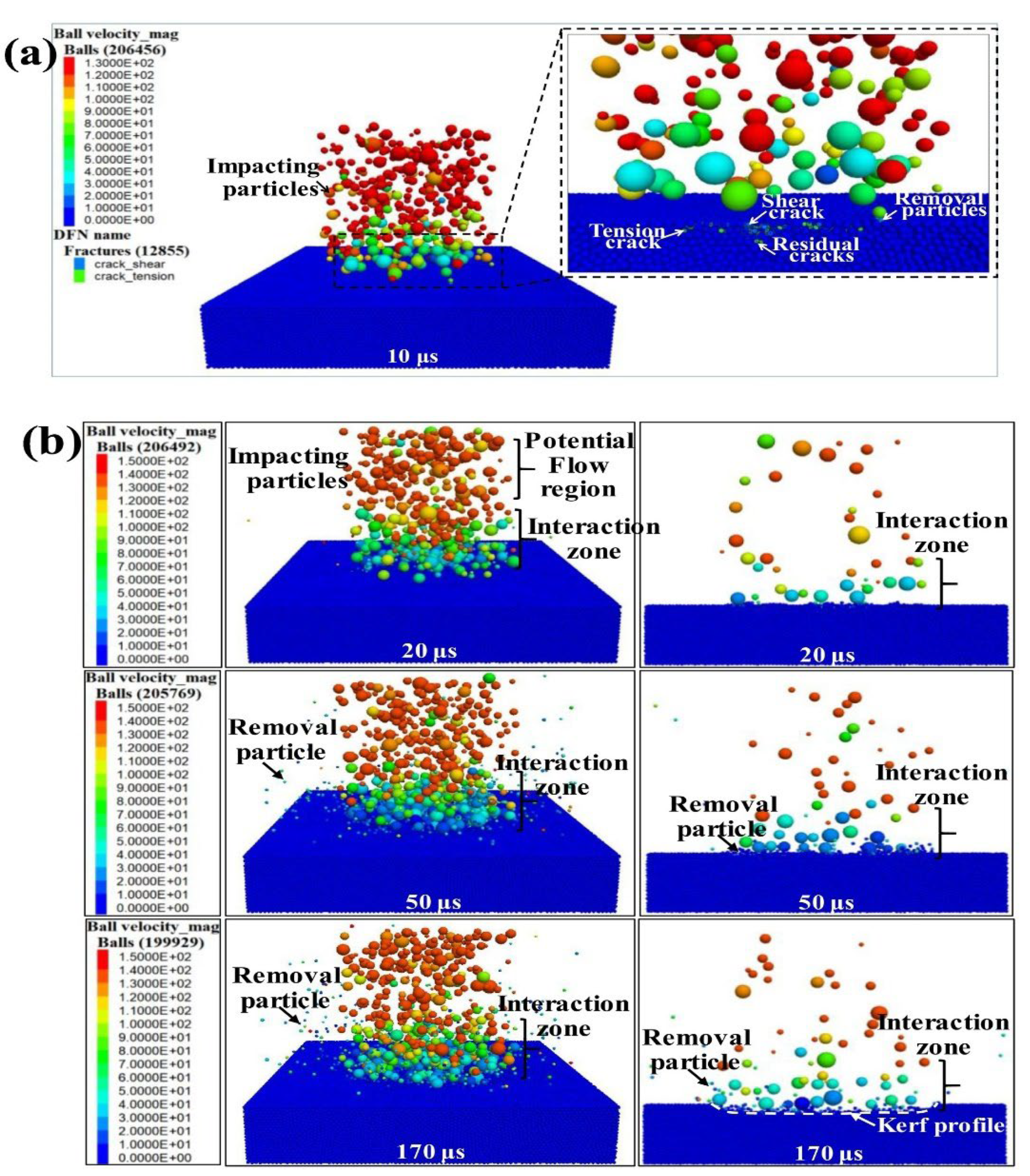
3.3. Discrete Element Method (DEM)

This method can be defined as a numerical particle size method applied to model the granular material bulk behavior. In this method, a numerical representation for each particle can be identified through specific properties. There are many physical phenomena in abrasive flow machining. By using numerical simulation, a piece of valuable information can be obtained to understand these phenomena. This method was developed in 1977 by Cundell to solve the problems of rock mechanisms.
There are three stages of the DEM mechanism [169].
  • Pre-treatment: to identify the arrangement of particles, geometry, and field and specify the physical field characteristics.
  • Dynamic calculation: the calculation of position, velocity, acceleration, and forces of the particles.
  • Post-treatment: numerical images and cutting force of the unidirectional composites machining during orthogonal cutting. Figure 29 shows the steps involved in DEM.
For modeling the microscale of the granular material, DEM can be used. The practical is evaluated as a separate entity through this approach, and the Newtonian motion equations are solved for each practical. The major challenge facing their usage of them is dealing with several objects. However, due to using the graphics processing unit (GPU) and to perform modern computer systems, this approach is used to solve many problems. Various types of spatial-temporal data can be resulted by using the simulation of DEM. This data has information about the particle velocities and positions. The calculation of DEM is performed in two-stage. These stages are the process simulation and the analysis of the data [170,171,172].
For the industrialized gross national product, the cost of abrasive wear is about 1–4%. Therefore, several studies were investigated to classify the various wear. These types are fretting wear, impact wear, fluid erosion, sliding wear, and fretting wear. To estimate the wear in various industries, especially in mining machinery, different types of numerical models were developed, consisting of two parts, an assessment of the wear and a simulation of the particle motion. The discrete element method has proved its efficiency in protecting the wear in different industries [173]. The Discrete Element Model allows directly modeling micro-mechanical parameters, such as the block’s behavior and the building geometry. This method also allows simulation of progressive masonry failure, the masonry structure dynamic behavior, and softening. The DEM simulations are performed using 3DEC software [174].
In [175], the authors have worked on the development of DEM simulations as well as coupled SPH for the scrutiny of the abrasive processes regarding the technical fluids in industrial applications. Here, these hold-ups are intermingled with that of the small solid particles that are held responsible for abrasive wear. Furthermore, in various other industrial applications, the suspensions represent viscoelastic behavior. In the presented research, numerical evaluation of the fluids based on the Oldroyd-B fluid has also been executed using the “SimPARTIXR SPH code”. Nevertheless, from the simulations of the “oscillator rheometer,” it has been observed that such simulation models are only for the crude approximation to the analysis of the intricate polymer fluids. In addition to these, a technique has also been presented enabling to numerically build the whole 3-D geometry of the single (abrasive) grains by making use of the DEM. The DEM-based abrasive grains have been used in coupled SPH simulation processes of AFM. Furthermore, the rheological simulations being performed for the suspension comprising the Newtonian fluid have also presented that executed simulations are in accordance with the experimentally collected data. This has made use of the suspension for the simulation of AFM.
In [176], inherent laws of the friction mechanism have been analyzed while the process of abrading is going on. The research presents that in the flow code modeling, abrading procedure is easy to simplify to the movement of such grains and particles in a “parallel-plate shear friction system.” For the said research, PFC2D software has been used to build the “particle flow friction system” along with the set of “parallel plate” as well as model parameters as per the equipment of the abrading procedure as well as the processing materials, and also through control simulation of single variation. Furthermore, a comparison has been made of the output data in order to approximate the impact of variation in parameters on the force chain. From the simulations, it has been analyzed that shear dilatancy is possible to be segmented into three stages: “plastic strain,” “macroscopic failure,” and “granular recombination.” Here, the load rates and the distribution of weak force chains rely on velocity, load, friction coefficient among the granular diameter, granules, and the number of layers of the granular. It has been observed that the load and granular layers upsurge the cause of the “direction of force chain” to be oriented with that of the vertical direction, and thus makes the force chain move in the horizontal direction with the increase in the velocity. With an increase in load, there occurs no variation in shear dilatancy stage, friction coefficient, and velocity. The flow chart of the DEM simulation-based model is presented in Figure 30 below.

Applications

The propagation modeling of cross-contamination of bacteria within bulk material is very important to validate the safety of the microbial of the tree nuts complex post-harvest processing. It has been found that the discrete element method is very efficient in modeling and simulating the propagation of complex bacteria during the material processing of bulk food [177]. Recently, the DEM approach became a promising alternative to the measurements of the physical properties of the systems of the thermal particulate. DEM has been widely used in several industrial applications. However, the simulation of DEM has not been used in a theory review that underpins the thermal simulation of DEM. Therefore, the study presents a comprehensive review of all thermal model majors and the heat transfer mechanisms using the DEM simulations [178].
Permeability of the bed is considered an important parameter in green iron ore pellet’s induration in the grate furnaces. For achieving higher quality, lower fuel consumption, and higher productivity, optimization and control must be pursued. The discrete element method is used to improve the permeability of the bed to control the green pellets distribution size to feed the furnace of the induration [56]. Handling the wet particles is very difficult in chemical engineering because of the cohesive acting force in these particles, which causes the aggregation in these particles, unlike the dry particles. Therefore, it has been found that the discrete element method is very efficient in the investigation of the wet particles’ behavior [179]. The Discrete Element Method (DEM) is used alongside Finite Element Analysis or alone in drilling and abrasive machining processes. Initially, the interaction between the cutter and the surface material was analytically modeled. But, with the advancement in DEM processes, they are used to model and explore the cutting action of the PDC drill bit and its drilling mechanism [180].
Another application of the Discrete Element Method (DEM) is when fused Silica Glass undergoes Abrasive grinding. The subsurface (SSD) damage is measured aided by the wet etch technique. This article helps to recognize the impact of process parameters on the SSD depth. The DEM overthrows the other simulation and modeling methods due to its ability to calculate a larger number of interfaces and contacts. The results obtained from the Discrete Element method based on its microscopic model go well with the measurements derived from the macroscopic model, and hence optimization of the SSC depths is now made possible [181].
Beigmoradi et al. studied the abrasive drag finishing using the DEM method [182]. Similarly, Ge et al. used the DEM method to simulate the cavitation effect of traditional soft abrasive flow (SAF) polishing for large workpieces [183]. Huang et al. investigated the effect of wear on the sand blasting process by hybrid CFD- DEM coupling method. The results showed that the increases in particle diameter, density, shear modulus, stacking height, and inlet pressure are associated with an increase in the sandblasting machine’s erosion volume [184]. Zhu et al. [185] have developed the computational model by hybridization of the Monte Carlo (MC) method and discrete element method (DEM), to study the erosion of glass during micro-hole fabrication using the abrasive air jet (AAJ) process. Results show that the particle interference effects, which are crucial for regulating material removal and microstructure shape in AAJ machining, may be captured by the provided DEM model, and the proposed methodology and computation are shown in Figure 31 and Figure 32 below.
The model setup and computational results of the above MC-DEM simulation are shown in Figure 33 and Figure 34 below.
The summary of DEM-based modeling and simulation of the loose abrasive-based method is shown in Table 8.
DEM methods are considered to be relatively intensive in computational terms, which limits and restricts either the particle numbers or the run length of the simulation. Therefore, in order to tackle the issue of a longer time requirement, another simulation named Molecular Dynamic simulation has been introduced. DEM is closely in accordance with the MDS. However, the method is usually distinguished through the rotational DOF and state contact and is usually considered useful for complicated geometries. The next section describes the detailed analysis and literature on Molecular dynamic simulation.

3.4. Molecular Dynamic Simulation (MDS)

This method can be defined as a computational tool that is used to refer to how the orientations, velocity, and position of molecules are developed. The force and energy are related to the configuration by the simulation depending on the interaction of molecular scale. Using newton’s second law, the acceleration of the particle can be calculated. The “molecular dynamic simulation” gives an advanced “spatial and temporal resolution of the cutting process” than the “continuum mechanics approach”. The atom position can be obtained with “high time resolution (smaller than the atom vibration motion”, which is of the order 1 × 10⁻¹⁵ s or 1 fs) by solving the “Newton equation of motion”. The molecular dynamic simulation is computationally intense. “Molecular statics analysis” follows the point where only the resultant force (Fr) is equal to zero. Here, the atom follows the “minimum potential energy position”. It is thus a “quasi-static method”. The general steps of the MDS technique are shown in Figure 35.
This method is used to see the transformation of the crystal talking in the workpiece and tool during machining and provide knowing the science behind the process. The software used for the simulation is “large atomic and molecular massively parallel simulator (lamps)” machining, and for the visualizing and results, an available “visualization tool (Ovito)” is used. Ovito is a 3D “visualization software” that has been established for “post-processing” of the data acquired from the “molecular dynamics” or “Monte-Carlo simulation.” This software uses “object-oriented C++” and can be regulated with the help of “python scripts”. It can be easily extended utilizing a “plug-in” interface. This approach is defined as a theoretical method that provides spatial resolution besides high temporal. This simulation technique is an important method used in the atomic scale process due to its high efficiency in this field [187]. This approach is used to model and simulate scratching the polycrystalline and monocrystalline silicon carbide with diamond grit to predict the behavior of the material removal [188,189,190]. This method is also used in simulating the process of copper milling as it has proved its efficiency in investigating the deformation in copper machining [191].
“Vibration Assisted Nano Impact-machining by Loose Abrasives (VANILA)” is a nanomachining process that includes the principles of tip-based nanomachining and the machining of vibration-assisted abrasives. MDS is used in various fields to investigate the parameter of this process, such as the particle size and impact velocity [192,193]. With the further advancements in computational mechanics, Molecular Dynamics Simulations (MDS) are recognized and accepted in nanoengineering and scientific fields to study the changes and movements that happen at such small scales. The MDS is used to evaluate the monocrystalline gallium nitride (GaN) that undergoes abrasive machining at a nano-scale. This gives an advantage over the other modeling techniques as it gives insights into the monocrystalline material’s deformation behavior. The MDS enriches the nano enthusiasts to have insights into the effects due to changes in temperature and stress on the velocity of the cutting, Depth of Cut (DOC), or the usage of cub-octahedral abrasive for the machining process. The nano-scale deformation behaviour of the GaN material when such high-precision machining processes are studied [194].
The FEM applied in the abrasive polishing of materials is Molecular Dynamic Simulation (MDS), which finds its way useful for further studies. Chemical Mechanical Polishing (CMP) is one of the noteworthy methods available to achieve the highest precision required to polish diamonds. But, the internal frictional behavior during the machining process needed some explanation, and MDS sheds some light on the frictional behaviour during different pressure conditions. Molecular Dynamics supports the theory behind the damage reduction when machining the diamond and its precision [195].
Asadollahi et al. investigated the abrasive water jet machining of Al2O3, Graphite, and Silicon Carbide reinforced on aluminum alloy 7075 metal matrix (MMC) using an experimental method and MDS simulation. According to the experimental findings, the kerf taper angle decreased as the flow rate increased (from 305 to 470 g min1), traverse speed decreased (from 167.64 to 55.08 mm min1), weight percentage increased (7.5 to 2.5), water pressure decreased (270 to 200 bar), and SiC was used as a matrix reinforcement particle. This indicates that the machining was of high quality [196]. Meng et al. have also investigated the abrasive-based polishing of single crystal silicon using MDS simulation [197]. Zhou et al. investigated the mechanism of ultrasonic-assisted nano-cutting of sapphire using the MDS simulation technique. According to the results of the MDS simulation, cutting with tangential and radial vibrations has lower tangential, normal, and overall forces than cutting with conventional methods [198]. Ranjan et al. [199] have investigated the mechanical polishing of polycrystalline Cu using MDS simulation. Figure 36 and Figure 37 below illustrate the material modeling and the impact of abrasive size and cutting velocity on material re-removal in nano-cutting.
Su et al. [200] simulated the cutting characteristics of monocrystalline silicon in the elliptical vibration nano cutting (EVNC) process using MDS simulation. The authors examined the amplitude ratio mechanism’s effect on hydrostatic pressure’s thermal properties of the elliptical vibration nano-cutting force. The MDS model and comparative analysis of cutting forces during EVNC are shown in Figure 38 and Figure 39 below.
Liu et al. [201] simulated the ductile deformation for nano cutting of Silicon Carbide using MDS simulation. The MDS model of nanometric cutting on monocrystalline 3C-SiC and displacement vectors of the workpiece atoms during nanometric cutting is shown in Figure 40 and Figure 41 below.
Similarly, Liu et al. [202] simulated the multi-angle precision micro-cutting of a single-crystal copper surface using the MDS simulation technique. Numerical analysis model of boron nitride particles cutting and their respective cutting forces in different directions under various micro cutting angles are shown in Figure 42 and Figure 43 below.
The summary of MDS-based modeling and simulation of the loose abrasive-based method is shown in Table 9.
From the above literature, it has been observed that the MDS method can possibly be distinguished through the rotational DOF and state contact and can be considered to be useful for complicated geometries. However, it does not assist in understanding the relationships among different variables. For this purpose, a Multivariate regression model has been presented that tells the relationship or a link among the variables within the data. It assists in comprehending the correlation among independent as well as dependent variables. The next section tells a detailed study of the literature review regarding the multi-variable regression analysis.

3.5. Multi-Variable Regression Analysis

Several researchers in “loose abrasive-based machining” use experimental data. The researchers developed a mathematical model using various techniques called “multi-variable regression analysis (MVRA)”. MVRA is considered the “statistical modeling process” used to estimate the association between the output machining parameters and input machining parameters. This model is stated through the following equation [204].
y = + x 1 β 1 + x 2 β 2 + + x k   β k
where y represents the dependent output and x1, x2, …. xk represents the input.
The nonlinear relationship between variables that may be dependent or independent can be modeled using this approach. Regression analysis is considered a necessary means of this approach is regression analysis [205]. The discrete data can be approximated by curve fitting of the analytic expression, which obtains a mathematical correlation using the given discrete point. By evaluating the tiny linear segments, these interpolation points can be connected to curves. The smooth curve can be formed when selecting the interpolation points properly. The curve straightening is a mean of the curve fitting. The linear equations can be obtained from the nonlinear functions by simple variable transformations such as the S-curve function, power function, and exponential function. There are quadratic and cubic fitting methods for quadratic functions and cubic functions [206,207,208].

Applications

Within machine learning and the statistical literature, the techniques of regularization are used to construct sparse models. Most strategies of the regularization only work for the data when treating all the predictors identically. However, several problems include various types of predictors and need a term of tailored regularization. It has been found this approach is efficient in overcoming this problem [209]. The surface irregularities are one of the major players that determine the quality of processed engineering materials. The surface roughness of the Magnesium alloy (AZ 91) is modeled helped by regression analysis and Fuzzy logic as the alloy undergoes an Abrasive Flow Machining (AFM) process [210]. The pressure of water, speed of traverse, and the stand-off distance are noted as the input variables for Regression analysis. Using the regression equation, the Surface Roughness values are projected, and it is compared with the values obtained from the Fuzzy Logic prediction. Investigation resulted in the fact that the maximization of pressure and minimization of stand-off distance caused the surface roughness to reduce during the Abrasive jet machining process [128].
The precision machining of ceramic materials cannot be left unnoticed due to its application in various fields, including biomedical and aerospace. Despite the difficulty faced during the machining of ceramic materials, unconventional machining, such as Hot Abrasive Jet machining, is employed to machine advanced ceramic materials like Silicon Nitride ( S i 3 N 4 ). The difficulty in the machining process requires an optimization of the process not only to ease them but also to increase safety. The process parameters like air pressure, the distance of nozzle tip, and the abrasive temperature are analyzed using variance, and Regression models are obtained. The Regression analysis and CFD analysis are carried out to discover the optimum machining parameters for HAJM [126]. The summary of MVRA-based modeling and simulation of the loose abrasive-based method is shown in Table 10.
Silicon   Nitride   ( S i 3 N 4 Even though MVRA is a process that speeds up everything quickly considering the mathematical model, there is still a need to develop the model and technique that can process the abrasive mechanism in a more advanced way. For this purpose, the ANN technique has been developed. The details of this technique in terms of AFM have been described in detail in the next section.

3.6. Artificial Neural Network (ANN)

The Artificial Neural Network (ANN) can be defined as an artificial intelligence-based technique like the biological neural network of the human brain used in problem-solving. Several researchers use this technique to develop a mathematical model to analyze the parameters of loose abrasive-based machining. This technique works as a parallel massively distributed processor with a strong neural network for performance calculations for the mathematical model or specified task. This method is developed to provide computational techniques that can store and acquire information using trained algorithms such as unsupervised learning, reinforcement learning, and supervised learning. For loose abrasive-based machining, the modeling of the backpropagation neural network is used [212,213]. It is called a multi-layered network that has some hidden layers. The structure of this approach is shown in Figure 44.
This approach is based on the mathematical model construction that considers various kinds of uncertainties [214,215]. Artificial Neural Networks (ANN) allow modeling of cutting in an Artificial Neural Networks [216], which applies the known empirical dependencies and accumulated research experience. This approach can be used in creating adaptive models to control and direct the cutting process, predict the parameter of the process, and select the optimal mode for cutting [217]. The ANN approach seems efficient by considering the processors of computations for data compression, various operations, data integration using multiple sensors, noise filtering, and modeling and forecasting. There has already been experience gained in using the ANN method in grinding processes to predict the wear of the abrasive tool, the appearance of cauterization, cutting force, and roughness [218,219]. This approach is an effective method to deal with the characteristics of the data-driven. Between the output and the input, ANN is considered a universal approximation. The nonlinear behaviour of the input can be approximated using ANN after determining the parameter [220].
The memory requirement of the ANN method is dependent only on the scale of the dataset, despite the dimension and structure. The characteristics embodied can be represented by the ANN in real-time simulation on a large scale of the dataset. One advantage of ANN is that the parallel structure of ANN makes it much more compatible with the FPGA, which can provide reducing the overall computing latency [221,222,223].

Applications

This approach is used in predicting the components and the temperature of cutting force when using the minimum quantity lubrication technology to grind the nickel. The simulation results prove that the ANN is very efficient in predicting the optimal output [218]. Understanding the reservoir parameters optimizes the designated reservoir usage. There are four main parameters: injection rate, injection temperature, fracture permeability, and well spacing. It has been found that the ANN technology can be used in analyzing the effect of the different factors on the granodiorite reservoir thermal performance. The ANN allowed the enhancement of an efficient system in lesser time. It has been proved that applying the ANN has great accuracy in predicting the production temperature [224].
Sensible Heat (H) and Latent Heat (LE) are two major components of the balance of the energy on the earth’s surface, which have a great role in global warming besides water cycling. Several methods are used for the measurement or estimation of these quantities, but they have several limitations. It has been found that the technology of ANN can investigate the relationship between Sensible Heat (H) and Latent Heat (LE) besides inspecting the empirical data [225]. Besides the above-said methods to model the Abrasive Machining processes, Artificial Intelligence in Neural Networks (ANN) makes its contribution [226]. Ti-alloys like Ti-6Al-4V are widely used in the aerospace and medical industries because of their rare quality of low density but higher strength and resistance to corrosion. Due to the lack of sophistication in Conventional machining, Abrasive Waterjet Machining (AWJM) is performed to machine the alloy with lesser heated zones. To come up with the right process parameters to attain the best quality, the parameters are used to develop mathematical equations aided by the Regression Investigation Method (RIM) and Artificial Neural Network (ANN). The models made from the input and output data help us to explore deeper into the control methods and optimization possibilities [227].
With the vision to improve Abrasive Waterjet Machining (AWJM) performance, Taguchi’s Design of Experiments method is utilized to choose the input process parameters. The vast set of experimental data obtained is fed into the Artificial Neural Network (ANN) model, and the MATLAB programming language is used to train the data. The ANN resulted in forecasting the data to predict the effect of the input parameters on the system’s stability [228].
Deshpande et al. optimized the surface quality and kerf taper angle of AWJ machining of AISI 1018 steel using ANN-based modeling. Surface roughness (Ra) = 2.46 m, taper angle () = 1.25°, flow rate (Af) = 450 g/min, stand-off distance (Sd) = 3 mm, and traverse speed (Tv) = 85 mm/min were determined to be the optimal response solution [229]. Saini et al. have also modeled the response parameters of abrasive jet machining of composite using ANN-based modeling [230]. Similarly, Chawla et al. have investigated the magnetic abrasive flow machining of MMCs of hybrid reinforced Al/SiC/B4C using ANN-based modeling [48].
Salinas et al. investigated the drag finishing abrasive effect for cutting edge preparation in broaching tools using ANN modeling. The results showed that the reproducibility accuracy of re was found in low training and prediction errors of 1.22% and 0.77% [231]. González et al. have investigated the super abrasive machining of integral rotary parts by grinding flank tools. Authors have modeled the cutting forces using ANN modeling and experimental study [232]. Similarly, authors have compared the flank super abrasive machining vs. flank milling on inconel® 718 surfaces [233].
The summary of ANN-based modeling and simulation of the loose abrasive-based method is shown in Table 11.
The literature has analyzed that ANN is useful in many ways; however, it does not consider the relationships among several variables. For this purpose, Response surface analysis has been developed, and the details of this analysis model are presented in the next section.

3.7. Response Surface Analysis (RSA)

Response surface analysis is also known to be the “statistical technique” for modeling numerical practices. “Response surface analysis (RSA)” is an empirical modeling method used for the “design of experiments (DoE)”. The output components of the AFM process for optimization rely on various independent input variables of AFM techniques after the careful DOE. A DOE has tests, known as runs, where transformations are made during the “input process parameters” in order to find out the impact of these variations and transformations in the “output process parameters”. Applying RSA is thought to be beneficial for minimizing the expenses of costly analysis approaches (e.g., “finite element method or CFD analysis”) and also their “associated numerical noise”. This approach was developed by Box and Wilson in the early 1950s, which can be defined as a collection of statistical and mathematical techniques used in the optimization and approximation of stochastic models [141,235,236]. With such a model, the objective function is subjected to random noise, and it is called a stochastic or noisy objective function. This approach has several applications in the development, formulation, and design of new products besides enhancing existing design [237]. The RSA method is also useful as a tool to analyze probabilistically. This approach can be defined as a method used to approximate an unknown function with few computed values [238]. It is used in different processes in experimental optimization as it optimizes the mixture design for consideration of various attributes like workability, durability, cost, and environmental impact [239]. This method is commonly used to analyze slope reliability because of its high efficiency [240].

Applications

In capturing CO2, several studies were investigated to maximize the capacity of capture to reach the amine temperature to save energy and reduce cost. The RSM is a tool for the optimization of this process. It has been proved that because of its efficiency, the simulation results showed that the absorber’s energy consumption is reduced by 16% in optimum conditions [241]. Researchers study the different parameters affecting the machining process, making improvements for better machining a priority for the Abrasive Waterjet Machining (AWJM). The Abrasive Waterjet Machining of AA6082 is evaluated to improve its efficiency to attain minimal surface roughness with the maximum material being removed. The Response Surface Methodology is employed to optimize the machining process by considering the parameters, including the abrasive feed, stand-off distance, and the nozzle speed [242]. The summary of RSA-based modeling and simulation of the loose abrasive-based method is shown in Table 12.

3.8. Stochastic Modeling and Simulation (Data Dependent System)

There is a relation between the word “Stochastic “and a random variable. This approach can be defined as a mathematical tool developed to estimate the probability distributions of the potential outcomes by allowing random variation in the input. The random variation depends on the fluctuations seen in historical data by making use of standard time-series techniques for a selected period. To research the “surface finish” after applying AFM, Williams et al. utilized the modeling and simulation of stochastic approaches named the “data-dependent system (DDS)” [79,243]. It has been concluded that the media topography should be understood to control the procedure and enhance productivity and efficiency with the least cost. Jain et al. have established the “stochastic mathematical model” for simulation purposes in order to forecast the density of the “active grain on the media surface,” making a connection with the surface of the work [244]. The summary of DDS-based modeling and simulation of the loose abrasive-based method is shown in Table 13.
From the literature presented above, various models and simulation techniques have been analyzed and discussed in detail. Further, in the next sections, the mathematical modeling of these techniques will be elaborated on and discussed, taking into consideration the abrasive-based machining process.

4. Mathematical Modeling of Loose Abrasive-Based Machining Processes

4.1. Mathematical Modeling of AFM Process

AFM is defined as the process of non-traditional-finishing, which is used in surface finishing, generating compressive residual stresses, and edge contouring [168,208,245]. Some factors affect the finishing of the surface besides the material removal in the abrasive flow machining process, such as extrusion pressure, piston velocity, media viscosity, and particle size. It is not easy to perform experiments to analyze each factor’s effect in a short time. To find the optimum parameter, the simulations of CFD were created [7,26,84].
The definition of abrasion in AFM is that the solid material gets removed from the material’s surface by sliding abrasive particles from another material [166]. Penetration on the surface of the workpiece will be caused by force acting on the spherical grain. When the grain goes in the horizontal direction, it removes the material. The stock removal amount is the same as the produced grooves’ volume on the workpiece. The volume of material removed (MRR), surface roughness and stock removal can be obtained if the depth of the groove and the abrasive grains numbers are known. The roughness profile (assumed as a triangular shape) and the abrasive grain (assumed as a spherical shape) are presented in Figure 45 [28].
The 2D model simulation is performed using the CFD tool using a multiphase mixture model, and the validation of the CFD tool is presented in [247]. The validation of the present CFD simulation with respect to their boundary conditions is shown in Table 14.
The simulation results show the effects of the abrasive particles’ volume fraction on parameters such as strain rate, horizontal velocity, and dynamic pressure, which are represented in Figure 46, Figure 47 and Figure 48 [247]. Figure 46 interpreted the simulation results, and it showed that the change of strain rate is inversely proportional to the distance to the surface. It means that the strain rate decreases with the increased distance of abrasive grain from the surface. Strain rate is directly proportional to the material removal rate (MRR), so MRR increases with reducing the distance to the surface.
Figure 47 interpreted the simulation results, and it showed that the velocity of abrasive grains is directly proportional to the radial distance to the surface. It means that the velocity of abrasive particles increases with the increased radial distance of abrasive grain from the surface. The velocity of abrasive grain is directly proportional to the material removal rate (MRR), so MRR increases with increasing the abrasive radial distance to the surface. Radial distance to the surface depends on the viscosity of AFM media.
Figure 48 interpreted the simulation results, and it showed that the dynamic pressure of AFM media is directly proportional to the radial distance to the surface. It means that when the dynamic pressure of AFM media increases, the radial distance of abrasive grain from the surface increases. The dynamic pressure of AFM media is directly proportional to the material removal rate (MRR), so MRR increases with increasing the dynamic pressure of AFM media, and radial distance to the surface depends on the viscosity of AFM media.
As shown in the graphs, it has been found that when the fraction volume increases, the dynamic pressure is increased towards the wall from the center, and the strain rate increases with the increase in the volume fraction, which increases the shear stress and the deformation per unit time in the near-wall region. For the velocity parameter, the maximum velocity is obtained at the center of the flow domain. The magnitude of the velocity is also increased with the increase in volume fraction [247].
A study was proposed to investigate the different machining parameters and their effect on a novel nanomachining process by Loose Abrasives (VANILA). In this process, an “atomic force microscope (AFM)” is made to be the platform. Between the silicon workpiece and the vibrating AFM probe, the Nano abrasives slurry is injected. The acceleration of the Nano abrasives is performed by generating Nano cavities on the workpiece surface, hitting the workpiece, and the vibration of the AFM. As loose abrasives, diamond particles are used. To create a numerical model, the (FEM) is used. The validation of the FEM model is obtained by comparing the analytical model results with the simulation results. The FEM simulation, the spherical diamond abrasive, the silicon workpiece, and the boundary conditions for the symmetric surface are represented in Figure 49 [248,249,250].
The results obtained from the simulation showed that for different fraction coefficients, 0.05, 0.3, and 0.5 with several hits (0–25). The operating temperature, besides impact speed, is constant. However, with the increase in the number of hits, the damage volume also increases with the increase in the friction coefficients. It happened because of the different stress triaxiality ratios resulting from the different coefficients. These results are presented below in Figure 50 [248].
It has been found there is a substantial influence of the operating temperature on the volume of the material removal. For a temperature of 20 °C and 100 °C, the critical value 1 could not be reached by the damage variable. However, when the temperature increases to 200 °C, after 16 hits, the damaged volume occurs. When the temperature is increased to 800 °C, the removal of undesired material occurs [141].
AFM can be implemented to the manufactured additive components with high roughness [236]. However, the obtained geometry may not meet the dimension required because of the inhomogeneous material removal (MR). A solution has been developed by the proposed study [251] to predict the material removal distribution of a component. During the design, the materials are compensated as they are added to the component. This method’s advantage and the feasibility were shown on a laser sintered test similar to the nozzle guide vane (NGV). The CFD model was used in this study to predict compensation for the material removal [6,251,252,253,254,255].
The materials of the rock are widely used in several industrial applications. The mechanical and physical properties of natural rock differ from one another. To explore the removal mechanism besides rock breakage during the machining process, several experiments were performed, including linear cutting, disc cutting, and drilling. The simulation and modeling technologies have proved their efficiencies in exploring the rock material fracture mechanism except for the experiments. These technologies include the discrete element method (DEM), finite element method (FEM), and hybrid finite-discrete element method (FDEM). The FDEM principles are shown in Figure 51. First, the object was divided into solid elements, and then between the adjacent solid elements, the cohesive elements with zero thickness were inserted. The solid elements determine the combined model deformation, and the cohesive elements control the failure process. Traction separation law (TSL) describes the relationship between the relative displacement and the stress of the cohesive elements during the simulation [256].
The schematic diagram of the formation of the crack under tensile load is represented in Figure 52 When the lower and upper surfaces of these elements are stretched. Stress occurs to prevent separation. The damage occurs in the cohesive elements when the stress exceeds its maximum value. At a certain value of the damage, this element will be damaged completely, and the displacement between the lower and the upper surface of these elements is named final failure displacement.

4.2. Mathematical Modeling of MAF Process

The size effect of MAP on the material removal besides surface finished was studied, and it has been found that the forces acting in X and Y directions are given by [28].
F x = x m   V h d h / d x
and
F y = x m   V h d h / d y
V represents the ferromagnetic particle’s volume, xm represents the susceptibility of MAPs, and h represents the magnetic field strength at point A, as shown in Figure 53 [28].
The magnetic pressure can be calculated by
P =   3 B 2 W π 4 u 0 ( u r 1 3 u r + 2 + π u r 1 W )  
where B represents the density of magnetic flux u r   represents the reliability, and W represents the volumetric ratio. The force acting on the abrasive can be calculated through the following equation [1].
Δ F = K D / n
D is the MAP diameter, K is constant, and the total is represented by n. the model representing the output response is represented in MR and R and can be calculated through these equations [33].
M R = Π D P t N n Ns   4   [ d 2 4   sin 1 2 h d d h d d h d d h d   d 2 h d ]
and
R a = R 0 Π D P t N n Ns   2 ll   lw   d 2 4   sin 1 2 h d d h d d h d d h d   d 2 h d
where hd represents the indentation diameter, dm represents the magnetic particle diameter, li represents the finishing area length and the width is lw, Ns represents the rotational speed and R0 is the initial surface roughness [28].

4.3. Mathematical Modeling of MRF Process

The parameters that affect the process are shown in Figure 54 [28].
The magnetic interaction force is measured using the following equation.
F = u 0   π 9 r 2 K M P 2
where M represents the intensity, r represents the radius of CIP, P represents the distance between the CIPs, and K is a constant [9].
The shear stress can be calculated from the following equation
t x y = d p d x y h 2 y   η h t H
where H represents the strength of the magnetic field, h is the gab, and η is the plastic viscosity.
The Centrifugal Force is given by [9].
f r = P p   4 r 3 r h r 2 r b r h + r 2 r b ω 2
where rb is the mean radius, Pp is the density of the CIPs, w is the rotational speed and rh is the radius of the MR fluid. The material removal can be expressed as [9].
V R R = B n d ·   φ n d 1 / 3 ·   C n d 1 / 3 + B C L ·   φ C L 4 / 3 ·   C C L E / K H v 2   t D V \
where Bnd and BCL are coefficients, φ C L is CIP size, Cnd represents nondiamond concentration, C is CIP concentration, D represents the penetration depth of the MR fluid and φ C L represents the size of non-diamond particles [9].

4.4. Mathematical Modeling of EEM Process

Isoviscous-elastic (IE) regime: the solid’s elastic deformation is important relative to the fluid film thickness; however, the viscosity cannot be increased due to the low contact pressure. Viscous-elastic regime: the solid’s elastic deformation is important relative to the fluid film thickness that separates them in electrohydrodynamic lubrication; besides that, the contact pressure is high, and thus the viscosity is increased. The minimum thickness of the fluid can be described by [28].
h I R = C I R   W 2 μ   ω 2
and
h I E = C I E   ω 0.66   μ 0.66   W 0.211   E
where the normal load is represented by w, E represents the effective elastic modulus, CIE and CIR are geometric parameters. The shear stress in different regions can be represented by
t I R = r   ω 1   w 2   C I R 1     μ 1
t I E = r   ω 0.34   w 0.211   C I R 1     μ 0.34 E 0.4422

4.5. Mathematical Modeling of MRAFF Process

From Figure 15, the cross-sectional area of penetrated abrasive particle can be obtained through the following equation
    A = D 2 4 s i n 1 2 t D t D t D t D 2 t
where D is the diameter of the abrasive particle and t is the depth of indentation. The volume of the material removed can be calculated through the following equation
V = A 1 R a i R a 0 l w
where lw represents the workpiece total length and R a i represents the surface roughness after i cycles [34].

4.6. Mathematical Modeling of Ball-End Type MRF (BEMRF) Process

The force on the CIPs can be calculated from the following equation
F m = m m B B
where B represents the density of the applied magnetic field, m represents the CIPs mass, and B represents the gradient of the magnetic field. The “depth of indentation” is calculated through the following equation [33]:
T = D 2 1 2   D 2 D i 2
where D represents the abrasive particle diameter and Di is the indentation diameter. The final roughness after performing the process is then can be calculated as follows [33]:
R a i = R a 0 3 2 r 1 + r 2 [   D 4   sin 1 D t D t D t D t   D 2 t ]

4.7. Modeling and Simulation of AFM Process by FEM Method

Understanding the process is essential to successfully applying the process as it provides the optimum results with a minimum effort. There are three main components in abrasive flow finishing (AFF): setup, tooling, and medium. The process modeling can be performed mainly in four ways: theoretical, numerical simulation, soft computing, and empirical. The success of modeling the process lies in matching its results with the results obtained from the experiments. To reduce the complexity of AFF, several assumptions are made by the authors in three governing equations, namely momentum, continuity, and constitutive equations of steady-state and axisymmetry, that are used to build the model of FEM. After applying the weighted residual method of Galerkin and weighing functions, the governing equations take a weak formulation. After applying the boundary conditions, the final global FEM equation is [28].
0 K p v K v p K w p v = 0 f
  K p v = A e N p   M T   B   2   π r   d r   d z
M T   = 1101
K v p = A e   B T   M   N p T   B   2   π r   d r   d z
K v v = A e   η B T   B   M   N p T   B   2   π r   d r   d z
Here, B represents the matrix with different coefficients of the shape functions for the velocities. Np represents the column vector for the approximation of pressure, Nb represents the one-dimensional matrix of the functions of biquadratic shape, and tb represents the traction vectors. The generated stresses in the medium can be obtained by the finite element analysis, which is used to calculate the MR rate besides the roughness of the surface. A simplified abrasive particle model is shown in Figure 15a. It is considered that the surface MR is taking place from the action of micro-cutting. The roughness is considered uniform and triangular as shown in Figure 15b. The total volumetric MR in ith stroke can be calculated through the following equation [28].
V i = 2 π   N a   L s   R m 2 R w     d p 2 4   sin 1 2 t d p t d p t d p t d p 2 t   1 R a i R a 0   l w
where Rw represents the workpiece radius, Rm represents the medium cylinder radius, Na represents the active abrasive particle number, Ls is the length of the stock, do is the diameter of the abrasive particle, and t represents the depth. This model is validated by comparing its results with the experimental results. It has been found that the finite element method can obtain the stresses at the surface of the workpiece with high accuracy.

5. Conclusions

The main objective of this paper is to highlight the developments and challenges related to these techniques and their use in flow machining. By examining the various modeling and simulation methods, such as Molecular Dynamic Simulation (MDS), Computational Fluid Dynamics (CFD), Finite Element Method (FEM), Discrete Element Method (DEM), Multivariable Regression Analysis (MVRA), Artificial Neural Network (ANN), Response Surface Analysis (RSA), Stochastic Modeling and Simulation by Data Dependent System, this study contributes to a better understanding (DDS). CFD and FEM can be carried out using commercially available software. In contrast, DEM and MDS are carried out using a platform based on computer programming, such as “LAMMPS Molecular Dynamics Simulator” or C, C++, or Python programming. The modeling and simulation of loose abrasive-based machining operations seem to be more successful with these techniques. The other four methods—MVRA, ANN, RSA, and DDS—are experimental and based on statistical techniques that can be used to represent loose abrasive-based machining operations mathematically. Additionally, it includes a priceless bibliography of past works on the modelling and simulation methods for abrasive-based machining processes as well as areas for additional research. Researchers studying mathematical modeling of various micro- and nano-finishing techniques for different applications may find this review article to be of great help. The process of loose abrasive-based machining is an emerging field in machining. The simulation and modeling of this process are still in a budding phase. Several studies investigated on modeling and simulation of this process using different techniques like MDS, CFD, FEM, DEM, MVRA, ANN, RSA, and DDS. The following conclusions could draw based on the present study of various simulation techniques for abrasive-based machining processes:
  • MDS simulation is used to predict how disruption will affect a molecular system. So, it simulated the results in depth observations.
  • The accuracy of MDS simulation is much higher than other computational techniques i.e., FEM and CFD simulation, because it predicts the simulation results at a molecular level.
  • CFD simulation is used to study intricate fluid-fluid, fluid-solid, or fluid-gas interaction problems. So, the CFD simulation can simulate any kind of abrasive-based machining process involving the interaction fluid and solid domains.
  • CFD simulation predicted the simulation results to observe the flow field in depth and its entirety without any interference. So, the accuracy of CFD simulation results is much more accurate than the FEA simulation results.
  • FEM simulation is used to study any physical problem by the system’s disintegration, i.e., meshing, applying boundary conditions, and solving the equations using commercial FEM simulation software, i.e., Ansys, Abaqus, etc.
  • DEM method is similar to the MDS simulation technique, and it allows a more detailed study of the micro-dynamics of powder flows than is often possible using physical experiments.
  • Many researchers have adopted hybrid methods, i.e., DEM-FEM or DEM_CFD coupled method, to solve the complex modeling problem with high accuracy.
  • MDS, DEM, and CFD need high configured and advanced computation platforms to perform the fast simulation.
  • The accuracy of simulation results obtained from MDS and DEM is much higher than CFD or FEM simulation results.
  • Out of the different techniques explored in the purpose study, MDS and DEM seem to be the most promising technology for this process due to their higher accuracy in the results compared to the other techniques.
  • Like applying MDS in other domains, abrasive grain particle tracking can also be performed using this approach, which predicts the machining behaviors.
  • However, higher computational power is required for the DEM and MDS than the other approaches limiting their use and application.
  • MVRA, ANN, RSA, DDS are the experimental based statistical techniques to predict the results of the investigation of abrasive-based machining processes
  • The availability of the statistical techniques helps determine the parameters that affect the procedure as well as the extent of their influence.
  • The research in the purpose study provides knowledge to explore and predict the optimum process parameters for abrasive-based machining processes such as AFM, MRF, MAF, MRAFF, and BEMRF.

Author Contributions

Conceptualization, A.W.H., H.S.M., A.M., K.K.S. and C.P.; methodology, A.W.H., H.S.M., A.M. and K.K.S.; software, A.W.H., H.S.M., A.M., K.K.S., A.P.V.P. and C.P.; validation, K.K.S., A.P.V.P., C.P., D.B., J.P.D. and D.S.A.-Z.; formal analysis, D.B., J.P.D. and D.S.A.-Z.; investigation, J.P.D. and D.S.A.-Z.; resources, C.P., D.B., J.P.D. and D.S.A.-Z.; data curation, A.W.H., H.S.M., A.M., K.K.S. and C.P.; writing—original draft preparation, A.W.H., H.S.M. and A.M.; writing—review and editing, A.W.H., H.S.M., A.M. and K.K.S.; visualization, A.W.H., H.S.M., A.M., K.K.S., A.P.V.P. and C.P.; supervision, H.S.M., A.M., K.K.S. and C.P.; project administration, K.K.S., C.P., J.P.D. and D.S.A.-Z.; funding acquisition, C.P., J.P.D. and D.S.A.-Z. All authors have read and agreed to the published version of the manuscript.

Funding

This research received no external funding.

Institutional Review Board Statement

Not applicable.

Informed Consent Statement

Not applicable.

Data Availability Statement

Not applicable.

Acknowledgments

The authors would like to thank the Science and Engineering Research Board, Department of Science and Technology, Government of India for supporting this work through the grant DST-SERB EMR/2016/003372.

Conflicts of Interest

The authors declare no conflict of interest.

References

  1. Sushil, M.; Vinod, K.; Harmesh, K. Experimental Investigation and Optimization of Process Parameters of Al/SiC MMCs Finished by Abrasive Flow Machining. Mater. Manuf. Process. 2015, 30, 902–911. [Google Scholar] [CrossRef]
  2. Dixit, N.; Sharma, V.; Kumar, P. Experimental investigations into abrasive flow machining (AFM) of 3D printed ABS and PLA parts. Rapid Prototyp. J. 2021, 28, 161–174. [Google Scholar] [CrossRef]
  3. Wang, X.; Li, S.; Fu, Y.; Gao, H. Finishing of additively manufactured metal parts by abrasive flow machining. In Proceedings of the 2016 International Solid Freeform Fabrication Symposium, University of Texas at Austin, Austin, TX, USA, 8–10 August 2016; p. 3. [Google Scholar]
  4. Sun, W.; Yao, B.; Chen, B.; He, Y.; Cao, X.; Zhou, T.; Liu, H. Noncontact Surface Roughness Estimation Using 2D Complex Wavelet Enhanced ResNet for Intelligent Evaluation of Milled Metal Surface Quality. Appl. Sci. 2018, 8, 381. [Google Scholar] [CrossRef]
  5. Bremerstein, T.; Potthoff, A.; Michaelis, A.; Schmiedel, C.; Uhlmann, E.; Blug, B.; Amann, T. Wear of abrasive media and its effect on abrasive flow machining results. Wear 2015, 342–343, 44–51. [Google Scholar] [CrossRef]
  6. Han, S.; Salvatore, F.; Rech, J.; Bajolet, J. Abrasive flow machining (AFM) finishing of conformal cooling channels created by selective laser melting (SLM). Precis. Eng. 2020, 64, 20–33. [Google Scholar] [CrossRef]
  7. Rhoades , L. Abrasive flow machining: A case study. J. Mater. Processing Technol. 1991, 28, 107–116. [Google Scholar] [CrossRef]
  8. Sambharia, J.; Mali, H.S. Characterization and optimization of rheological parameters of polymer abrasive gel for abrasive flow machining. J. Mater. Sci. Surf. Eng. 2017, 5, 549–555. [Google Scholar]
  9. Petare, A.C.; Jain, N.K. Improving spur gear microgeometry and surface finish by AFF process. Mater. Manuf. Process. 2018, 33, 923–934. [Google Scholar] [CrossRef]
  10. Mali, H.S.; Sambharia, J. Developing alternative polymer abrasive gels for abrasive flow finishing process. In Proceedings of the 5th International & 26th All India Manufacturing Technology, Design and Research Conference (AIMTDR 2014), Guwahati, India, 12–14 December 2014; pp. 12–14. [Google Scholar]
  11. Basha, S.M.; Basha, M.M.; Venkaiah, N.; Sankar, M.R. A review on abrasive flow finishing of metal matrix composites. Mater. Today Proc. 2021, 44, 579–586. [Google Scholar] [CrossRef]
  12. Azami, A.; Azizi, A.; Khoshanjam, A.; Hadad, M. A new approach for nanofinishing of complicated-surfaces using rotational abrasive finishing process. Mater. Manuf. Process. 2020, 35, 940–950. [Google Scholar] [CrossRef]
  13. Aggarwal, A.; Singh, A.K. Development of grinding wheel type magnetorheological finishing process for blind hole surfaces. Mater. Manuf. Process. 2021, 36, 457–478. [Google Scholar] [CrossRef]
  14. Mali, H.S.; Manna, A. Simulation of surface generated during abrasive flow finishing of Al/SiCp-MMC using neural networks. Int. J. Adv. Manuf. Technol. 2012, 61, 9–12. [Google Scholar] [CrossRef]
  15. Sankar, M.R.; Ramkumar, J.; Jain, V.K. Experimental investigation and mechanism of material removal in nano finishing of MMCs using abrasive flow finishing (AFF) process. Wear 2009, 266, 688–698. [Google Scholar] [CrossRef]
  16. Sonia, P.; Jain, J.K.; Saxena, K.K. Influence of ultrasonic vibration assistance in manufacturing processes: A Review. Mater. Manuf. Process. 2021, 36, 1451–1475. [Google Scholar] [CrossRef]
  17. Mulik, R.S.; Pandey, P.M. Mechanism of Surface Finishing in Ultrasonic-Assisted Magnetic Abrasive Finishing Process. Mater. Manuf. Process. 2010, 25, 1418–1427. [Google Scholar] [CrossRef]
  18. Kala, P.; Kumar, S.; Pandey, P.M. Polishing of Copper Alloy Using Double Disk Ultrasonic Assisted Magnetic Abrasive Polishing. Mater. Manuf. Process. 2013, 28, 200–206. [Google Scholar] [CrossRef]
  19. Walia, R.S.; Shan, H.S.; Kumar, P. Parametric Optimization of Centrifugal Force-Assisted Abrasive Flow Machining (CFAAFM) by the Taguchi Method. Mater. Manuf. Process. 2006, 21, 375–382. [Google Scholar] [CrossRef]
  20. Mali, H.S.; Manna, A. Current status and application of abrasive flow finishing processes: A review. Proc. Inst. Mech. Eng. Part B J. Eng. Manuf. 2009, 223, 809–820. [Google Scholar] [CrossRef]
  21. Jain, V.; Adsul, S. Experimental investigations into abrasive flow machining (AFM). Int. J. Mach. Tools Manuf. 2000, 40, 1003–1021. [Google Scholar] [CrossRef]
  22. Shekhar, M.; Yadav, S. Diamond abrasive based cutting tool for processing of advanced engineering materials: A review. Mater. Today Proc. 2020, 22, 3126–3135. [Google Scholar] [CrossRef]
  23. Ali, P.; Dhull, S.; Walia, R.; Murtaza, Q.; Tyagi, M. Hybrid Abrasive Flow Machining for Nano Finishing—A Review. Mater. Today Proc. 2017, 4, 7208–7218. [Google Scholar] [CrossRef]
  24. Sankar, M.R.; Jain, V.K.; Ramkumar, J.; Joshi, Y.M. Rheological characterization of styrene-butadiene based medium and its finishing performance using rotational abrasive flow finishing process. Int. J. Mach. Tools Manuf. 2011, 51, 947–957. [Google Scholar] [CrossRef]
  25. Sankar, M.R.; Jain, V.K.; Rajurkar, K.P. Nano-finishing studies using elastically dominant polymers blend abrasive flow finishing medium. Procedia CIRP 2018, 68, 529–534. [Google Scholar] [CrossRef]
  26. Cheng, K.C.; Wang, A.C.; Chen, K.Y.; Huang, C.Y. Study of the Polishing Characteristics by Abrasive Flow Machining with a Rotating Device. Processes 2022, 10, 1362. [Google Scholar] [CrossRef]
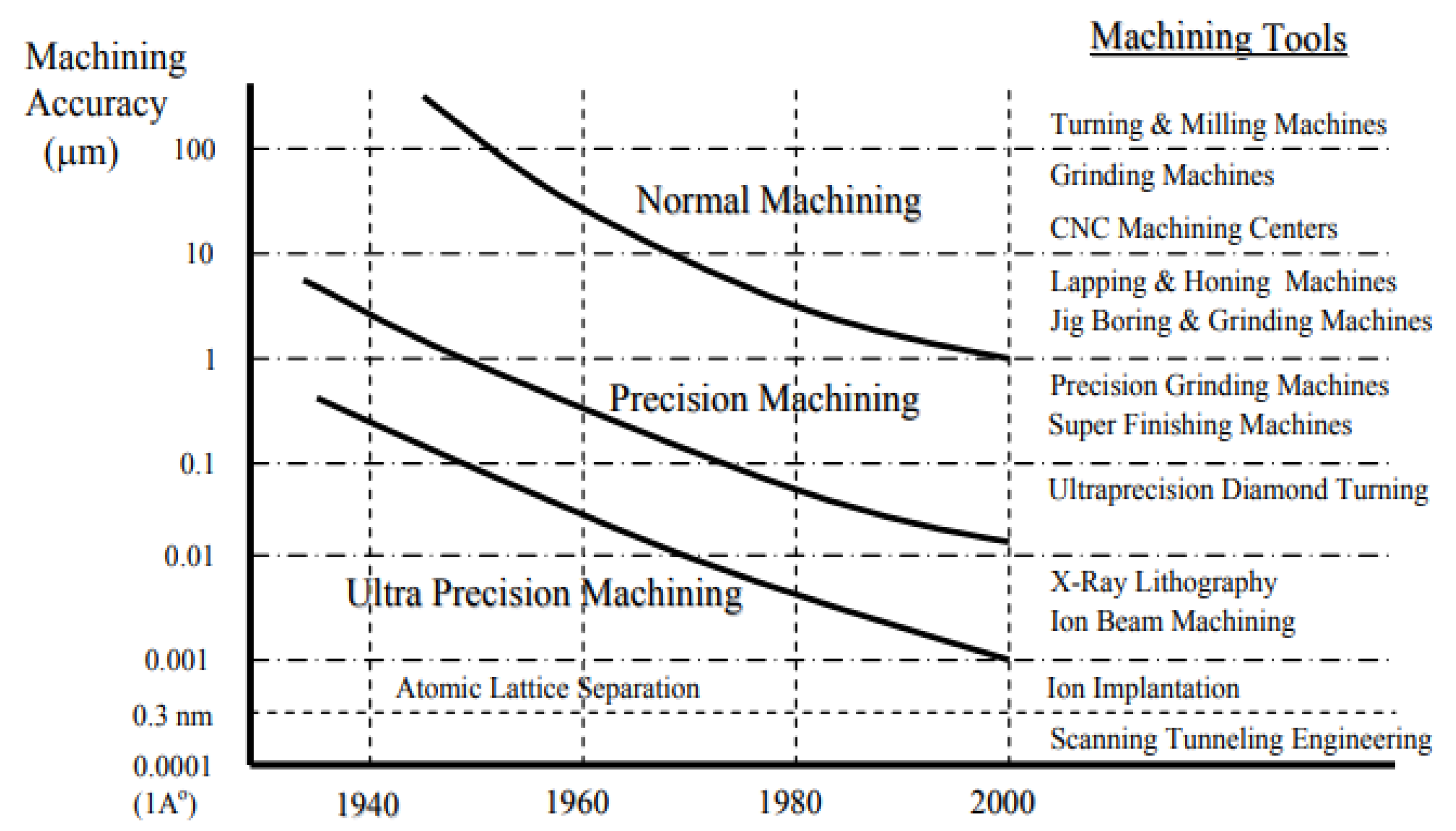
  27. Taniguchi, N. Current Status in, and Future Trends of, Ultraprecision Machining and Ultrafine Materials Processing. CIRP Ann. 1983, 32, 573–582. [Google Scholar] [CrossRef]
  28. Jain, V.K. Nanofinishing Science and Technology; CRC Press: Boca Raton, FL, USA, 2017. [Google Scholar]
  29. Chang, Y.-H.; Tsay, Y.-S.; Huang, C.-T.; Tseng’s, W.-L. The moisture buffering effect of finishing coatings on wooden materials. In Indoor Air; Blackwell Munksgaard: Ghent, Belgium, 2016. [Google Scholar]
  30. Kumar, M.; Alok, A.; Kumar, V.; Das, M. Advanced abrasive-based nano-finishing processes: Challenges, principles and recent applications. Mater. Manuf. Process. 2022, 37, 372–392. [Google Scholar] [CrossRef]
  31. Mori, Y.; Yamauchi, K.; Endo, K. Elastic emission machining. Precis. Eng. 1987, 9, 123–128. [Google Scholar] [CrossRef]
  32. Tian, Y.B.; Ang, Y.J.; Zhong, Z.W.; Xu, H.; Tan, R. Chemical Mechanical Polishing of Glass Disk Substrates: Preliminary Experimental Investigation. Mater. Manuf. Process. 2013, 28, 488–494. [Google Scholar] [CrossRef]
  33. Kathiresan, S.; Mohan, B. Experimental Analysis of Magneto Rheological Abrasive Flow Finishing Process on AISI Stainless steel 316L. Mater. Manuf. Process. 2018, 33, 422–432. [Google Scholar] [CrossRef]
  34. Das, M.; Jain, V.; Ghoshdastidar, P. Fluid flow analysis of magnetorheological abrasive flow finishing (MRAFF) process. Int. J. Mach. Tools Manuf. 2008, 48, 415–426. [Google Scholar] [CrossRef]
  35. Kumar, A.; Alam, Z.; Khan, D.A.; Jha, S. Nanofinishing of FDM-fabricated components using ball end magnetorheological finishing process. Mater. Manuf. Process. 2019, 34, 232–242. [Google Scholar] [CrossRef]
  36. Peng, C.; Fu, Y.; Wei, H.; Li, S.; Wang, X.; Gao, H. Study on Improvement of Surface Roughness and Induced Residual Stress for Additively Manufactured Metal Parts by Abrasive Flow Machining. Procedia CIRP 2018, 71, 386–389. [Google Scholar] [CrossRef]
  37. Guo, C.; Shi, Z.; Mullany, B.A.; Linke, B.S.; Yamaguchi, H.; Chaudhari, R.; Hucker, S.; Shih, A. Recent Advancements in Machining With Abrasives. J. Manuf. Sci. Eng. 2020, 142, 11. [Google Scholar] [CrossRef]
  38. Wan, S.; Ang, Y.J.; Sato, T.; Lim, G.C. Process modeling and CFD simulation of two-way abrasive flow machining. Int. J. Adv. Manuf. Technol. 2014, 71, 1077–1086. [Google Scholar] [CrossRef]
  39. Hamdi, H.; Valiorgue, F.; Mabrouki, T. Material Removal Processes by Cutting and Abrasion: Numerical Methodologies, Present Results and Insights. In Thermomechanical Industrial Processes; Bergheau, J.-M., Ed.; John Wiley & Sons, Inc.: Hoboken, NJ, USA, 2014; pp. 187–246. [Google Scholar] [CrossRef]
  40. Samoilenko, M.; Lanik, G.; Brailovski, V. Towards the Determination of Machining Allowances and Surface Roughness of 3D-Printed Parts Subjected to Abrasive Flow Machining. J. Manuf. Mater. Process. 2021, 5, 111. [Google Scholar] [CrossRef]
  41. Sankar, M.R.; Jain, V.K.; Ramkumar, J. Abrasive flow machining (AFM): An Overview. In Proceedings of the INDO-US Workshop on Smart Machine Tools, Intelligent Machining Systems and Multi-Scale Manufacturing, Tamil Nadu, India, 18 December 2008; p. 10. [Google Scholar]
  42. Li, J.; Sun, F.; Wei, L.; Zhang, X.; Xu, Y. The single factor experiment of the non-linear tube in abrasive flow machining. J. Meas. Eng. 2017, 5, 11–18. [Google Scholar] [CrossRef]
  43. Li, X.; Li, Q.; Ye, Z.; Zhang, Y.; Ye, M.; Wang, C. Surface Roughness Tuning at Sub-Nanometer Level by Considering the Normal Stress Field in Magnetorheological Finishing. Micromachines 2021, 12, 997. [Google Scholar] [CrossRef]
  44. Jackson, M.J. Recent advances in ultraprecision abrasive machining processes. SN Appl. Sci. 2020, 2, 7. [Google Scholar] [CrossRef]
  45. Kumari, C.; Chak, S.K. A review on magnetically assisted abrasive finishing and their critical process parameters. Manuf. Rev. 2018, 5, 13. [Google Scholar] [CrossRef]
  46. Sambharia, J.K.; Mali, H.S.; Garg, V. Experimental investigation on unidirectional abrasive flow machining of trim die workpiece. Mater. Manuf. Process. 2018, 33, 651–660. [Google Scholar] [CrossRef]
  47. Das, M.; Jain, V.K.; Ghoshdastidar, P.S. Analysis of magnetorheological abrasive flow finishing (MRAFF) process. Int. J. Adv. Manuf. Technol. 2008, 38, 613–621. [Google Scholar] [CrossRef]
  48. Chawla, G.; Mittal, V.K.; Mittal, S. Experimental Investigation of Process Parameters of Al-SiC-B4C MMCs Finished by a Novel Magnetic Abrasive Flow Machining Setup. Walailak J. Sci. Technol. 2021, 18, 18. [Google Scholar] [CrossRef]
  49. Bhardwaj, A.; Ali, P.; Walia, R.S.; Murtaza, Q.; Pandey, S.M. Development of Hybrid Forms of Abrasive Flow Machining Process: A Review. In Advances in Industrial and Production Engineering; Springer: Berlin/Heidelberg, Germany, 2019; pp. 41–67. [Google Scholar] [CrossRef]
  50. Gov, K.; Eyercioglu, O. Effects of abrasive types on the surface integrity of abrasive-flow-machined surfaces. Proc. Inst. Mech. Eng. Part B J. Eng. Manuf. 2016, 232, 1044–1053. [Google Scholar] [CrossRef]
  51. Tzeng, H.-J.; Yan, B.-H.; Hsu, R.-T.; Chow, H.-M. Finishing effect of abrasive flow machining on micro slit fabricated by wire-EDM. Int. J. Adv. Manuf. Technol. 2007, 34, 649–656. [Google Scholar] [CrossRef]
  52. Tzeng, H.-J.; Yan, B.-H.; Hsu, R.-T.; Lin, Y.-C. Self-modulating abrasive medium and its application to abrasive flow machining for finishing micro channel surfaces. Int. J. Adv. Manuf. Technol. 2007, 32, 1163–1169. [Google Scholar] [CrossRef]
  53. Ferchow, J.; Baumgartner, H.; Klahn, C.; Meboldt, M. Model of surface roughness and material removal using abrasive flow machining of selective laser melted channels. Rapid Prototyp. J. 2020, 26, 1165–1176. [Google Scholar] [CrossRef]
  54. Kumari, C.; Chak, S.K. Study on influential parameters of hybrid AFM processes: A review. Manuf. Rev. 2019, 6, 23. [Google Scholar] [CrossRef]
  55. Orbital and/or Reciprocal Machining with a Viscous Plastic Medium. 1 November 1989. Available online: https://patents.google.com/patent/CA2001970C/en (accessed on 18 January 2022).
  56. Xu, Y.C.; Zhang, K.H.; Lu, S.; Liu, Z.Q. Experimental Investigations into Abrasive Flow Machining of Helical Gear. Key Eng. Mater. 2013, 546, 65–69. [Google Scholar] [CrossRef]
  57. Dhull, S.; Mishra, R.; Walia, R.; Murtaza, Q.; Niranjan, M. Innovations in Different Abrasive Flow Machining Processes: A Review. J. Physics Conf. Ser. 2021, 1950, 012048. [Google Scholar] [CrossRef]
  58. Li, Y.; Ren, C.; Wang, H.; Hu, Y.; Ning, F.; Wang, X.; Cong, W. Edge surface grinding of CFRP composites using rotary ultrasonic machining: Comparison of two machining methods. Int. J. Adv. Manuf. Technol. 2019, 100, 3237–3248. [Google Scholar] [CrossRef]
  59. Wang, H.; Ning, F.; Hu, Y.; Cong, W. Surface grinding of CFRP composites using rotary ultrasonic machining: A comparison of workpiece machining orientations. Int. J. Adv. Manuf. Technol. 2018, 95, 2917–2930. [Google Scholar] [CrossRef]
  60. Wang, H.; Cong, W.; Ning, F.; Hu, Y. A study on the effects of machining variables in surface grinding of CFRP composites using rotary ultrasonic machining. Int. J. Adv. Manuf. Technol. 2018, 95, 3651–3663. [Google Scholar] [CrossRef]
  61. Dixit, N.; Sharma, V.; Kumar, P. Research trends in abrasive flow machining: A systematic review. J. Manuf. Process. 2021, 64, 1434–1461. [Google Scholar] [CrossRef]
  62. Ge, J.-Q.; Ren, Y.-L.; Xu, X.-S.; Li, C.; Li, Z.-A.; Xiang, W.-F. Numerical and experimental study on the ultrasonic-assisted soft abrasive flow polishing characteristics. Int. J. Adv. Manuf. Technol. 2021, 112, 3215–3233. [Google Scholar] [CrossRef]
  63. Wang, J.; Zhu, J.; Liew, P.J. Material Removal in Ultrasonic Abrasive Polishing of Additive Manufactured Components. Appl. Sci. 2019, 9, 5359. [Google Scholar] [CrossRef]
  64. Li, J.; Zhu, F.; Yu, J. An ultrasonic-assisted soft abrasive flow processing method for mold structured surfaces. Adv. Mech. Eng. 2019, 11, 1–17. [Google Scholar] [CrossRef]
  65. Wang, T.; Chen, D.; Zhang, W.; An, L. Study on key parameters of a new abrasive flow machining (AFM) process for surface finishing. Int. J. Adv. Manuf. Technol. 2019, 101, 39–54. [Google Scholar] [CrossRef]
  66. Walia, R.S.; Shan, H.; Kumar, P. Modelling of Centrifugal-Force-Assisted Abrasive Flow Machining. 2009. Available online: https://www.semanticscholar.org/paper/Modelling-of-centrifugal-force-assisted-abrasive-Walia-Shan/d191af51ec105ef9d349682af75a7cbaf0d7c109 (accessed on 21 November 2021).
  67. Bradley, C.; Wong, Y. Surface Texture Indicators of Tool Wear—A Machine Vision Approach. Int. J. Adv. Manuf. Technol. 2001, 17, 435–443. [Google Scholar] [CrossRef]
  68. Hashmi, A.W.; Mali, H.S.; Meena, A.; Khilji, I.A.; Chilakamarry, C.R.; Saffe, S.N.B.M. Experimental investigation on magnetorheological finishing process parameters. Mater. Today Proc. 2021, 48, 1892–1898. [Google Scholar] [CrossRef]
  69. Jha, S.; Jain, V.K. Design and development of the magnetorheological abrasive flow finishing (MRAFF) process. Int. J. Mach. Tools Manuf. 2004, 44, 1019–1029. [Google Scholar] [CrossRef]
  70. Sankar, M.R.; Taye, D.; Manohar, M.; Sarkar, D.; Basu, B. Nano Finishing of HDPE/Al2O3/HAp Ternary Composite Based Acetabular Socket using Polymer Rheological Abrasive Semisolid Medium. Int. J. Nanobiotechnology 2016, 2, 5–8. [Google Scholar]
  71. Ali, P.; Walia, R.S.; Murtaza, Q.; Singari, R. Material Removal Analysis of Hybrid EDM-Assisted Centrifugal Abrasive Flow Machining Process for Performance Enhancement. 2020. Available online: https://www.semanticscholar.org/paper/Material-removal-analysis-of-hybrid-EDM-assisted-Ali-Walia/fcf01761d2c2e7ac5db54cdfcc79025aa51855de (accessed on 21 November 2021).
  72. Brar, B.S.; Walia, R.S.; Singh, V.P. Electrochemical-aided abrasive flow machining (ECA2FM) process: A hybrid machining process. Int. J. Adv. Manuf. Technol. 2015, 79, 329–342. [Google Scholar] [CrossRef]
  73. Singh, S.; Sankar, M.R.; Jain, V.K.; Ramkumar, J. Modeling of Finishing Forces and Surface Roughness in Abrasive Flow Finishing (AFF) Process using Rheological Properties. In Proceedings of the 5th International & 26th All India Manufacturing Technology, Design and Research Conference (AIMTDR 2014), Assam, India, 12–14 December 2014; p. 6. [Google Scholar]
  74. Jayant, V.K.J. Analysis of finishing forces and surface finish during magnetorheological abrasive flow finishing of asymmetric workpieces. J. Micromanufacturing 2019, 2, 133–151. [Google Scholar] [CrossRef]
  75. Li, J.; Wang, L.; Zhang, H.; Hu, J.; Zhang, X.-M.; Zhao, W. Mechanism Research and Quality Discussion on Precision Machining of Fifth-Order Variable-Diameter Pipe by Abrasive Flow. 2020. Available online: https://www.semanticscholar.org/paper/Mechanism-Research-and-Quality-Discussion-on-of-by-Li-Wang/76744b89f28eb96660f0a5a4e306fbe985b2125f (accessed on 18 January 2022).
  76. Dabrowski, L.; Marciniak, M.; Szewczyk, T. Analysis of Abrasive Flow Machining with an Electrochemical Process Aid. Proc. Inst. Mech. Eng. Part B J. Eng. Manuf. 2006, 220, 397–403. [Google Scholar] [CrossRef]
  77. Kumar, S.S.; Hiremath, S.S. A Review on Abrasive Flow Machining (AFM). Procedia Technol. 2016, 25, 1297–1304. [Google Scholar] [CrossRef]
  78. Wang, X.; Williams, R.E.; Sealy, M.P.; Rao, P.K.; Guo, Y. Stochastic Modeling and Analysis of Spindle Power During Hard Milling With a Focus on Tool Wear. J. Manuf. Sci. Eng. 2018, 140, 111011. [Google Scholar] [CrossRef]
  79. Jain, N.K.; Jain, V.K.; Deb, K. Optimization of process parameters of mechanical type advanced machining processes using genetic algorithms. Int. J. Mach. Tools Manuf. 2007, 47, 900–919. [Google Scholar] [CrossRef]
  80. Dhull, S.; Murtaza, Q.; Walia, R.S.; Niranjan, M.S.; Vats, S. Abrasive Flow Machining Process Hybridization with Other Non-Traditional Machining Processes: A Review. In International Conference in Mechanical and Energy Technology; Springer: Singapore, 2020; pp. 101–109. [Google Scholar] [CrossRef]
  81. Vaishya, R.; Walia, R.; Kalra, P. Design and Development of Hybrid Electrochemical and Centrifugal Force Assisted Abrasive Flow Machining. Mater. Today Proc. 2015, 2, 3327–3341. [Google Scholar] [CrossRef]
  82. Uhlmann, E.; Roßkamp, S. Modelling of Material Removal in Abrasive Flow Machining. Int. J. Autom. Technol. 2018, 12, 883–891. [Google Scholar] [CrossRef]
  83. Guo, J.; Song, C.; Fu, Y.; Au, K.H.; Kum, C.W.; Goh, M.H.; Ren, T.; Huang, R.; Sun, C.-N. Internal Surface Quality Enhancement of Selective Laser Melted Inconel 718 by Abrasive Flow Machining. J. Manuf. Sci. Eng. 2020, 142, 101003. [Google Scholar] [CrossRef]
  84. Mali, H.S.; Prajwal, B.; Gupta, D.; Kishan, J. Abrasive flow finishing of FDM printed parts using a sustainable media. Rapid Prototyp. J. 2018, 24, 593–606. [Google Scholar] [CrossRef]
  85. Subramanian, K.T.; Balashanmugam, N.; Shashi Kumar, P.V. Nanometric finishing on biomedical implants by abrasive flow finishing. J. Inst. Eng. Ser. C 2016, 97, 55–61. [Google Scholar] [CrossRef]
  86. Kumar, S.; Jain, V.K.; Sidpara, A. Nanofinishing of freeform surfaces (knee joint implant) by rotational-magnetorheological abrasive flow finishing (R-MRAFF) process. Precis. Eng. 2015, 42, 165–178. [Google Scholar] [CrossRef]
  87. Yang, J.; Li, S.; Wang, Z.; Dong, H.; Wang, J.; Tang, S. Using Deep Learning to Detect Defects in Manufacturing: A Comprehensive Survey and Current Challenges. Materials 2020, 13, 5755. [Google Scholar] [CrossRef] [PubMed]
  88. Hashmi, A.W.; Mali, H.S.; Meena, A.; Puerta, V.; Kunkel, M.E. Surface characteristics improvement methods for metal additively manufactured parts: A review. Adv. Mater. Process. Technol. 2022, 1–40. [Google Scholar] [CrossRef]
  89. Hashmi, A.W.; Mali, H.S.; Meena, A. Improving the surface characteristics of additively manufactured parts: A review. Mater. Today Proc. 2021, in press. [Google Scholar] [CrossRef]
  90. Hashmi, A.W.; Mali, H.S.; Meena, A. The Surface Quality Improvement Methods for FDM Printed Parts: A Review. Mater. Form. Mach. Tribol. 2021, 167–194. [Google Scholar] [CrossRef]
  91. Hashmi, A.W.; Mali, H.S.; Meena, A. Surface quality improvement methods of additively manufactured parts: A review. Solid State Technol. 2020, 63, 23477–23517. [Google Scholar]
  92. Hashmi, A.W.; Mali, H.S.; Meena, A.; Khilji, I.A.; Hashmi, M.F.; Saffe, S.N.B.M. Machine vision for the measurement of machining parameters: A review. Mater. Today Proc. 2021, 56, 1939–1946. [Google Scholar] [CrossRef]
  93. Hashmi, A.W.; Mali, H.S.; Meena, A.; Khilji, I.A.; Hashmi, M.F.; Saffe, S.N.B.M. Artificial intelligence techniques for implementation of intelligent machining. Mater. Today Proc. 2022, 56, 1947–1955. [Google Scholar] [CrossRef]
  94. Hashmi, A.W.; Mali, H.S.; Meena, A. Experimental investigation on abrasive flow Machining (AFM) of FDM printed hollow truncated cone parts. Mater. Today Proc. 2022, 56, 1369–1375. [Google Scholar] [CrossRef]
  95. Hashmi, A.W.; Mali, H.S.; Meena, A. Design and fabrication of a low-cost one-way abrasive flow finishing set-up using 3D printed parts. Mater. Today Proc. 2022, 62, 7554–7563. [Google Scholar] [CrossRef]
  96. Hashmi, A.W.; Mali, H.S.; Meena, A.; Saxena, K.K.; Puerta, A.P.V.; Buddhi, D. A newly developed coal-ash-based AFM media characterization for abrasive flow finishing of FDM printed hemispherical ball shape. Int. J. Interact. Des. Manuf. 2022, 1–16. [Google Scholar] [CrossRef]
  97. Hashmi, A.W.; Mali, H.S.; Meena, A. Experimental investigation of an innovative viscometer for measuring the viscosity of Ferrofluid. Mater. Today Proc. 2022, 50, 2037–2043. [Google Scholar] [CrossRef]
  98. Fu, Y.; Gao, H.; Wang, X.; Guo, D. Machining the integral impeller and blisk of aero-engines: A review of surface finishing and strengthening technologies. Chin. J. Mech. Eng. 2017, 30, 528–543. [Google Scholar] [CrossRef]
  99. Hiremath, S.S. Effect of surface roughness and surface topography on wettability of machined biomaterials using flexible viscoelastic polymer abrasive media. Surf. Topogr. Metrol. Prop. 2019, 7, 015004. [Google Scholar]
  100. Petare, A.C.; Mishra, A.; Palani, I.A.; Jain, N.K. Study of laser texturing assisted abrasive flow finishing for enhancing surface quality and microgeometry of spur gears. Int. J. Adv. Manuf. Technol. 2019, 101, 785–799. [Google Scholar] [CrossRef]
  101. Singh, S.; Sankar, M.R. Rheological study of the developed medium and its correlation with surface roughness during abrasive flow finishing of micro-slots. Mach. Sci. Technol. 2020, 24, 882–905. [Google Scholar] [CrossRef]
  102. Singh, P.; Singh, L.; Singh, S. Analyzing process parameters for finishing of small holes using magnetically assisted abrasive flow machining process. J. Bio-Tribo-Corros. 2020, 6, 17. [Google Scholar] [CrossRef]
  103. Mohammadian, N.; Turenne, S.; Brailovski, V. Surface finish control of additively-manufactured Inconel 625 components using combined chemical-abrasive flow polishing. J. Mater. Processing Technol. 2018, 252, 728–738. [Google Scholar] [CrossRef]
  104. Uhlmann, E.; Schmiedel, C.; Wendler, J. CFD Simulation of the Abrasive Flow Machining Process. Procedia CIRP 2015, 31, 209–214. [Google Scholar] [CrossRef]
  105. Das, M.; Jain, V.K.; Ghoshdastidar, P. A 2D CFD simulation of MR polishing medium in magnetic field-assisted finishing process using electromagnet. Int. J. Adv. Manuf. Technol. 2015, 76, 173–187. [Google Scholar] [CrossRef]
  106. Jain, K.; Jain, V.K. Stochastic simulation of active grain density in abrasive flow machining. J. Mater. Process. Technol. 2004, 1, 17–22. [Google Scholar] [CrossRef]
  107. Williams, R.E.; Rajurkar, K.P. Stochastic Modeling and Analysis of Abrasive Flow Machining. J. Eng. Ind. 1992, 114, 74–81. [Google Scholar] [CrossRef]
  108. Dash, R.; Maity, K. Simulation of abrasive flow machining process for 2D and 3D mixture models. Front. Mech. Eng. 2015, 10, 424–432. [Google Scholar] [CrossRef]
  109. Sambharia, J.; Mali, H.S. Recent developments in abrasive flow finishing process: A review of current research and future prospects. Proc. Inst. Mech. Eng. Part B J. Eng. Manuf. 2019, 233, 388–399. [Google Scholar] [CrossRef]
  110. Petare, A.C.; Jain, N.K. A critical review of past research and advances in abrasive flow finishing process. Int. J. Adv. Manuf. Technol. 2018, 97, 741–782. [Google Scholar] [CrossRef]
  111. Chih-Hua, W.; Wai, K.C.; Ming, W.S.Y.; Muhammad, A.B.A. Numerical and experimental investigation of abrasive flow machining of branching channels. Int. J. Adv. Manuf. Technol. 2020, 108, 2945–2966. [Google Scholar] [CrossRef]
  112. Fu, Y.; Wang, X.; Gao, H.; Wei, H.; Li, S. Blade surface uniformity of blisk finished by abrasive flow machining. Int. J. Adv. Manuf. Technol. 2016, 84, 1725–1735. [Google Scholar] [CrossRef]
  113. Shen, R.; Jiao, Z.; Parker, T.; Sun, Y.; Wang, Q. Recent application of Computational Fluid Dynamics (CFD) in process safety and loss prevention: A review. J. Loss Prev. Process Ind. 2020, 67, 104252. [Google Scholar] [CrossRef]
  114. Matko, T.; Chew, J.; Wenk, J.; Chang, J.; Hofman, J. Computational fluid dynamics simulation of two-phase flow and dissolved oxygen in a wastewater treatment oxidation ditch. Process Saf. Environ. Prot. 2021, 145, 340–353. [Google Scholar] [CrossRef]
  115. Badshah, M.; Badshah, S.; Jan, S. Comparison of computational fluid dynamics and fluid structure interaction models for the performance prediction of tidal current turbines. J. Ocean Eng. Sci. 2020, 5, 164–172. [Google Scholar] [CrossRef]
  116. Maity, K.P.; Dash, R. Modelling of Material Removal in Abrasive Flow Machining Process Using CFD simulation. J. Basic Appl. Eng. Res. 2014, 2, 73–78. [Google Scholar]
  117. Jeon, D.H. Computational fluid dynamics simulation of anode-supported solid oxide fuel cells with implementing complete overpotential model. Energy 2019, 188, 116050. [Google Scholar] [CrossRef]
  118. Yang, J. Computational fluid dynamics studies on the induction period of crude oil fouling in a heat exchanger tube. Int. J. Heat Mass Transf. 2020, 159, 120129. [Google Scholar] [CrossRef]
  119. Baraiya, R.; Babbar, A.; Jain, V.; Gupta, D. In-situ simultaneous surface finishing using abrasive flow machining via novel fixture. J. Manuf. Process. 2020, 50, 266–278. [Google Scholar] [CrossRef]
  120. Melendez, J.; Reilly, D.; Duran, C. Numerical investigation of ventilation efficiency in a Combat Arms training facility using computational fluid dynamics modelling. Build. Environ. 2020, 188, 107404. [Google Scholar] [CrossRef]
  121. Comminal, R.; da Silva, W.R.L.; Andersen, T.J.; Stang, H.; Spangenberg, J. Modelling of 3D concrete printing based on computational fluid dynamics. Cem. Concr. Res. 2020, 138, 106256. [Google Scholar] [CrossRef]
  122. Gudipadu, V.; Sharma, A.K.; Singh, N. Simulation of media behaviour in vibration assisted abrasive flow machining. Simul. Model. Pr. Theory 2015, 51, 1–13. [Google Scholar] [CrossRef]
  123. Kim, K.J.; Kim, Y.G.; Kim, K.H. Characterization of deburring by abrasive flow machining for AL6061. Appl. Sci. 2022, 12, 2048. [Google Scholar] [CrossRef]
  124. Fu, Y.; Gao, H.; Yan, Q.; Wang, X.; Wang, X. Rheological characterisation of abrasive media and finishing behaviours in abrasive flow machining. Int. J. Adv. Manuf. Technol. 2020, 107, 3569–3580. [Google Scholar] [CrossRef]
  125. Pradhan, S.; Das, S.R.; Jena, P.C.; Dhupal, D. Machining performance evaluation under recently developed sustainable HAJM process of zirconia ceramic using hot SiC abrasives: An experimental and simulation approach. Proc. Inst. Mech. Eng. Part C: J. Mech. Eng. Sci. 2022, 236, 1009–1035. [Google Scholar] [CrossRef]
  126. Pradhan, S.; Dhupal, D.; Das, S.R.; Jena, P.C. Experimental investigation and optimization on machined surface of Si3N4 ceramic using hot SiC abrasive in HAJM. Mater. Today Proc. 2021, 44, 1877–1887. [Google Scholar] [CrossRef]
  127. Amar, A.K.; Tandon, P. Investigation of gelatin enabled abrasive water slurry jet machining (AWSJM). CIRP J. Manuf. Sci. Technol. 2021, 33, 1–14. [Google Scholar] [CrossRef]
  128. Zou, T.; Yan, Q.; Wang, L.; An, Y.; Qu, J.; Li, J. Research on quality control of precision machining straight internal gear by abrasive flow based on large eddy simulation. Int. J. Adv. Manuf. Technol. 2022, 119, 5315–5334. [Google Scholar] [CrossRef]
  129. Chen, C.; Liu, Y.; Tang, J.; Zhang, H. Effect of nozzle pressure ratios on the flow and distribution of abrasive particles in abrasive air jet machining. Powder Technol. 2022, 397, 117114. [Google Scholar] [CrossRef]
  130. Zhang, B.-C.; Chen, S.-F.; Khiabani, N.; Qiao, Y.; Wang, X.-C. Research on the underlying mechanism behind abrasive flow machining on micro-slit structures and simulation of viscoelastic media. Adv. Manuf. 2022, 1–15. [Google Scholar] [CrossRef]
  131. Zhang, B.; Qiao, Y.; Khiabani, N.; Wang, X. Study on rheological behaviors of media and material removal mechanism for abrasive flow machining (AFM) micro structures and corresponding simulations. J. Manuf. Process. 2021, 73, 248–259. [Google Scholar] [CrossRef]
  132. Zhang, B.; Chen, S.; Wang, X. Machining uniformity and property change of abrasive media for micro-porous structures. J. Mater. Process. Technol. 2022, 307, 117675. [Google Scholar] [CrossRef]
  133. Zhu, G.; Li, H.; Wang, Z.; Zhang, T.; Liu, M. Semi-resolved CFD-DEM modeling of gas-particle two-phase flow in the micro-abrasive air jet machining. Powder Technol. 2021, 381, 585–600. [Google Scholar] [CrossRef]
  134. Gautam, S.; Neopane, H.P.; Acharya, N.; Chitrakar, S.; Thapa, B.S.; Zhu, B. Sediment erosion in low specific speed francis turbines: A case study on effects and causes. Wear 2020, 442–443, 203152. [Google Scholar] [CrossRef]
  135. Jain, V.K.; Kumar, R.; Dixit, P.M.; Sidpara, A. Investigations into abrasive flow finishing of complex workpieces using FEM. Wear 2009, 267, 71–80. [Google Scholar] [CrossRef]
  136. Singh, S.; Shan, H. Development of magneto abrasive flow machining process. Int. J. Mach. Tools Manuf. 2002, 42, 953–959. [Google Scholar] [CrossRef]
  137. Dong, Z.; Ya, G.; Liu, J. Study on machining mechanism of high viscoelastic abrasive flow machining for surface finishing. Proc. Inst. Mech. Eng. Part B J. Eng. Manuf. 2015, 231, 608–617. [Google Scholar] [CrossRef]
  138. Bhaumik, M.; Maity, K. Finite element simulation and experimental investigation of Ti-5Al-2.5Sn titanium alloy during EDM process. Mater. Today Proc. 2020, 46, 24–29. [Google Scholar] [CrossRef]
  139. Santana, M.; Arnouts, L.; Massart, T.; Gonçalves, P.; Berke, P. Corotational 3D joint finite element tailored for the simulation of bistable deployable structures. Eng. Struct. 2021, 227, 111387. [Google Scholar] [CrossRef]
  140. Bachini, E.; Farthing, M.W.; Putti, M. Intrinsic finite element method for advection-diffusion-reaction equations on surfaces. J. Comput. Phys. 2021, 424, 109827. [Google Scholar] [CrossRef]
  141. Kumar, N.; Shukla, M. Finite element analysis of multi-particle impact on erosion in abrasive water jet machining of titanium alloy. J. Comput. Appl. Math. 2012, 18, 4600–4610. [Google Scholar] [CrossRef]
  142. Pradhan, K.K.; Chakraverty, S. Finite Element Method. Comput. Struct. Mech. Sl 2019, 25–28. [Google Scholar] [CrossRef]
  143. Feng, Y.; Jianming, W.; Feihong, L. Numerical Simulation of Single Particle Acceleration Process by SPH Coupled FEM for Abrasive Waterjet Cutting. 2012. Available online: https://www.semanticscholar.org/paper/Numerical-simulation-of-single-particle-process-by-Feng-Jianming/5d8dce0cd48bf2defaf2da2167a8229748ab1ef5 (accessed on 18 January 2022).
  144. Jayswal, S.; Jain, V.; Dixit, P.M. Modeling and Simulation of Magnetic Abrasive Finishing Process. 2005. Available online: https://www.semanticscholar.org/paper/Modeling-and-simulation-of-magnetic-abrasive-Jayswal-Jain/9446cc873adb5351697b47c2b33b24d1db4071e1 (accessed on 18 January 2022).
  145. Kumar, G.; Yadav, V. Temperature distribution in the workpiece due to plane magnetic abrasive finishing using FEM. Int. J. Adv. Manuf. Technol. 2009, 41, 1051–1058. [Google Scholar] [CrossRef]
  146. Wang, J. Abrasive Waterjet Machining Simulation by Coupling Smoothed Particle Hydrodynamics/Finite Element Method. Chin. J. Mech. Eng. 2010, 5, 568. [Google Scholar] [CrossRef]
  147. Chaieb, I.; Moussa, N.B.; Fredj, N.B.; Salah, N.B. An Innovative Contactless Finite Element Simulation of the Shot Peening Process. 2021. Available online: https://www.semanticscholar.org/paper/An-innovative-contactless-finite-element-simulation-Chaieb-Moussa/d54db76880c4c80623386b586a91d50222726467 (accessed on 18 January 2022).
  148. Woytowitz, P.; Richman, R. Modeling of Damage from Multiple Impacts by Spherical Particles. 1999. Available online: https://www.semanticscholar.org/paper/Modeling-of-damage-from-multiple-impacts-by-Woytowitz-Richman/776daf54b2d273b24cfa2624d352f94db23d00ac (accessed on 18 January 2022).
  149. ElTobgy, M.S.; Ng, E.; Elbestawi, M. Finite Element Modeling of Erosive Wear. 2005. Available online: https://www.semanticscholar.org/paper/Finite-element-modeling-of-erosive-wear-ElTobgy-Ng/54ea117af8a21fec9804dc6414bac5950ebc53f2 (accessed on 18 January 2022).
  150. Junkar, M.; Jurisevic, B.; Fajdiga, M.; Grah, M. Finite Element Analysis of Single-Particle Impact in Abrasive Water Jet Machining. 2006. Available online: https://www.semanticscholar.org/paper/FINITE-ELEMENT-ANALYSIS-OF-SINGLE-PARTICLE-IMPACT-Junkar-Jurisevic/1b19697359a88f2ef142fb7069433bd57182e4cf (accessed on 18 January 2022).
  151. Amoo, O.; Oyewola, M.; Fagbenle, R. Application of the finite-element method to the solution of nonsimilar boundary layer-derived infinite series equations. Int. J. Heat Mass Transf. 2020, 161, 120244. [Google Scholar] [CrossRef]
  152. Singh, T.B.; Chohan, J.S.; Kumar, R. Performance analysis of vapour finishing apparatus for surface enhancement of FDM parts. Mater. Today Proc. 2020, 26, 3497–3502. [Google Scholar] [CrossRef]
  153. Zhang, T.; Zhou, X.; Liu, X. Reliability analysis of slopes using the improved stochastic response surface methods with multicollinearity. Eng. Geol. 2020, 271, 105617. [Google Scholar] [CrossRef]
  154. Zhao, Y.; Jiang, J.; Zhou, L.; Dai, Y.; Ni, F. Meso-structure image pre-selection method for two-dimensional finite element modeling in beam bending simulation of asphalt mixture. Constr. Build. Mater. 2021, 268, 121129. [Google Scholar] [CrossRef]
  155. Kim, Y.T.; Lee, M.J.; Lee, B.C. Simulation of adhesive joints using the superimposed finite element method and a cohesive zone model. Int. J. Adhes. Adhes. 2011, 31, 357–362. [Google Scholar] [CrossRef]
  156. Weiland, J. Analysis of back-face strain measurement for adhesively bonded single lap joints using strain gauge, Digital Image Correlation and finite element method. Int. J. Adhes. Adhes. 2020, 79, 102491. [Google Scholar] [CrossRef]
  157. Misra, A.; Pandey, P.M.; Dixit, U. Modeling and simulation of surface roughness in ultrasonic assisted magnetic abrasive finishing process. Int. J. Mech. Sci. 2017, 133, 344–356. [Google Scholar] [CrossRef]
  158. Judal, K.; Yadava, V. Modeling and simulation of cylindrical electro-chemical magnetic abrasive machining of AISI-420 magnetic steel. J. Mater. Process. Technol. 2013, 213, 2089–2100. [Google Scholar] [CrossRef]
  159. Tang, H.; Yang, W.; Liu, W.; Ma, J.; Luo, X. Characteristic of fixed abrasive polishing for fused silica in anhydrous environment. Optik 2020, 202, 163623. [Google Scholar] [CrossRef]
  160. Zhang, J.; Yang, X.; Sagar, S.; Dube, T.; Koo, D.D.; Kim, B.-G.; Jung, Y.-G. Smoothed Particle Hydrodynamics Modeling of Thermal Barrier Coating Removal Process Using Abrasive Water Jet Technique. J. Manuf. Sci. Eng. 2022, 1–22. [Google Scholar] [CrossRef]
  161. Ozcan, Y.; Tunc, L.T.; Kopacka, J.; Cetin, B.; Sulitka, M. Modelling and simulation of controlled depth abrasive water jet machining (AWJM) for roughing passes of free-form surfaces. Int. J. Adv. Manuf. Technol. 2021, 114, 3581–3596. [Google Scholar] [CrossRef]
  162. Liu, Y.; Zhao, Y.; Yoshigoe, K.; Zhang, S.; Chen, M. Simulating a high-speed abrasive particle impacting on a tensile block using SPH-FEM. Int. J. Adv. Manuf. Technol. 2021, 116, 2835–2845. [Google Scholar] [CrossRef]
  163. Du, M.; Wang, H.; Dong, H.; Guo, Y.; Ke, Y. Numerical research on multi-particle movements and nozzle wear involved in abrasive waterjet machining. Int. J. Adv. Manuf. Technol. 2021, 117, 2845–2858. [Google Scholar] [CrossRef]
  164. Vasudevan, B.; Natarajan, Y.; Kumar, R.P.; Chandra, K.U.; Sikder, D. Simulation of AWJ drilling process using the FEA coupled SPH models: A preliminary study. Mater. Today Proc. 2022, 62, 6022–6028. [Google Scholar] [CrossRef]
  165. Beigmoradi, S.; Vahdati, M. Experimental and numerical study of polishing of 2024 aluminum alloy using acoustics energy. J. Manuf. Process. 2022, 73, 440–453. [Google Scholar] [CrossRef]
  166. Klocke, F.; Soo, S.L.; Karpuschewski, B.; Webster, J.A.; Novovic, D.; Elfizy, A.; Axinte, D.A.; Tönissen, S. Abrasive machining of advanced aerospace alloys and composites. CIRP Ann. 2015, 64, 581–604. [Google Scholar] [CrossRef]
  167. Walia, R.S.; Shan, H.S.; Kumar, P.K. Finite element analysis of media used in the centrifugal force assisted abrasive flow machining process. Proc. Inst. Mech. Eng. Part B J. Eng. Manuf. 2006, 220, 1775–1785. [Google Scholar] [CrossRef]
  168. Yu, W.; Feng, Q.; Zu Ren, C. 3D Finite Element Analysis of Pile-up Formation in Abrasive Machining at Low Speed. Solid State Phenom. 2011, 175, 211–214. [Google Scholar] [CrossRef]
  169. Zhu, H.P.; Zhou, Z.Y.; Yang, R.Y.; Yu, A.B. Discrete particle simulation of particulate systems: Theoretical developments. Chem. Eng. Sci. 2007, 62, 3378–3396. [Google Scholar] [CrossRef]
  170. Xia, R.; Wang, X.; Li, B.; Wei, X.; Yang, Z. Discrete Element Method- (DEM-) Based Study on the Wear Mechanism and Wear Regularity in Scraper Conveyor Chutes. Math. Probl. Eng. 2019, 2019, 4191570. [Google Scholar] [CrossRef]
  171. Dranishnykov, S.; Dosta, M. Advanced approach for simulation results saving from discrete element method. Adv. Eng. Softw. 2019, 136, 102694. [Google Scholar] [CrossRef]
  172. Zhang, X.; Li, J.; Hu, J.; Zhao, W. The research of polishing nozzle quality based on discrete element method. J. Meas. Eng. 2017, 5, 29–39. [Google Scholar] [CrossRef]
  173. Yazarlu, A.; Dehestani, M. Application of discrete element method (DEM) in characterization of bond-slip behavior in RC beams with confinement subjected to corrosion. Structures 2020, 28, 1965–1976. [Google Scholar] [CrossRef]
  174. Rojas, E.; Vergara, V.; Soto, R. Case study: Discrete element modeling of wear in mining hoppers. Wear 2019, 430–431, 120–125. [Google Scholar] [CrossRef]
  175. Leonard, B.D.; Ghosh, A.; Sadeghi, F.; Shinde, S.; Mittelbach, M. Third body modeling in fretting using the combined finite-discrete element method. Int. J. Solids Struct. 2020, 51, 1375–1389. [Google Scholar] [CrossRef]
  176. Nutto, C.; Bierwisch, C.; Lagger, H.; Moseler, M.; Höhn, S.; Bremerstein, T.; Potthoff, A. Towards simulation of abrasive flow machining. In Proceedings of the 7th International Spheric Workshop, Prato, Italy, 29–30 May 2012. [Google Scholar]
  177. Xiu, T.-X.; Wang, W.; Liu, K.; Wang, Z.-Y.; Wei, D.-Z. Characteristics of force chains in frictional interface during abrasive flow machining based on discrete element method. Adv. Manuf. 2018, 6, 355–375. [Google Scholar] [CrossRef]
  178. Suehr, Q.J.; Marks, B.P.; Ryser, E.T.; Jeong, S. Modeling the Propagation of Salmonella within Bulk Almond Using Discrete Element Method Particle Simulation Technique. J. Food Eng. 2021, 293, 110363. [Google Scholar] [CrossRef]
  179. Peng, Z.; Doroodchi, E.; Moghtaderi, B. Heat transfer modelling in Discrete Element Method (DEM)-based simulations of thermal processes: Theory and model development. Prog. Energy Combust. Sci. 2020, 79, 100847. [Google Scholar] [CrossRef]
  180. Tsunazawa, Y.; Fujihashi, D.; Fukui, S.; Sakai, M.; Tokoro, C. Contact force model including the liquid-bridge force for wet-particle simulation using the discrete element method. Adv. Powder Technol. 2016, 27, 652–660. [Google Scholar] [CrossRef]
  181. Shih, A.J.; Denkena, B.; Grove, T.; Curry, D.; Hocheng, H.; Tsai, H.-Y.; Ohmori, H.; Katahira, K.; Pei, Z. Fixed abrasive machining of non-metallic materials. CIRP Ann. 2018, 67, 767–790. [Google Scholar] [CrossRef]
  182. Beigmoradi, S.; Vahdati, M. Investigation of vibratory bed effect on abrasive drag finishing: A DEM study. World J. Eng. 2021. [Google Scholar] [CrossRef]
  183. Ge, M.; Ji, S.; Tan, D.; Cao, H. Erosion analysis and experimental research of gas-liquid-solid soft abrasive flow polishing based on cavitation effects. Int. J. Adv. Manuf. Technol. 2021, 114, 3419–3436. [Google Scholar] [CrossRef]
  184. Huang, S.; Tang, Z.; Huang, J.; Ou, C.; Hui, Z. Investigation of influencing factors of wear in a sandblasting machine by CFD-DEM coupling. Part. Sci. Technol. 2021, 24, 1–10. [Google Scholar] [CrossRef]
  185. Zhu, G.; Li, H.; Zhang, T.; Liu, M. Modeling and simulation of micro-hole fabrication on brittle material using abrasive air jet machining. J. Manuf. Process. 2021, 72, 361–374. [Google Scholar] [CrossRef]
  186. Blaineau, P.; André, D.; Laheurte, R.; Darnis, P.; Darbois, N.; Cahuc, O.; Neauport, J. Subsurface mechanical damage during bound abrasive grinding of fused silica glass. Appl. Surf. Sci. 2015, 353, 764–773. [Google Scholar] [CrossRef]
  187. Ranjan, P.; Balasubramaniam, R.; Jain, V. Molecular Dynamics Simulation of Mechanical Polishing on Stainless Steel Using Diamond Nanoparticles. J. Manuf. Sci. Eng. 2018, 141, 014504. [Google Scholar] [CrossRef]
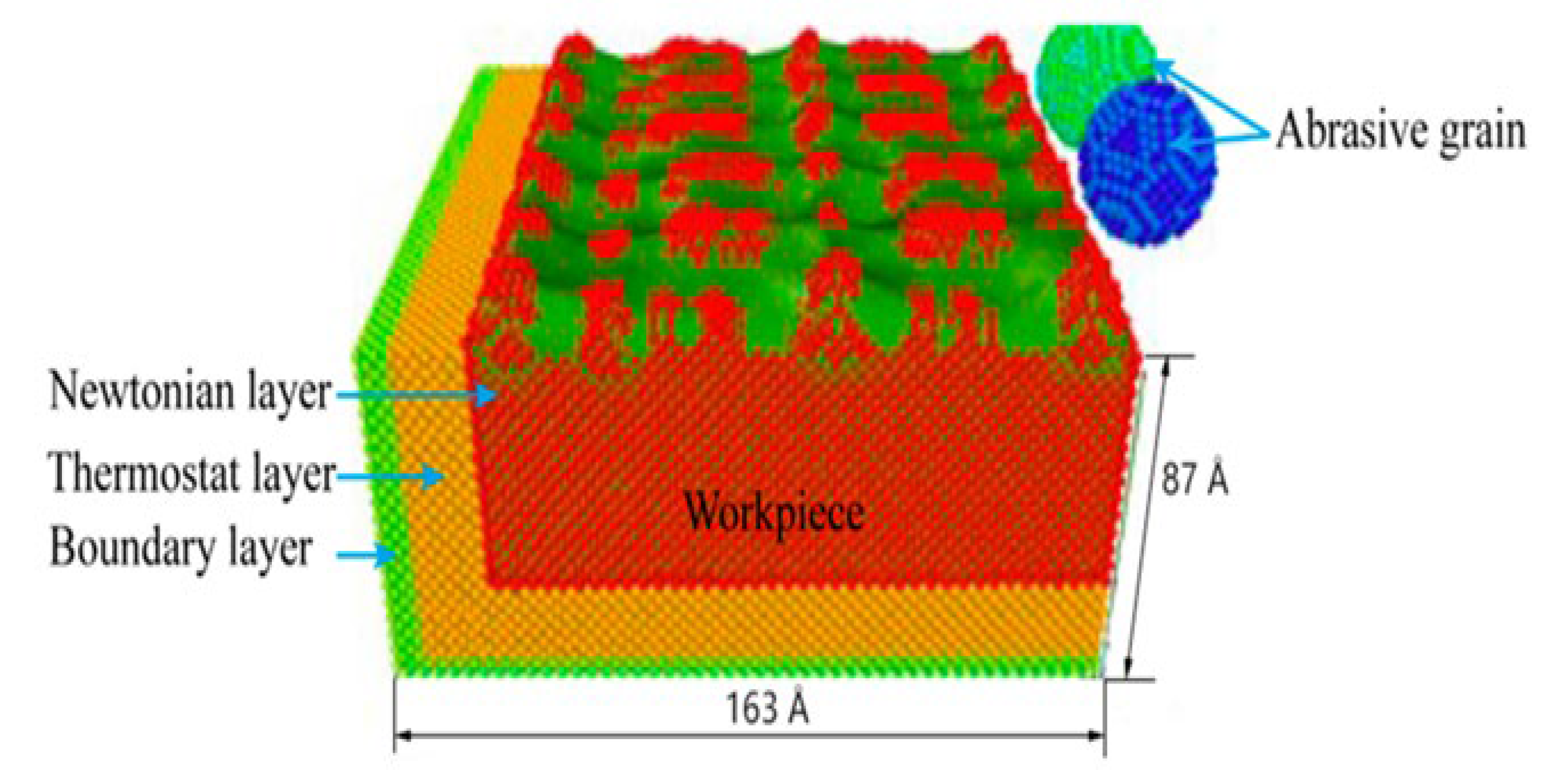
  188. Liu, Y.; Li, B.; Kong, L. A molecular dynamics investigation into nanoscale scratching mechanism of polycrystalline silicon carbide. Comput. Mater. Sci. 2018, 148, 76–86. [Google Scholar] [CrossRef]
  189. Liu, Y.; Li, B.; Kong, L. Molecular dynamics simulation of silicon carbide nanoscale material removal behavior. Ceram. Int. 2018, 44, 11910–11913. [Google Scholar] [CrossRef]
  190. Olufayo, O.; Abou-El-Hossein, K. Molecular Dynamics Modeling of Nanoscale Machining of Silicon. Procedia CIRP 2013, 8, 504–509. [Google Scholar] [CrossRef]
  191. Olufayo, O.; Otieno, T.; Akinlabi, E. Optimization Strategy for Milling of Copper Using Molecular Dynamics Modelling. Procedia Manuf. 2017, 7, 374–386. [Google Scholar] [CrossRef]
  192. James, S.; Sundaram, M. A molecular dynamics study of the effect of impact velocity, particle size and angle of impact of abrasive grain in the Vibration Assisted Nano Impact-machining by Loose Abrasives. Wear 2013, 303, 510–518. [Google Scholar] [CrossRef]
  193. Xu, J.; Li, J.; Zhu, P.; Li, B.; Zhao, C. Coarse-grained molecular dynamics simulations of particle behaviors in magnetorheological polishing fluid. Comput. Mater. Sci. 2019, 163, 68–81. [Google Scholar] [CrossRef]
  194. Wang, Y.; Tang, S.; Guo, J. Molecular dynamics study on deformation behaviour of monocrystalline GaN during nano abrasive machining. Appl. Surf. Sci. 2020, 510, 145492. [Google Scholar] [CrossRef]
  195. Yuan, S.; Guo, X.; Huang, J.; Gou, Y.; Jin, Z.; Kang, R.; Guo, D. Insight into the mechanism of low friction and wear during the chemical mechanical polishing process of diamond: A reactive molecular dynamics simulation. Tribol. Int. 2020, 148, 106308. [Google Scholar] [CrossRef]
  196. Parvandar Asadollahi, B.; Pour Panah, M.; Javdani, A. Experimental Investigation and Molecular Dynamics Simulation of Contributing Variables on Abrasive Water Jet on Aluminum Alloy 7075 Reinforced with Al2O3, Graphite and Silicon Carbide. Arab. J. Sci. Eng. 2022, 1–9. [Google Scholar] [CrossRef]
  197. Meng, X.; Yue, H.; Wu, W.; Dai, H. Simulation of abrasive polishing process of single crystal silicon based on molecular dynamics. Int. J. Adv. Manuf. Technol. 2022, 1–7. [Google Scholar] [CrossRef]
  198. Zhou, F.; Xu, J.; Ren, W.; Yu, P.; Yu, H. Research on mechanism of ultrasonic-assisted nano-cutting of sapphire based on molecular dynamics. Mech. Adv. Mater. Struct. 2022, 1–15. [Google Scholar] [CrossRef]
  199. Ranjan, P.; Owhal, A.; Chakrabarti, D.; Belgamwar, S.U.; Roy, T.; Balasubramaniam, R. Fundamental insights of mechanical polishing on polycrystalline Cu through molecular dynamics simulations. Mater. Today Commun. 2022, 32, 103980. [Google Scholar] [CrossRef]
  200. Su, Z.; Liang, Z.; Du, Y.; Zhou, H.; Ma, Y.; Qiu, T.; Zhao, B.; Zhou, T.; Wang, X. Cutting characteristics of monocrystalline silicon in elliptical vibration nano-cutting using molecular dynamics method. Comput. Mater. Sci. 2022, 212, 111589. [Google Scholar] [CrossRef]
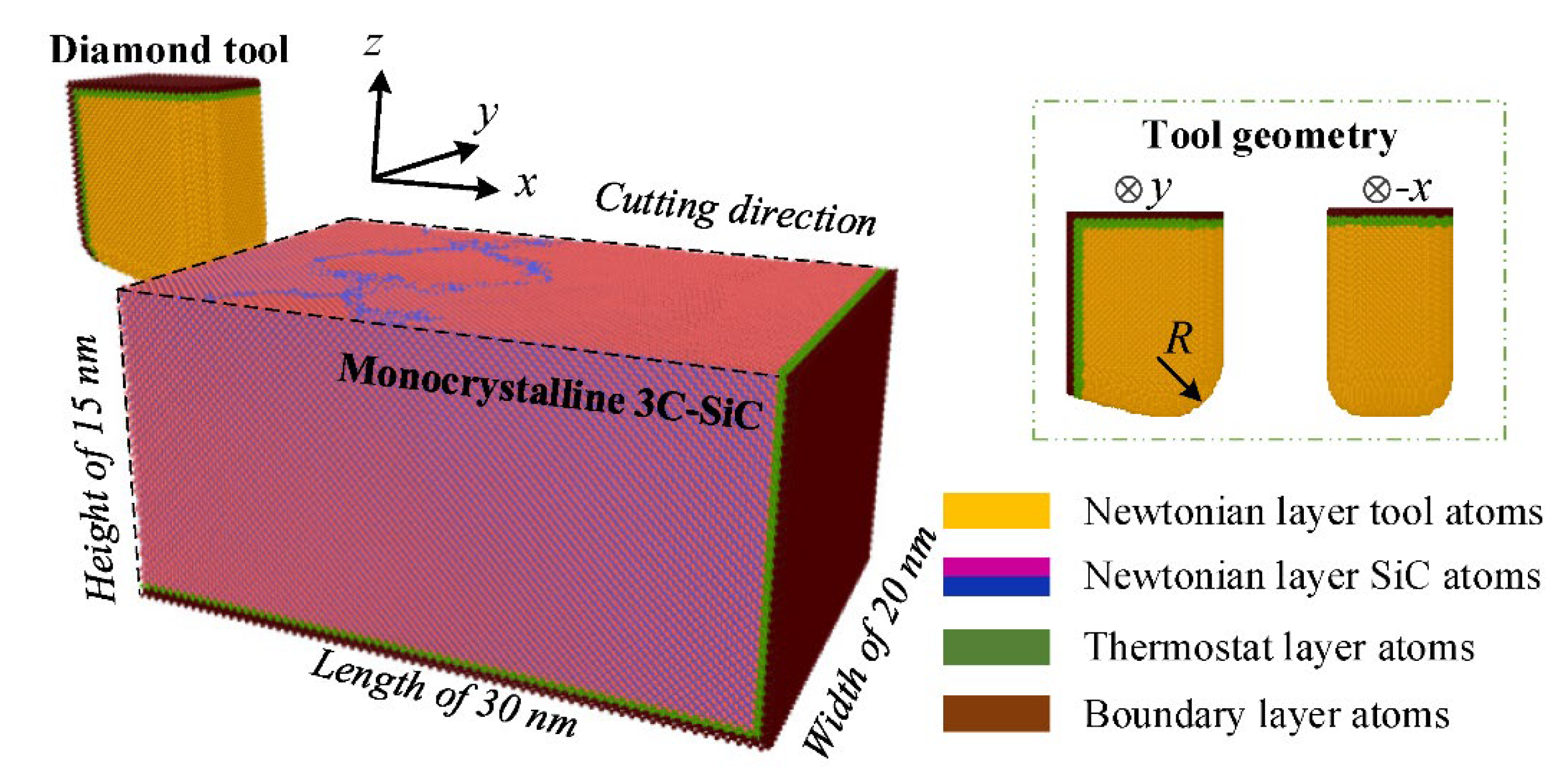
  201. Liu, B.; Li, X.; Kong, R.; Yang, H.; Jiang, L. A Numerical Analysis of Ductile Deformation during Nanocutting of Silicon Carbide via Molecular Dynamics Simulation. Materials 2022, 15, 2325. [Google Scholar] [CrossRef]
  202. Liu, J.; Dong, L.; Li, J.; Dong, K.; Wang, T.; Zhao, Z. Numerical Analysis of Multi-Angle Precision Microcutting of a Single-Crystal Copper Surface Based on Molecular Dynamics. Micromachines 2022, 13, 263. [Google Scholar] [CrossRef] [PubMed]
  203. Li, J.; Meng, W.; Dong, K.; Zhang, X.; Zhao, W. Study of Effect of Impacting Direction on Abrasive Nanometric Cutting Process with Molecular Dynamics. Nanoscale Res. Lett. 2018, 13, 11. [Google Scholar] [CrossRef] [PubMed]
  204. Ibrahim, A.F. Modeling the Abrasive Flow Machining Process (AFM) on Aluminum Alloy. Iraqi J. Mech. Mater. Eng. 2014, 32, 629–642. [Google Scholar]
  205. Singh, P.; Singh, L.; Singh, S. Manufacturing and performance analysis of mechanically alloyed magnetic abrasives for magneto abrasive flow finishing. J. Manuf. Process. 2019, 50, 161–169. [Google Scholar] [CrossRef]
  206. Geng, Y.; Fu, J.; Sarkis, J.; Xue, B. Towards a national circular economy indicator system in China: An evaluation and critical analysis. J. Clean. Prod. 2012, 23, 216–224. [Google Scholar] [CrossRef]
  207. Hong, L.; Li, H.; Gao, N.; Fu, J.; Peng, K. Random and multi-super-ellipsoidal variables hybrid reliability analysis based on a novel active learning Kriging model. Comput. Methods Appl. Mech. Eng. 2020, 373, 113555. [Google Scholar] [CrossRef]
  208. Shimizu, N.; Kaneko, H. Direct inverse analysis based on Gaussian mixture regression for multiple objective variables in material design. Mater. Des. 2020, 196, 109168. [Google Scholar] [CrossRef]
  209. Devriendt, S.; Antonio, K.; Reynkens, T.; Verbelen, R. Sparse regression with Multi-type Regularized Feature modeling. Insur. Math. Econ. 2021, 96, 248–261. [Google Scholar] [CrossRef]
  210. Srinivasan, R.; Jacob, V.; Muniappan, A.; Madhu, S.; Sreenevasulu, M. Modeling of surface roughness in abrasive water jet machining of AZ91 magnesium alloy using Fuzzy logic and Regression analysis. Mater. Today Proc. 2020, 22, 1059–1064. [Google Scholar] [CrossRef]
  211. Sankar, M.R.; Mondal, S.; Ramkumar, J.; Jain, V.K. Experimental investigations and modeling of drill bit-guided abrasive flow finishing (DBG-AFF) process. Int. J. Adv. Manuf. Technol. 2009, 42, 678–688. [Google Scholar] [CrossRef]
  212. Lam, S.S.Y.; Smith, A.E. Process Monitoring of Abrasive flow Machining Using a Neural Network Predictive Model. In Proceedings of the 6th Industrial Engineering Research Conference Proceedings, Miami Beach, FL, USA, 17–18 May 1997; pp. 477–482. [Google Scholar]
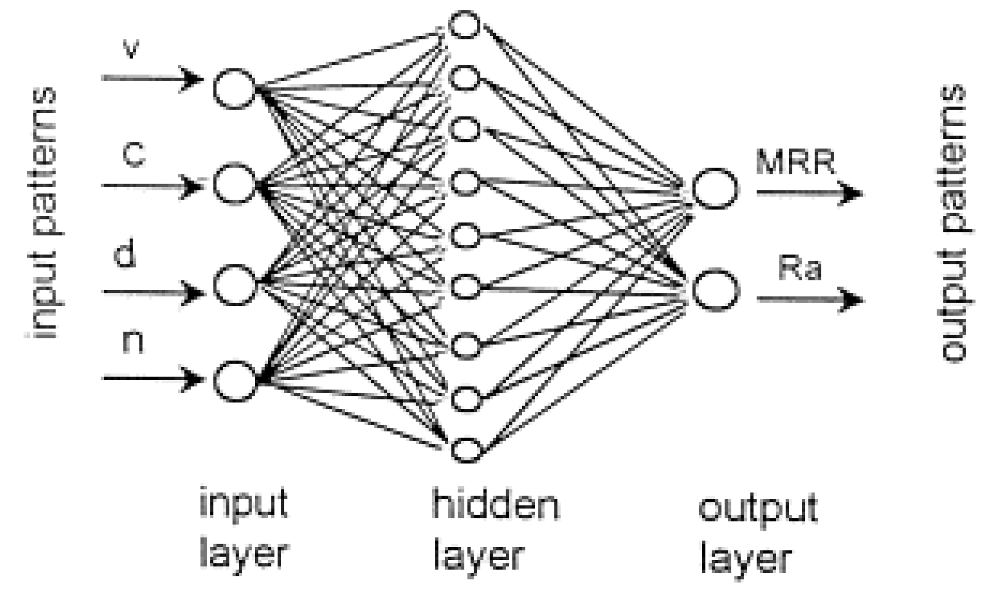
  213. Jain, R.; Jain, V.; Kalra, P. Modelling of abrasive flow machining process: A neural network approach. Wear 1999, 231, 242–248. [Google Scholar] [CrossRef]
  214. Rb, A.; Kr, S.K. Credit card fraud detection using artificial neural network. Int. J. Soft Comput. Eng. 2021, 2, 35–41. [Google Scholar] [CrossRef]
  215. Salgado, J.M.; Abrunhosa, L.; Venâncio, A.; Domínguez, J.M.; Belo, I. Combined bioremediation and enzyme production by Aspergillus sp. in olive mill and winery wastewaters. Int. Biodeterior. Biodegradation 2016, 110, 16–23. [Google Scholar] [CrossRef]
  216. Pandiyan, V.; Shevchik, S.; Wasmer, K.; Castagne, S.; Tjahjowidodo, T. Modelling and monitoring of abrasive finishing processes using artificial intelligence techniques: A review. J. Manuf. Process. 2020, 57, 114–135. [Google Scholar] [CrossRef]
  217. Jiang, H.; Xi, Z.; Rahman, A.A.; Zhang, X. Prediction of output power with artificial neural network using extended datasets for Stirling engines. Appl. Energy 2021, 271, 115123. [Google Scholar] [CrossRef]
  218. Mitrofanov, A.; Parsheva, K.; Nosenko, V. Simulation of an artificial neural network for predicting temperature and cutting force during grinding using CAMQL. Mater. Today Proc. 2020, 38, 1508–1511. [Google Scholar] [CrossRef]
  219. Effendy, N.; Ab Aziz, S.H.; Kamari, H.M.; Zaid, M.H.M.; Budak, C.E.A.; Shabdin, M.K.; Khiri, M.Z.A.; Wahab, S.A.A. Artificial neural network prediction on ultrasonic performance of bismuth-tellurite glass compositions. J. Mater. Res. Technol. 2020, 9, 14082–14092. [Google Scholar] [CrossRef]
  220. Marzban, M.A.; Hemmati, S.J. Modeling of abrasive flow rotary machining process by artificial neural network. Int. J. Adv. Manuf. Technol. 2017, 89, 125–132. [Google Scholar] [CrossRef]
  221. Bai, H.; Liu, C.; Breaz, E.; Gao, F. Artificial neural network aided real-time simulation of electric traction system. Energy AI 2020, 1, 100010. [Google Scholar] [CrossRef]
  222. Bourhis, Y.; Bell, J.R.; Bosch, F.V.D.; Milne, A.E. Artificial neural networks for monitoring network optimisation—a practical example using a national insect survey. Environ. Model. Softw. 2020, 135, 104925. [Google Scholar] [CrossRef]
  223. Gomes, D.M.; Smotherman, C.; Birch, A.; DuPree, L.; Della Vecchia, B.J.; Kraemer, D.F.; Jankowski, C.A. Comparison of Acute Kidney Injury During Treatment with Vancomycin in Combination with Piperacillin-Tazobactam or Cefepime. Pharmacother. J. Hum. Pharmacol. Drug Ther. 2014, 34, 662–669. [Google Scholar] [CrossRef]
  224. Zhou, L. Analysis of influencing factors of the production performance of an enhanced geothermal system (EGS) with numerical simulation and artificial neural network (ANN). Energy Build 2019, 200, 31–46. [Google Scholar] [CrossRef]
  225. Safa, B.; Arkebauer, T.J.; Zhu, Q.; Suyker, A.; Irmak, S. Latent heat and sensible heat flux simulation in maize using artificial neural networks. Comput. Electron. Agric. 2018, 154, 155–164. [Google Scholar] [CrossRef]
  226. Smith, A.E.; Slaughter, W.S. Neural Network Modeling of Abrasive Flow Machining. NISTIR 1997, 6079, 151–158. [Google Scholar]
  227. Selvan, M.C.P.; Midhunchakkaravarthy, D.; Senanayake, R.; Pillai, S.R.; Madara, S.R. A mathematical modelling of Abrasive Waterjet Machining on Ti-6Al-4V using Artificial Neural Network. Mater. Today Proc. 2019, 28, 538–544. [Google Scholar] [CrossRef]
  228. Selvan, C.P.; Midhunchakkaravarthy, D.; Pillai, S.R.; Madara, S.R. Investigation on abrasive waterjet machining conditions of mild steel using artificial neural network. Mater. Today Proc. 2019, 19, 233–239. [Google Scholar] [CrossRef]
  229. Deshpande, Y.V.; Zanwar, D.R.; Andhare, A.B.; Barve, P.S. Application of ANN modelling for optimisation of surface quality and kerf taper angle in abrasive water jet machining of AISI 1018 steel. Adv. Mater. Process. Technol. 2022, 13, 1–14. [Google Scholar] [CrossRef]
  230. Saini, S.K. Response parameters modeling of abrasive jet machined composite using artificial neural network. Mater. Today Proc. 2022, 62, 3860–3864. [Google Scholar] [CrossRef]
  231. Pérez-Salinas, C.F.; del Olmo, A.; de Lacalle, L.N.L. Estimation of Drag Finishing Abrasive Effect for Cutting Edge Preparation in Broaching Tool. Materials 2022, 15, 5135. [Google Scholar] [CrossRef]
  232. González, H.; Calleja, A.; Pereira, O.; Ortega, N.; de Lacalle, L.N.L.; Barton, M. Super Abrasive Machining of Integral Rotary Components Using Grinding Flank Tools. Metals 2018, 8, 24. [Google Scholar] [CrossRef]
  233. González, H.; Pereira, O.; Fernández-Valdivielso, A.; López de Lacalle, L.N.; Calleja, A. Comparison of flank super abrasive machining vs. flank milling on inconel® 718 surfaces. Materials 2018, 11, 1638. [Google Scholar] [CrossRef] [PubMed]
  234. Jain, R.K.; Jain, V.K. Optimum selection of machining conditions in abrasive flow machining using neural network. J. Mater. Process. Technol. 2000, 108, 62–67. [Google Scholar] [CrossRef]
  235. Ibrahim, A.M.; Hendawy, H.A.; Hassan, W.S.; Shalaby, A. Response surface and tolerance analysis approach for optimizing HPLC method. Microchem. J. 2019, 146, 220–226. [Google Scholar] [CrossRef]
  236. Wu, H.; Niu, W.; Wang, S.; Yan, S.; Liu, T. Sensitivity analysis of input errors to motion deviations of underwater glider based on optimized response surface methodology. Ocean Eng. 2020, 209, 107400. [Google Scholar] [CrossRef]
  237. Şenaras, A.E. Parameter Optimization Using the Surface Response Technique in Automated Guided Vehicles; Academic Press: Cambridge, MA, USA, 2019; pp. 187–197. [Google Scholar] [CrossRef]
  238. Hacıefendioğlu, K.; Başağa, H.B.; Banerjee, S. Probabilistic analysis of historic masonry bridges to random ground motion by Monte Carlo Simulation using Response Surface Method. Constr. Build. Mater. 2017, 134, 199–209. [Google Scholar] [CrossRef]
  239. Gao, W.; Chen, X.; Hu, C.; Zhou, C.; Cui, S. New damage evolution model of rock material. Appl. Math. Model. 2020, 86, 207–224. [Google Scholar] [CrossRef]
  240. Zhou, Z.; Li, D.-Q.; Xiao, T.; Cao, Z.-J.; Du, W. Response surface guided adaptive slope reliability analysis in spatially varying soils. Comput. Geotech. 2021, 132, 103966. [Google Scholar] [CrossRef]
  241. Hemmati, A. Using rate based simulation, sensitivity analysis and response surface methodology for optimization of an industrial CO2 capture plant. J. Nat. Gas Sci. Eng. 2019, 62, 101–112. [Google Scholar] [CrossRef]
  242. Joel, C.; Jeyapoovan, T.; Kumar, P.P. Experimentation and optimization of cutting parameters of abrasive jet cutting on AA6082 through response surface methodology. Mater. Today Proc. 2020, 44, 3564–3570. [Google Scholar] [CrossRef]
  243. Yunus, M.; Alsoufi, M.S. Application of response surface methodology for the optimization of the control factors of abrasive flow machining of multiple holes in zinc and al/sicp. J. Eng. Sci. Technol. 2020, 1, 655–674. [Google Scholar]
  244. Williams, R.E.; Rajurkar, K.P. Metal removal and surface finish characteristics in abrasive flow machining. Mechanical 1989, 38, 93–106. [Google Scholar]
  245. Bouland, C.; Urlea, V.; Beaubier, K.; Samoilenko, M.; Brailovski, V. Abrasive flow machining of laser powder bed-fused parts: Numerical modeling and experimental validation. J. Mater. Process. Technol. 2019, 273, 116262. [Google Scholar] [CrossRef]
  246. Jain, R.K.; Jain, V.K.; Dixit, P. Modeling of material removal and surface roughness in abrasive flow machining process. Int. J. Mach. Tools Manuf. 1999, 39, 1903–1923. [Google Scholar] [CrossRef]
  247. Pal, P.; Jain, K.K. Computational simulation of abrasive flow machining for two dimensional models. Mater. Today Proc. 2018, 5, 12969–12983. [Google Scholar]
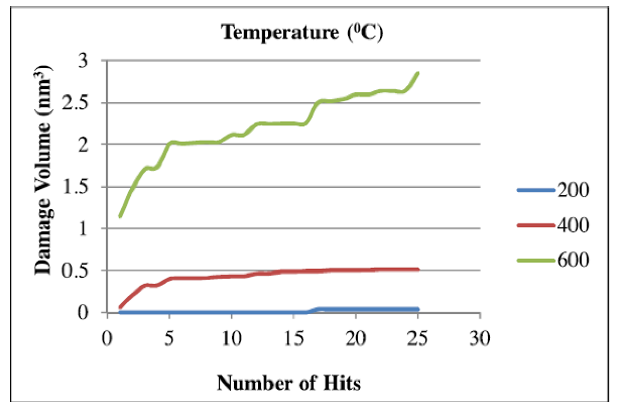
  248. Duong, N.; Kore, V.; Ma, J.; Lei, S.; Jahan, M.; Sundaram, M. Damage evolution in vibration assisted nano impact machining by loose abrasives at elevated temperatures: A numerical study. J. Manuf. Process. 2019, 47, 357–366. [Google Scholar] [CrossRef]
  249. James, S.; Sundaram, M. Effects of water molecules on material removal behavior in Vibration Assisted Nano Impact-machining by Loose Abrasives—A molecular dynamics simulation study. Procedia Manuf. 2018, 26, 552–559. [Google Scholar] [CrossRef]
  250. Wang, A.-C.; Tsai, L.; Liang, K.-Z.; Liu, C.-H.; Weng, S.-H. Uniform surface polished method of complex holes in abrasive flow machining. Trans. Nonferrous Met. Soc. China 2009, 19, s250–s257. [Google Scholar] [CrossRef]
  251. Kum, C.W. Modelling the abrasive flow machining process on advanced ceramic materials. J. Mater. Process. Technol. 2009, 20, 6062–6066. [Google Scholar]
  252. Sonia, P.; Kumari, S. Performance Evaluation Of Multi-Fibre (Hybrid) Polymer Composite. IOP Conf. Series: Mater. Sci. Eng. 2021, 1116, 012027. [Google Scholar] [CrossRef]
  253. Bandhu, D.; Vora, J.J.; Das, S.; Thakur, A.; Kumari, S.; Abhishek, K.; Sastry, M.N. Experimental study on application of gas metal arc welding based regulated metal deposition technique for low alloy steel. Mater. Manuf. Process. 2022, 1–19. [Google Scholar] [CrossRef]
  254. Kumari, S.; Nakum, B.; Bandhu, D.; Abhishek, K. Multi-Attribute Group Decision Making (MAGDM) Using Fuzzy Linguistic Modeling Integrated With the VIKOR Method for Car Purchasing Model. Int. J. Decis. Support Syst. Technol. 2022, 14, 1–20. [Google Scholar] [CrossRef]
  255. Tripathi, D.R.; Vachhani, K.H.; Bandhu, D.; Kumari, S.; Kumar, V.R.; Abhishek, K. Experimental investigation and optimization of abrasive waterjet machining parameters for GFRP composites using metaphor-less algorithms. Mater. Manuf. Process. 2021, 36, 803–813. [Google Scholar] [CrossRef]
  256. Wang, F.; Liu, S.; Ji, K. Numerical study on abrasive machining of rock using FDEM method. Simul. Model. Pr. Theory 2020, 104, 102145. [Google Scholar] [CrossRef]
  257. Chang, G.-W.; Yan, B.-H.; Hsu, R.-T. Study on cylindrical magnetic abrasive finishing using unbonded magnetic abrasives. Int. J. Mach. Tools Manuf. 2002, 42, 575–583. [Google Scholar] [CrossRef]
Figure 1. Loose abrasive-based machining process [26].
Metals 12 01328 g001
Figure 2. Categories of Loose Abrasive-Based Machining Process.
Metals 12 01328 g002
Figure 3. The machining accuracy of different traditional and advanced machining processes [27].
Metals 12 01328 g003
Figure 4. Surface roughness range comparison for traditional finishing processes.
Metals 12 01328 g004
Figure 5. Surface roughness range comparison for nano finishing processes.
Metals 12 01328 g005
Figure 6. AFM setups: (a) V-shape laboratory setup; (b) S-shape industrial setup [40].
Metals 12 01328 g006
Figure 7. Schematic of two-way AFM process.
Metals 12 01328 g007
Figure 8. Classification of AFM variants.
Metals 12 01328 g008
Figure 9. Defects in different areas: (a) metallization peels off of electronic components. (b) pipeline corrosion. (c) defective with gas pore. (d) defect big knot of textile materials. (e) shrinkage and porosity defect of Casting. (f) In the car body, defects in green, yellow, and orange bounding boxes are scratch, cratering, and hump. (g) Lack of defect of gear. (h) light leakage defect on mobile screen [25]. (i) Convexity defect in aluminum foil. (j) Scratch defect of the wheel hub. (k) Branch defect of wood veneer. (l) Bubble defect of the tire sidewall [87].
Metals 12 01328 g009
Figure 10. Modeling and simulation tools and techniques for “loose abrasive-based machining”.
Metals 12 01328 g010
Figure 11. Steps for applying the CFD in software.
Metals 12 01328 g011
Figure 12. Structural meshes: (a) Three-dimensional view of the computational domain and (b) axial profiles [129].
Metals 12 01328 g012
Figure 13. Abrasive particle velocity contour map: (a) NPR = 0.6, (b) NPR = 1, (c) NPR = 1.12 and (d) NPR = 2 [129].
Metals 12 01328 g013aMetals 12 01328 g013b
Figure 14. Volume fractions of abrasive particles: (a) NPR = 0.6, (b) NPR = 1, (c) NPR = 1.12 and (d) NPR = 2 [129].
Metals 12 01328 g014
Figure 15. (a) The 2D axisymmetric geometry model of a micro hole and (b) the mesh distribution [131].
Metals 12 01328 g015
Figure 16. Results of the flow simulation (a) pressure distribution, (b) shear rate distribution, (c) velocity distribution at the fixture region and as-machined region, as well as the (d) pressure curve, (e) shear rate curve, and (f) velocity curve at the wall of the as-machined region [131].
Metals 12 01328 g016
Figure 17. (a) The three-dimensional view of the media’s flow channels; (b) the mesh distribution, and (c) the 2D cross-section of micro porous structures, as well as the mesh metrics of (d) element quality and (e) skewness [132].
Metals 12 01328 g017
Figure 18. CFD simulation results of (a) pressure and (b) flow velocity in micro-porous holes [132].
Metals 12 01328 g018
Figure 19. CFD simulation results of (a) wall shear stress and (b) change rate of the flow velocity along z direction (axial direction) relative to x direction (radial direction) [132].
Metals 12 01328 g019
Figure 20. The geometry and boundaries of the computational domain and the numerical meshes: (a) Schematic diagram of the computational domain, (b) the mesh distribution and boundary settings for the AAJ simulation [133].
Metals 12 01328 g020
Figure 21. Evolution of particle jet flow along the jet flow direction in the AAJ micromachining. (a) The flow pattern inside the AAJ nozzle and (b) the particle distribution after the particles leave the nozzle exit [133].
Metals 12 01328 g021
Figure 22. The steps for the finite element method.
Metals 12 01328 g022
Figure 23. Flow chart of FEM-based Surface roughness and MRR calculation.
Metals 12 01328 g023
Figure 24. General process of coupling SPH with FEA [164].
Metals 12 01328 g024
Figure 25. (a) Process of determining the random number of abrasive particles; (b) SPH modeling of water and abrasive particles [164].
Metals 12 01328 g025
Figure 26. Hybrid FEM-BEM-DEM process for acoustic abrasive Polishing [165].
Metals 12 01328 g026
Figure 27. Workpiece position in the computational domain [165].
Metals 12 01328 g027
Figure 28. Vectors of particles’ velocity in different motion phases for the triangular wave at 70 Hz [165].
Metals 12 01328 g028
Figure 29. Discrete element method procedure.
Metals 12 01328 g029
Figure 30. Flow Chart of Simulation of DEM-based model.
Metals 12 01328 g030
Figure 31. The flowchart of the modeling framework of the MC method coupled with the DEM for multi-particle impact erosion [185].
Metals 12 01328 g031
Figure 32. Schematic illustrations of the stochastic abrasive particle flow in the computational model. (a) The generation procedure of multiple impacting particles is (b) the top view of particle footprints, where the dashed line represents the jet circle [185].
Metals 12 01328 g032
Figure 33. Model setup for the abrasive particle jet against the solid specimen in the DEM simulation [185].
Metals 12 01328 g033
Figure 34. The erosion process of micro-hole formation on glass by the overlapping impacts. (a) A snapshot of the material removal process, (b) the snapshots of the transient impact process under different impacting times [185].
Metals 12 01328 g034
Figure 35. The MDS procedure.
Metals 12 01328 g035
Figure 36. (a) Lattice optimization of the copper lattice with respect to cohesive energy, (b) dimensions of the atomistic model of p-Cu work material (a rectangular block of size 150 Å × 80 Å × 80 Å), and abrasive particle (spheres of sizes Ø43 Å and Ø57 Å) in perspective view, (c) front sectional view of the atomistic model of grains and their boundaries with initial height of abrasive and depth of nanoindentation and (d) equilibration graphs for cohesive energy and temperature for initial 25 ps [199].
Metals 12 01328 g036
Figure 37. (Nano-cutting process on p-Cu work material for cases (a,b) 1 and (c,d) 2 at Vlow. (a,c) atoms are colored in the z-direction to visualize the material removal during nano-cutting. (b,d) atomistic models of sectional views for start position, mid-position, and end position of abrasive during cutting at Vlow [199].
Metals 12 01328 g037
Figure 38. Molecular dynamics model of EVNC [200].
Metals 12 01328 g038
Figure 39. Comparative analysis of cutting force signals; ap = 6 Å, vw = 2 Å/ps, Az = 2 Å, f = 160 GHz (a) Tangential force signal (b) Normal force signal [200].
Metals 12 01328 g039
Figure 40. MD model of nanometric cutting on monocrystalline 3C-SiC [201].
Metals 12 01328 g040
Figure 41. The displacement vectors of the workpiece atoms during nanometric cutting at a distance of (a) 4 nm and (b) 16 nm [201].
Metals 12 01328 g041
Figure 42. Numerical analysis model of boron nitride particles cutting [202].
Metals 12 01328 g042
Figure 43. Cutting forces in different directions under various microcutting angles. (a) Cutting force in direction of [ 1 ¯ 00]. (b) Cutting force in direction of [0 1 ¯ 0]. (c) Cutting force in direction of [00 1 ¯ ] [202].
Metals 12 01328 g043
Figure 44. The structure of ANN [213].
Metals 12 01328 g044
Figure 45. (a) spherical abrasive grain removing schematic diagram. (b) the surface geometry [246].
Metals 12 01328 g045
Figure 46. Impact of volume fraction in strain rate [247].
Metals 12 01328 g046
Figure 47. Impact of volume fraction in horizontal velocity [247].
Metals 12 01328 g047
Figure 48. Impact of volume fraction in dynamic pressure [247].
Metals 12 01328 g048
Figure 49. The spherical diamond abrasive, the silicon workpiece, and the boundary conditions for the symmetric surface [248].
Metals 12 01328 g049
Figure 50. Effect of the number of hits in the variation of the damaged volume [250].
Metals 12 01328 g050
Figure 51. The principles of FDEM [256].
Metals 12 01328 g051
Figure 52. Cohesive elements failure process [256].
Metals 12 01328 g052
Figure 53. The magnetic forces that act in the X and Y directions on abrasive particles [257].
Metals 12 01328 g053
Figure 54. The parameters affect the MRF process.
Metals 12 01328 g054
Table 1. Literature summary of loose abrasive-based Machining process with basic principle and process parameters.
S. No.Loose Abrasive-Based MethodTypical MaterialsPrincipleAverage Surface Roughness (Ra µm)ApplicationRef.
1.Traditional Finishing ProcessesLappingMetalsHarden the trapped partials between the surface of the workpiece and a soft counter formal surface0.05 µm to 2.5 µmImproving the surface finish in loose abrasive-based machining[28]
Buffing and PolishingMetal and woodFinishing the surface is performed through a wheel or an abrasive0.1 µm to 0.41 µmSmoothing the material[29]
Super abrasive machiningTitanium, nickel-based alloys and metal matrix composites, etc.Finishing of Hard surfaces using polycrystalline diamond (PCD) or polycrystalline cubic boron nitride (PCBN) tools0.0127 µm–0.203 µmHard materials[28]
2Advanced finishing ProcessAbrasive Flow Machining (AFM)Hardened steelRemoving material from the surface of the material using sliding of abrasive particles of another material0.184 µmCan deal with complex components[26,28,30]
Elastic Emission Machining (EEM)siliconremoving the material atom by atom with no cracks, deformation, or deep indentationsLess than 0.0005 µmRemoving material in loose abrasive-based machining[28,30,31]
Chemical Mechanical Polishing (CMP)siliconA layer is formed between the workpiece and the slurry by chemical reaction. This layer is softer than the material of the original workpiece, which can be easily removed.0.005 µm to 0.01 µmused in the finishing of the wafers made from silicon[28,30,32]
Magnetic Abrasive Finishing (MAF)silicon nitrideIn this process, ferromagnetic particles are mixed with the particles of the workpiece. This mixture is brought close to the surface of the workpiece to be finished.Less than 0.01 µmFinishing the surface of nano-chips[28,30]
Magnetorheological Finishing (MRF)Flat BG7 glassTo finish the surface in this process, magnetorheological fluid (MR fluid) is used. This fluid consists of iron particles, carbonyl iron particles (CIPs), carrier fluid, and abrasive particles.
The viscosity of this fluid is increased when it comes under the effect of the magnetic field. The CIPS arrange along the magnetic force line, and then the abrasive particles are entangled within the chains, and their motion causes the material removal
Less than 0.001 µmFinishing micro/Nano-chips[28,30]
Magnetorheological Abrasive Flow Finishing (MRAFF) This method is an extended version of MRF. the extrusion of the medium of the magnetorheological polishing is performed through the surface of the workpieceLess than 0.001 µmFinishing softer material than MRF[30,33,34]
Ball end Magnetorheological Finishing (BEMRF)Metal mirror and glassfor the finishing, this process uses the rotating spot of the stiffened MR fluidLess than 0.001 µmUsed in the finishing of the complex 3d geometry[35]
Table 2. A summary of the differences and similarities of the different AFM process variants.
S. No.AFM VariantsWorking PrinciplesWorking Polishing Fluid (Media)Commercial Process Names
1.Ultrasonic-assistanceUse of ultrasonic vibration along the AFM fixtureViscoelastic polymer-based mediaUltrasonic float polishing (UFP)
Ultrasonic-assisted AFM (UAAFM)
2.Rotational-assistanceRotating the AFM fixtureViscoelastic polymer-based mediaRotational AFF (R-AFF)
Drill bit guided AFM (DBG-AFM) Helical AFM (HLX-AFM)
3.Magnetic-assistanceUse of permanent magnetMagnetic abrasive-based mediaMagnetic AFM (MAFM)
4.Magnetorheological assistanceUse of Electro-magnet and magnetorheological (MR) fluidMR fluid-based mediaMagnetorheological AFF
AFF (MRAFF)
Rotational-MRAFF (R-MRAFF)
4.Electro-chemical assistanceUse of Electrochemical machining process along with AFM processElectrolytes and Viscoelastic polymer-based mediaElectro-chemical assisted AFM(ECAFM)
Electro-chemical and Centrifugal force-assisted AFM (EC2A2FM)
5Centrifugal force assistanceUse of Centrifugal forcesViscoelastic polymer-based mediaCentrifugal force-assisted AFM (CFAAFM)
Thermal Additive centrifugal AFM (TACAFM)
Table 3. Literature summary of performance analysis of the AFM process regarding their process parameters.
S. No.Ref.Typical MaterialsApplicationSurface Roughness (µm)
1.Guo et al., 2020 [83]Inconel 718AM partsRa 0.1 μm was the final surface roughness value.
2.Mali et al., 2018 [84]ABSFDM printed partsChange in Ra 21.37 μm for the external surface and 6.27 μm for the internal surface was found.
3.Subramanian et al., 2016 [85]Co-Cr alloyBio-implant, i.e., Hip JointIt was found that the surface roughness decreased from beginning R, value 502 nm to final R, value 39 nm.
4.Kumar et al., 2015 [86]Ti-6Al-4VBio-implant, i.e., Knee JointThe final surface roughness was measured to be 35–78 nm.
Table 4. A summary of the differences and similarities of the different AFM process variants.
S. No.Ref.Workpiece MaterialApplicationsRemarks
1.Fu et al., 2016 [98]Nickel-based superalloyTurbine blades
  • Straight blade surface roughness in the AFM technique without guide blocks falls from 0.436 µm to 0.235 µm.
  • The blade surface roughness is reduced by the fixture with guide blocks from 0.513 µm to 0.141 µm.
2.Kumar and Hiremath, 2019 [99]SS 316 L, Ti-6Al-4VWettability biomaterials
  • AFM improves the wettability and surface quality of the implant while lowering the likelihood of bacterial adherence.
  • Even for the identical roughness values, wettability was reported to differ for the two work materials.
3.Petare et al., 2019 [100]20MnCr5Gear
  • Using AFM, the morphology of the gear tooth is improved. Using AFM, the gear tooth’s morphology is improved.
4.Singh and Sankar, 2020 [101]Surgical steelEDMed micro-slots
  • Surface roughness decreases from the initial value of Ra, 3.54 µm, to Ra, 0.21 µm.
4.Singh et al., 2020 [102]AluminumFinishing of cylindrical surfaces
  • With a final Ra of 0.22 µm, a surface finish improvement of 72.7% was seen throughout the process.
5Mohammadian et al. [103]Inconel 625SLM printed parts
  • Ra is decreased by 20% for a build orientation of 135° and by 45% for a build orientation of 15°.
Table 5. A summary of the shortcomings of simulation techniques for Abrasive-based machining processes.
S. No.Simulation TechniquesSoftware Package/Programming PlatformAdvantagesLimitations
1.Molecular Dynamic Simulation (MDS),GROMACS, CHARMM, AMBER, NAMD, and LAMMPS
  • To predict how disruption will affect a molecular system.
  • It predicted the simulation results at a molecular level.
  • Accuracy is very high
  • To find consistent differences in the outcomes, it is usually best to run numerous simulations of both the disturbed and undisturbed systems.
  • Computation time is very high.
  • Required high skilled computer programming.
  • Advanced and high configured computation platform is required.
2.Computational Fluid Dynamics (CFD),Ansys Fluent, COMSOL Multiphysics SolidWorks, and Autodesk Inventor CFD add-ons, OpenFOAM.
  • To study intricate fluid-fluid, fluid-solid, or fluid-gas interaction problems.
  • To observe the flow field in depth and in its entirety without any interference
  • User-friendly software platform is available.
  • High-accuracy results required a large number of iterations of a simulation run.
  • Computation time is high.
  • To perform the fast simulation, it needs high configured and advanced computation platform
3.Finite Element Method (FEM),Ansys Workbench, ANSYS APDL, Abaqus, etc.
  • Comprehensive result sets, providing the system’s physical response in any area, including ones that an analytical approach could have omitted.
  • Affordable and Faster Design Cycle.
  • The approach is approximate; rather than analyzing an actual structure, a model of it is used instead.
  • Accuracy is low. It depends on many factors like the quality of meshing.
4.Discrete Element Method (DEM),Altair EDEM
  • DEM can be used to simulate a wide variety of granular flow and rock mechanics situations.
  • DEM allows a more detailed study of the micro-dynamics of powder flows than is often possible using physical experiments.
  • DEM is only applicable to the micromechanics of the problem.
Table 6. Summary table of CFD-based modeling and simulation of the loose abrasive-based method.
ReferencesWork-Piece MaterialType of Abrasive-Based ProcessImportant Input and Output Variable ConsideredSoftware ToolRemarks
[94]hard materialsMagnetic field-assisted finishing (MFAF)Continuity and momentum-The active abrasive grain axial force is higher than the force of the reaction due to the strength of the material.
CFD is an effective tool for predicting the surface roughness in abrasive flow-based machining.
[93]Silicon carbideAbrasive flow machining (AFM)Shear modulus, elastic modulus, damping factor, stiffnessANSYS CFXCFD is an effective tool for predicting the surface roughness in abrasive flow-based machining.
[115]-Abrasive flow machining (AFM)“Density, the extrusion pressure, piston velocity, abrasive hardness, particle hardness and
media viscosity, workpiece hardness.”
ANSYS FLUENTThe process was a precision finishing operation. Therefore, the removed material is low. This amount can be increased with the increase in the number of cycles. The modeling and the simulation are very important due to the high number of parameters
[121]Visco-elastic materials“Ultrasonic assisted abrasive flow machining (UAAFM)”“Fluid pressure, the velocity profile of the fluid, temperature distribution in the working fluid, wall shear, angle of impact, and finishing rate”Commercial simulation tool for CFDThe impact angle ‘θ’ plays a major role in the machining process and improves effectiveness. Wall shear helps predict if the process has better finishing rates.
[134]Turbine bladesAbrasive wearSize and shape of quartz particles, leakage flow through clearance gaps, blade life, and efficiency. When compared with the data from the actual erosion in turbines, the CFD results give more information. The leakage flow through clearance gaps of guide vanes causes erosion in the runner blade inlet.
Table 7. Summary table of FEM-based modeling and simulation of the loose abrasive-based method.
ReferencesWork-Piece MaterialType of AbrasiveImportant Input and Output Variable ConsideredSoftware ToolRemarks
[166]-“Centrifugal force assisted abrasive flow machining” (CFAAFM)velocity, resultant pressure, and radial stressesANSYS.The finite element method has high efficiency in modeling and simulation the abrasive flow-based machining
[167]bearing steel (52,100)Abrasive flow machiningCutting speed, depth of the cutting, area of the cutting
[168]-“Ultrasonic Assisted Magnetic Abrasive Finishing (UAMAF)”.Material Removal Rate (MRR), finishing speed, the size and the concentration of abrasive material, surface roughness-The ability to calculate the volume of the job removed by an individual indented abrasive particle and the surface roughness is then evaluated.
[157]stainless steel (AISI-420)“Cylindrical Electro-Chemical Magnetic Abrasive Machining (C-EMAM)”Efficiency, Magnetic field distribution, surface roughness-FEM helps to know the magnetic field distribution in the location of the cylindrical job.
[158]-free abrasive polishing (CMP)pressure applied, speed of rotation, material removal rate, surface roughness, heat generation-An infrared camera is used along with FEM to study the process parameters.
[159]AerMet 100, IN738LC, BuRTiAbrasive Machining processSurface integrity, fluid delivery system, machine tool design-Grinding models were available and are compared and studied with the FEM results.
Table 8. Summary table of DEM-based modeling and simulation of the loose abrasive-based method.
ReferencesWork-Piece MaterialType of AbrasiveImportant Input and Output Variable ConsideredSoftware ToolRemarks
[155]Stainless steel and SicpolishingDensity, elastic modulus, Poisson ratio-The DEM is an efficient tool for modeling and simulating the abrasive flow machining
[186]Non-metallic materialsfixed abrasive machiningTool bond composition, diamond grain size, concentration, constant grain protrusionCutSPDC drill bits are studied
[181]Fused Silica GlassAbrasive grindingwet etch technique, SSD depth.-Subsurface Damage (SSD) is known as a significant method
Table 9. Summary table of MDS-based modeling and simulation of the loose abrasive-based method.
ReferencesWork-Piece MaterialType of AbrasiveImportant Input and Output Variable ConsideredSoftware ToolRemarks
[187]Silicon, aluminium,polishingWorkpiece materials, Abrasive particles, Boundaries, Group of atoms, Statistical Ensembles, TimestepTERSOFF and OVITOMDS is a very effective tool in modeling and simulating mechanical polishing.
The material removal from aluminium is higher than silicon.
[189]silicon carbide (SiC)Using diamond gritWorkpiece materials, boundary atom, scratching speed, Newtonian atomLAMMPS and OVITO
[203]crystal copperPolishing using SiC abrasive grainsAbrasive radius, the total of C atoms and Si atoms, numbers of carbon and silicon atoms, and the cutting angle-The small angle in the cutting process leads to higher accuracy
[194]GaNAbrasive machining“cutting velocity, depth of cut (DOC), abrasive shape, atomic strain, stress, temperature, cutting forces, and deformation layer”-MDS helps us to gain insights into the GaN behaviour when abrasive machining is performed
[195]diamondsChemical Mechanical Polishing (CMP)Pressure, precision, damage reductionReaxFFMolecular dynamics helps understand the theory to attain damage reduction and precision
Table 10. Summary table of MVRA-based modeling and simulation of the loose abrasive-based method.
ReferenceWork-Piece MaterialType of AbrasiveImportant Input and Output Variable ConsideredSoftware ToolRemarks
[210]Magnesium alloy (AZ 91)Abrasive Flow Machining (AFM)“Water pressure (WP), Traverse Speed (TS), Stand-off distance (SOD), and Surface Roughness” Regression equations were constructed using the input parameters, and the Surface roughness value is projected.
[126] Silicon   Nitride   ( S i 3 N 4 )Hot Abrasive Jet machining (HAJM)air pressure, nozzle tip-distance, and the temperature of the abrasive-The Regression models along with the Genetic Algorithm are used to predict the optimum process variables for HAJM.
[211]Aluminium alloysAbrasive flow machining (AFM)number of cycles, “percentage of abrasive concentration, extrusion pressure, and abrasive grain size, length of stroke”SPSSMVRA has high accuracy in modeling and simulation in Abrasive flow machining
Table 11. Summary table of ANN-based modeling and simulation of the loose abrasive-based method.
ReferenceWork-Piece MaterialType of AbrasiveImportant Input and Output Variable ConsideredSoftware ToolRemarks
[14]f Al/SiCp metal matrix composites (MMCs) components.“Abrasive flow machining (AFM)”Extrusion pressure, Abrasive mesh size,
Media viscosity grade
No. of finishing cycles
Percentage of abrasive concentration
-ANN has a small error and high efficiency in modeling and simulating LAM
[234]-“Abrasive flow machining (AFM)”Abrasive mesh size machining (AFM)-The results from the modeling and simulation using ANN match the experimental results.
[227]Ti-6Al-4VAbrasive Waterjet Machining (AWJM)--ANN aids in obtaining the optimum operative condition and control methods.
[228]Mild steelAbrasive waterjet machining (AWJM)depth of cut, surface roughness, water pressure, traverse speed, abrasive mass flow rate, and stand-off distance.MATLABFeeding the data to the ANN is followed by a back propagation algorithm to train the model.
Table 12. Summary table of RSA-based modeling and simulation of the loose abrasive-based method.
ReferenceWork-Piece MaterialType of AbrasiveImportant Input and Output Variable ConsideredSoftware ToolRemarks
[241]zinc and Al/SiCp composite materialsAbrasive flow machining (AFM)concentration, pump pressure, abrasive mesh size, number of cycles, and workpiece material.-RSA is an efficient tool used in abrasive flow machining in modeling and simulating metallic and non-homogeneous materials
[242]AA6082Abrasive Waterjet Machining (AWJM)surface roughness, material removal rate (MMR), hardness, abrasive feed, stand-off distance, and nozzle speed.-The main goal is to optimize the input parameters of the AWJM to get the least surface roughness with the highest MMR.
Table 13. Summary table of DDS-based modeling and simulation of the loose abrasive-based method.
ReferenceWork-Piece MaterialType of AbrasiveImportant Input and Output Variable ConsideredSoftware ToolRemarks
[107,243]metalAbrasive flow machining
(AFM)
number of cycles media viscosity, extrusion pressure-Media viscosity has a great effect on the performance of the process.
[106,244]-Abrasive flow machining
(AFM)
grain diameter, abrasive mesh size, mean grain diameter, the total volume of abrasive grains, the stroke length, the radius of media cylinder-Using stochastic simulation provides predicting the density of the active grain with high efficiency
Table 14. The validation of the CFD tool [247].
Boundary ConditionsApplied Parameters
Workpiece MaterialMild Steel
Modulus of elasticity of workpiece material202,086 MPa
Density of silicon carbide abrasive3220 kg/m3
Density of silly putty1140 kg/m3
Cylindrical workpiece dimensions
  • Diameter
  • Length
30 mm
47 mm
Diameter of medium cylinder87 mm
Average length of stroke34.5 mm
Abrasive grain size80 μm
Abrasive concentration60%
Publisher’s Note: MDPI stays neutral with regard to jurisdictional claims in published maps and institutional affiliations.

