
Experimental and Calphad Methods for Evaluating Residual Stresses and Solid-State Shrinkage after Solidification

Abstract
:1. Introduction
2. Materials and Methods
3. Results
4. Discussion
4.1. Experimental Method
4.2. Computational Method
4.3. Future Work
5. Conclusions
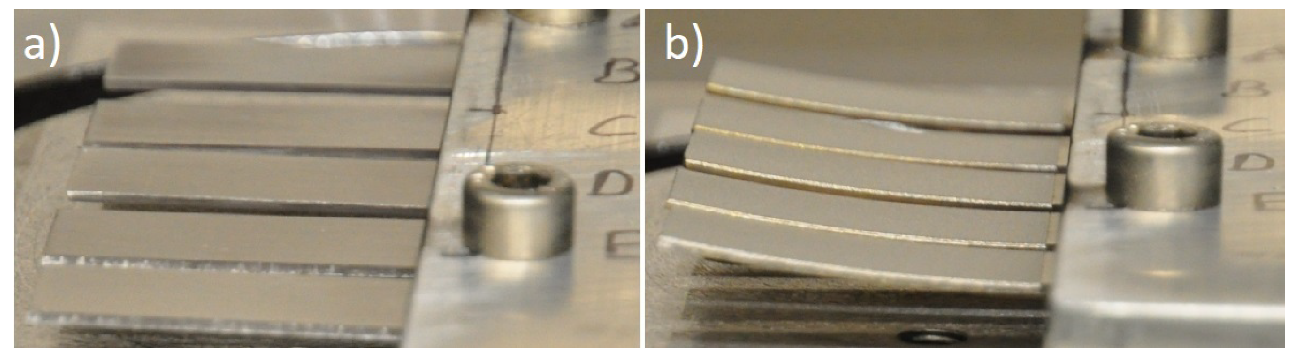
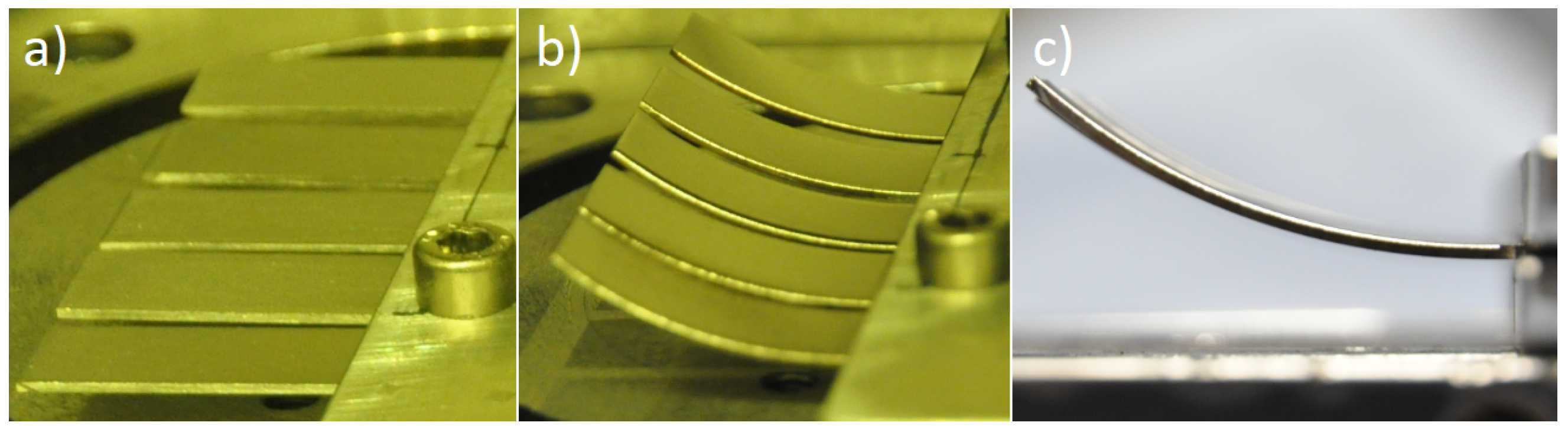
- No additive manufacturing required for residual stress analysis (Exp.)
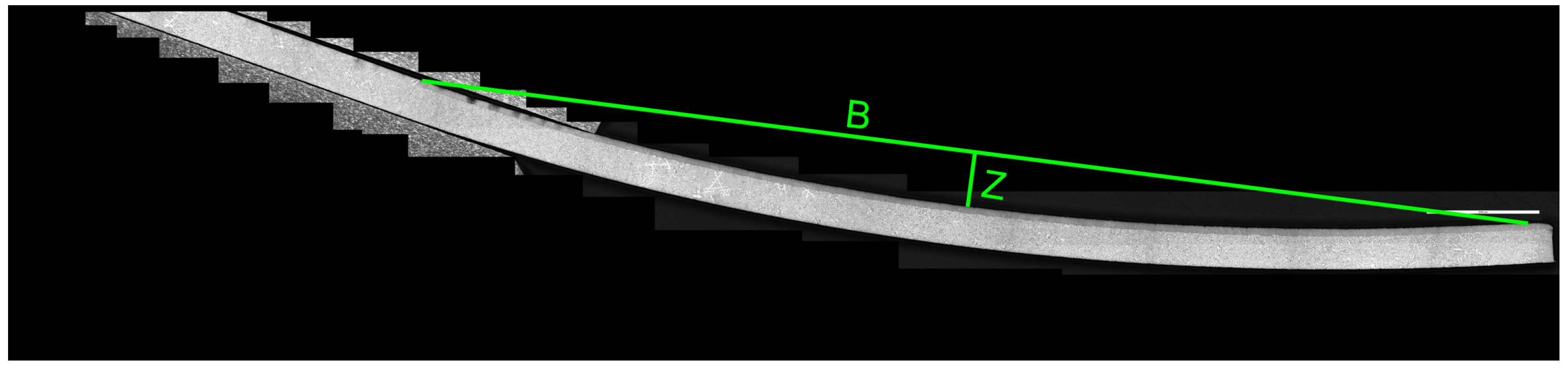
- Simple measurement from optical microscopy images (Exp.)
- Custom alloys can be tested without atomization (Exp.)
- Only chemical composition is required for calculating shrinkage (Comp.)
- Computationally inexpensive (Comp.)
- Trade-off between measurable curvature and plastic deformation (Exp.)
- Local plasticity in the heat affected zone difficult to mitigate (Exp.)
- Best for high yield strength alloys (Exp.)
- No plasticity taken into account (Exp. & Comp.)
- So far the simulations work best for single phased alloys (Comp.)
Author Contributions
Funding
Data Availability Statement
Acknowledgments
Conflicts of Interest
Abbreviations
| LPBF | Laser Powder Bed Fusion |
| AM | Additive Manufacturing |
| Finite Element Method | FEM |
| Direct energy deposition | DED |
| Linear coefficient of thermal expansion | CTE |
| Hexagonal close-packed | HCP |
| Body centered cubic | BCC |
| Face centered cubic | FCC |
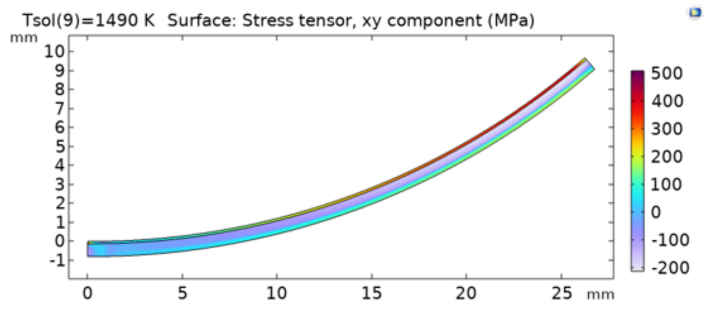
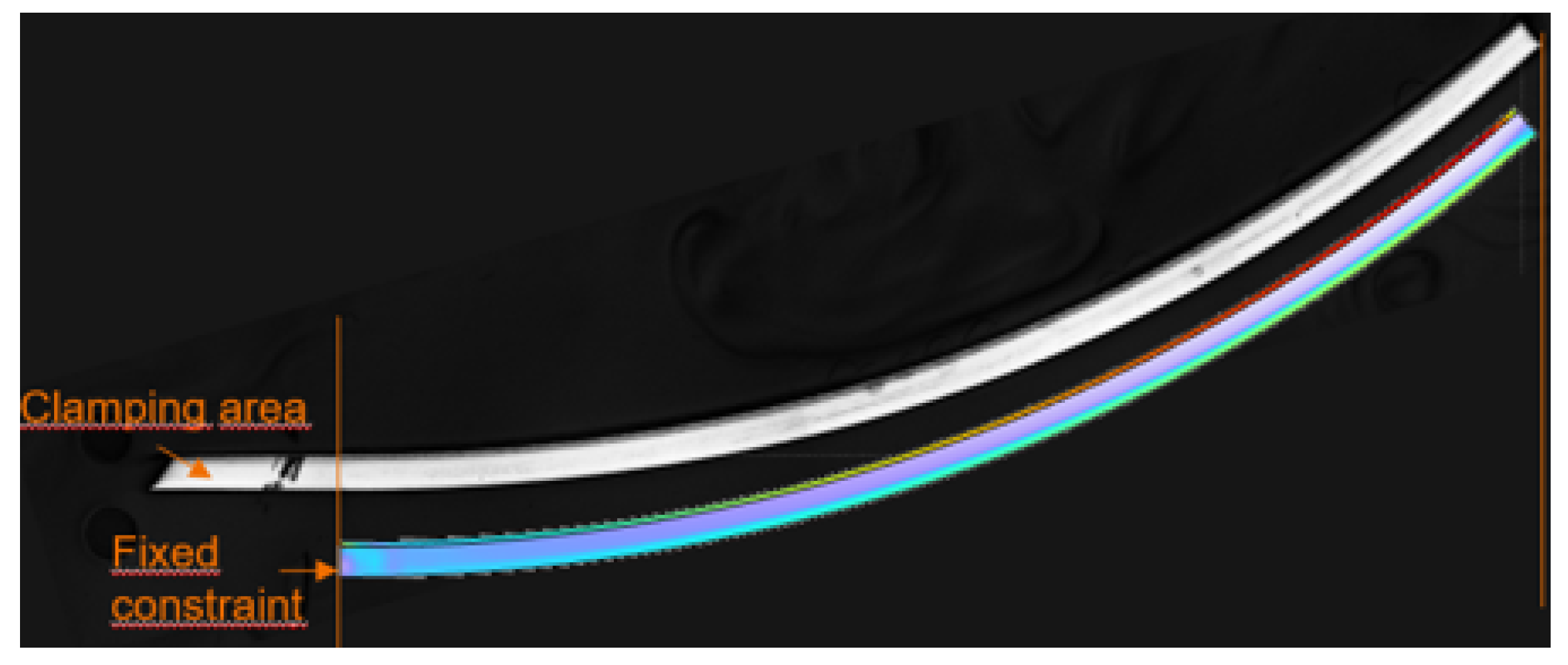
Appendix A. Plasticity Compensation of 316L with Comsol Multiphysics


| All Values in MPa | von Mises Stress | Stress Tensor, x Component | Stress Tensor, xy Component |
|---|---|---|---|
| Surface average Laser | 853.25 | 647.65 | 224.32 |
| Surface maximum Laser | 945.93 | 1065.8 | 508.26 |
| Surface average substrate | 281.94 | −117.2 | −40.924 |
| Surface maximum substrate | 559.67 | 463.63 | 185.26 |
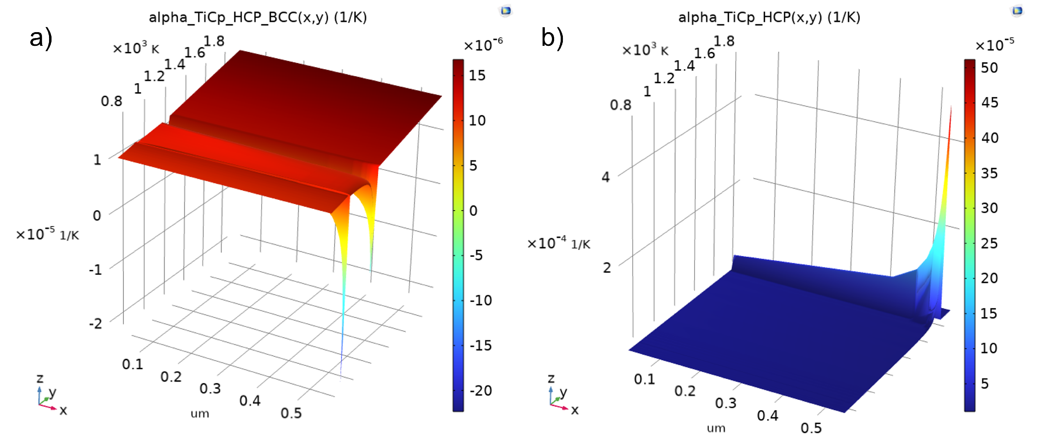
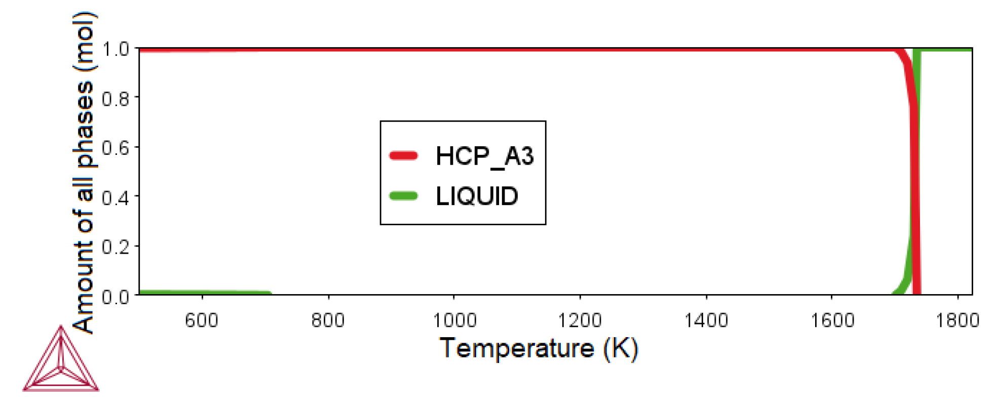
Appendix B. TiCp with HCP+Liquid

Appendix C. Dendrite Radius

References
- Herzog, D.; Seyda, V.; Wycisk, E.; Emmelmann, C. Additive manufacturing of metals. Acta Mater. 2016, 117, 371–392. [Google Scholar] [CrossRef]
- Salmi, A.; Atzeni, E.; Iuliano, L.; Galati, M. Experimental Analysis of Residual Stresses on AlSi10Mg Parts Produced by Means of Selective Laser Melting (SLM). Procedia CIRP 2017, 62, 458–463. [Google Scholar] [CrossRef]
- DebRoy, T.; Wei, H.; Zuback, J.; Mukherjee, T.; Elmer, J.; Milewski, J.; Beese, A.; Wilson-Heid, A.; De, A.; Zhang, W. Additive manufacturing of metallic components—Process, structure and properties. Prog. Mater. Sci. 2018, 92, 112–224. [Google Scholar] [CrossRef]
- Elsheikh, A.H.; Shanmugan, S.; Muthuramalingam, T.; Thakur, A.K.; Essa, F.A.; Ibrahim, A.M.M.; Mosleh, A.O. A comprehensive review on residual stresses in turning. Adv. Manuf. 2022, 10, 287–312. [Google Scholar] [CrossRef]
- Chen, S.-G.; Gao, H.-J.; Zhang, Y.-D.; Wu, Q.; Gao, Z.-H.; Zhou, X. Review on residual stresses in metal additive manufacturing: Formation mechanisms, parameter dependencies, prediction and control approaches. J. Mater. Res. Technol. 2022, 17, 2950–2974. [Google Scholar] [CrossRef]
- Pinomaa, T.; Yashchuk, I.; Lindroos, M.; Andersson, T.; Provatas, N.; Laukkanen, A. Process-Structure-Properties-Performance Modeling for Selective Laser Melting. Metals 2019, 9, 1138. [Google Scholar] [CrossRef] [Green Version]
- Keller, T.; Lindwall, G.; Ghosh, S.; Ma, L.; Lane, B.M.; Zhang, F.; Kattner, U.R.; Lass, E.A.; Heigel, J.C.; Idell, Y.; et al. Application of finite element, phase-field, and CALPHAD-based methods to additive manufacturing of Ni-based superalloys. Acta Mater. 2017, 139, 244–253. [Google Scholar] [CrossRef]
- Francois, M.; Sun, A.; King, W.; Henson, N.; Tourret, D.; Bronkhorst, C.; Carlson, N.; Newman, C.; Haut, T.; Bakosi, J.; et al. Modeling of additive manufacturing processes for metals: Challenges and opportunities. Curr. Opin. Solid State Mater. Sci. 2017, 21, 198–206. [Google Scholar] [CrossRef]
- Ahmed, S.H.; Mian, A. Influence of Material Property Variation on Computationally Calculated Melt Pool Temperature during Laser Melting Process. Metals 2019, 9, 456. [Google Scholar] [CrossRef] [Green Version]
- Fergani, O.; Berto, F.; Welo, T.; Liang, S.Y. Analytical modelling of residual stress in additive manufacturing. Fatigue Fract. Eng. Mater. Struct. 2017, 40, 971–978. [Google Scholar] [CrossRef]
- Chadwick, A.F.; Voorhees, P.W. The development of grain structure during additive manufacturing. Acta Mater. 2021, 211, 116862. [Google Scholar] [CrossRef]
- Zhang, C.; Yadav, V.; Moelans, N.; Juul Jensen, D.; Yu, T. The effect of voids on boundary migration during recrystallization in additive manufactured samples—A phase field study. Scr. Mater. 2022, 214, 114675. [Google Scholar] [CrossRef]
- Yang, M.; Wang, L.; Yan, W. Phase-field modeling of grain evolution in additive manufacturing with addition of reinforcing particles. Addit. Manuf. 2021, 47, 102286. [Google Scholar] [CrossRef]
- Lindroos, M.; Pinomaa, T.; Ammar, K.; Laukkanen, A.; Provatas, N.; Forest, S. Dislocation density in cellular rapid solidification using phase field modeling and crystal plasticity. Int. J. Plast. 2022, 148, 103139. [Google Scholar] [CrossRef]
- Lindroos, M.; Pinomaa, T.; Antikainen, A.; Lagerbom, J.; Reijonen, J.; Lindroos, T.; Andersson, T.; Laukkanen, A. Micromechanical modeling approach to single track deformation, phase transformation and residual stress evolution during selective laser melting using crystal plasticity. Addit. Manuf. 2021, 38, 101819. [Google Scholar] [CrossRef]
- Pinomaa, T.; Lindroos, M.; Walbrühl, M.; Provatas, N.; Laukkanen, A. The significance of spatial length scales and solute segregation in strengthening rapid solidification microstructures of 316L stainless steel. Acta Mater. 2020, 184, 1–16. [Google Scholar] [CrossRef]
- Lukas, H.; Fries, S.G.; Sundman, B. Computational Thermodynamics: The Calphad Method; Cambridge University Press: Cambridge, UK, 2007. [Google Scholar] [CrossRef]
- Gerstgrasser, M.; Cloots, M.; Stirnimann, J.; Wegener, K. Residual stress reduction of LPBF-processed CM247LC samples via multi laser beam strategies. Int. J. Adv. Manuf. Technol. 2021, 117, 2093–2103. [Google Scholar] [CrossRef]
- Soffel, F.; Eisenbarth, D.; Wegener, K. Effect of clad height, substrate thickness and scanning pattern on cantilever distortion in direct metal deposition. Int. J. Adv. Manuf. Technol. 2021, 117, 2083–2091. [Google Scholar] [CrossRef]
- Buchbinder, D.; Meiners, W.; Pirch, N.; Wissenbach, K.; Schrage, J. Investigation on reducing distortion by preheating during manufacture of aluminum components using selective laser melting. J. Laser Appl. 2014, 26, 012004. [Google Scholar] [CrossRef]
- Wang, D.; Wu, S.; Yang, Y.; Dou, W.; Deng, S.; Wang, Z.; Li, S. The Effect of a Scanning Strategy on the Residual Stress of 316L Steel Parts Fabricated by Selective Laser Melting (SLM). Materials 2018, 11, 1821. [Google Scholar] [CrossRef] [Green Version]
- Wu, A.S.; Brown, D.W.; Kumar, M.; Gallegos, G.; King, W.E. An Experimental Investigation into Additive Manufacturing Induced Residual Stresses in 316L Stainless Steel. Metall. Mater. Trans. 2014, 45, 6260–6270. [Google Scholar] [CrossRef]
- Prabhakar, P.; Sames, W.; Dehoff, R.; Babu, S. Computational modeling of residual stress formation during the electron beam melting process for Inconel 718. Addit. Manuf. 2015, 7, 83–91. [Google Scholar] [CrossRef] [Green Version]
- Denlinger, E.R.; Heigel, J.C.; Michaleris, P.; Palmer, T. Effect of inter-layer dwell time on distortion and residual stress in additive manufacturing of titanium and nickel alloys. J. Mater. Process. Technol. 2015, 215, 123–131. [Google Scholar] [CrossRef]
- Mertens, R.; Vrancken, B.; Holmstock, N.; Kinds, Y.; Kruth, J.P.; Van Humbeeck, J. Influence of Powder Bed Preheating on Microstructure and Mechanical Properties of H13 Tool Steel SLM Parts. Phys. Procedia 2016, 83, 882–890. [Google Scholar] [CrossRef] [Green Version]
- Macherauch, E. Introduction to Residual Stress. In Residual Stresses; Niku-Lari, A., Ed.; Pergamon Press: Cambridge, UK, 1987; pp. 1–36. [Google Scholar] [CrossRef]
- Bartlett, J.L.; Li, X. An overview of residual stresses in metal powder bed fusion. Addit. Manuf. 2019, 27, 131–149. [Google Scholar] [CrossRef]
- Stoney, G. The Tension of Metallic Films Deposited by Electrolysis. Proc. R. Soc. Math. Phys. Eng. Sci. 1909, 82, 172–175. [Google Scholar] [CrossRef] [Green Version]
- Brenner, A.; Senderoff, S. Calculation of stress in electrodeposits from the curvature of a plated strip. J. Res. Natl. Bur. Stand. 1949, 42, 105. [Google Scholar] [CrossRef]
- Ohring, M. Materials Science of Thin Films; Elsevier Science Technology: London, UK, 2001. [Google Scholar]
- Suhonen, T.; Varis, T.; Dosta, S.; Torrell, M.; Guilemany, J. Residual stress development in cold sprayed Al, Cu and Ti coatings. Acta Mater. 2013, 61, 6329–6337. [Google Scholar] [CrossRef]
- Simson, T.; Emmel, A.; Dwars, A.; Böhm, J. Residual stress measurements on AISI 316L samples manufactured by selective laser melting. Addit. Manuf. 2017, 17, 183–189. [Google Scholar] [CrossRef]
- Qiu, C.; Kindi, M.A.; Aladawi, A.S.; Hatmi, I.A. A comprehensive study on microstructure and tensile behaviour of a selectively laser melted stainless steel. Sci. Rep. 2018, 8, 7785. [Google Scholar] [CrossRef] [Green Version]
- Saarimäki, J.; Lundberg, M.; Moverare, J.; Brodin, H. 3D Residual Stresses in Selective Laser Melted Hastelloy X. Mater. Res. Proc. 2017, 2, 73–78. [Google Scholar] [CrossRef] [Green Version]
- Reijonen, J.; Antikainen, A.; Lagerbom, J.; Lindroos, M.; Pinomaa, T.; Lindroos, T. Laser powder bed fusion of high carbon tool steels. In Proceedings of the World PM2022 Congress Proceedings, Lyon, France, 9–13 October 2022. [Google Scholar]
- Lu, X.G.; Selleby, M.; Sundman, B. Theoretical modeling of molar volume and thermal expansion. Acta Mater. 2005, 53, 2259–2272. [Google Scholar] [CrossRef] [Green Version]
- MatWeb LLC. AISI Type 316L Stainless Steel, Annealed Sheet. Available online: https://www.matweb.com/search/DataSheet.aspx?MatGUID=1336be6d0c594b55afb5ca8bf1f3e042 (accessed on 20 June 2022).
- Antikainen, A.; Reijonen, J.; Lagerbom, J.; Lindroos, T. (VTT Technical Research Centre of Finland, Tampere, Finland). Additive manufacturing and heat treatment of high carbon cold work tool steel D2. Unpublished work. 2022. [Google Scholar]
- MatWeb LLC. Titanium Ti-6Al-4V (Grade 5), Annealed. Available online: https://www.matweb.com/search/DataSheet.aspx?MatGUID=a0655d261898456b958e5f825ae85390 (accessed on 20 June 2022).
- Electro Optical Systems GmBH. EOS Titanium Ti64 M290 Material Datasheet; CR326 11-17.
- MatWeb LLC. Titanium Grade 2. Available online: https://www.matweb.com/search/DataSheet.aspx?MatGUID=24293fd5831941ec9fa01dce994973c7 (accessed on 20 June 2022).
- Electro Optical Systems GmBH. EOS Titanium TiCp Grade 2 for M290 Material Datasheet; CR284 v01, 30 May 2016.
- MatWeb LLC. Special Metals INCONEL® HX Nickel Superalloy (UNS N06002). Available online: https://www.matweb.com/search/DataSheet.aspx?MatGUID=1fa55846a31c42119e5abd12fde717b8 (accessed on 20 June 2022).
- Electro Optical Systems GmBH. EOS Nickel Alloy HX for M290 Material Datasheet; TMS/0.2015.
- Mercelis, P.; Kruth, J. Residual stresses in selective laser sintering and selective laser melting. Rapid Prototyp. J. 2006, 12, 254–265. [Google Scholar] [CrossRef]
- Yin, Y.; Zhang, J.; Gao, J.; Zhang, Z.; Han, Q.; Zan, Z. Laser powder bed fusion of Ni-based Hastelloy X superalloy: Microstructure, anisotropic mechanical properties and strengthening mechanisms. Mater. Sci. Eng. 2021, 827, 142076. [Google Scholar] [CrossRef]
- Casati, R.; Lemke, J.; Vedani, M. Microstructure and Fracture Behavior of 316L Austenitic Stainless Steel Produced by Selective Laser Melting. J. Mater. Sci. Technol. 2016, 32, 738–744. [Google Scholar] [CrossRef]
- Antikainen, A.; Reijonen, J.; Lagerbom, J.; Lindroos, M.; Pinomaa, T.; Lindroos, T. Single-Track Laser Scanning as a Method for Evaluating Printability: The Effect of Substrate Heat Treatment on Melt Pool Geometry and Cracking in Medium Carbon Tool Steel. J. Mater. Eng. Perform. 2022. [Google Scholar] [CrossRef]
- Lee, W.S.; Chen, T.H.; Lin, C.F.; Luo, W.Z. Dynamic Mechanical Response of Biomedical 316L Stainless Steel as Function of Strain Rate and Temperature. Bioinorg. Chem. Appl. 2011, 2011, 173782. [Google Scholar] [CrossRef]
- British Stainless Steel Association. Elevated Temperature Physical Properties of Stainless Steels. Available online: https://bssa.org.uk/bssa_articles/elevated-temperature-physical-properties-of-stainless-steels/ (accessed on 7 July 2022).


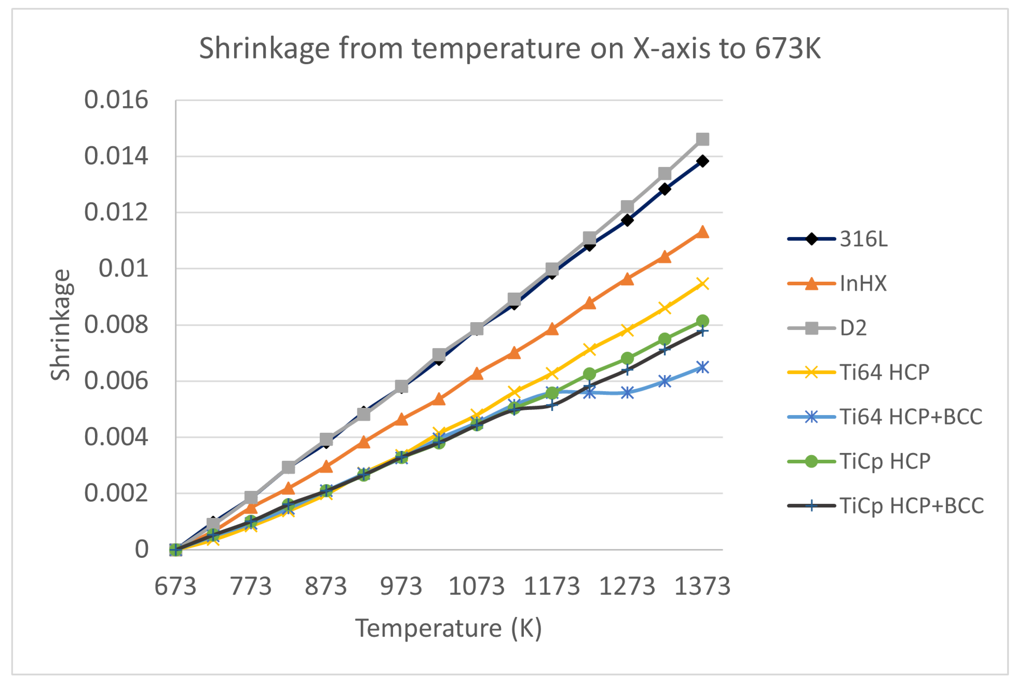
| Alloy | Scheil Solidus (K) | (1/K) -673 K | Linear Shrinkage -673 K |
|---|---|---|---|
| 316L | 1678 | 0.019 | |
| D2 | 1397 | 0.014 | |
| Ti64 | 1499 | 0.007 | |
| TiCp | 1919 | 0.015 | |
| In. HX | 1614 | 0.015 |
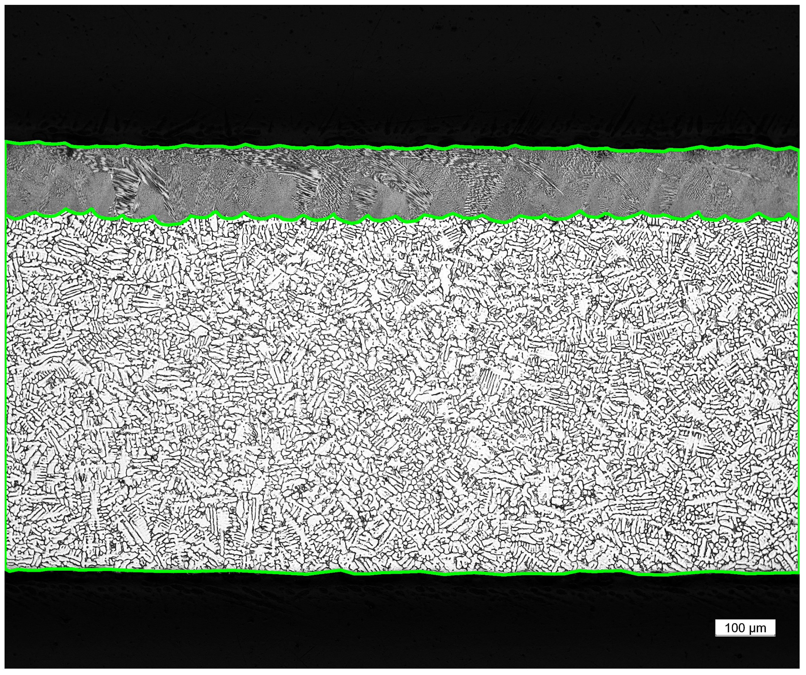
| Alloy | Melt (μm) | Base (μm) | Total (μm) |
|---|---|---|---|
| 316L | 131 ± 14 | 673 ± 5 | 803 ± 11 |
| D2 | 118 ± 1 | 592 ± 3 | 710 ± 3 |
| Ti64 | 184 ± 7 | 651 ± 11 | 835 ± 18 |
| TiCp | 193 ± 10 | 629 ± 13 | 822 ± 22 |
| Inconel Hx | 95 ± 3 | 840 ± 28 | 935 ± 28 |
| Alloy | Measured Res. Stress (MPa) | Base (MPa) | LPBF (MPa) | Young’s Modulus (GPa) |
|---|---|---|---|---|
| 316L | 3071 ± 214 | 170 [1] | 450 [1] | 193 [37] |
| D2 | 2134 ± 98 | >700 * | 1203 [38] | 190 [38] |
| Ti64 | 325 ± 18 | 880 [39] | 945 [40] | 114 [39] |
| TiCp | 372 ± 21 | 362 [41] | 560 [42] | 103 [41] |
| In. HX | 1709 ± 213 | 345 [43] | 630 [44] | 205 [43] |
Publisher’s Note: MDPI stays neutral with regard to jurisdictional claims in published maps and institutional affiliations. |
© 2022 by the authors. Licensee MDPI, Basel, Switzerland. This article is an open access article distributed under the terms and conditions of the Creative Commons Attribution (CC BY) license (https://creativecommons.org/licenses/by/4.0/).
Share and Cite
Antikainen, A.; Reijonen, J.; Lagerbom, J.; Lindroos, M.; Pinomaa, T.; Lindroos, T. Experimental and Calphad Methods for Evaluating Residual Stresses and Solid-State Shrinkage after Solidification. Metals 2022, 12, 1894. https://doi.org/10.3390/met12111894
Antikainen A, Reijonen J, Lagerbom J, Lindroos M, Pinomaa T, Lindroos T. Experimental and Calphad Methods for Evaluating Residual Stresses and Solid-State Shrinkage after Solidification. Metals. 2022; 12(11):1894. https://doi.org/10.3390/met12111894
Chicago/Turabian StyleAntikainen, Atte, Joni Reijonen, Juha Lagerbom, Matti Lindroos, Tatu Pinomaa, and Tomi Lindroos. 2022. "Experimental and Calphad Methods for Evaluating Residual Stresses and Solid-State Shrinkage after Solidification" Metals 12, no. 11: 1894. https://doi.org/10.3390/met12111894