

Using an Artificial Neural Network Approach to Predict Machining Time
by
 , , and
André Rodrigues
1,
Francisco J. G. Silva
1,2,*,
Vitor F. C. Sousa
1,2,
Arnaldo G. Pinto
1,
Luís P. Ferreira
1,2 and
Teresa Pereira
1,2 1
ISEP—School of Engineering, Polytechnic of Porto, Rua Dr. António Bernardino de Almeida 431, 4200-072 Porto, Portugal
2
INEGI—Institute of Science and Innovation in Mechanical and Industrial Engineering, Rua Dr. Roberto Frias 400, 4200-465 Porto, Portugal
*
Author to whom correspondence should be addressed.
Metals 2022, 12(10), 1709; https://doi.org/10.3390/met12101709
Submission received: 4 August 2022
/
Revised: 26 September 2022
/
Accepted: 7 October 2022
/
Published: 12 October 2022
(This article belongs to the Special Issue Machining: State-of-the-Art 2022)
Abstract
:One of the most critical factors in producing plastic injection molds is the cost estimation of machining services, which significantly affects the final mold price. These services’ costs are determined according to the machining time, which is usually a long and expensive operation. If it is considered that the injection mold parts are all different, it can be understood that the correct and quick estimation of machining times is of great importance for a company’s success. This article presents a proposal to apply artificial neural networks in machining time estimation for standard injection mold parts. For this purpose, a large set of parts was considered to shape the artificial intelligence model, and machining times were calculated to collect enough data for training the neural networks. The influences of the network architecture, input data, and the variables used in the network’s training were studied to find the neural network with greatest prediction accuracy. The application of neural networks in this work proved to be a quick and efficient way to predict cutting times with a percent error of 2.52% in the best case. The present work can strongly contribute to the research in this and similar sectors, as recent research does not usually focus on the direct prediction of machining times relating to overall production cost. This tool can be used in a quick and efficient manner to obtain information on the total machining cost of mold parts, with the possibility of being applied to other industry sectors.
1. Introduction
With a wide range of applications, plastics comprise a large and varied group of materials, essentially processed using heat and pressure. Injection molding is the leading plastic transformation process, and it is the most technical and the most widespread. It is used for mass production and has a high production rate of items, with tight tolerances and with little or no need for finishing operations [1]. The surface quality of the molded parts is incomparably superior to that of other competing technologies [2]. The injection-molding process requires an injection machine and a specially manufactured mold that defines the geometry of the final product. Despite having similar elements and structures, mold production is individual, which makes the mold-making industry project-driven. One of the primary sources of risk in managing these projects is the inaccurate prediction of manufacturing costs of the mold, which is usually produced using machining services and can influence, for example, up to 45% of a molded automotive part’s price [3].
Machining processes are some of the most relevant processes in the industry. The requirements of some parts, such as injection molds, are only fulfilled using these processes, which makes them irreplaceable [4,5]. Due to their complexity and popularity, many studies aim to understand and improve the different variables involved, not only in traditional but also in modern machining processes [6]. In recent years, part of the evolution of these processes is due, above all, to the progress registered in the performance of cutting tools, with the creation and implementation of coatings suited to different and challenging conditions [7,8]. Thereby, performance studies typically focus on the behavior of these coatings on difficult-to-machine materials [9,10]. All this research aims to identify the best cutting conditions for each situation, vibration being one of the main concerns among users [11]. The analysis of the cutting forces developed throughout the process can make a solid contribution to its stabilization and consequent efficiency [12]. Choosing the appropriate cutting parameters also safeguards the cutting operation and reduces process costs and energy consumption [13]. Some proposed models allow a 7.89% reduction in energy consumption [14] and seek to help operators balance energy consumption and processing costs at the same time [15]. Still, some surveys carried out by both manufacturers and end mill users reveal that the quality and process time is more relevant than energy savings [11], which is shown by some studies that prove that the decrease of processing time has more potential to increase energy efficiency than decreasing the process load [16]. The selection of the right machining strategy and cutting tool also plays a vital role in reducing cutting times, as well as the final cost and quality of the process [17]. Some authors seek to improve the calculation of some common cutting strategies, achieving a reduction in cutting forces and longer tool life [18] or reducing machining time by more than 55% [19]. Other approaches have shown that the sequence of cutting tools used can influence the amount of energy consumed and the cost of the process [20], and that the correct planning of operations allows for the reduction of errors, setup times, and non-productivity times [21]. The machining strategy used also influences the roughness and quality of the surface produced [22,23], as well as the wear of the cutting tools [24]. Trying to cool and lubricate the cutting contact area, the cutting fluids also optimize the performance of the cutting tools and, consequently, the entire process [25]. However, the use of conventional cutting fluids has proved to be a threat to the environment and the health of operators. Therefore, the use of solid lubricants has been the subject of several studies, proving to be an economic and ecological alternative in addition to offering better material removal rates and surface quality [26], as well as increased tool life [27]. Cryogenic cutting has also been analyzed, which leads to a reduction in tool wear, energy consumption, surface roughness, machining costs, and carbon emissions [28]. Both solid lubricants and cryogenic cutting have proved to be better alternatives to traditional machining processes. Often neglected, the part clamping system also plays a critical role in machining processes, guaranteeing easy operation to reduce setup time and the number of assemblies while ensuring the quality of the cutting process [4]. Some studies increased the number of parts machined per day by 32% [29] and reduced the machining time by applying suitable modular jigs [30].
All these variables make the machining process complex and difficult to budget, which is one of the main difficulties of machining services. It is common practice to set an hourly cost for the service and to determine the cost of manufacturing a part as a function of its machining time. Machining times, in turn, are commonly determined either through calculation or through human analysis. In the first case, CAM software simulates the operative sequences and the time needed to manufacture the part. In the second, the machining time is defined by a human evaluator based on a visual analysis of the part and their experience in this type of task. The first method is more accurate but requires more time to calculate machining time. The second one is faster but, as it depends on human analysis, it is less accurate, which can lead to underestimation of budgeting, resulting in losses for the company, or overestimation of budgeting, which will drive away potential customers. Thus, different studies have been developed to improve the cost estimation operation related to injection molds, with some methods showing high accuracy in applying cost drivers to estimate the cost of the manufacturing phases of the mold [31], while other authors proposed an analytic approach to determine the cutting time [32]. Other research focuses on calculating the machining cost according to cutting speed [33].
With a broad spectrum of applications in the industrial world, artificial neural networks (ANN) are mathematical models that, inspired by the functioning of the human brain, seek to understand complex relationships existing in each set of data. Therefore, some studies aim to assist in estimating manufacturing costs for different components [34,35] and to optimize the injection mold manufacturing process by implementing ANN [36,37]. The application of ANN in improving the performance of the machining process has also been studied [38,39], making it possible to predict machined surface roughness [40] and production quality [41], cutting tool wear [42], and cutting forces [43,44], as well as other computational approaches [45]. Regarding cutting tool condition monitoring, this is a very useful manner to evaluate the process’s overall stability and productivity [46], contributing to overall process improvement and a reduction in the production costs. There are various opportunities to implement ANN and other computational methods for machining tool monitoring [47], either for milling or for turning [48], contributing to an improvement of these processes, particularly regarding fewer tool exchanges and quality improvements of machined parts [49]. Some authors proposed artificial neural networks for feature recognition [50] to further establish relationships between the number of features and the cost of the part [51]. Other authors presented models using ANN to estimate machining time with average errors of 10.20 min [52] or to estimate injection mold manufacturing time with a percentage error of less than 25% [53]. Artificial intelligence tools to estimate manufacturing costs in the design phase have also been studied [54] as the effectiveness of different types of ANN in estimating machining times [55].
As seen from the studies presented in the previous paragraph, the use of ANNs can be quite useful in predicting the cost of manufacturing a certain part. However, there are some constraints regarding the use of this approach, with some approaches showing high degrees of error or deviation [53]. Despite this, there is potential for application of these ANNs in predicting these costs and thus in aiding budgeting operations for machining services. Thus, the budgeting process is time-consuming, prone to mistakes, and heavily dependent on previously acquired empirical knowledge. It is known that the machining time, especially for mold machining operations, is the most impactful parameter on the overall cost of the tool. Given this, by predicting the machining time, a somewhat accurate prediction of the final part’s cost can be made. In the present paper, a methodology for using an ANN to predict machining times for standard injection mold parts is presented by choosing and comparing different architectures, input data, and training variables, and thus finding the most accurate way of predicting machining times. The implementation of this ANN was compared to the previously employed method, in which the time is determined through careful modelling and simulation of the part. This is an expensive and time-consuming way of cost-estimating the machined parts. By employing the ANN presented in this work, companies should have a fast and accurate way of predicting the machining times of their produced parts.
2. Methods
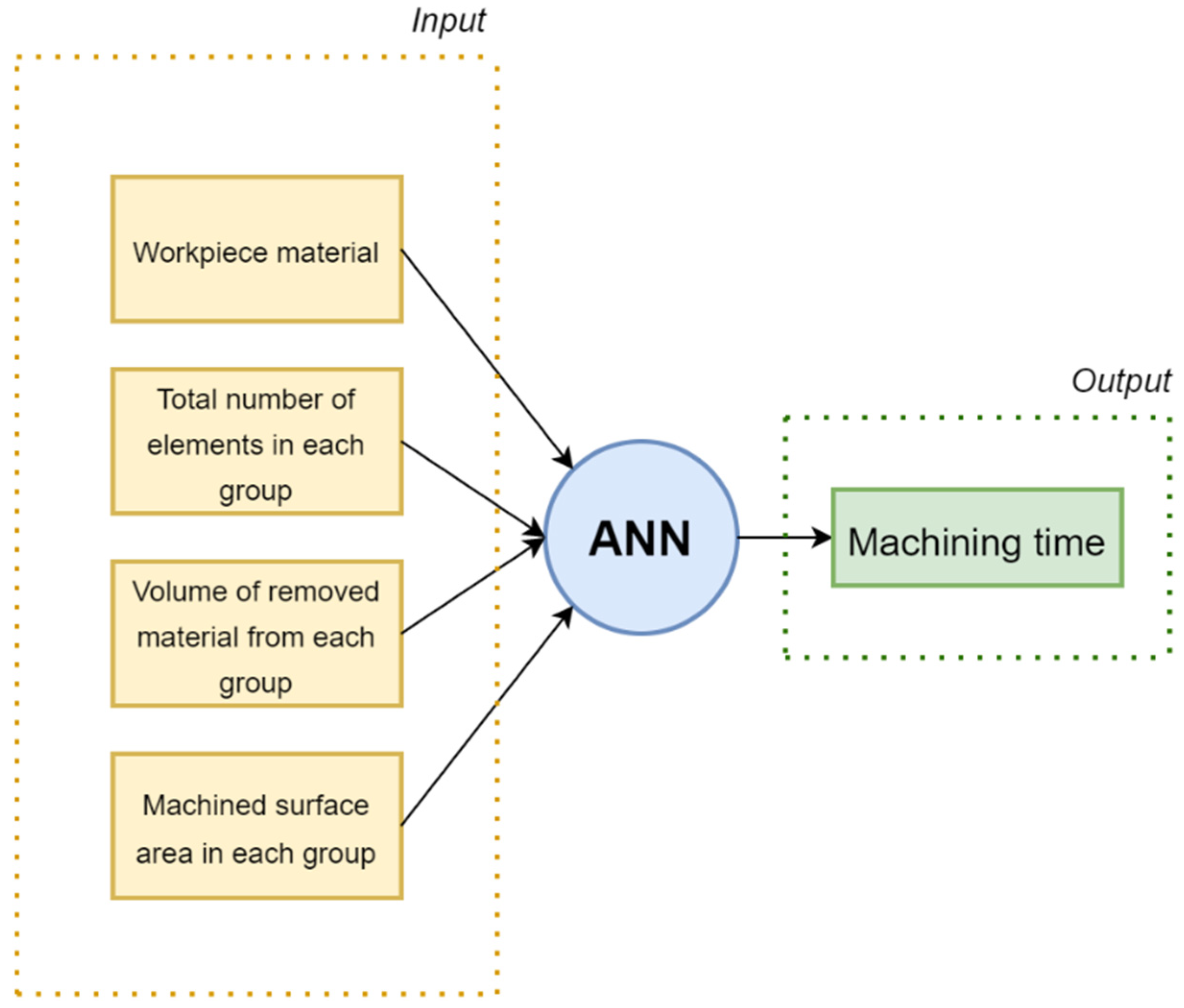
The present work aims at creating an artificial neural network (ANN) mode that allows the machining time of standard plastic injection mold parts to be estimated in a quick and effective way. For this purpose, it was considered that these parts usually present groups of similar features, which only diverge in dimensions, such as metric threads, clearance holes, fitting holes, rectangular and circular pockets, among others. Thus, the proposed solution consists of an ANN whose input variables are (see Figure 1):
- The workpiece material;
- Each feature group’s total number of elements;
- The volume of removed material from each feature group;
- The surface area machined in each feature group.
2.1. Data Preparation
Data preparation was the first step in the development of the ANN. The goal was to simulate a machining process, calculating the machining time of several plastic injection mold plates using CAM programming software (MasterCAM® 2022), and a library of tools created for this purpose. As seen before, the amount of data used for training the ANN influences its accuracy, making it necessary to calculate the machining time of hundreds of different parts to generate enough data. The traditional method for calculating machining times requires a 3D model and the CAM programming of each part, which is time-consuming considering the high number of parts needed; usually this calculated time is then compared to the actual required machining time to produce a said part. Therefore, an empirical-based method was created where the machining time of each element is calculated individually and subsequently assigned to each part at random, allowing the calculation of a multitude of different parts. The workpiece material and the machined geometries are defined based on common requests obtained to produce injection mold parts. These parts are usually standardized. Furthermore, literature research provided insight on the best-suited parameters and strategies to produce said parts. This information is complemented by contacting manufacturers of these standardized components. They usually offer practical and industrially acquired knowledge, which can be very useful when defining these parameters. Then, the machining times of 30 modeled parts are calculated by the traditional (simulation and modeling, offering a comparison of measurements made after component production) and empirical methods to compare the obtained values and validate the devised empirical method. A definition of these methods can be found below:
- Traditional method: To try and predict the required machining time to produce a certain part, these must be modelled in 3D. Subsequently, the CAM program is performed, and the machining time is estimated. Afterwards, these times are validated with those obtained from the part production itself. It is accurate; however, it is also time-consuming and cost inefficient;
- Empirical method: Input and output data are generated for the training of the ANNs, based on the machining time of individual operations (standardized machining operations for mold production). These operations are then compiled and considered for each of the produced part (Figure S1).
2.1.1. Features Definition and Sequence of Operations
The features used in this work are presented in Table 1, and the sequence of operations is also defined. This sequence of operations is defined based on the information displayed on the previous section (Section 2.2. Data preparation). In addition to the operations mentioned in Table 1, more machining operations were considered, such as circular and rectangular cavities, guiding holes, and low-depth circular cavities.
2.1.2. Machining Time Calculation
The workpiece material also significantly influences the final machining time by influencing the cutting parameters possible to use with the selected cutting tools. Therefore, two tool steels commonly used in injection mold structures were considered (Table 2).
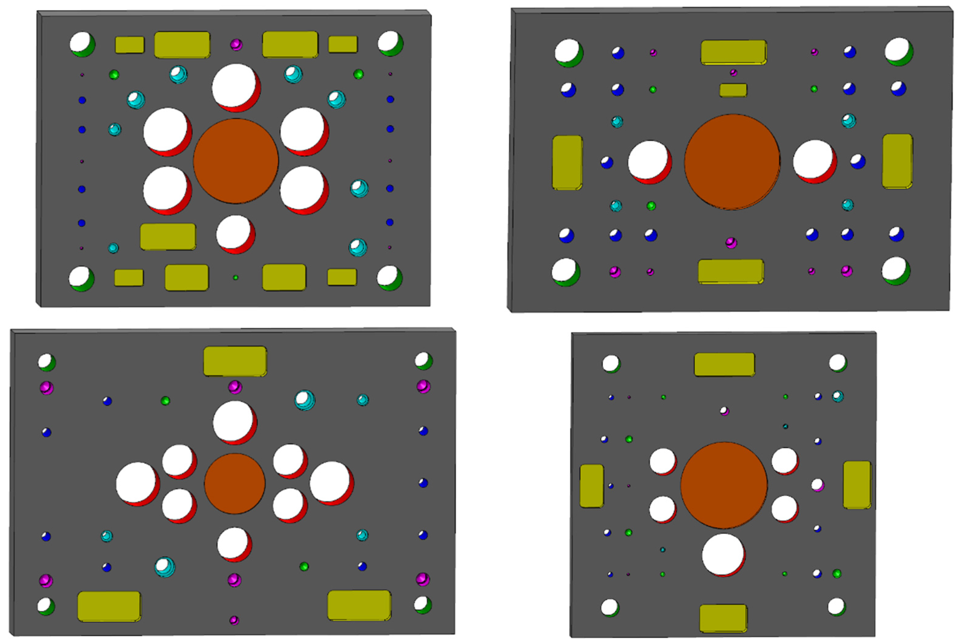
Based on the features presented in Table 1 and the materials to be machined in Table 2, 30 parts like the one shown in Figure 2 were generated and modeled. Each of the parts was assigned to one of the workpiece materials, as well as the elements in Table 1 in different quantities. Subsequently, and based on the sequences of operations assigned for each feature, a library of cutting tools was created, and machining strategies were defined.
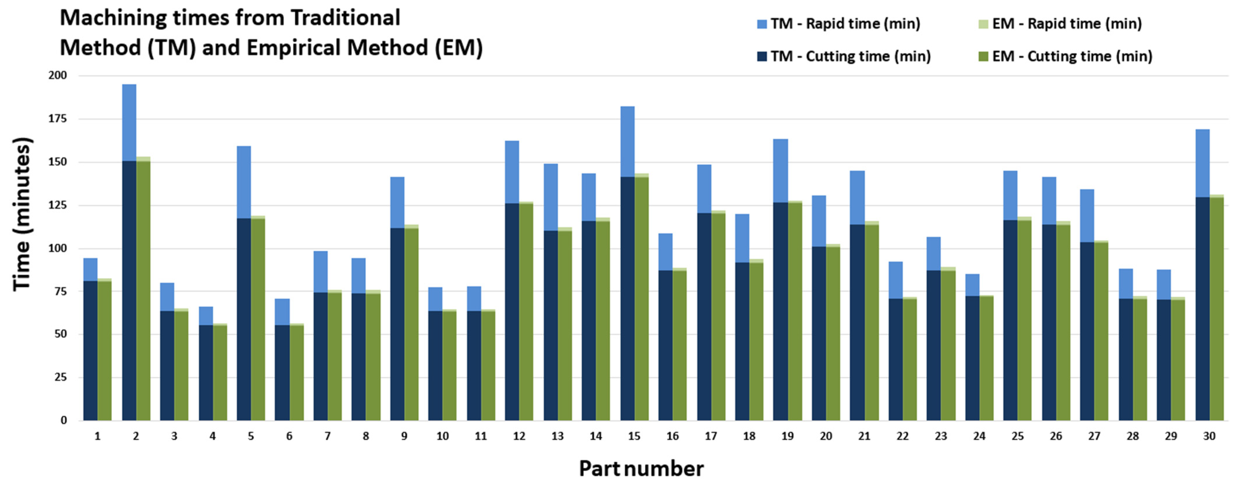
Then, the 30 parts were calculated using traditional and empirical methods, with the machining times obtained being shown and compared in Figure 3.
2.1.3. Validation of the Empirical Method
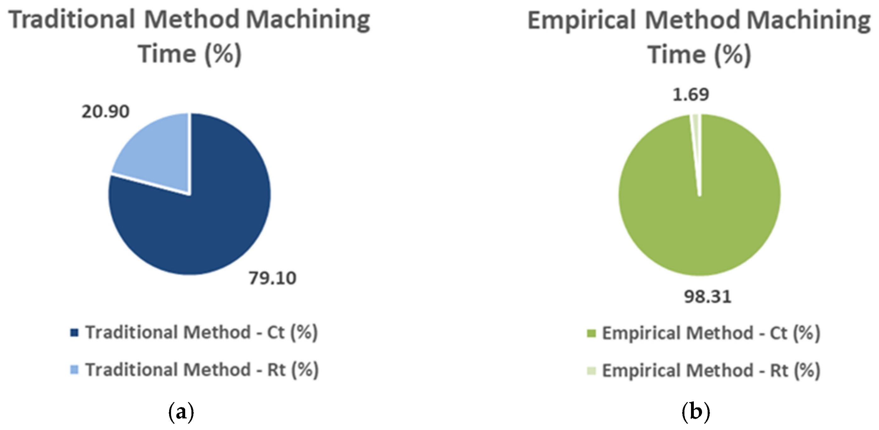
Machining times are divided into cutting time (Ct) and rapid travelling (Rt) movement time when the tool approaches the workpiece and moves between elements. These times are shown in Figure 3 and allow one to conclude that the cutting times obtained in the two methods are the same, which is explained by the fact that the same tools were used with the same cutting parameters and sequence of operations. The difference between the values obtained is in the rapid movement times. In the traditional method, the tool displacement time between elements and the tool approach time to the workpiece is calculated, while in the empirical method, due to lack of knowledge about the position of the elements in the workpiece, only the tool approach time is counted. This is the main reason for the difference in times obtained between these two methods. Thus, the empirical method is valid for calculating cutting times but is invalid for calculating rapid movement times. Thus, bearing in mind that they are the primary influence on the final machining time, as seen in Figure 4, only cutting times are used to develop the artificial neural networks.
After the validation of the empirical method, which has the advantage of being able to generate an infinite number of parts, two databases were created based on the features shown in Table 1 for the development of ANNs:
- trainingdata: database with 750 parts for training, testing, and validation of ANNs to develop;
- testdata: database with 100 parts to evaluate the performance of the developed ANNs.
2.2. ANN
The back error-propagation algorithm is one of the most used algorithms in engineering prediction models, being mainly used in layered feed forward ANNs. This algorithm is trained considering several series of examples (database), which encompass input arrangements and the desired output ranges. In this kind of algorithm, the input is introduced to the network, and the error between the current and the desired output is propagated backward in the network to calibrate the weights to improve the predictions accuracy. Several ANNs were developed to find the one that best fit the proposed problem. The ANNs were developed using MATLAB®, with the ‘feedforwardnet’ command, as it is suitable for regression problems where the objective is to estimate a specific numerical result with a single output, and with 80% of the data for training, 10% for validation, and the remaining 10% for testing. The activation function of the hidden layers was the ‘tansig’ function, and the last layer’s activation function, the ‘purelin’ function. ‘Tansig’ is a hyperbolic tangent sigmoid activation function generally used in intermediate layers of ANNs, since it is entirely derivable and compatible with most training algorithms used. ‘Purelin’, in turn, is a linear activation function used in regression problems. The algorithms used in the network training are the default ones for the ‘feedforwardnet’ command in MATLAB®.
Although ANNs are tested immediately after training, it was decided to test the developed ANNs in estimating the machining times of the 100 parts contained on the database ‘testdata’. In this way, the performance of the ANNs are evaluated against the same input data and not against random data. The evaluation of the network’s performance is conducted by calculating the mean error (ME), the mean absolute error (MAE), the mean squared error (MSE), and the percentage error (PE) between the real and estimated values. The maximum error (EMax) is also analyzed.
The mean error (ME) was calculated according to the expression:
where et is calculated as the difference between the real time (Zt) and the estimated time (), according to the expression:
The mean absolute error (MAE), in turn, is obtained according to:
Expression (4) was used to calculate the mean square error (MSE):
The percentage error was calculated according to the expression:
2.3. Comparative Methods
The first test looked at the network architecture with the best accuracy. The 750 parts of the ‘trainingdata’ database were used. The input variables of these networks were the quantity and volume of each of the features groups and the material of the workpiece. The second one sought to study the influence of the amount of input data on ANN accuracy. For this purpose, the ANN network architecture with the lowest percentage error of Test 1 was used, differing from the amount of data used in training. Test 3 studied the influence of input variables on the accuracy of ANNs. Once again, and keeping the percentage error as a criterion, the best ANN from the previous tests was selected, and the input variables were studied. Workpiece material was always used as input. To understand the tables referring to Test 3, it is essential to define the following:
- Q—Total number of elements of each feature group;
- A—Machined surface area in each feature group;
- V—Volume of removed material from each feature group;
- Qt—Total amount of elements to machine in the part;
- At—Total surface area to machine in the part;
- Vt—Total volume of removed material in the part.
3. Results
In this section, the results obtained in each of the tests are presented and analyzed.
3.1. Test 1—Variation of Network Architectures
From the application of ANN of Test 1 to ‘testdata’, it was observed that the ANNs with the lowest ME were T1_01 and T1_05, the ANN with the lowest MAE was T1_03, and T1_07 presented the lowest MSE. The lowest EMax recorded was 19.54 min, in T1_06. Using the percentage error as a criterion, the ANN with the best performance was T1_07, with a percentage error of 2.52% (please see Table 3).
Analyzing Table 3, the following conclusions can be drawn:
- The training samples with the best results were T1_03, T1_07, and T1_08, showing an R value of 0.99;
- The T1_07 was the network with the best validation results, having an R value of 0.99;
- T1_01, T1_05, T1_06, and T1_07 showed the second-best results with an R value of 0.98;
- The T1_07 network exhibited the overall best results, while T1_02 showed the worst results;
- Only the R value of T1_02, being 0.93, was lower, showing a 0.85 value for the test samples. The remaining networks exhibited values above 0.93, indicating good training of these networks.
3.2. Test 2—Influence of the Amount of Input Data
Test 2, where the amount of data introduced for training was varied, revealed that the ANN with the lowest ME was T2_13, with an average error of −0.08 min. With an MAE of 4.85 min, T2_15 was the ANN with the best result. The ANN with the lowest MSE was T2_14 with 40.18 min. The smallest EMax recorded was 16.73 min, which occurred in T2_09. The lowest PE belonged to T2_15, like T1_07, and with a PE of 2.52%, which ensured the best performance (please see Table 4).
From the training of the networks for Test 2, it was verified that:
- The networks T2_07, T2_09, T2_13, and T2_15 were the ones that exhibited the best performance in the training samples, with a R value of 0.99;
- The T2_15 network was the network with the best performance regarding the validation sample, showing a R value of 0.99;
- With a R value of 0.98, the T2_05, T2_10, T2_11, T2_13, and T2_15 networks were the ones with best performance in the test sample;
- Regarding the training results, the T2_13 network showed the best results (R value equal to 0.99);
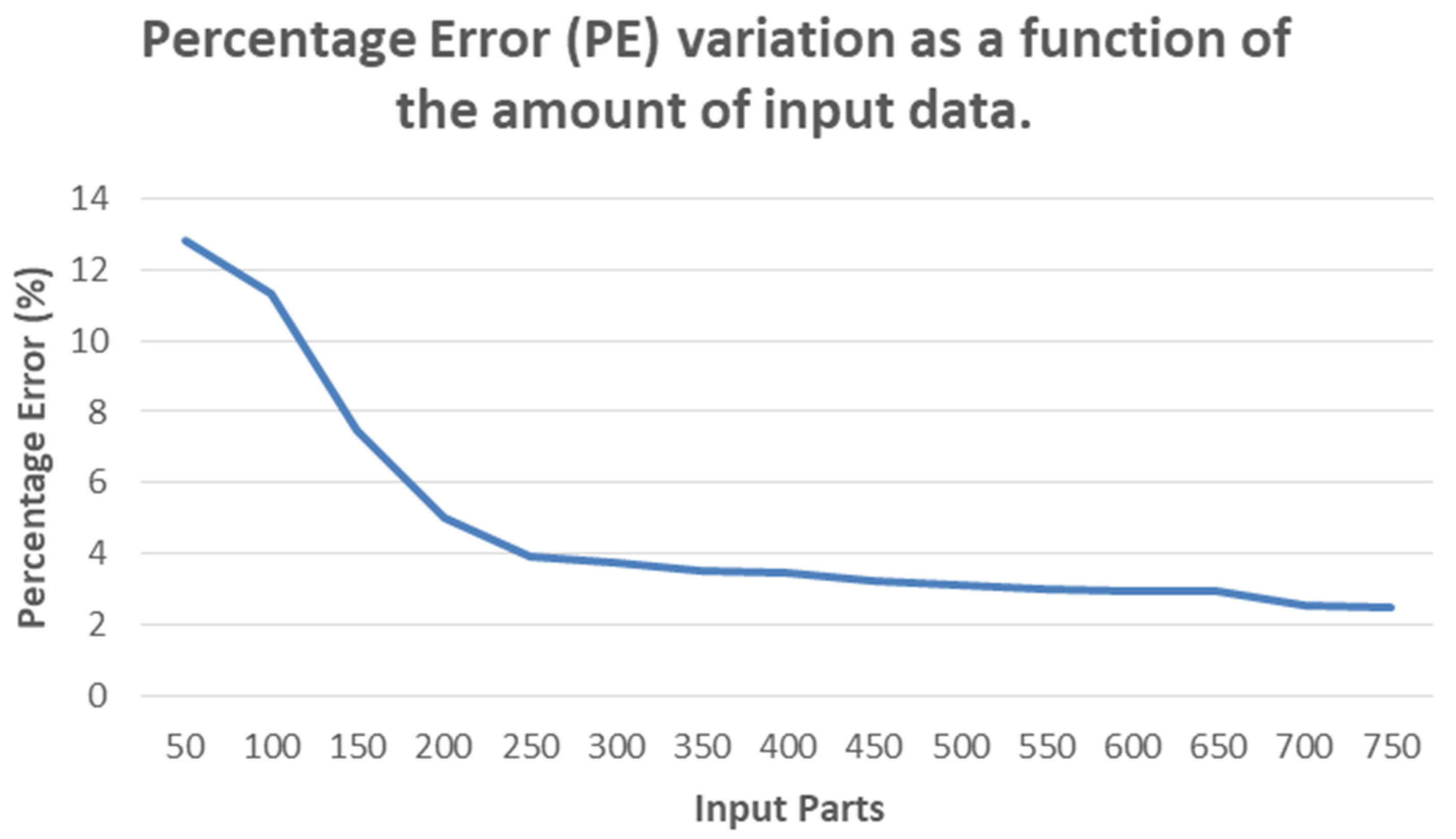
- It was observed that the R value would increase with an increase in number of considered parts. It was noted that this value would stabilize at around 250 parts.
The graph in Figure 5 shows the percentage error variation as a function of the number of input data. The error decreases as the number of parts increases. From 250 parts onwards, the percentage error is reduced to a lesser extent.
3.3. Test 3—Influence of Input Variables
From the application of the ANNs of Test 3 to the ‘testdata’ database, where the input variables are studied, the ANN with the lowest ME was T3_07, with an ME of 0.21 min. The ANN with the lowest MAE was T3_01, with an MAE of 4.85 min. With an MSE of 41.42 min, T3_01 was the best ANN in this parameter. The smallest maximum error recorded was 20.20 min and occurred in T3_07. The ANN with the lowest percentage error was T3_01, like T1_07 and T2_15, with a PE of 2.52% (please see Table 5).
From the training of the networks for Test 3, it can be concluded that:
- The networks T3_01 and T3_07 are the ones that showed the best training sample results, exhibiting an R value of 0.99;
- The best R value obtained for validation samples was the one obtained for T3_01;
- The T3_01 network also showed the best R results for the training sample, with a value of 0.98;
- The networks that showed the best overall results (Total) were the T3_01 and the T3_07 networks, with a R value of 0.98.
4. Discussion
The results obtained with Test 2 allowed for concluding something already expected, namely, that by increasing the number of data provided to the ANN, the learning process leads to high accuracy results, and thus the amount of data introduced in the future should be even higher, allowing for more accurate predictions. This directly results from the observations of Table 4 and Figure 5. This trend was previously argued by Tay and Cao [56], namely, that ANN results depend to a large extent on the amount of data provided to the system, being a time-consuming task.
Based on the results previously described, it can be stated that many network architectures have provided very accurate results, with eight architectures showing errors lower than 3.15% (96.85% accuracy), which can be considered an excellent result in terms of machining cost prediction. This result is less than those previously obtained by other researchers [57], who reported average accuracies of about 98.5% using ANNs, which has been shown to be a more accurate method to detect the different blends of fuel than RSM (response surface methodology) methods. Moreover, another study [58] about predictions of AISI 1050 steel machining performance has shown that ANNs presented the most accurate prediction value (92.1%), which is below the accuracy provided by the eight different architectures used in this work. In that work [58], it remains clear that ANN can provide more accurate values than other prediction techniques, such as the adaptive neuro-fuzzy inference system (ANFIS), which provided an accuracy of 73% compared to the 92.1% achieved using ANN. Saric et al. [55] also claimed an error of 2.03% using back-propagation neural networks in the estimation of CNC machining times. However, using self-organizing map neural networks, the results are less accurate, showing errors of about 10.05%. Ning et al. [52] used as a training dataset 21,943 features, and 4338 for validation, obtaining an accuracy of 97.7%, which is very similar to that achieved through this work. Thus, it is expected that a higher number of features used for training of the model can contribute to a better accuracy of the predictions, but too much data cannot contribute to accuracy improvement and can cause higher computing time, which can be unnecessary.
Regarding Table 5, the best results were obtaining using as input variables the volume of removed materials (V) and the total number of elements of each feature (Q). Indeed, the second most accurate result was obtained using the same variables plus the machined surface area (A). However, adding this variable, the results started to degrade. Among the other combinations considered in this work, only the Q + A combination presented acceptable results, together with the combination Q + At. Thus, it is possible to infer that the volume of removed materials plays an important role in terms of keeping the accuracy as high as possible, which can be combined with V for the best results and combined with A for close to the best results.
5. Conclusions
This work allowed us to analyze, study, and test the applicability of artificial neural networks in estimating machining times. One of the main contributions of the presented work is the development of an ANN that predicts the machining time of standard parts for plastic injection molds with a percent error of 2.52%.
The application of ANNs in this work proved to be a quick and efficient way to estimate machining times. The introduction of the total quantity and volume of each of the most common features regarding the standard parts proved to be sufficient for this purpose, and it was not necessary to detail individually in the training of the networks the dimensions of each element to be machined. The specification of each element to be machined would make the presented method slower, which would not meet the proposed goals.
The different tests carried out demonstrated that:
- Network architectures had a minor influence on the accuracy of ANNs;
- The amount of data used in network training proved to be of great importance. The ANNs trained with a more significant number of data had a lower percentage of error and better training values. However, excessive amounts of data were time-consuming in terms of computing and did not generate significant gains in terms of accuracy;
- The decrease in the percentage of error of the trained network was less accentuated as the number of data used in training increased;
- The volume of removed material and the total number of elements to be machined proved to be the input variables that provided the lowest percentage error, i.e., the best accuracy of predicted machining costs;
- Contrary to what would be expected, the introduction of the area to the quantity and volume of each group of elements did not represent a decrease in the percentage error;
- The variables total amount of elements to machine, total volume to machine, and the total area to machine did not show good results. This fact indicates that it is necessary to at least group the elements to be machined in similar groups;
- In all tests, a good relationship was confirmed between the regression results of the network training and the percentage error results.
The present work brings new knowledge about the possibility of applying ANNs in the estimation of machining times, which is not very common in the recently analyzed literature. This enables the use of these methods in industry sectors, such as the mold industry, enabling the determination of the machining time and overall production cost of standardized mold parts. However, there are some current limitations of the proposed work. This study was developed for an application regarding the production of mold parts, and although this methodology can be employed in other industry sectors (particularly machining sectors of standardized parts), this would involve calibration and training of new ANNs. Despite this fact, this work highlights the use of ANNs compared to more time-consuming and expensive alternatives when determining operation times and costs.
Supplementary Materials
The following supporting information can be downloaded at: https://www.mdpi.com/article/10.3390/met12101709/s1, Figure S1: List of produced parts.
Author Contributions
A.R.: investigation, formal analysis and writing—review and editing; F.J.G.S.: conceptualization, methodology, project administration, resources, supervision and writing—review and editing; V.F.C.S.: formal analysis, validation, visualization and writing—review and editing; A.G.P.: formal analysis, validation and writing—review and editing; L.P.F.: formal analysis, validation and writing—review and editing; T.P.: formal analysis, validation and writing—review and editing. All authors have read and agreed to the published version of the manuscript.
Funding
This research received no external funding.
Institutional Review Board Statement
Not applicable.
Informed Consent Statement
Not applicable.
Data Availability Statement
No data is made available regarding this work.
Acknowledgments
Authors thank INEGI—Institute of Science and Innovation in Mechanical and Industrial Engineering for its support.
Conflicts of Interest
The authors declare no conflict of interest.
References
- Matarrese, P.; Fontana, A.; Sorlini, M.; Diviani, L.; Specht, I.; Maggi, A. Estimating energy consumption of injection moulding for environmental-driven mould design. J. Clean. Prod. 2017, 168, 1505–1512. [Google Scholar] [CrossRef]
- Oropallo, W.; Piegl, L.A. Ten challenges in 3D printing. Eng. Comput. 2016, 32, 135–148. [Google Scholar] [CrossRef]
- Altan, T.; Lilly, B.; Yen, Y.C. Manufacturing of dies and molds. CIRP Ann. Manuf. Technol. 2001, 50, 404–422. [Google Scholar] [CrossRef]
- Costa, C.; Silva, F.; Gouveia, R.M.; Martinho, R. Development of hydraulic clamping tools for the machining of complex shape mechanical components. Procedia Manuf. 2018, 17, 563–570. [Google Scholar] [CrossRef]
- Hällgren, S.; Pejryd, L.; Ekengren, J. Additive Manufacturing and High Speed Machining -cost Comparison of short Lead Time Manufacturing Methods. Procedia CIRP 2016, 50, 384–389. [Google Scholar] [CrossRef] [Green Version]
- Rao, R.V.; Kalyankar, V. Optimization of modern machining processes using advanced optimization techniques: A review. Int. J. Adv. Manuf. Technol. 2014, 73, 1159–1188. [Google Scholar] [CrossRef]
- Sousa, V.F.C.; Silva, F.J.G. Recent Advances in Turning Processes Using Coated Tools—A Comprehensive Review. Metals 2020, 10, 170. [Google Scholar] [CrossRef] [Green Version]
- Sousa, V.F.C.; Silva, F.J.G. Recent Advances on Coated Milling Tool Technology—A Comprehensive Review. Coatings 2020, 10, 235. [Google Scholar] [CrossRef] [Green Version]
- Silva, F.J.G.; Martinho, R.P.; Martins, C.; Lopes, H.; Gouveia, R.M. Machining GX2CrNiMoN26-7-4 DSS alloy: Wear analysis of TiAlN and TiCN/Al2O3/TiN coated carbide tools behavior in rough end milling operations. Coatings 2019, 9, 392. [Google Scholar] [CrossRef] [Green Version]
- Martinho, R.P.; Silva, F.J.G.; Martins, C.; Lopes, H. Comparative study of PVD and CVD cutting tools performance in milling of duplex stainless steel. Int. J. Adv. Manuf. Technol. 2019, 102, 2423–2439. [Google Scholar] [CrossRef]
- Thorenz, B.; Oßwald, F.; Schötz, S.; Westermann, H.-H.; Döpper, F. Applying and Producing Indexable End Mills: A Comparative Market Study in Context of Resource Efficiency. Procedia Manuf. 2020, 43, 167–174. [Google Scholar] [CrossRef]
- Sousa, V.F.C.; Silva, F.J.G.; Fecheira, J.S.; Lopes, H.M.; Martinho, R.P.; Casais, R.B.; Ferreira, L.P. Cutting forces assessment in cnc machining processes: A criticalreview review. Sensors 2020, 20, 4536. [Google Scholar] [CrossRef] [PubMed]
- Tlhabadira, I.; Daniyan, I.; Masu, L.; Mpofu, K. Development of a model for the optimization of energy consumption during the milling operation of titanium alloy (Ti6Al4V). Mater. Today Proc. 2021, 38, 614–620. [Google Scholar] [CrossRef]
- Zhang, X.; Yu, T.; Dai, Y.; Qu, S.; Zhao, J. Energy consumption considering tool wear and optimization of cutting parameters in micro milling process. Int. J. Mech. Sci. 2020, 178, 105628. [Google Scholar] [CrossRef]
- Xiao, Y.; Jiang, Z.; Gu, Q.; Yan, W.; Wang, R. A novel approach to CNC machining center processing parameters optimization considering energy-saving and low-cost. J. Manuf. Syst. 2021, 59, 535–548. [Google Scholar] [CrossRef]
- Westermann, H.-H.; Kafara, M.; Steinhilper, R. Development of a Reference Part for the Evaluation of Energy Efficiency in Milling Operations. Procedia CIRP 2015, 26, 521–526. [Google Scholar] [CrossRef]
- Gouveia, R.M.; Silva, F.J.G.; Reis, P.; Baptista, A.P.M. Machining Duplex Stainless Steel: Comparative Study Regarding End Mill Coated Tools. Coatings 2016, 6, 51. [Google Scholar] [CrossRef] [Green Version]
- Huang, N.; Jin, Y.; Lu, Y.; Yi, B.; Li, X.; Wu, S. Spiral toolpath generation method for pocket machining. Comput. Ind. Eng. 2020, 139, 106142. [Google Scholar] [CrossRef]
- Cafieri, S.; Monies, F.; Mongeau, M.; Bes, C. Plunge milling time optimization via mixed-integer nonlinear programming. Comput. Ind. Eng. 2016, 98, 434–445. [Google Scholar] [CrossRef] [Green Version]
- Wu, L.; Li, C.; Tang, Y.; Yi, Q. Multi-objective Tool Sequence Optimization in 2.5D Pocket CNC Milling for Minimizing Energy Consumption and Machining Cost. Procedia CIRP 2017, 61, 529–534. [Google Scholar] [CrossRef]
- Silva, J.; Silva, F.J.G.; Campilho, R.D.S.G.; Sá, J.C.; Ferreira, L.P. A Model for Productivity Improvement on Machining of Components for Stamping Dies. Int. J. Ind. Eng. Manag. 2021, 12, 85–101. [Google Scholar] [CrossRef]
- Michalik, P.; Zajac, J.; Hatala, M.; Mital, D.; Fecova, V. Monitoring surface roughness of thin-walled components from steel C45 machining down and up milling. Measurement 2014, 58, 416–428. [Google Scholar] [CrossRef]
- Li, Y.W.; Sun, Y.S.; Zhou, X.G. Theoretical Analysis and Experimental Verification that Influence Factors of Climb and Conventional Milling on Surface Roughness. Appl. Mech. Mater. 2013, 459, 407–412. [Google Scholar] [CrossRef]
- Hadi, M.; Ghani, J.; Haron, C.C.; Kasim, M.S. Comparison between Up-milling and Down-milling Operations on Tool Wear in Milling Inconel 718. Procedia Eng. 2013, 68, 647–653. [Google Scholar] [CrossRef] [Green Version]
- Bouzakis, K.D.; Makrimallakis, S.; Skordaris, G.; Bouzakis, E.; Kombogiannis, S.; Katirtzoglou, G.; Maliaris, G. Coated tools’ performance in up and down milling stainless steel, explained by film mechanical and fatigue properties. Wear 2013, 303, 546–559. [Google Scholar] [CrossRef]
- Agarwal, V.; Agarwal, S. Performance profiling of solid lubricant for eco-friendly sustainable manufacturing. J. Manuf. Process. 2021, 64, 294–305. [Google Scholar] [CrossRef]
- Makhesana, M.; Patel, K.; Mawandiya, B. Environmentally conscious machining of Inconel 718 with solid lubricant assisted minimum quantity lubrication. Met. Powder Rep. 2020, 76, S24–S29. [Google Scholar] [CrossRef]
- Agrawal, C.; Wadhwa, J.; Pitroda, A.; Pruncu, C.I.; Sarikaya, M.; Khanna, N. Comprehensive analysis of tool wear, tool life, surface roughness, costing and carbon emissions in turning Ti–6Al–4V titanium alloy: Cryogenic versus wet machining. Tribol. Int. 2021, 153, 106597. [Google Scholar] [CrossRef]
- Kumar, S.; Campilho, R.; Silva, F. Rethinking modular jigs’ design regarding the optimization of machining times. Procedia Manuf. 2019, 38, 876–883. [Google Scholar] [CrossRef]
- Kumar, S.R.; Krishnaa, D.; Gowthamaan, K.; Mouli, D.C.; Chakravarthi, K.C.; Balasubramanian, T. Development of a Re-engineered fixture to reduce operation time in a machining process. Mater. Today Proc. 2020, 37, 3179–3183. [Google Scholar] [CrossRef]
- Fiorentino, A. Cost drivers-based method for machining and assembly cost estimations in mould manufacturing. Int. J. Adv. Manuf. Technol. 2014, 70, 1437–1444. [Google Scholar] [CrossRef]
- Bouaziz, Z.; Ben Younes, J.; Zghal, A. Cost estimation system of dies manufacturing based on the complex machining features. Int. J. Adv. Manuf. Technol. 2006, 28, 262–271. [Google Scholar] [CrossRef]
- Narita, H. A Study of Automatic Determination of Cutting Conditions to Minimize Machining Cost. Procedia CIRP 2013, 7, 217–221. [Google Scholar] [CrossRef] [Green Version]
- Deng, S.; Yeh, T.-H. Using least squares support vector machines for the airframe structures manufacturing cost estimation. Int. J. Prod. Econ. 2011, 131, 701–708. [Google Scholar] [CrossRef]
- Loyer, J.-L.; Henriques, E.; Fontul, M.; Wiseall, S. Comparison of Machine Learning methods applied to the estimation of manufacturing cost of jet engine components. Int. J. Prod. Econ. 2016, 178, 109–119. [Google Scholar] [CrossRef]
- Lee, S.; Cho, Y.; Lee, Y.H. Injection Mold Production Sustainable Scheduling Using Deep Reinforcement Learning. Sustainability 2020, 12, 8718. [Google Scholar] [CrossRef]
- Viharos, Z.J.; Mikó, B. Artificial neural network approach for injection mould cost estimation. In Proceedings of the 44th CIRP Conference on Manufacturing Systems, Madison, WI, USA, 1–3 June 2009; pp. 1–6. [Google Scholar]
- Tansel, I.; Ozcelik, B.; Bao, W.; Chen, P.; Rincon, D.; Yang, S.; Yenilmez, A. Selection of optimal cutting conditions by using GONNS. Int. J. Mach. Tools Manuf. 2006, 46, 26–35. [Google Scholar] [CrossRef]
- De Filippis, L.A.C.; Serio, L.M.; Facchini, F.; Mummolo, F.F.A.G. ANN Modelling to Optimize Manufacturing Process. In Advanced Applications for Artificial Neural Networks; El-Shahat, A., Ed.; Intechopen: London, UK, 2018. [Google Scholar] [CrossRef] [Green Version]
- Mundada, V.; Narala, S.K.R. Optimization of Milling Operations Using Artificial Neural Networks (ANN) and Simulated Annealing Algorithm (SAA). Mater. Today Proc. 2018, 5, 4971–4985. [Google Scholar] [CrossRef]
- Chen, Y.; Sun, R.; Gao, Y.; Leopold, J. A nested-ANN prediction model for surface roughness considering the effects of cutting forces and tool vibrations. Measurement 2017, 98, 25–34. [Google Scholar] [CrossRef]
- Hesser, D.F.; Markert, B. Tool wear monitoring of a retrofitted CNC milling machine using artificial neural networks. Manuf. Lett. 2019, 19, 1–4. [Google Scholar] [CrossRef]
- El-Mounayri, H.; Briceno, J.F.; Gadallah, M. A new artificial neural network approach to modeling ball-end milling. Int. J. Adv. Manuf. Technol. 2010, 47, 527–534. [Google Scholar] [CrossRef]
- Al-Abdullah, K.I.A.-L.; Abdi, H.; Lim, C.P.; Yassin, W.A. Force and temperature modelling of bone milling using artificial neural networks. Measurement 2018, 116, 25–37. [Google Scholar] [CrossRef]
- Zain, A.M.; Haron, H.; Sharif, S. Genetic Algorithm and Simulated Annealing to estimate optimal process parameters of the abrasive waterjet machining. Eng. Comput. 2011, 27, 251–259. [Google Scholar] [CrossRef] [Green Version]
- Mohanraj, T.; Shankar, S.; Rajasekar, R.; Sakthivel, N.R.; Pramanik, A. Tool condition monitoring techniques in milling process—A review. J. Mater. Res. Technol. 2020, 9, 1032–1042. [Google Scholar] [CrossRef]
- Serin, G.; Sener, B.; Ozbayoglu, A.M.; Unver, H.O. Review of tool condition monitoring in machining and opportunities for deep learning. Int. J. Adv. Manuf. Technol. 2020, 109, 953–974. [Google Scholar] [CrossRef]
- Kuntoğlu, M.; Aslan, A.; Pimenov, D.Y.; Usca, Ü.A.; Salur, E.; Gupta, M.K.; Mikolajczyk, T.; Giasin, K.; Kapłonek, W.; Sharma, S. A Review of Indirect Tool Condition Monitoring Systems and Decision-Making Methods in Turning: Critical Analysis and Trends. Sensors 2021, 21, 108. [Google Scholar] [CrossRef]
- Pimenov, D.Y.; Bustillo, A.; Wojciechowski, S.; Sharma, V.S.; Gupta, M.K.; Kuntoğlu, M. Artificial intelligence systems for tool condition monitoring in machining: Analysis and critical review. J. Intell. Manuf. 2022, 1–43. [Google Scholar] [CrossRef]
- Kataraki, P.S.; Abu Mansor, M.S. Automatic designation of feature faces to recognize interacting and compound volumetric features for prismatic parts. Eng. Comput. 2020, 36, 1499–1515. [Google Scholar] [CrossRef]
- Ning, F.; Shi, Y.; Cai, M.; Xu, W.; Zhang, X. Manufacturing cost estimation based on the machining process and deep-learning method. J. Manuf. Syst. 2020, 56, 11–22. [Google Scholar] [CrossRef]
- Atia, M.R.; Khalil, J.; Mokhtar, M. A Cost estimation model for machining operations.; an ann parametric approach. J. Al-Azhar Univ. Eng. Sect. 2017, 12, 878–885. [Google Scholar] [CrossRef] [Green Version]
- Florjanič, B.; Kuzman, K. Estimation of time for manufacturing of injection moulds using artificial neural networks-based model. Polim. Časopis Plast. Gumu 2012, 33, 12–21. [Google Scholar]
- Yoo, S.; Kang, N. Explainable artificial intelligence for manufacturing cost estimation and machining feature visualization. Expert Syst. Appl. 2021, 183, 115430. [Google Scholar] [CrossRef]
- Saric, T.; Simunovic, G.; Simunovic, K. Estimation of Machining Time for CNC Manufacturing Using Neural Computing. Int. J. Simul. Model. 2016, 15, 663–675. [Google Scholar] [CrossRef]
- Tay, F.E.; Cao, L. Application of support vector machines in financial time series forecasting. Omega 2001, 29, 309–317. [Google Scholar] [CrossRef]
- Mahmodi, K.; Mostafaei, M.; Mirzaee-Ghaleh, E. Detecting the different blends of diesel and biodiesel fuels using electronic nose machine coupled ANN and RSM methods. Sustain. Energy Technol. Assess. 2022, 51, 101914. [Google Scholar] [CrossRef]
- Sada, S.; Ikpeseni, S. Evaluation of ANN and ANFIS modeling ability in the prediction of AISI 1050 steel machining performance. Heliyon 2021, 7, e06136. [Google Scholar] [CrossRef]
Figure 1.
Diagram of the input variables of the proposed solution.

Figure 2.
Examples of models used to produce the mold parts (Figure S1).
Figure 2.
Examples of models used to produce the mold parts (Figure S1).

Figure 3.
Machining times of each of the 30 parts obtained by the traditional method (TM) and the empirical method (EM).
Figure 3.
Machining times of each of the 30 parts obtained by the traditional method (TM) and the empirical method (EM).

Figure 4.
Traditional method (a) and empirical method (b) machining time in percentage (Ct—cutting time; Rt—rapid travelling time).
Figure 4.
Traditional method (a) and empirical method (b) machining time in percentage (Ct—cutting time; Rt—rapid travelling time).

Figure 5.
Percentage error (PE) variation as a function of the amount of input data.


Table 1.
Feature definitions and corresponding sequences of operations.
| Feature Group | Illustration | A (mm) | B (mm) | C (mm) | D (mm) | Sequence of Operations |
|---|---|---|---|---|---|---|
| Metric threads |  | M3; M4; M5; M6; M8; M10; M12; M16; M20; M24; M30. | -- | -- | -- | 1st—Drill; 2nd—Chamfer; 3rd—Tap. |
| Clearance holes |  | 6.00; 7.00; 9.00; 10.00; 11.00; 11.50; 13.50; 14.00; 15.50; 16.00; 17.50; 20.00; 22.00; 22.50; 27.00. | 46.00; | -- | -- | 1st—Drill; 2nd—Chamfer. |
| 66.00; | ||||||
| 86.00; | ||||||
| 96.00; | ||||||
| 136.00. | ||||||
| Screw clearance holes |  | 10.00; 11.00; 14.00; 17.00; 21.00; 23.00; 26.00; 32.00; 37.00. | 6.00; 7.00; 9.00; 11.00; 13.50; 15.50; 17.50; 21.00; 27.00. | 6.00; 7.00; 9.00; 11.00; 13.00; 15.00; 17.00; 21.00; 27.00. | 46.00; | 1st—Drill; 2nd—Counter-boring; 3rd—Chamfer. |
| 66.00; | ||||||
| 86.00; | ||||||
| 96.00; | ||||||
| 136.00. | ||||||
| Fitting holes |  | 10.00; 12.00; 16.00; 20.00. | 10.00; 16.00; 25.00; 30.00. | -- | -- | 1st—Drill; 2nd—Bore; 3rd—Chamfer. |
Table 2.
Tool steels used to calculate machining time.
| Material No. | AISI | DIN |
|---|---|---|
| 1.1730 | 1045 | C45E |
| 1.2311 | P20 | 40CrMnMo7 |
Table 3.
Regression and error of the ANNs from Test 1.
| Test | Arch. | R | Error | |||||||
|---|---|---|---|---|---|---|---|---|---|---|
| Train | Validation | Test | Total | ME (min) | MAE (min) | MSE (min) | EMax (min) | PE (%) | ||
| T1_01 | 4-8-1 | 0.98 | 0.97 | 0.98 | 0.98 | 0.16 | 5.00 | 42.22 | 17.14 | 2.63 |
| T1_02 | 4-4-1 | 0.94 | 0.93 | 0.85 | 0.93 | −1.82 | 8.40 | 221.91 | 71.23 | 6.15 |
| T1_03 | 4-9-1 | 0.99 | 0.98 | 0.97 | 0.98 | 0.57 | 4.74 | 38.72 | 23.13 | 2.78 |
| T1_04 | 4-10-1 | 0.98 | 0.98 | 0.96 | 0.98 | 1.95 | 5.31 | 43.74 | 15.30 | 2.86 |
| T1_05 | 4-15-1 | 0.98 | 0.97 | 0.98 | 0.98 | 0.16 | 5.37 | 47.20 | 21.72 | 2.89 |
| T1_06 | 4-20-1 | 0.98 | 0.97 | 0.98 | 0.98 | 1.38 | 5.20 | 45.47 | 19.54 | 2.66 |
| T1_07 | 4-8-8-1 | 0.99 | 0.99 | 0.98 | 0.98 | 0.26 | 4.85 | 41.42 | 25.71 | 2.52 |
| T1_08 | 4-10-10-1 | 0.99 | 0.98 | 0.97 | 0.98 | −0.66 | 5.57 | 62.06 | 37.06 | 2.88 |
| T1_09 | 4-4-4-1 | 0.97 | 0.96 | 0.96 | 0.97 | 2.09 | 6.62 | 75.98 | 34.69 | 3.13 |
Table 4.
Regression and error of the ANNs from Test 2.
| Test | Input Parts | R | Error | |||||||
|---|---|---|---|---|---|---|---|---|---|---|
| Train | Validation | Test | Total | ME (min) | MAE (min) | MSE (min) | EMax (min) | PE (%) | ||
| T2_01 | 50 | 0.63 | 0.86 | 0.90 | 0.67 | 2.45 | 21.64 | 799.52 | 78.15 | 12.82 |
| T2_02 | 100 | 0.85 | 0.74 | 0.66 | 0.82 | 6.74 | 23.99 | 906.34 | 96.35 | 11.29 |
| T2_03 | 150 | 0.97 | 0.88 | 0.93 | 0.96 | 2.69 | 12.50 | 265.21 | 46.08 | 7.48 |
| T2_04 | 200 | 0.97 | 0.97 | 0.93 | 0.97 | −0.32 | 9.47 | 175.14 | 44.10 | 5.01 |
| T2_05 | 250 | 0.98 | 0.96 | 0.98 | 0.98 | 0.43 | 6.94 | 85.75 | 37.75 | 3.95 |
| T2_06 | 300 | 0.98 | 0.97 | 0.97 | 0.97 | −0.29 | 6.95 | 81.23 | 33.91 | 3.78 |
| T2_07 | 350 | 0.99 | 0.95 | 0.97 | 0.98 | −1.16 | 6.27 | 62.82 | 23.14 | 3.55 |
| T2_08 | 400 | 0.98 | 0.97 | 0.96 | 0.98 | −1.35 | 6.43 | 67.74 | 24.18 | 3.49 |
| T2_09 | 450 | 0.99 | 0.98 | 0.97 | 0.98 | −0.96 | 5.85 | 52.05 | 16.73 | 3.26 |
| T2_10 | 500 | 0.98 | 0.97 | 0.98 | 0.98 | 1.42 | 5.59 | 54.26 | 25.16 | 3.15 |
| T2_11 | 550 | 0.98 | 0.98 | 0.98 | 0.98 | 1.80 | 5.72 | 57.80 | 27.27 | 2.99 |
| T2_12 | 600 | 0.99 | 0.97 | 0.97 | 0.98 | 0.62 | 5.27 | 45.28 | 22.02 | 2.98 |
| T2_13 | 650 | 0.99 | 0.98 | 0.98 | 0.99 | −0.08 | 5.49 | 55.31 | 27.80 | 2.98 |
| T2_14 | 700 | 0.98 | 0.98 | 0.97 | 0.98 | 0.27 | 4.88 | 40.18 | 17.09 | 2.57 |
| T2_15 | 750 | 0.99 | 0.99 | 0.98 | 0.98 | 0.26 | 4.85 | 41.42 | 25.71 | 2.52 |
Table 5.
Regression and error of the ANNs from Test 3.
| Test | Input Variables | R | Error | |||||||
|---|---|---|---|---|---|---|---|---|---|---|
| Train | Validation | Test | Total | ME (min) | MAE (min) | MSE (min) | EMax (min) | PE (%) | ||
| T3_01 | Q + V | 0.99 | 0.99 | 0.98 | 0.98 | 0.26 | 4.85 | 41.42 | 25.71 | 2.52 |
| T3_02 | Q + A | 0.96 | 0.95 | 0.95 | 0.95 | 2.13 | 8.90 | 143.17 | 42.02 | 4.58 |
| T3_03 | V + A | 0.97 | 0.95 | 0.97 | 0.97 | −2.76 | 6.65 | 68.63 | 23.18 | 3.21 |
| T3_04 | QT + VT | 0.72 | 0.76 | 0.74 | 0.73 | 1.89 | 18.85 | 600.44 | 67.70 | 10.26 |
| T3_05 | QT + AT | 0.79 | 0.81 | 0.85 | 0.80 | 30.06 | 31.46 | 1373.17 | 91.06 | 14.66 |
| T3_06 | VT + AT | 0.83 | 0.83 | 0.84 | 0.83 | 25.90 | 27.23 | 1154.57 | 105.98 | 12.54 |
| T3_07 | Q + V + A | 0.99 | 0.98 | 0.97 | 0.98 | 0.21 | 5.74 | 52.53 | 20.20 | 2.77 |
| T3_08 | Q + VT | 0.89 | 0.85 | 0.86 | 0.88 | 18.37 | 19.17 | 561.75 | 67.30 | 8.44 |
| T3_09 | Q + AT | 0.93 | 0.93 | 0.94 | 0.93 | 1.80 | 8.98 | 133.10 | 32.55 | 4.43 |
Publisher’s Note: MDPI stays neutral with regard to jurisdictional claims in published maps and institutional affiliations. |
© 2022 by the authors. Licensee MDPI, Basel, Switzerland. This article is an open access article distributed under the terms and conditions of the Creative Commons Attribution (CC BY) license (https://creativecommons.org/licenses/by/4.0/).
Share and Cite
MDPI and ACS Style
Rodrigues, A.; Silva, F.J.G.; Sousa, V.F.C.; Pinto, A.G.; Ferreira, L.P.; Pereira, T. Using an Artificial Neural Network Approach to Predict Machining Time. Metals 2022, 12, 1709. https://doi.org/10.3390/met12101709
AMA Style
Rodrigues A, Silva FJG, Sousa VFC, Pinto AG, Ferreira LP, Pereira T. Using an Artificial Neural Network Approach to Predict Machining Time. Metals. 2022; 12(10):1709. https://doi.org/10.3390/met12101709
Chicago/Turabian StyleRodrigues, André, Francisco J. G. Silva, Vitor F. C. Sousa, Arnaldo G. Pinto, Luís P. Ferreira, and Teresa Pereira. 2022. "Using an Artificial Neural Network Approach to Predict Machining Time" Metals 12, no. 10: 1709. https://doi.org/10.3390/met12101709
Note that from the first issue of 2016, this journal uses article numbers instead of page numbers. See further details here.