A Simulation-Based Digital Design Methodology for Studying Conjugate Heat Transfer in Tundish

Abstract

The successful design of refractory lining for a tundish is critical due to the demand of superheat control, improvement of steel cleanliness and reduction in material cost during continuous casting. A design of experiment analysis, namely, the Taguchi method, was employed to analyze two-dimensional heat transfer through refractory linings of a single-strand tundish, with the consideration of the thickness and the thermal conductivity of lining materials. In addition, a three-dimensional conjugate heat transfer model was applied in the tundish, taking in account the molten steel flow and heat conduction in the linings. A special focus of this study was to demonstrate the analysis methodology of combining Taguchi and CFD modelling to explore lining design in terms of thickness and thermal conductivity for the given process conditions during tundish operations.

1. Introduction

Continuous casting tundish, working as a buffer and distributor of liquid steel between the ladle and continuous casting molds, plays a key role in affecting the performance of casting and solidification, as well as the quality of final products, referred to as “Tundish Metallurgy”. Considerable research efforts have been made in academia and industry over many decades to fully exploit and enhance the metallurgical performance of the tundish [1,2,3,4].

Refractory linings of the tundish are designed to prevent heat loss, withstand thermal shock and resist erosion. In addition, it is also important to prevent the molten steel getting contaminated with unwanted impurities. A typical tundish refractory lining has three solid layers, including (i) insulation layer, (ii) permanent layer, and (iii) working layer. The insulation lining is a layer adjacent to steel shell, reducing the heat loss and thermomechanical loads at the hot surface of the working lining. The permanent lining is next to the insulation layer with the main role of safety insulation. The working lining is in direct contact with molten steel during the casting process. The working lining material should have good high-temperature performance and good chemical stability [5,6,7].

A typical tundish usage cycle consists of construction, preheating, steel casting, cooling, removal of skull, and repair. Tundish preheating can be applied for drying and heating of an empty tundish, which plays an important role for the entire casting process. For tundish drying, it is required to remove the moisture from a newly lined (green) tundish for the control of hydrogen content in molten steel. A long drying process with a slow heating rate is necessary to ensure that the refractory is subjected to a minimum of thermal shocks. For tundish heating, it is required to heat the tundish at a fast rate before taping of the ladle. The burner provides a high heating rate from the flame to the lining in order to ensure that the tundish is fully soaked. The preheating process can minimize the thermal shock to the refractory lining and temperature drop in the tundish. However, overheating of a preheated tundish can also occur, resulting in costly energy losses and unwanted refractory damage. Therefore, it is necessary to investigate transient heat transfer and control thermal state of the refractory lining during the preheating process.

During the on-line steel casting process, the molten steel will be poured from the ladle into the tundish. There are conductive heat losses through the wall of a tundish and radiative heat loss through the bath surface. The tundish is heated up when filled with molten steel due to the heat absorbed from the melt by the refractory lining. To analyze heat transfer of molten steel in the study, CFD models are applied. The studied phenomena of the CFD model include residence time distribution [8,9,10], flow control device [11,12,13], inclusion behavior [14,15] and thermal status [16,17,18]. A series of CFD modelling studies have recently been published by the author and co-workers with the focus on developing a simulation-based digital design methodology to optimize the tundish geometry and process parameters during the casting process [19,20,21,22,23,24,25]. These modelling studies led to considerable improvements in understanding the various flow phenomena associated with the tundish operations.

Within the published tundish studies, very few performed studies considering a systematic variation of the thermal state of the tundish; for example, the boundary condition of the walls and the tundish surface was commonly set up as a constant heat loss in the CFD model. Under real production conditions, heat loss during casting varied on working conditions and thermal states of refractory linings. Detailed quantitative analysis for the thermal state of refractory lining and its effect on flow patterns in tundish have rarely been published.

In the present study, a conjugate heat transfer model was applied in a single-strand tundish, considering both molten steel flow and heat conduction through the refractor linings and steel shell. A design of experiment (DOE) analysis, namely, the Taguchi method, was employed to analyze the effects of thickness and thermal conductivity of the refractory lining on the thermal states of the tundish during casting operation. A special focus of this study was to demonstrate the capabilities of the combined Taguchi and CFD analysis as an effective tool for the analysis of fluid flow and heat transfer. The results for process optimization and energy saving will continue to encourage the application of the simulation-based digital design methodology in research and industrial design practice.

2. Model Description

2.1. Two-Dimensional Heat Transfer

Figure 1 shows the schematic diagram of the refractory lining structure in tundish. The refractory lining is four layered. It could be considered as a two-dimensional structure in the modelling process. Heat conduction is driven by the local temperature gradient, while convection is modelled using a temperature difference. In 2D heat transfer calculation, the refractory layer was considered as a four-layered system involving both conduction and convection, assuming a steady local heat flux through the system. A network model could be applied to thermal circuits (shown in Figure 1) [26]. The inverse of conductance of the thermal circuit across the network can be calculated according to Equation (1).

$$\frac{1}{h_t}=\frac{1}{h_1}+\frac{L_{Working}}{k_{Working}}+\frac{L_{Permanent}}{k_{Permanent}}+\frac{L_{Insulation}}{k_{Insuatlion}}+\frac{L_{Steel}}{k_{Steel}}+\frac{1}{h_5}$$

(1)

where h is heat transfer coefficient, k is heat conductivity of the solid layer, L is the thickness of the layer.

A constant temperature is used as the thermal boundary condition at the hot fluid side. At the cold fluid side, the heat loss is calculated based on heat transfer coefficient (18 W/m²K) and environment temperature (30 °C). The physical properties of refractory linings used in steel plant are listed in

Table 1. Physical properties of refractory linings.

Level Factor	ρ (kg∙m−3)	Cp (J∙kg−1 K−1)	Thermal Conductivity k (W∙m−1K−1)	Thickness L (m)
1. Working	1900	1090	3.42	0.05
2. Permanent	2860	800	2.10	0.15
3. Insulation	1200	816.4	0.15	0.05
4. Steel shell	7800	473	28.9	0.05

.

2.2. Taguchi and ANOVA Analysis

Minitab V.18 (Minitab, LLC, State College, Pennsylvania, PA, USA) software was used for design of experiment (DOE) analysis [27]. The DOE consists of four phases: planning, characterization, optimization, and verification. The optimization was built by combining CFD simulation and design of experiment.

Taguchi analysis uses a classical signal-to-noise (S/N) ratio as a numerical measurement for deciding the optimal circumstances. Noise (N) is the set of uncontrolled parameters that influences the result or response [28,29]. Signal (S) is the output variable or response. The S/N ratio indicates robustness of an experiment. There are three categories of S/N ratios: (i) smaller-is-better, (ii) larger-is-better, and (iii) nominal-is-best. The three S/N ratios are described in Equations (2)–(4). Depending on the application, one should firstly identify the objective function to be optimized.

$$\mathrm{smaller}-\mathrm{is}-\mathrm{better}: S/N=-10\log \left(\frac{1}{n}{\displaystyle \sum _{i=1}^n{y}_i^2}\right)$$

(2)

$$\mathrm{larger}-\mathrm{is}-\mathrm{better}: S/N=-10\log \left(\frac{1}{n}{\displaystyle \sum _{i=1}^n\frac{1}{y_i^2}}\right)$$

(3)

$$\mathrm{normal}-\mathrm{is}-\mathrm{best}: S/N=10\log \left(\frac{{\overline{y}}^2}{s^2}\right)$$

(4)

where y is the performance characteristic value, n is the observation repeat number, and s² is the variance.

In this work, the Taguchi orthogonal array L27 (6 factors and 3 levels) OA (orthogonal array) was applied to define the designs regarding the selected factors. In

Table 2. Controlled factors and levels.

Property	Factor	Unit	Level 1	Level 2	Level 3
Conductivity	A-working	W/mK	2.5650	3.4200	4.2750
	B-permanent	W/mK	1.5750	2.1000	2.6250
	C-insulation	W/mK	0.1125	0.1500	0.1880
Thickness	D-Working	m	0.0375	0.0500	0.0625
	E-Permanent	m	0.1125	0.1500	0.1875
	F-Insulation	m	0.0375	0.0500	0.0625

, six factors with high (level 3), medium (level 2), and low values (level 1) were considered in DOE. Level 3 and level 1 is plus/minus 25% from level 2, respectively. The data of level 2 are collected from the steel plant. It should be mentioned that the level setting was considered only for the mathematical modelling. The chemical compositions of refractory linings related to the material properties are not included in this study. As suggested by the Taguchi orthogonal array, twenty-seven CFD cases were proposed with different combinations of the factor levels and displayed in Table 4. Case 0 (normal condition) was added as a reference case.

ANOVA (Analysis of variance) is applied to determine the effects of independent variables (the various factors of interest) on the dependent variable (the response of physical phenomenon) in statistical analysis. This method is developed by Ronald Fisher, also referred to as the F-test [30]. It has two merits: (i) obtaining contribution rate of factors by analyzing the variation in factors, and (ii) verifying the results’ reliability by Taguchi analysis. The criteria for determining the effect of a design factor on response function mainly depends on the magnitude of the F-value. The design factor with the highest F-value represents the factor with the most significant effect on the response function. The mathematical description of the ANOVA, such as a sum of squares (SS), mean of squares (MS), degree of freedom (DOF), and F-values, are calculated using equations below.

Sum of Squares for Treatments,

$$SSR=n_{\mathrm{S}}{\displaystyle \sum _{i=1}^k{\left({\overline{y}}_i-\overline{\overline{y}}\right)}^2}$$

(5)

SSR is the “Between Group” variation, where the k “groups” or populations are represented by their sample means, $\overline{\overline{y}}$ is the mean of all n observations,

Sum of Squares for Error,

$$SSE={\displaystyle \sum _{i=1}^k{\displaystyle \sum _{j=1}^{n_S}{\left(y_{ij}-{\overline{y}}_i\right)}^2}}$$

(6)

SSE is the “Within Group” variation and represents the random or sample-to-sample variation.

Total Sum of Squares,

$$SST={\displaystyle \sum _{i=1}^k{\displaystyle \sum _{j=1}^{n_S}{\left(y_{ij}-\overline{\overline{y}}\right)}^2}}$$

(7)

SST is the total variation in the values of the response variables over all k samples.

Mean Square for Treatments,

$$MSR=\frac{SSR}{k-1}$$

(8)

Mean Square for Error,

$$MSE=\frac{SSE}{n-k}$$

(9)

Statistic used to test the null hypothesis (F-value):

$$F=\frac{MSR}{MSE}$$

(10)

where index i represents the ith population or treatment and the index j represents the jth observation within a sample, n is the total number of observations from all samples, y_ij is the value of the jth observation in the ith sample, and ${\overline{y}}_i$ is the mean of the ith sample.

2.3. Three-Dimensional Conjugate Heat Transfer

The CFD model with conjugate heat transfer (CHT) can simultaneously calculate the changes in fluid flow and the heat conduction in solid. The temperature and heat flux are exchanged at fluid–solid interface by the coupling methods at each numerical iteration. CFD software Siemens Simcenter STAR-CCM+ 2020.02 (Siemens Digital Industries Software, Plano, TX, USA) was used to calculate three-dimensional conjugate heat transfer and residence-time distribution of molten steel in tundish [31]. The assumptions made for the mathematical model are described below:

• The model is based on a 3D standard set of the Navier–Stokes equations.
• Both steady-state and transient liquid flow are considered.
• Fluid flow and heat transfer of molten steel are calculated.
• Boussinesq model is applied to calculate the natural convection flow.
• The heat conduction and heat losses through refractory lining are included.
• The free surface is flat and is kept at a fixed level. The slag layer is not included.

2.3.1. Transport Equation

Equations (11)–(13) describe an example set of the Navier–Stokes equations that govern the liquid phase [32].

Continuity:

$$\frac{\partial \rho }{\partial t}+\frac{\partial \left(\rho u_j\right)}{\partial x_j}=0$$

(11)

Momentum:

$$\rho \frac{\partial u_i}{\partial t}+\rho u_j\frac{\partial u_i}{\partial x_j}=-\frac{\partial P}{\partial x_i}+\frac{\partial }{\partial x_j}\left[\left(\mu +{\mu }_t\right)\left\{\frac{\partial u_i}{\partial x_j}+\frac{\partial u_j}{\partial x_i}\right\}\right]+g_i\left(\rho -{\rho }_0\right)$$

(12)

Thermal energy:

$$\rho C_p\frac{\partial T}{\partial t}+\rho C_p\frac{\partial \left(u_{j}T\right)}{\partial x_j}=\frac{\partial }{\partial x_j}\left[\left(k_0+\frac{C_p{\mu }_t}{P{r}_t}\right)\frac{\partial T}{\partial x_j}\right]+S_T$$

(13)

where ρ is the density; C_p is the heat capacity; µ_t is the turbulent viscosity; Pr_t is the turbulent Prandtl number (the value of 0.9). S_T represents the source term of energy equation.

Realizable k-ε model: [33]

$$\frac{\partial }{\partial t}\left(\rho k\right)+\frac{\partial }{\partial x_j}\left(\rho k{u}_j\right)=\frac{\partial }{\partial x_j}\left[\left(\mu +\frac{{\mu }_t}{{\sigma }_k}\right)\frac{\partial k}{\partial x_j}\right]+G_k+G_b-\rho \epsilon -Y_M+S_k$$

(14)

$$\frac{\partial }{\partial t}\left(\rho \epsilon \right)+\frac{\partial }{\partial x_j}\left(\rho \epsilon u_j\right)=\frac{\partial }{\partial x_j}\left[\left(\mu +\frac{{\mu }_t}{{\sigma }_{\epsilon }}\right)\frac{\partial \epsilon }{\partial x_j}\right]+\rho C_{1}S\epsilon -\rho C_2\frac{{\epsilon }^2}{k+\sqrt{v\epsilon }}+C_{1\epsilon }\frac{\epsilon }{k}{C}_3{G}_b+S_{\epsilon }$$

(15)

where k is the turbulent kinetic energy; ε is the turbulent energy dissipation rate; µ is the molecular viscosity; µ_t is the turbulent viscosity; G_k represents the generation of turbulent kinetic energy due to the mean velocity; Y_M represents the contribution of the fluctuating dilatation in compressible turbulence to the overall dissipation rate; υ is the kinematic viscosity; and σ_k and σ_ε are the turbulent Prandtl numbers for k and ε, respectively.

Two passive scalar equations are solved in the liquid region: (i) an instantaneous addition of the tracer at the inlet (E-curve); (ii) a continuous addition of tracers at inlet (F-curve). The passive scalar transport equations are solved at each time step once the fluid field is calculated.

$$\rho \frac{\partial \overline{C}}{\partial t}+\rho \overline{u_j}\frac{\partial \overline{C}}{\partial x_j}-\frac{\partial }{\partial x_j}\left[\rho D_{eff}\frac{\partial \overline{C}}{\partial x_j}\right]=0$$

(16)

where D_eff is the effective diffusivity. The velocity field is solved and obtained from a steady-state simulation and remained constant during the calculation of the passive scalar.

2.3.2. Analysis of RTD Curves

E-curve can be plotted based on the dimensionless outlet concentration (C-curve). Actual mean residence time is presented in Equation (17) [34].

$$\overline{\tau }=\frac{{{\displaystyle \int }}_0^{\infty }tC\left(t\right)dt}{{{\displaystyle \int }}_0^{\infty }C\left(t\right)dt}$$

(17)

The plug flow volume fraction (V_p/V), mixed flow volume fraction (V_m/V), and dead volume fraction (V_d/V) were calculated through Equations (18)–(20) [35].

Dead volume fraction,

$$V_{\mathrm{d}}/V=1-\frac{\overline{\tau }}{\tau }$$

(18)

Plug flow volume fraction,

$$V_{\mathrm{P}}/V=\left({\theta }_{\min }+{\theta }_{\mathrm{peak}}\right)/2$$

(19)

Mixed flow volume fraction,

$$V_{\mathrm{m}}/V=1-V_{\mathrm{d}}/V-V_{\mathrm{p}}/V$$

(20)

where τ is the theoretical residence time, θ_min is the dimensionless time of minimum concentration at the tundish outlet, θ_peak is the dimensionless time of peak concentration at the tundish outlet.

Another common RTD expression is the cumulative distribution function F(t), i.e., the F-curve. F-curve is a fraction of the liquid that has a residence time less than time (t) and can be obtained by making a continuous addition of tracers at the inlet. The concentration of tracers in the outlet stream is F-curve. In this study, F-curve was analyzed to evaluate an intermixing time exists between 0.2 and 0.8 of the dimensionless concentration of the tracer.

2.3.3. Geometry, Mesh, and Boundary Conditions

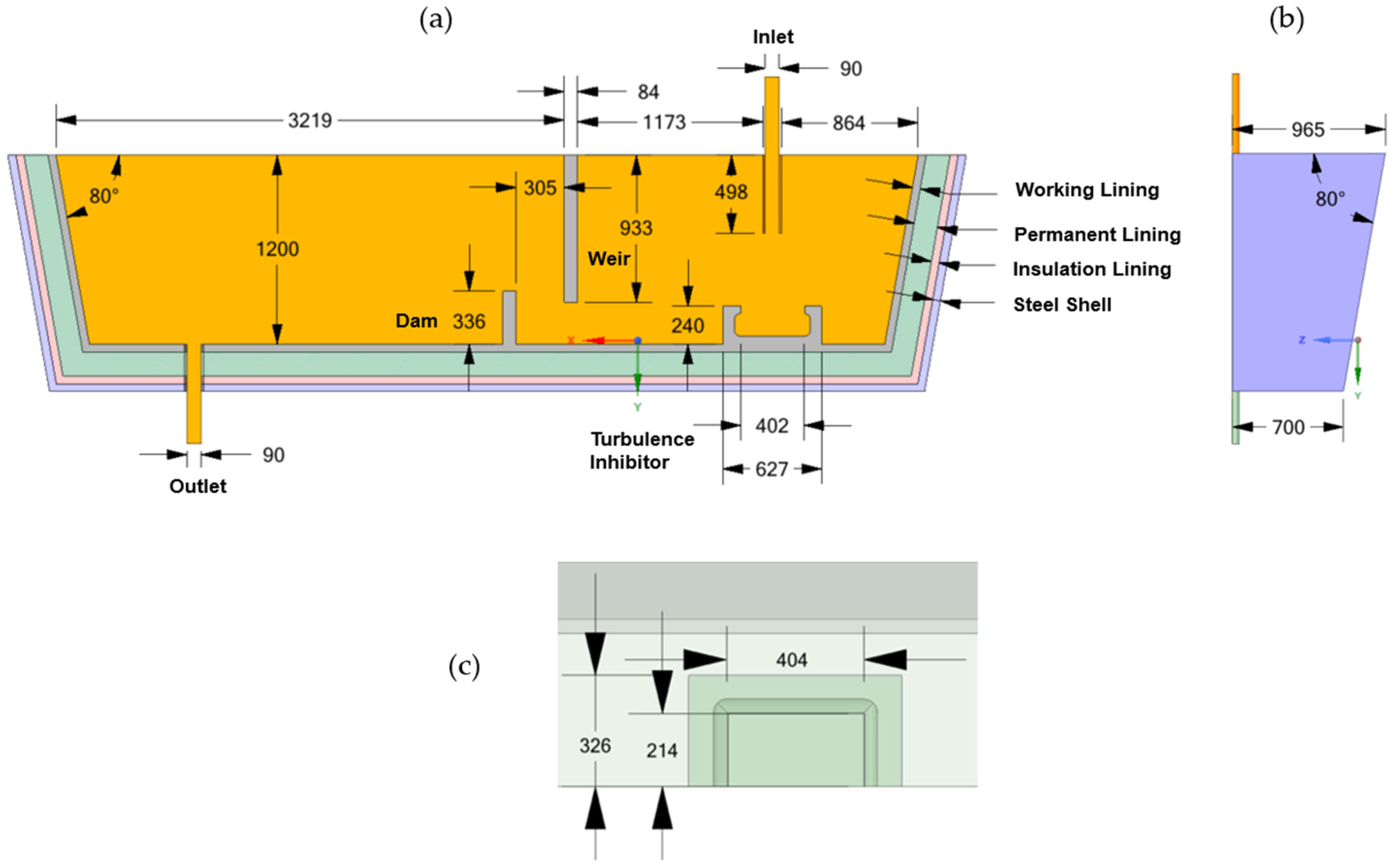
A single-strand tundish (48 tons), with a submerged inlet, an outlet, a weir, a dam and a turbulence inhibitor, was investigated in the current work. The geometric dimensions of the tundish are illustrated in Figure 2.

The volume mesh was generated in Simcenter STAR-CCM + with the option of polyhedral mesh and prism layer. Three prism layers were generated next to all the walls. The surface mesh was generated first. Then, the volume mesh was built based on the surface mesh by adjusting the growth rate and the biggest mesh size. A mesh independency study was carried out to estimate an appropriate mesh density for the calculations. Five reference mesh sizes (0.006 m, 0.008 m, 0.01 m, 0.012 m, and 0.014 m) were evaluated. The difference in the calculated averaged temperatures of steel shell were less than 0.1 °C. A reference mesh size of 0.01 m was used for the CFD calculations. Large portions of the near wall flow field resemble laminar flow characteristics, which allowed the use of an average y + value in the first layer of the mesh near the wall of around 2 in many areas. A prism layer thickness convergence study demonstrated only a minor impact of the prism layer thickness on the near wall flow field resolution. A half tundish model was simulated through its symmetry plane in order to save computational time. It is a common approach for tundish simulation when the Reynolds averaged Navier–Stokes (RANS) turbulence model is applied. The final CFD model possessed a total of 8.3 million cells (C3) in the computing domain, including 1.7 million cells for the fluid region and 6.6 million cells for the solid regions.

No-slip conditions were applied on all wall boundaries for the liquid steel phase. A constant mass flow was used at the inlet. At the outlet of the tundish, the outflow boundary condition was applied. A wall function was used to bridge the viscous sub-layer and to provide the near-wall boundary conditions for the average flow and the turbulence transport equations.

The heat loss is calculated based on the heat transfer coefficient (15 W/m²K) at the side and bottom walls and environment temperature (30 °C). The heat losses through the top surface were set to be 15 kW/m², considering the radiation from melt surface [13,19].

Zero mass flux was applied at walls and free surface for the passive scalar equation. At t = 0~2 s the mass fraction of tracer at the inlet was set to be equal to 1. When t > 2 s it was given as zero. The concentration of the tracer at the outlet was monitored from t = 0 to 2600 s and the RTD curves were obtained from the numerical calculation. A summary of input parameters and boundary conditions used for computational fluid dynamics simulations is given in

Table 3. Input parameters and boundary conditions used for computational fluid dynamics (CFD) simulations.

Parameter	Value
Density	7000 kg/m3
Viscosity	0.0053 Pa·s
Reference pressure	101,325 Pa
Heat capacity	822 J/kg·K
Thermal conductivity	41 W/mK
Thermal expansion coefficient	0.000127 1/K
Inlet (mass flow)	29.167 kg/s
Inlet (temperature)	T = 1562 °C
Wall (flow)	No slip
Surface (flow)	Free slip
Side Wall (heat loss coefficient)	15 W/m2K
Top Surface (heat loss)	15 kW/m2
Tracer inlet (E-curve)	1 (t ≤ 0 to 2 s), 0 (t > 2 s)
Tracer inlet (F-curve)	1

.

2.3.4. Solution Procedure

The discretized equations were solved in a segregated manner with the semi-implicit method for the pressure-linked equations (SIMPLE) algorithm. The second-order upwind scheme was used to calculate the convective flux in the momentum equations. The solution was judged to be converged when the residuals of all flow variables were less than 1 × 10⁻⁴, together with the stability of the velocity, the temperature and the turbulence at the key monitored points. Both steady-state and transient flow fields and temperature distribution were calculated with consideration of the heat losses in tundish. The time step for the transient simulation was 1 s. The under-relaxation parameters of flow calculations for the pressure, the velocity and the turbulence were 0.3, 0.7, and 0.8, respectively. To calculate the RTD curves in the prototype, the flow fields were first calculated in a steady state. Then, the transient calculations were performed to solve the passive scalar equations.

3. Results

The results are presented in four sub-sections. Two-dimensional modelling results of steady-state heat loss and transient preheating of the tundish are given in Section 3.1 and Section 3.2, respectively. Three-dimensional models in simulating steady-state and transient conjugate heat transfer in tundish are given in Section 3.3 and Section 3.4, respectively.

3.1. Two-Dimensional Steady-State Heat Transfer

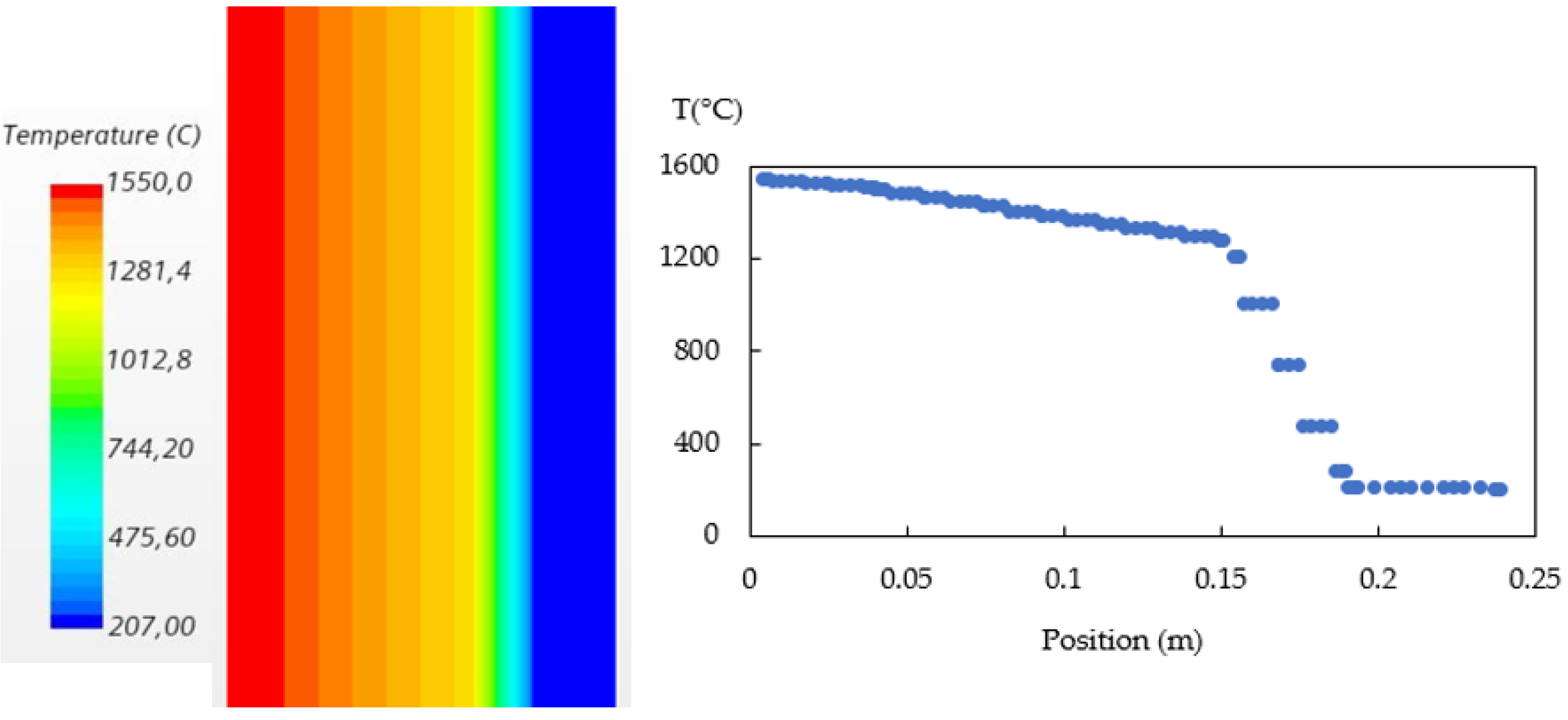
Figure 3 shows the temperature profile of refractory lining as a function of solid layer’s thickness in tundish for a steady-state calculation of C1 described in

Table 4. Taguchi L27 OA, shell temperature (T), heat loss (H_loss), and signal-to-noise (S/N) ratios.

Case	Thermal Conductivity k (W/mK)			Thickness L (m)			T (°C)	Hloss (W)	S/N
	A	B	C	D	E	F
C0	2	2	2	2	2	2	207	3189	-
C1	1	1	1	1	1	1	207	3189	−46.32
C2	1	1	1	1	2	2	168	2485	−44.502
C3	1	1	1	1	3	3	143	2036	−43.105
C4	1	2	2	2	1	1	252	3996	−48.024
C5	1	2	2	2	2	2	205	3157	−46.244
C6	1	2	2	2	3	3	175	2608	−44.849
C7	1	3	3	3	1	1	290	4684	−49.25
C8	1	3	3	3	2	2	238	3749	−47.536
C9	1	3	3	3	3	3	203	3125	−46.17
C10	2	1	2	3	1	2	206	3165	−46.263
C11	2	1	2	3	2	3	174	2587	−44.791
C12	2	1	2	3	3	1	220	3419	−46.849
C13	2	2	3	1	1	2	247	3913	−47.854
C14	2	2	3	1	2	3	208	3213	−46.361
C15	2	2	3	1	3	1	266	4251	−48.498
C16	2	3	1	2	1	2	266	4251	−48.498
C17	2	3	1	2	2	3	153	2220	−43.694
C18	2	3	1	2	3	1	207	3189	−46.319
C19	3	1	3	2	1	3	208	3208	−46.361
C20	3	1	3	2	2	1	262	4173	−48.366
C21	3	1	3	2	3	2	216	3429	−46.689
C22	3	2	1	3	1	3	170	2522	−44.609
C23	3	2	1	3	2	1	207	3189	−46.319
C24	3	2	1	3	3	2	169	2510	−44.558
C25	3	3	2	1	1	3	191	2892	−45.621
C26	3	3	2	1	2	1	256	4073	−48.165
C27	3	3	2	1	3	2	209	3228	−46.403

. The boundary condition of temperature at the hot side is 1550 °C, which is the temperature of molten steel. Temperature decreases gradually in the working layer and permeant layer. In insulation layer, a significant temperature decrease is observed due to low heat conductivity of materials in the region. The calculated temperature at the cold side of shell is 207 °C. A low shell temperature means good heat insulation with less heat loss from the tundish to the surrounding.

Taguchi orthogonal array L27(6 factors and 3 level) was applied to define the design cases and listed in Table 4. The calculated results of shell temperature and heat loss are given in Table 4. C0 is a reference case under normal conditions (A2B2C2D2E2F2). As shown in Table 4, C1 has a normal level of shell temperature 207 °C with heat loss 3189 W. C3 has the lowest shell temperature 143 °C with heat loss 2036 W, while C7 has the highest shell temperature 290 °C with heat loss 4684 W. The corresponding S/N (signal to noise) ratios according to the Taguchi analysis are also listed in Table 4. The temperature at the cold side of shell was used as a design factor. A greater S/N value corresponds to a better heat insulation and less heat loss in the system. From the analysis of the S/N ratio (Figure 4), the levels of the factors to provide the best insulation of the tundish are determined as A1, B1, C1, D3, E3, and F3. Although it is a well-known fact from theory that a thickness increase and a conductivity decrease lead to better heat insulation, the Taguchi analysis can visualize the significant factors. The turning points in signal-to-noise ratios of A and D indicate weak contribution of factor A and D.

As listed in

Table 5. ANOVA table for six factors studied (response: shell temperature).

Factor	DOF	Adj SS	Contribution	Adj MS	F-Value
A	2	283.1	0.76%	141.5	0.55
B	2	2468.5	6.61%	1234.2	4.84
C	2	11,242.3	30.13%	5621.2	22.03
D	2	266.7	0.71%	133.3	0.52
E	2	3095.6	8.30%	1547.8	6.06
F	2	16,388.7	43.92%	8194.4	32.11
Error	14	3572.8	9.57%	255.2
Total	26	37,317.7	100%

, the term DOF represents the degree of freedom. The adjusted sums of squares (Adj SS) indicate the relative importance of each factor. Adjusted mean squares (Adj MS) measure how much variation a term explains. The factor with the biggest coefficient and biggest adjusted sum of squares has the greatest impact. As suggested in Table 5, it indicates that the contribution order to decrease the heat loss in the tundish process is factor F > C > E > B > A > D, according to ANNOV analysis in Table 5. The factor F and C (heat conductivity and thickness of insulation layer) had the highest contribution on the heat loss in tundish, which is consistent with the results from Taguchi method (Figure 4). In the cases of insulation layer with greater thicknesses, the steel bath energy losses decrease due to the stronger thermal barrier induced by the lower thermal conductivity material.

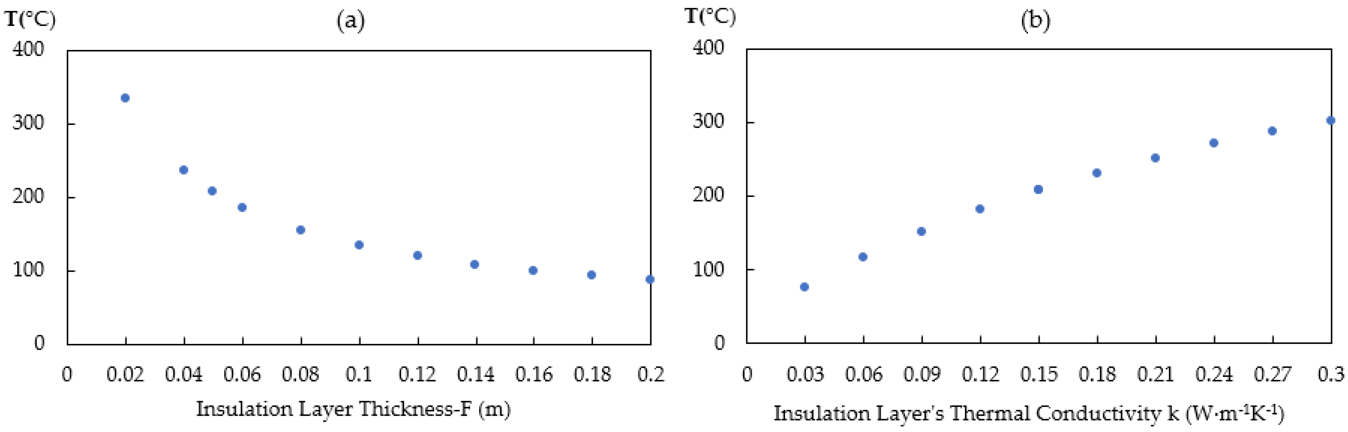
Figure 5a shows the predicted shell temperature corresponding to the insulation layer thickness. Increasing the thickness of the insulation layer from 0.02 to 0.2 m lowers the shell temperatures from 335 to 87 °C. The result indicates insulation layer is an effective thermal barrier, thus lowering the shell temperature. The gains of the insulation layer thickness over 0.1 m are less significant but greater thicknesses leads to higher investment costs. Figure 5b highlights the predicted shell temperature corresponding to the thermal conductivities of the insulation layer materials. It can be observed that increasing the thermal conductivity from 0.03 to 0.3 raises the shell temperature from 77 to 302 °C. Moreover, a nearly linear relationship is found between shell temperature and material’s thermal conductivity.

3.2. Two-Dimensional Transient Heat Transfer (Tundish Preheating)

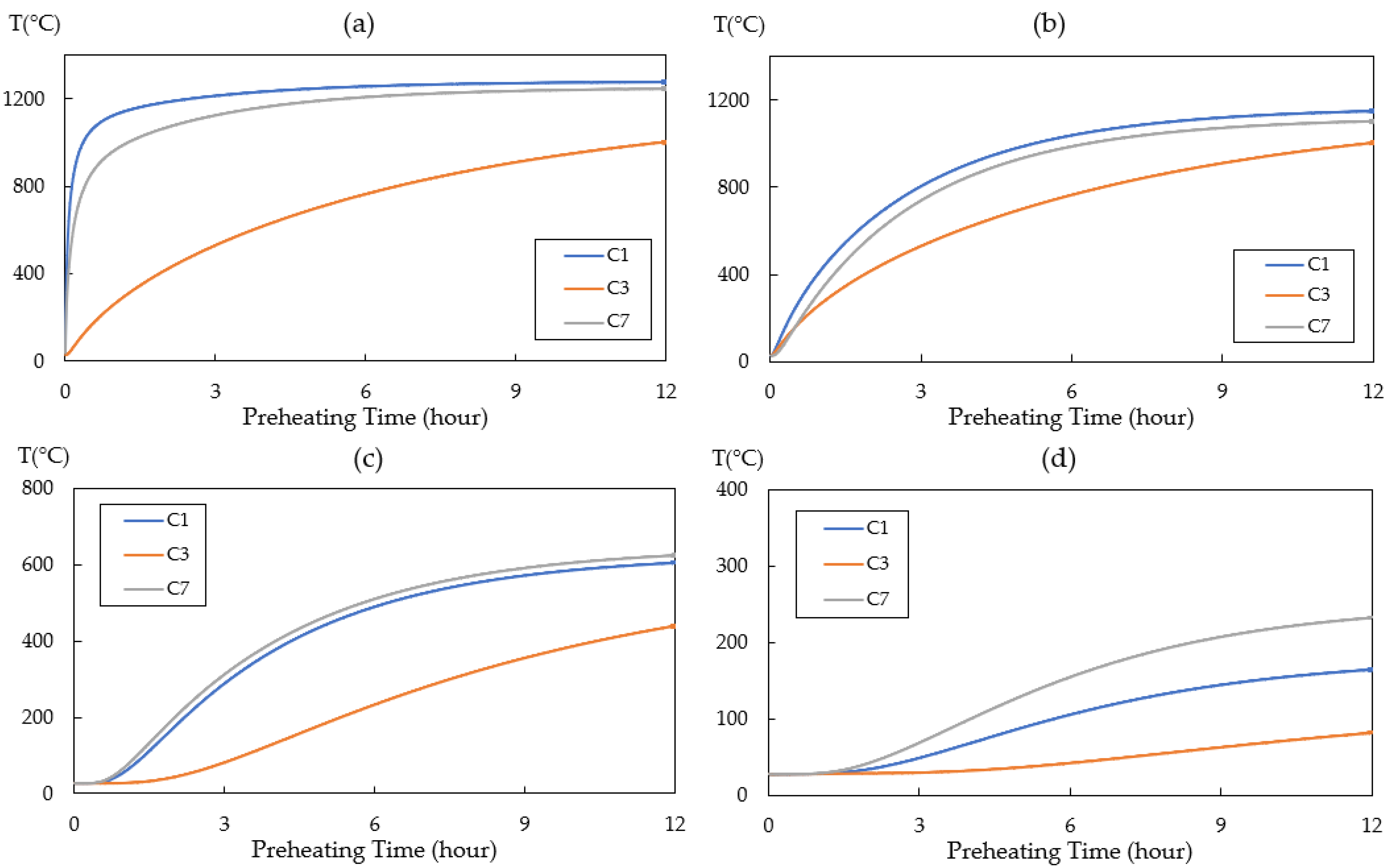
Figure 6 shows that the average temperature of refractory lining during the preheating of the tundish. Three different cases (C1, C3, and C7) were selected based on Table 4 to represent the normal, low, and high heat loss conditions, respectively. The initial temperature was set to 27 °C and the hot surface temperature was set to 1300 °C as the tundish preheating temperature. C1 and C7 have quite similar thermal behavior in the working lining (Figure 6a) and permeant lining (Figure 6b). C3 (A1B1C1D1E3F3) shows the lowest predicted temperature on the shell due to low heat conductivity of refractory lining, thick permanent and insulation layer. To consider energy cost and heat efficiency for a normal heat loss case C1, the increase rate of average temperature in the permanent layer (Figure 5b) is about 4.3 °C/min in the first three hours and 0.65 °C/min in the next nine hours. This means the heating efficiency decrease significantly after the first three hours. Therefore, it is necessary to consider the fuel cost and burner efficiency in order to calculate the economic thickness of insulation.

3.3. Three-Dimensional Steady-State Conjugate Heat Transfer

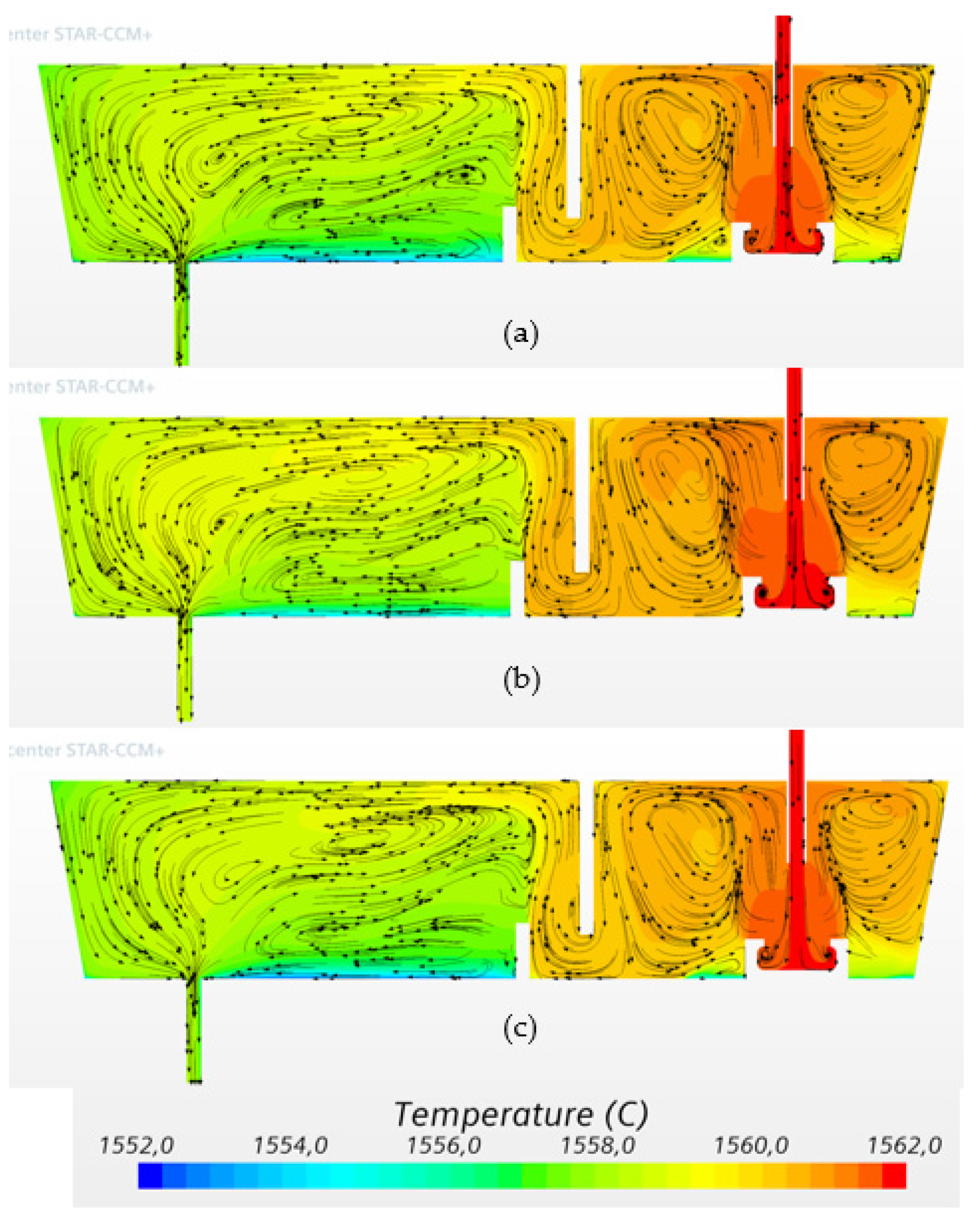
Figure 7 shows the predicted flow pattern and temperature distributions on the symmetry plane after pouring molten steel from ladle. The flow patterns in the entry zone have similar characteristics for the three cases. For the tundish equipped with a turbulence inhibitor, the entering flow reoriented towards the top surface and formed two circulation loops at the symmetry plane of the inlet chamber. The high velocity in the inlet chamber leads to a strong mixing. The high temperature zone caused by the incoming stream is confined within the region near the inlet owing to the presence of the weir. The low temperature region is found at the tundish bottom around the turbulence inhibitor due to the formation of dead zone. The flow moves underneath the weir and downstream towards the outlet chamber controlled by the dam. In the outlet chamber, a big counterclockwise-circulation loop is observed. The lowest temperature is located near the bottom between the weir and the outlet because of low fluid movement within dead zone. The flow patterns in outlet chamber show slightly different for the three studied cases.

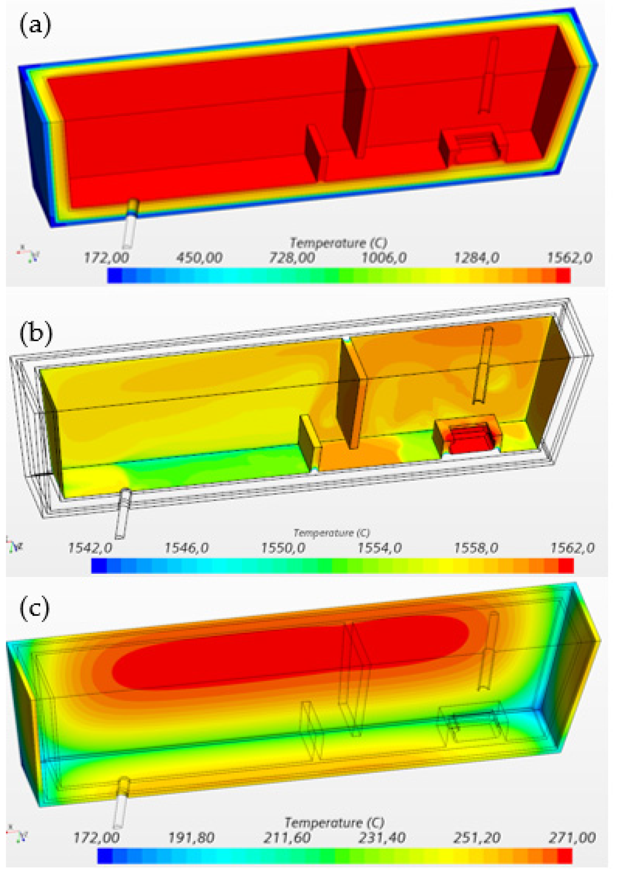
Figure 8a shows the 3D temperature distribution in the four solid layers of the tundish (working lining, permanent lining, insulation lining, and steel shell). The calculation was run at steady state. Temperature gradient in the solid layers is obvious due to the difference in heat conductivity in material. Figure 8b shows the temperature distribution in the working lining. In the turbulence inhibitor, the highest temperature is observed due to high temperature of the incoming molten steel. Two low temperature regions are observed. One occurs at the bottom of inlet chamber close to the turbulence inhibitor, while the other appears at the tundish bottom between the dam and outlet. This is mainly due to the lower flow velocity reducing the convective heat transfer in these regions. When the molten steel flows through the entire tundish, the hotter molten steel heats the refractory inner layer-working lining. Therefore, the temperature profile of the working lining can reflect the temperature of the molten steel in the tundish. Figure 8c displays the temperature distribution of refractory outer layer steel shell. The lowest temperature is 172 °C and the highest temperature is 271 °C. The low temperature region locates at the interface of the tundish walls and the high temperature region locates at the center of the tundish front/back walls.

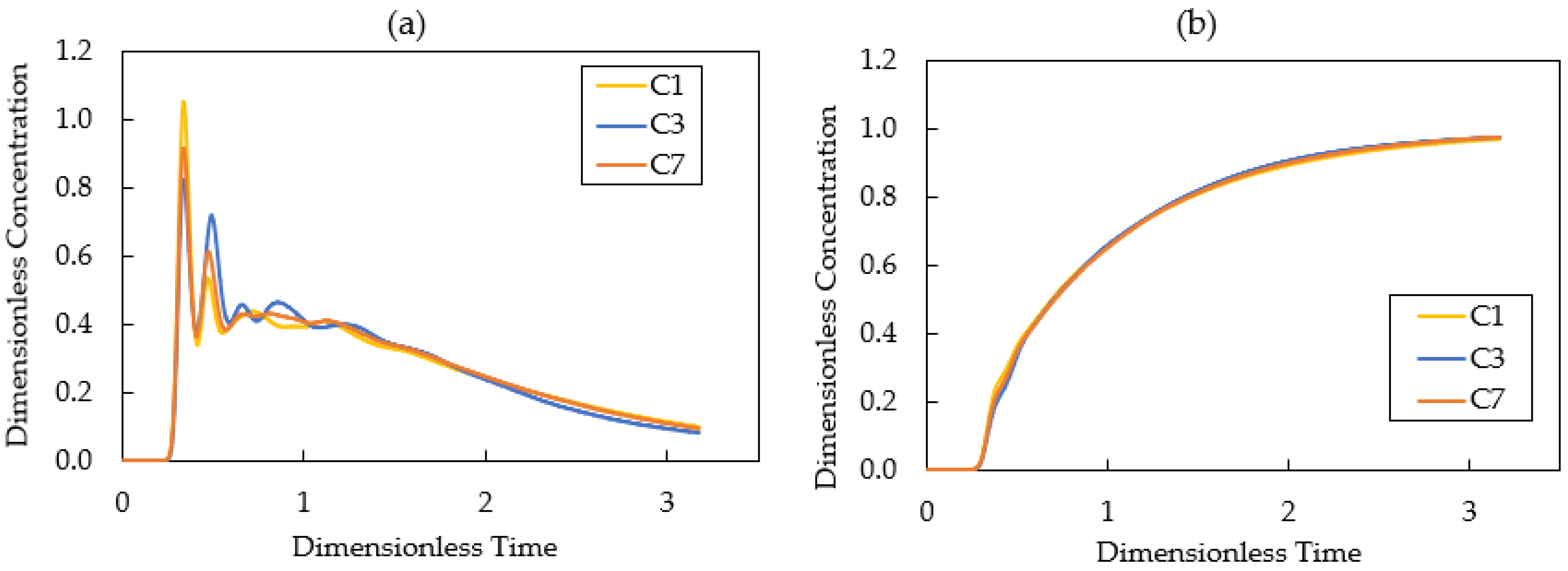
Figure 9 and

Table 6. Analysis of residence time distribution for the tundish configurations: C1, C3, and C7.

Case	ttheoretical (s)	tmean (s)	tmin (s)	tmax (s)	t0.2 (s)	t0.8 (s)	tmix (s)	Vd/V (%)	Vp/V (%)	Vm/V (%)
C1	820	729	201	271	293	1194	901	11	25	64
C3	820	729	204	271	316	1175	859	11	25	64
C7	820	737	201	271	303	1193	890	10	25	65

display the calculated E-curve, F-curve, and RTD analysis for the selected three cases, case C1, C3, and C7, respectively. In Figure 9a, the E-curve of three cases shows very similar shape. They have same peak value time at 271 s. The difference in dead volume fraction is within 1%. The theoretical residence time for three cases are 820 s. The predicted mean resident time for C1, C3, and C7 are 729 s, 729 s, and 737 s, respectively. Figure 9b shows the CFD modeling results of the F-curves of the three studied tundish configurations: C1, C3, and C7. The three F-curves are very close to each other. The model assumes that an intermixing zone exists between the value 0.2 and 0.8 of the dimensionless concentration of the tracer. The predicted intermixing time for C1, C3, and C7 is 901 s, 859 s, and 890 s, respectively. C3, the tundish with lowest heat loss, owns the shortest intermixing time. From the results mentioned above, it shows that the selected configurations of the tundish refractory lining have little difference in thermal hydraulic behavior of molten steel in tundish under steady-state condition. The main reasons are: (i) even for the highest heat loss case (C7), the thickness of insulation layer is 0.0375m, which can provide effective heat insulation for the tundish as shown in Figure 5a; (ii) the heat loss through refractory lining is much lower (18%) compared to the heat loss through top surface (82%). These value were calculated from the CFD results by the integration of the heat flow at the boundaries. The heat loss through walls and top surface is 40 kW and 187 kW, respectively.

3.4. Three-Dimensional Transient Conjugate Heat Transfer

The initial conditions of the temperature in the refractory lining were based on the results of 2D transient tundish preheating cases in Section 3.2. A normal preheating time, 3 h, was applied for the calculation. The average temperature was used in four solid layers, as listed in

Table 7. Initial conditions of temperature (°C) for the transient conjugate heat transfer analysis (3 h preheating).

Case	Working Lining	Permanent Lining	Insulation Lining	Steel Shell	Molten Steel
C3 preheating	1203	529	81	30	1562
C7 preheating	1125	738	312	69	1562
C3 without preheating	30	30	30	30	1562

. It is clear to see the large difference between the temperature of refractory linings and the steel temperature even when the tundish is preheated for 3 h, which lead to an unsteady state heat during the tundish casting operation.

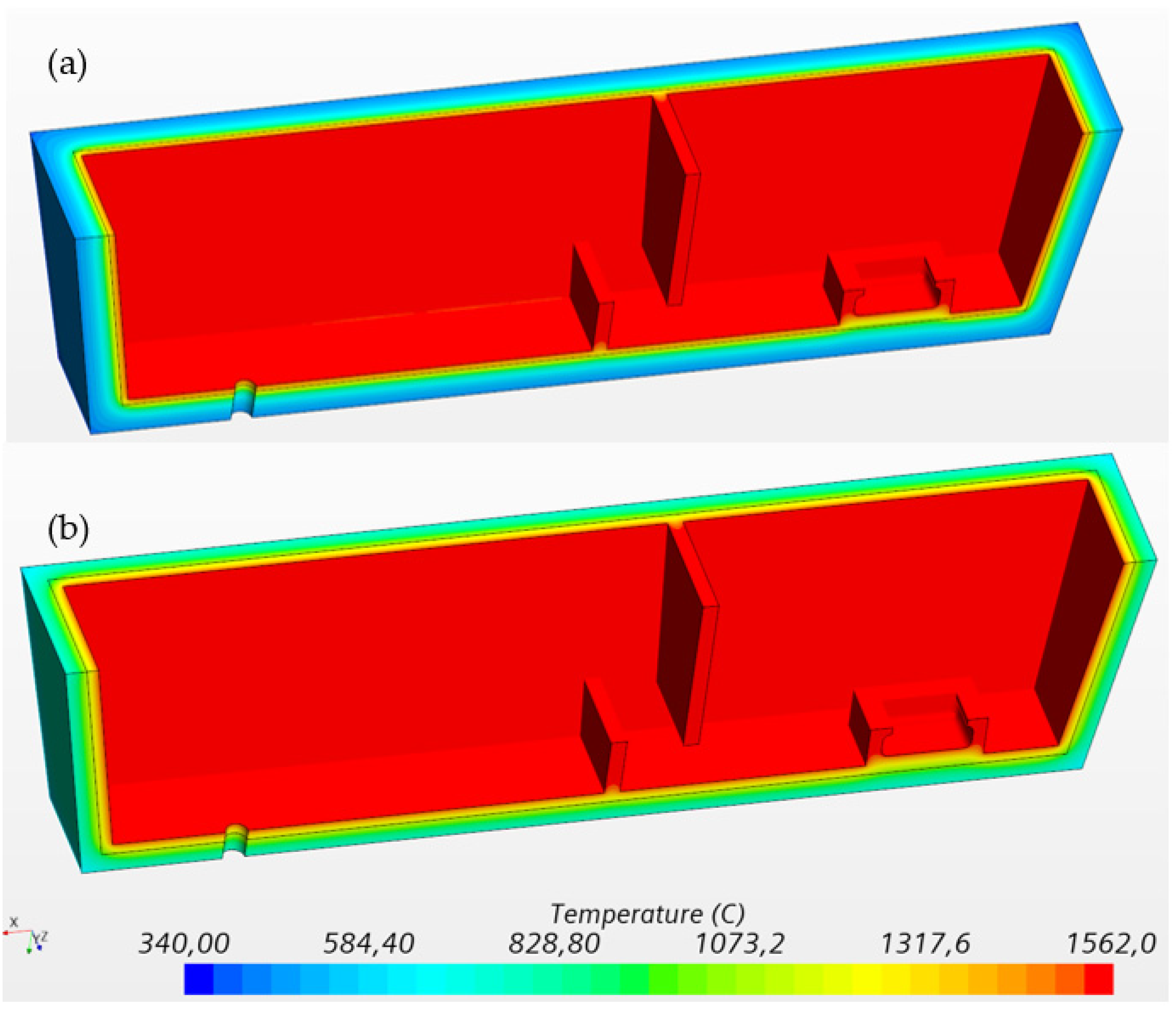
Figure 10 shows the 3D temperature distribution in the two refractory layers of the tundish (inner-working lining, and outer-permanent lining) for the C3 and C7 (3 h preheating) after 1 h casting operation. The liquid level keeps constant for the simplification. It is clear that temperature C3 has a lower temperature in the permanent lining compared to that of C7. This is due to the higher heat insulation and thicker permanent lining from C3.

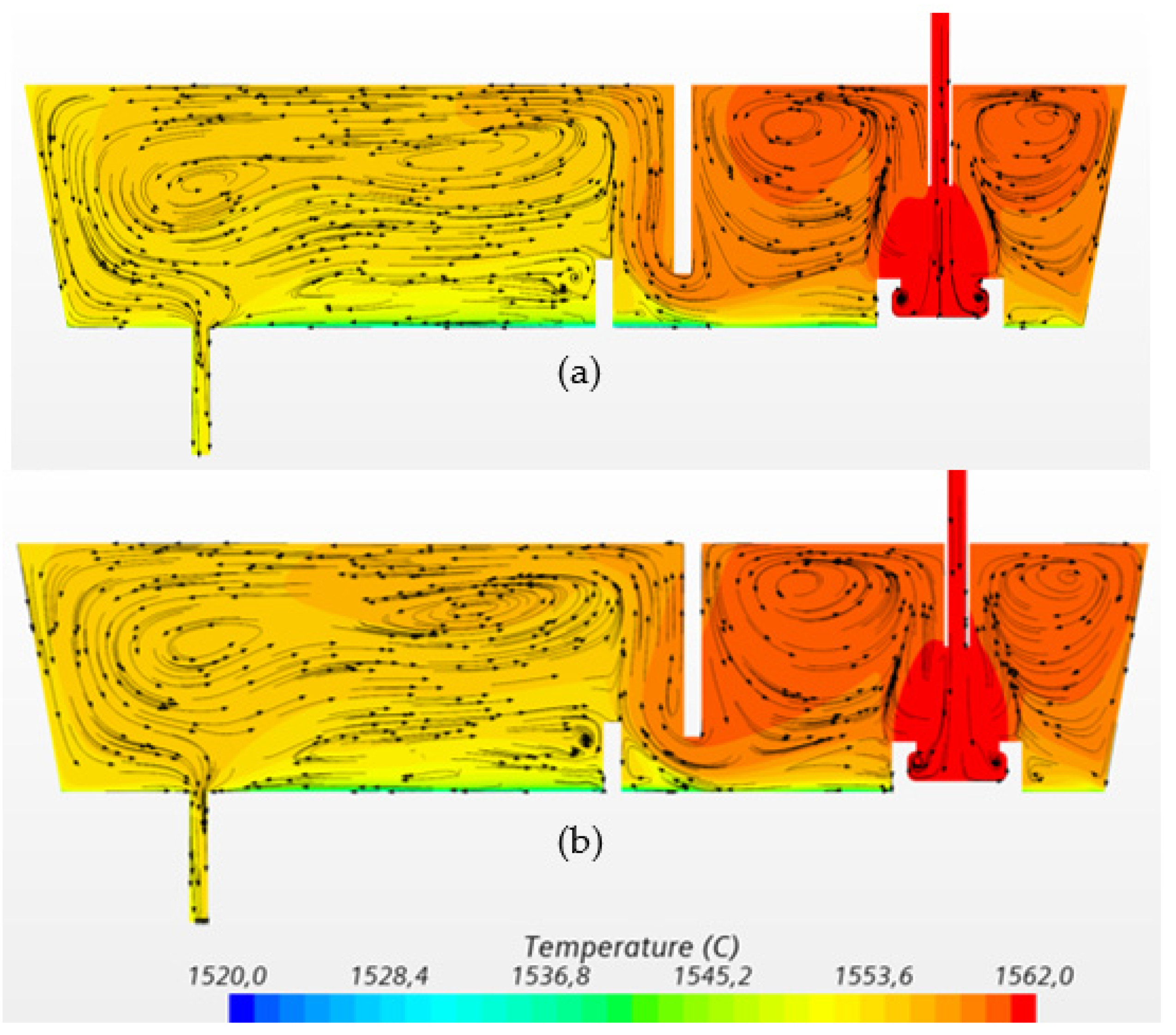
The calculated transient flow pattern and temperature distributions of molten steel on the symmetry plane for C3 (with preheating) and C7 (with preheating) after 1 h casting are shown in Figure 11. The main flow patterns of C3 and C7 are quite similar. A slightly higher temperature of molten steel can be observed in Figure 11b compared to Figure 11a in inlet chamber. In addition, the temperature in the inlet chamber is higher than the outlet chamber. The low temperature region locates at the bottom of the tundish between the inlet and outlet.

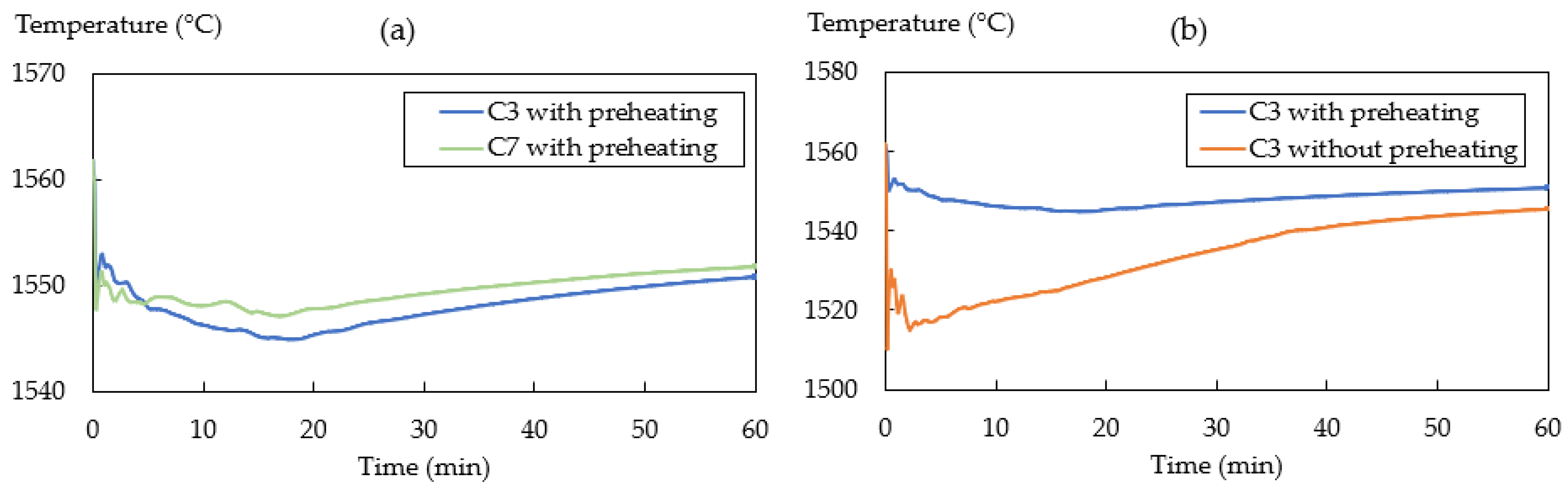
The calculated average temperatures at the tundish outlet for C3 (with preheating) and C7 (with 3 h preheating) during 1 h casting are shown in Figure 12a. Due to temperature difference between molten steel and refractory, a large portion of heat flows through the refractory lining, leading to the temperature drop at the outlet in the first 15 to 20 min for C3 and C7. After that, the outlet temperature increases gradually. It is interesting to note that the outlet temperature of C7 is slightly higher than C3, though C3′s configuration has a better thermal insulation. At the time of 60 min, the outlet temperature for case C3 and case C7 is 1550.7 °C and 1551.7 °C, respectively, which is around 10 °C lower than the inlet temperature.

To study the effect of tundish preheating, the calculated outlet temperatures for two cases (C3 with and without preheating) during the 1 h casting are shown in Figure 12b. A significant temperature drop is observed in the first few minutes, which means that a large amount of heat flows to the refractory lining. At the time of 60 min, the outlet temperature for C3 with preheating and without preheating is 1550.7 °C and 1545.5 °C, respectively.

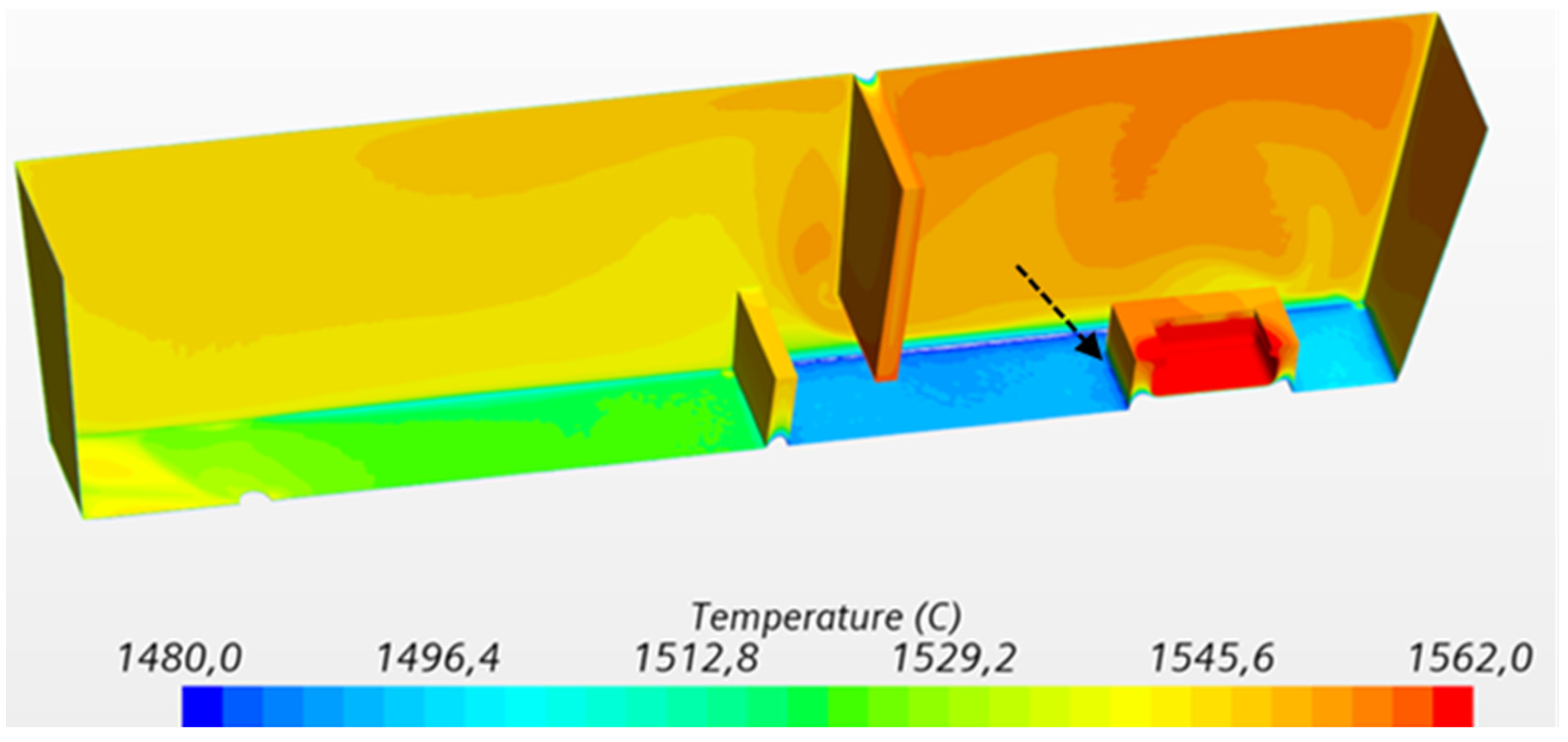
Figure 13 gives the temperature distribution in the working lining after 1 h casting for C3 without preheating. At the bottom of inlet chamber, there is a region with very low temperature. When the tundish was equipped with a turbulence inhibitor, the entering flow reoriented towards the top surface. This leads to a low velocity region at the bottom of the inlet chamber. Due to the less convective heat transfer in this region and the larger heat loss through refractory, the low temperature region is formed. In addition, the thermal buoyancy has also an impact on the temperature distribution, causing a lower temperature region close to the bottom. However, the temperature inside the turbulence inhibitor is very high, close to the inlet temperature. As marked by arrow in Figure 13, the temperature gradients and thermal shocks around the turbulence inhibitor can lead to high thermal stress, resulting in cracking or shattering of the turbulence inhibitor. Compared to the steady-state result in Figure 8b, the transient calculation shows a higher temperature gradient.

Tapping molten steel into a tundish without preheating is always undesirable. It adversely affects the refractory lining. Moreover, it causes a significant temperature drop of the molten steel. Hence, tundish preheating is very crucial for proper control of superheat of molten steel.

4. Conclusions

A simulation-based digital design methodology that combined CFD simulation and Taguchi analysis was presented to study conjugate heat transfer in a single-strand tundish. The objective is to analyze the effects of thickness and thermal conductivity of refractory lining on the thermal states of a tundish. Six factors were selected, namely, thermal conductivity of working lining (A), permanent lining (B), insulation lining (C) and thickness of working lining (D), permanent lining (E), and insulation lining (F). The main conclusions of this study can be drawn as below:

• From the results of 2D steady-state heat transfer, the contribution of studied six factors in a greater heat loss in tundish is F > C > E > B > A > D. The insulation lining’s thickness and thermal conductivity had the greatest influence on heat loss in tundish.
• The heat gains of the insulation layer thickness over 0.01 m are less significant. Decreasing the thermal conductivity of the insulation layer material leads to a decrease in heat loss with a nearly linear relationship.
• From the analysis of tundish preheating, case C3 (A1B1C1D1E3F3) shows the lowest predicted temperature due to the best heat insulation in comparison with C1 (A1B1C1D1E1F1) and C7(A1B3C3D3E1F1).
• The selected configuration (case C1, C3, and C7) of refractory lining has a minor effect on the thermal hydraulic behavior of molten steel in the tundish under the steady state condition. In case C3, the heat loss through refractory lining is much lower (18%) compared to the heat loss through top surface (82%).
• From the transient conjugate heat transfer calculation of case C3 and C7 with preheating, it shows that a large portion of heat flows through the refractory lining, resulting in a temperature drop in the first 15 to 20 min.
• For case C3 without preheating, a large temperature gradient is observed near the turbulence inhibitor. There is a risk of cracking or shattering of turbulence inhibitor if tapping molten steel into a tundish without preheating.

For the future work, it is important to analyze the thermal insulation with respect to cost. An increased thickness of lining can be more expensive than the cost saving from recovered heat of a thermal optimum lining design. That is to say, it is necessary to consider fuel consumption and burner efficiency during tundish preheating in order to obtain the economic optimum thickness of insulation. During the casting operation, large amounts of heat can be lost due to radiation from the top surface of the melt. The effect of slag on the thermal states of the tundish needs also be considered. In addition, an advanced optimization algorithm is needed to improve the design process. A faster computer will enable sensitivity analysis for large parameter sets aiming at true optimization to be performed, rather than the limited number of cases.

To sum up, the present study demonstrated that a simulation-based digital design methodology, combined CFD modelling and Taguchi analysis, was effective in finding a better tundish design. This improves the tundish performance by realizing time and cost conservation. The results for process optimization continue to encourage the application of the simulation-based digital design methodology in research field and industrial practice.

References

- Szekely, J.; Ilegbusi, O.J. The Physical and Mathematical Modeling of Tundish Operations; Springer Science and Business Media LLC: New York, NY, USA, 1989. [Google Scholar]
- Mazumdar, D.; Guthrie, R.I.L. The Physical and Mathematical Modelling of Continuous Casting Tundish System. ISIJ Int. 1999, 39, 524–547. [Google Scholar] [CrossRef]
- Chattopadhyay, K.; Isac, M.; Guthrie, R.I.L. Physical and Mathematical Modelling of Steelmaking Tundish Operations: A Review of the Last Decade (1999–2009). ISIJ Int. 2010, 50, 331–348. [Google Scholar] [CrossRef] [Green Version]
- Kemeny, F.; Harris, D.J.; McLean, A.; Meadowcroft, T.R.; Young, D.J. Fluid flow studies in the tundish of a slab caster. In Proceedings of the 2nd Process Technol Conference on Continuous Casting of Steel, Chicago, IL, USA, 23–25 February 1981; pp. 232–245. [Google Scholar]
- Sahai, Y.; Emi, T. Tundish Technology for Clean Steel Production; World Scientific Publishing Co.: Singapore, 2008. [Google Scholar]
- Zhang, J.H.; Chen, Y.X.; Yang, D.Z. Process design and life anylysis of tundish lining. Metalurgija 2021, 60, 191–194. [Google Scholar]
- Kato, Y. Refractories for Continuous Casting; Nippon Steel Technical Report No. 125; Nippon Steel Corporation: Tokyo, Japan, 2020. [Google Scholar]
- Neves, L.; Tavares, R.P. Analysis of the mathematical model of the gas bubbling curtain injection on the bottom and the walls of a continuous casting tundish. Ironmak. Steelmak. 2017, 44, 559–567. [Google Scholar] [CrossRef]
- Aguilar-Rodriguez, C.E.; Ramos-Banderas, J.A.; Torres-Alonso, E.; Solorio-Diaz, G.; Hernández-Bocanegra, C.A. Flow characterization and inclusions removal in a slab tundish equipped with bottom argon gas feeding. Metallurgist 2018, 61, 1055–1066. [Google Scholar] [CrossRef]
- Yang, B.; Lei, H.; Zhao, Y.; Xing, G.; Zhang, H. Quasi-symmetric transfer behavior in an asymmetric two-strand tundish with different turbulence inhibitor. Metals 2019, 9, 855. [Google Scholar] [CrossRef] [Green Version]
- Neumann, S.; Asad, A.; Schwarze, R. Numerical simulation of an industrial-scale prototypical steel melt tundish considering flow control and cleaning strategies. Adv. Eng. Mater. 2020, 22, 1900658. [Google Scholar] [CrossRef] [Green Version]
- Tkadlečková, M.; Walek, J.; Michalek, K.; Huczala, T. Numerical Analysis of RTD Curves and Inclusions Removal in a Multi-Strand Asymmetric Tundish with Different Configuration of Impact Pad. Metals 2020, 10, 849. [Google Scholar] [CrossRef]
- Wang, Q.; Zhang, C.-J.; Li, R. CFD investigation of effect of multi-hole ceramic filter on inclusion removal in a two-strand tundish. Metall. Mater. Trans. B 2020, 51, 276–292. [Google Scholar] [CrossRef]
- Silva, H.; Silva, C.; Alves Da Silva, I.; Barros, A. Study of Flow Modification and Inclusion Removal in Slag Tundish due to Bottom Gas Injection. Tecnol. Metal. Mater. Miner. 2018, 15, 167–174. [Google Scholar] [CrossRef]
- Qin, X.; Cheng, C.-G.; Li, Y.; Zhang, C.; Zhang, J.; Yan, J. A Simulation Study on the Flow Behavior of Liquid Steel in Tundish with Annular Argon Blowing in the Upper Nozzle. Metallurigst 2019, 9, 225. [Google Scholar] [CrossRef] [Green Version]
- Chatterjee, S.; Chattopadhyay, K. Transient steel quality under non-isothermal conditions in a multi-strand billet caster tundish: Part II. Effect of a flow-control device. Ironmak. Steelmak. 2017, 44, 413–420. [Google Scholar] [CrossRef]
- Yue, Q.; Zhang, C.B.; Pei, X.H. Magnetohydrodynamic flows and heat transfer in a twin-channel induction heating tundish. Ironmak. Steelmak. 2017, 44, 227–236. [Google Scholar] [CrossRef]
- Tang, H.; Liu, J.; Wang, K.; Xiao, H.; Li, A.; Zhang, J. Progress and Perspective of Functioned Continuous Casting Tundish Through Heating and Temperature Control. Acta Metall. Sin. 2021, 57, 1229–1245. [Google Scholar] [CrossRef]
- Sheng, D.-Y.; Jönsson, P.G. Effect of thermal buoyancy on fluid flow and residence-time distribution in a single-strand tundish. Materials 2021, 14, 1906. [Google Scholar] [CrossRef] [PubMed]
- Sheng, D.-Y.; Zou, Z. Application of tanks-in-series model to characterize non-ideal flow regimes in continuous casting tundish. Metals 2021, 11, 208. [Google Scholar] [CrossRef]
- Sheng, D.Y.; Yue, Q. Modeling of Fluid Flow and Residence-Time Distribution in a Five-strand Tundish. Metals 2020, 10, 1084. [Google Scholar] [CrossRef]
- Sheng, D.-Y.; Chen, D. Comparison of Fluid Flow and Temperature Distribution in a Single-Strand Tundish with Different Flow Control Devices. Metals 2021, 11, 796. [Google Scholar] [CrossRef]
- Sheng, D.Y. Mathematical Modelling of Multiphase Flow and Inclusion Behavior in a Single-Strand Tundish. Metals 2020, 10, 1213. [Google Scholar] [CrossRef]
- Sheng, D.-Y. Synthesis of a CFD Benchmark Exercise: Examining Fluid Flow and Residence-Time Distribution in a Water Model of Tundish. Materials 2021, 14, 5453. [Google Scholar] [CrossRef] [PubMed]
- Sheng, D.-Y. Design optimization of a single-strand tundish based on cfd-taguchi-grey relational analysis combined method. Metals 2020, 10, 1539. [Google Scholar] [CrossRef]
- Incropera, F.P.; DeWitt, D.P.; Bergmann, T.L.; Lavine, A.S. Fundamentals of Heat and Mass Transfer, 6th ed.; John Wiley & Sons Inc.: New York, NY, USA, 2006. [Google Scholar]
- Minitab 18 Statistical Software; Minitab, Inc.: State College, PA, USA, 2017; Available online: www.minitab.com (accessed on 7 June 2017).
- Taguchi, G.; Chowdhury, S.; Wu, Y. Taguchi’s Quality Engineering Handbook; John Wiley & Sons Inc.: Hoboken, NJ, USA, 2005. [Google Scholar]
- Taguchi, G. Off-line and On-line Quality Control Systems. In Proceedings of the International Conference on Quality Control, Tokyo, Japan, 17–20 October 1978. [Google Scholar]
- Fisher, R.A. Statistical Methods for Research Workers; Oliver & Boyd: Edinburgh, UK, 1925. [Google Scholar]
- Siemens, P.L.M. STAR-CCM + User Guide Version 15.04; Siemens PLM Software Inc.: Munich, Germany, 2019. [Google Scholar]
- Patankar, S.V. Numerical Heat Transfer and Fluid Flow; Hemisphere Publishing Corporation: New York, NY, USA, 1980. [Google Scholar]
- Shih, T.H.; Liou, W.W.; Shabbir, A.; Yang, Z.; Zhu, J. A New k-ε eddy viscosity model for high reynolds number turbulent flows-model development and validation. Comput. Fluids 1994, 24, 227–238. [Google Scholar] [CrossRef]
- Spalding, D.B. A note on mean residence-times in steady flows of arbitrary complexity. Chem. Eng. Sci. 1958, 9, 74–77. [Google Scholar] [CrossRef]
- Jha, P.K.; Dash, S.K. Effect of outlet positions and various turbulence models on mixing in a single and multi-strand tundish. Int. J. Numer. Methods Heat Fluid Flow 2002, 12, 560–584. [Google Scholar] [CrossRef]
Figure 1.
Schematic diagram and a thermal network model of tundish refractory lining.
Figure 2.
Dimensions of a single-strand tundish with flow control devices (dam, weir, and turbulence inhibitor), unit: mm, (a) main view; (b) side view; (c) zoomed top view of turbulence inhibitor.
Figure 3.
Calculated temperature profile in refractory lining (case C1).
Figure 4.
Mean S/N ratio (shell temperature) for each factor at levels 1–3.
Figure 5.
Predicted shell temperature corresponding to (a) insulation layer thickness and (b) insulation material’s thermal conductivity.
Figure 6.
Average temperature of refractory lining in (a) working lining (b) permanent lining (c) insulation lining (d) steel shell during tundish preheating for 12 h under normal (C1), low (C3), and high (C7) heat loss conditions.
Figure 7.
Calculated temperature and flow pattern on the symmetry plane of the tundish under condition of: (a) normal (C1), (b) low (C3), and (c) high (C7) heat loss.
Figure 8.
Calculated temperature distribution in the tundish (a) all solid layers; (b) working lining; (c) steel shell.
Figure 9.
(a) E-curve and (b) F-curve for the tundish configurations: C1, C3, and C7.
Figure 10.
Calculated temperature distribution in working and permeant lining of the tundish after 1 h casting: (a)—case C3 (with preheating); (b)—case C7 (with preheating).
Figure 11.
Calculated temperature distribution of molten steel on the symmetry plane of the tundish after 1 h casting: (a) C3 (with preheating); (b) C7 (with preheating).
Figure 12.
Transient result of the average temperature at the outlet of the tundish after 1 h casting for: (a) C3 and C7 with preheating; (b) C3 with and without preheating.
Figure 13.
Calculated temperature profile in the working lining after 1 h casting for case C3 without preheating.