
Advanced Image Analysis Methods for Automated Segmentation of Subnuclear Chromatin Domains
 , , , , and
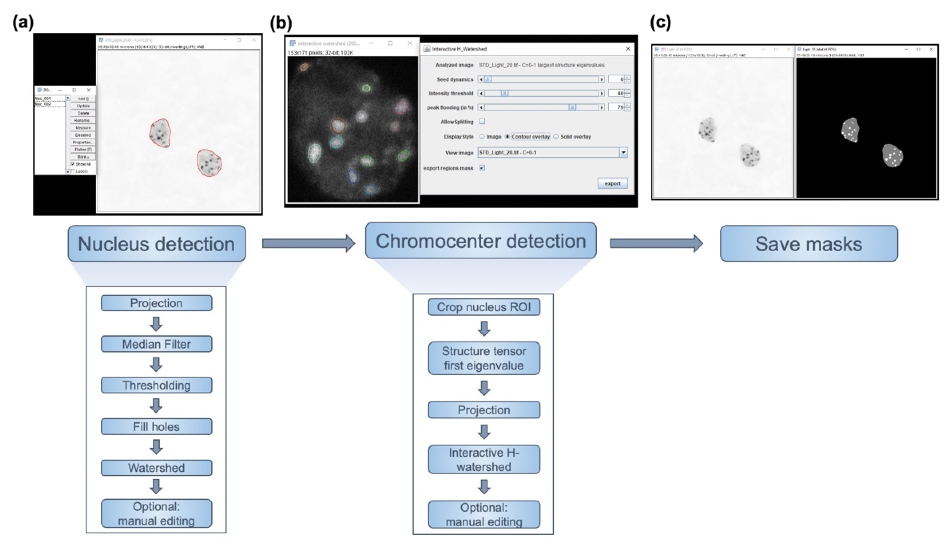
Abstract
:1. Introduction
2. Results and Discussion
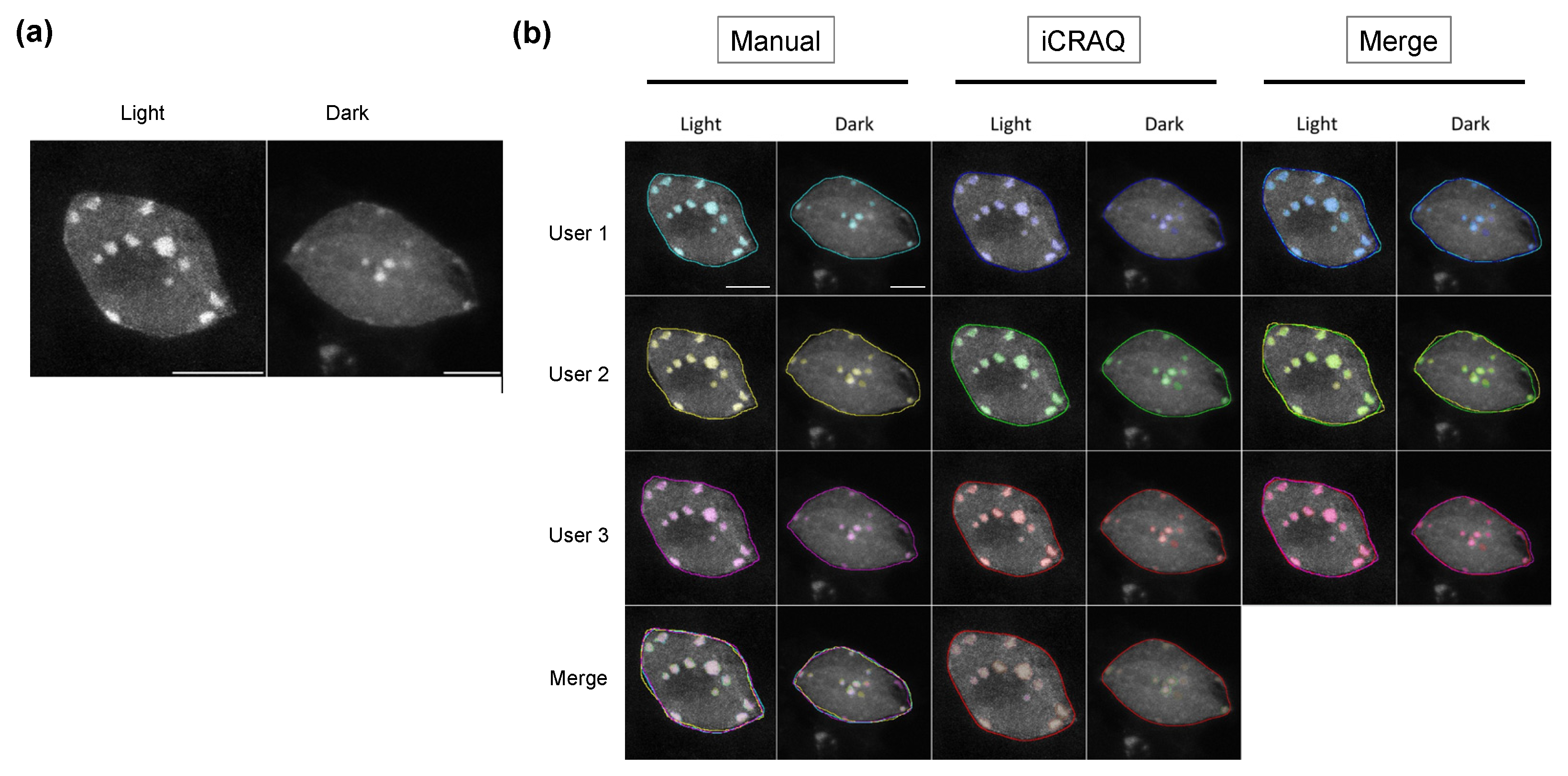
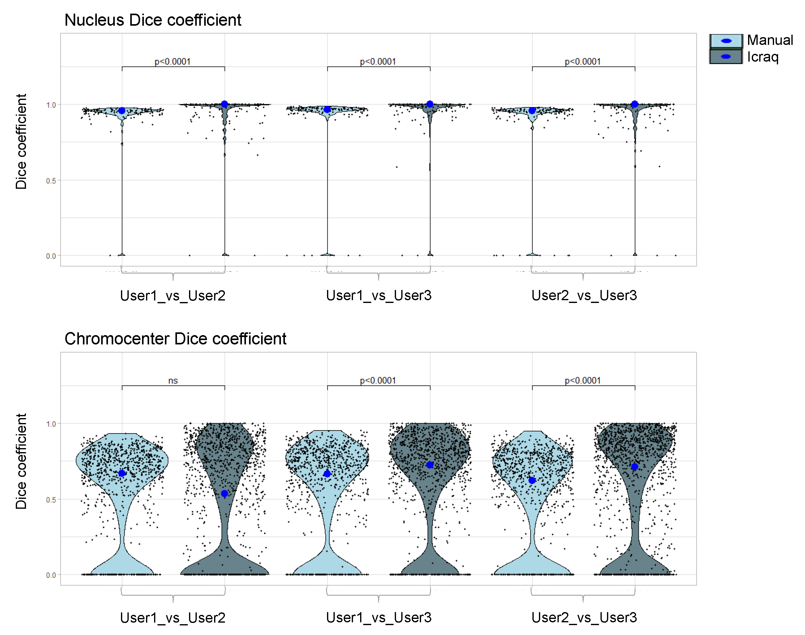
2.1. iCRAQ: A Plug-In Assisted Tool for Segmentation of Nucleus and Chromocenters
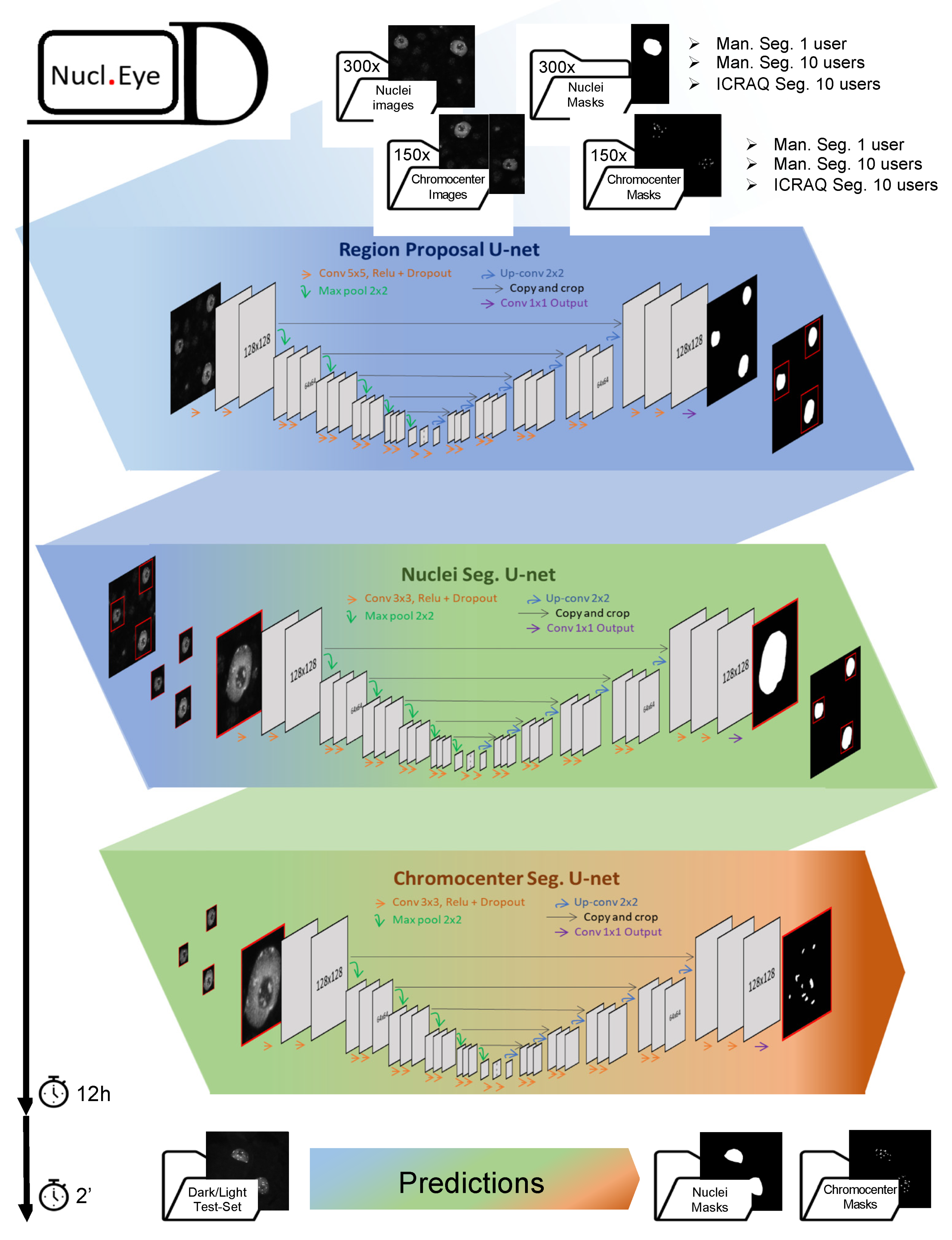
2.2. Nucl.Eye.D: A Fully Automated Deep Learning Pipeline for Segmentation of Nucleus and Subnuclear Structures
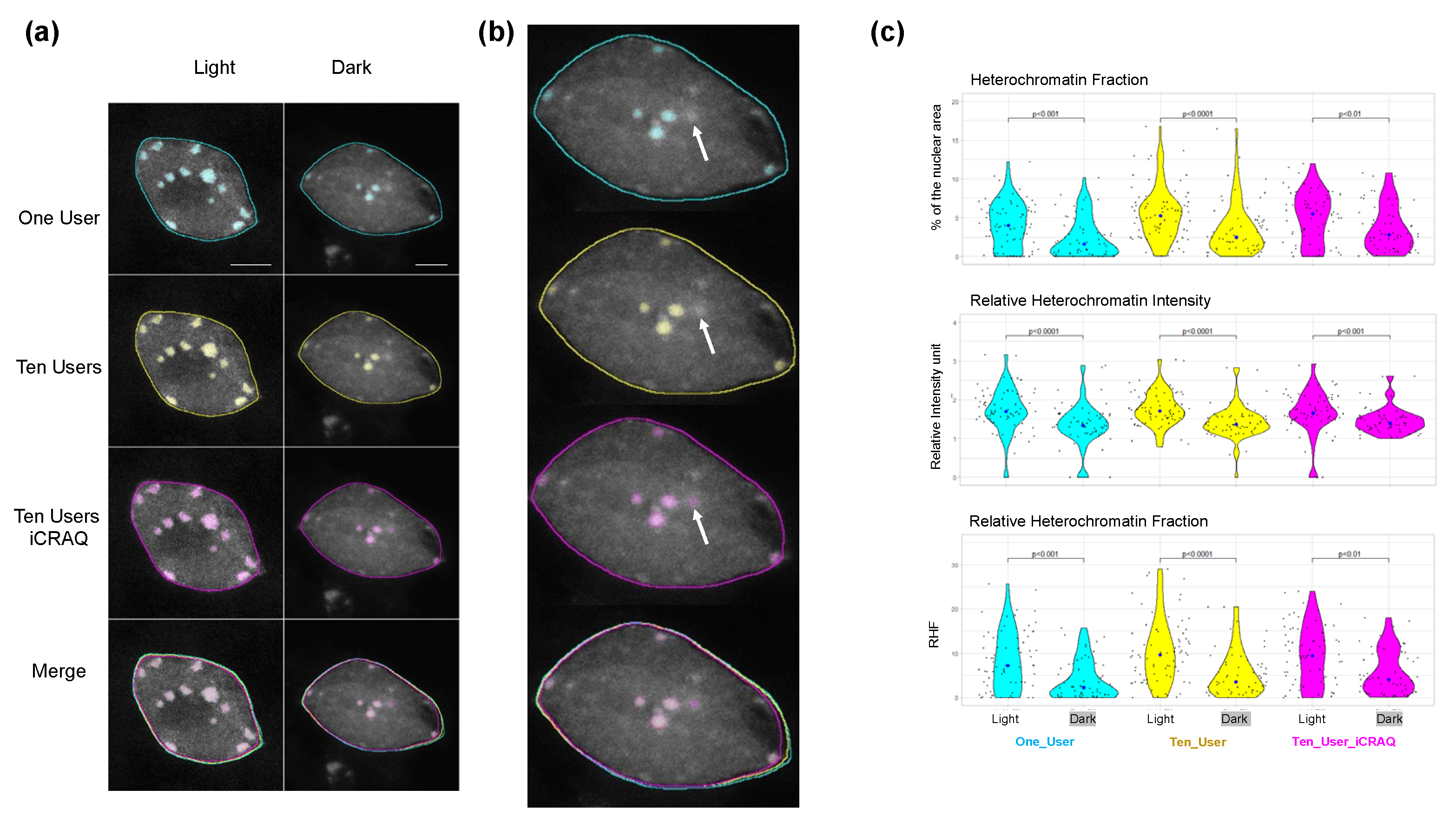
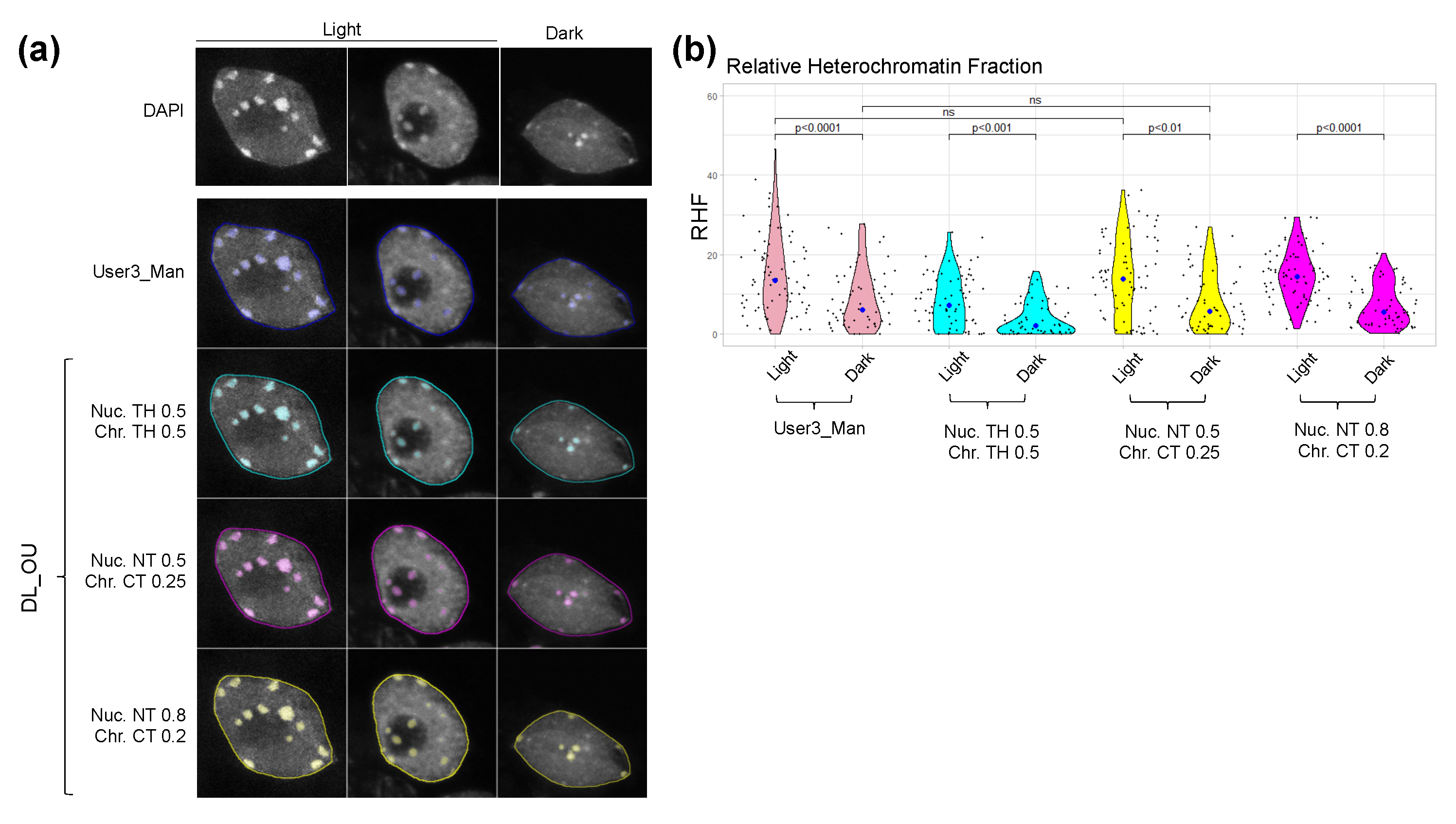
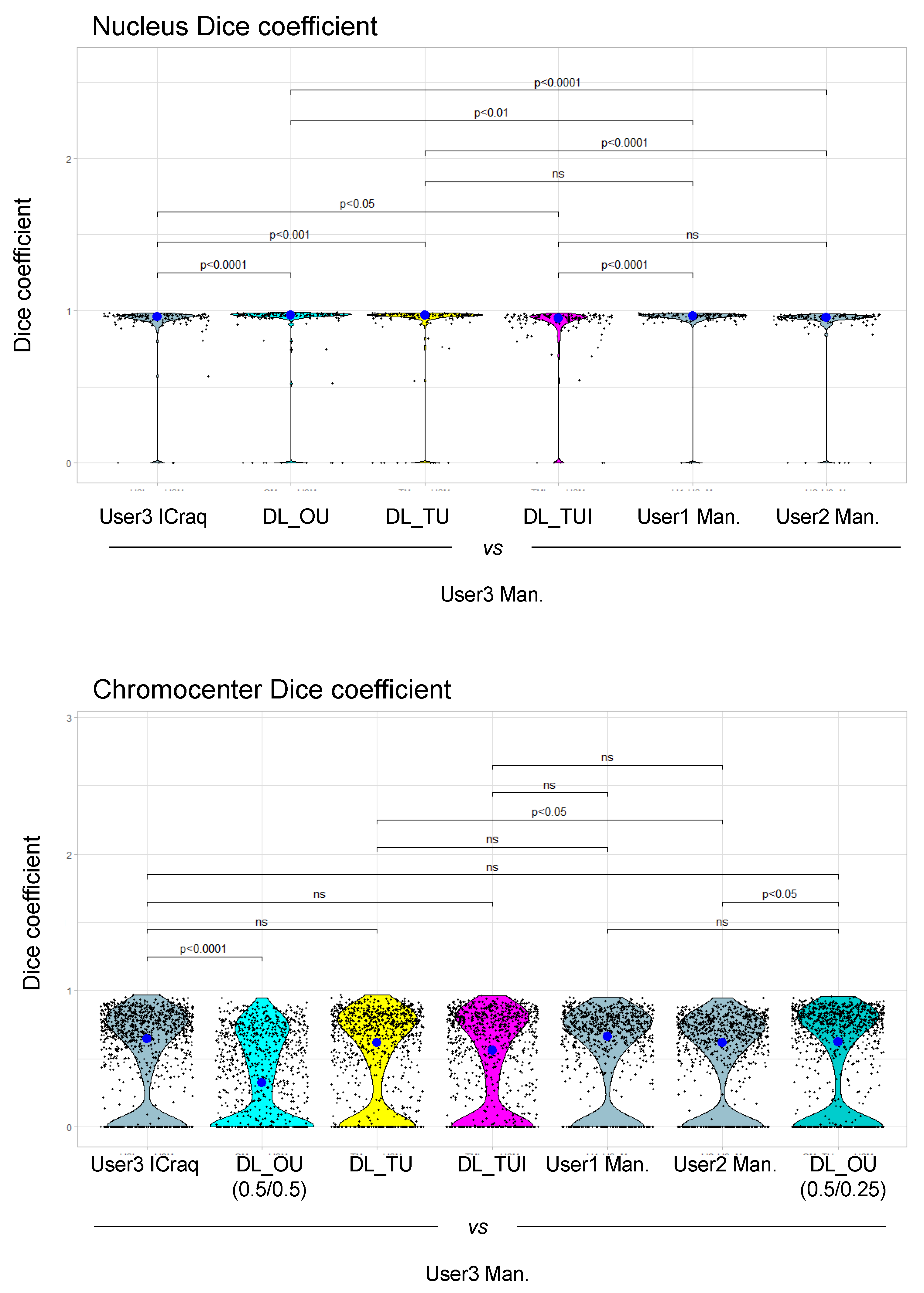
2.3. Nucl.Eye.D-Based Analysis of Nucleus and Chromocenters
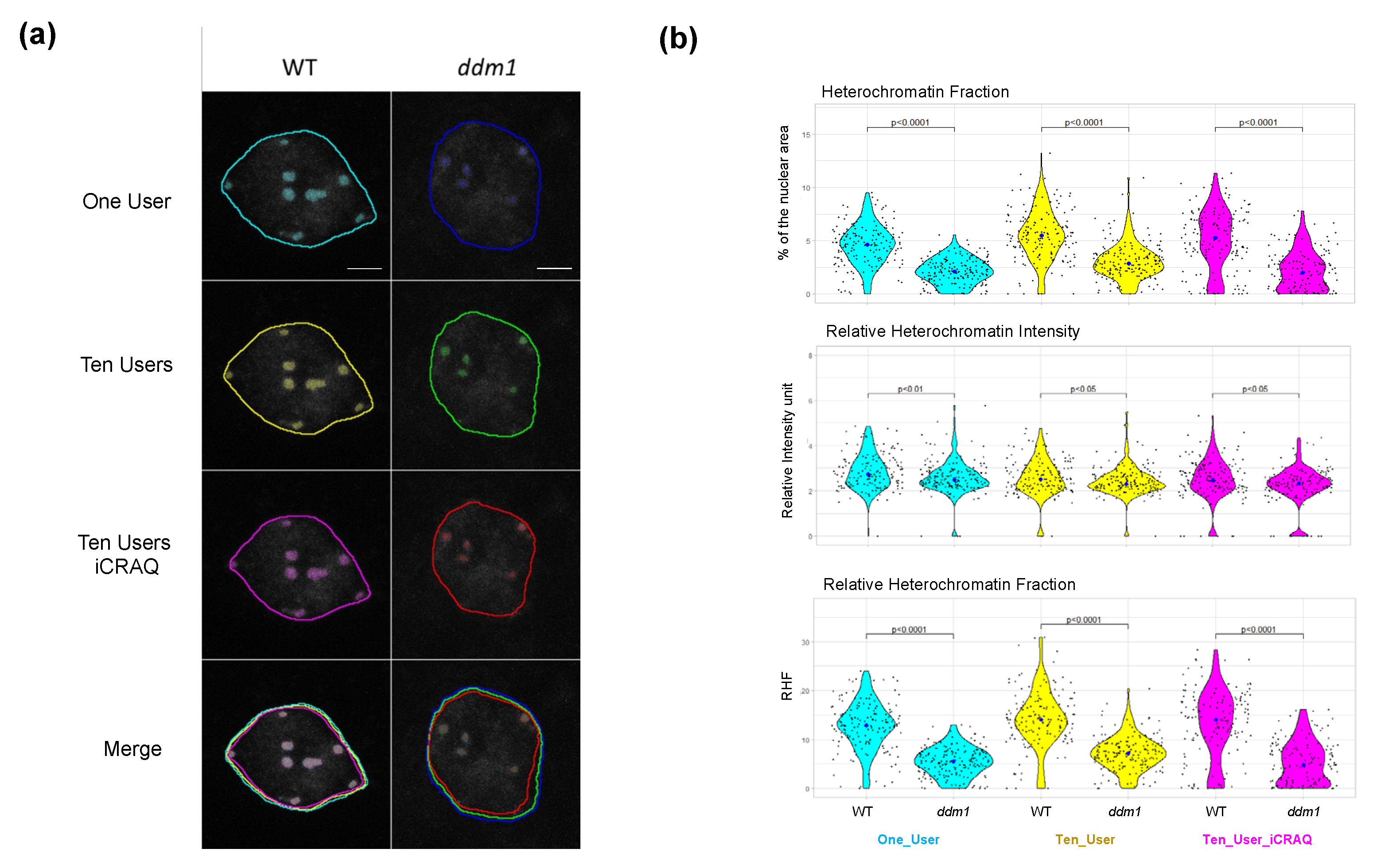
2.4. Nucl.Eye.D Analysis of the Ddm1 Dataset
3. Materials and Methods
3.1. Plant Material and Growth Conditions
3.2. Tissue Fixation and Nuclei Preparation for the Training Set
3.3. Tissue Fixation and Nuclei Preparation of Dark/Light Test Set
3.4. Mask Preparation
3.5. iCRAQ Analysis
3.6. Nucl.Eye.D
3.7. Morphometric Parameters Measurements
- -
- Relative CC area, also called relative CC area fraction (RAF): area of each CC/nucleus area
- -
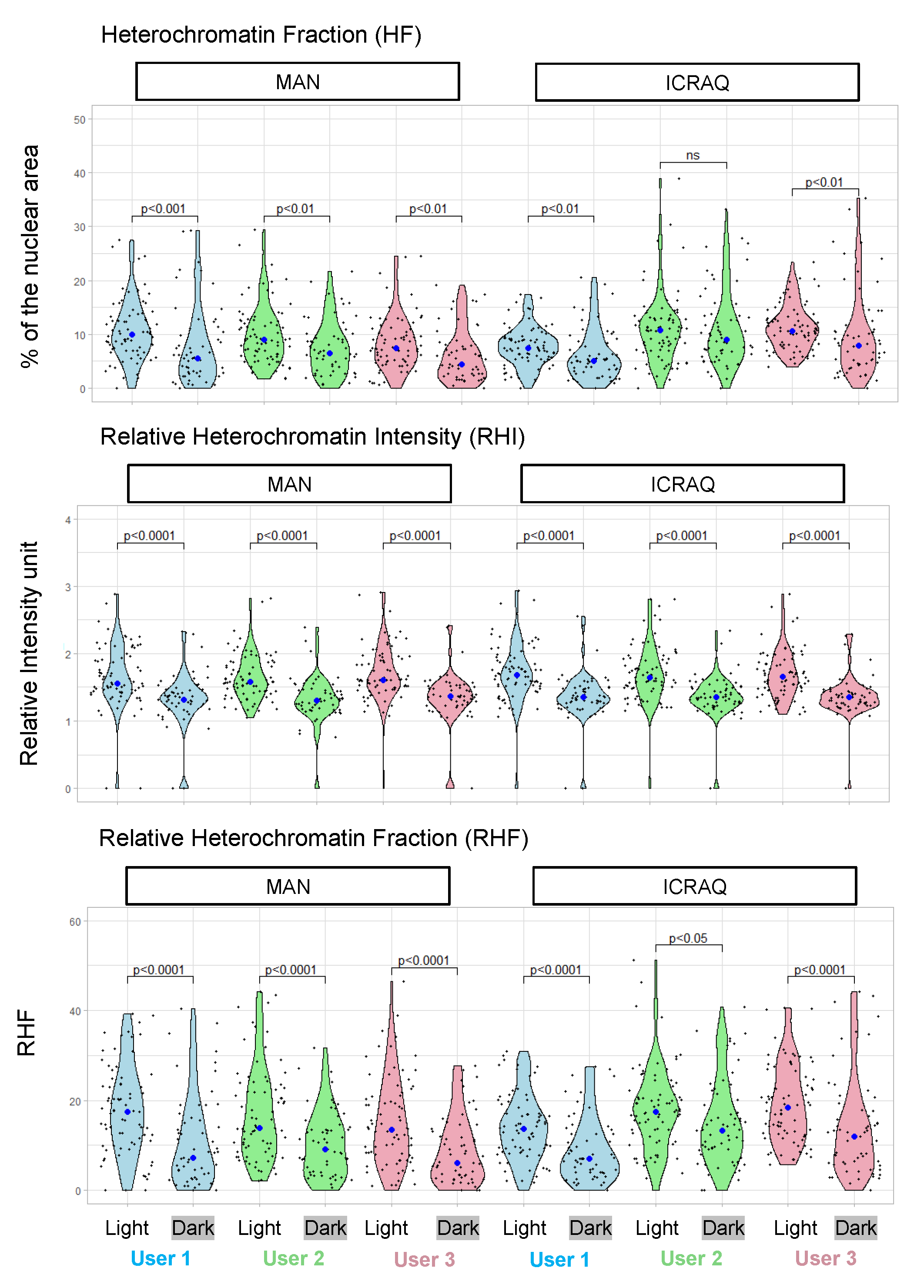
- Heterochromatin fraction (HF): sum of all chromocenters’ areas/nucleus area
- -
- Relative heterochromatin intensity (RHI): mean intensity of CC/mean intensity of nucleus
- -
- Relative heterochromatin fraction (RHF): HF × RHI
3.8. Data Display and Statistics
4. Conclusions
Supplementary Materials
Author Contributions
Funding
Institutional Review Board Statement
Informed Consent Statement
Acknowledgments
Conflicts of Interest
References
- Weigel, A.V.; Chang, C.-L.; Shtengel, G.; Xu, C.S.; Hoffman, D.P.; Freeman, M.; Iyer, N.; Aaron, J.; Khuon, S.; Bogovic, J.; et al. ER-to-Golgi Protein Delivery through an Interwoven, Tubular Network Extending from ER. Cell 2021, 184, 2412–2429.e16. [Google Scholar] [CrossRef] [PubMed]
- Keuenhof, K.S.; Larsson Berglund, L.; Malmgren Hill, S.; Schneider, K.L.; Widlund, P.O.; Nyström, T.; Höög, J.L. Large Organellar Changes Occur during Mild Heat Shock in Yeast. J. Cell Sci. 2022, 135, jcs258325. [Google Scholar] [CrossRef] [PubMed]
- Steblyanko, Y.; Rajendraprasad, G.; Osswald, M.; Eibes, S.; Jacome, A.; Geley, S.; Pereira, A.J.; Maiato, H.; Barisic, M. Microtubule Poleward Flux in Human Cells Is Driven by the Coordinated Action of Four Kinesins. EMBO J. 2020, 39, e105432. [Google Scholar] [CrossRef] [PubMed]
- Colombo, F.; Norton, E.G.; Cocucci, E. Microscopy Approaches to Study Extracellular Vesicles. Biochim. Biophys. Acta Gen. Subj. 2021, 1865, 129752. [Google Scholar] [CrossRef]
- Van Treeck, B.; Parker, R. Principles of Stress Granules Revealed by Imaging Approaches. Cold Spring Harb. Perspect Biol. 2019, 11, a033068. [Google Scholar] [CrossRef] [PubMed] [Green Version]
- Desset, S.; Poulet, A.; Tatout, C. Quantitative 3D Analysis of Nuclear Morphology and Heterochromatin Organization from Whole-Mount Plant Tissue Using NucleusJ. In Plant Chromatin Dynamics: Methods and Protocols; Bemer, M., Baroux, C., Eds.; Methods in Molecular Biology; Springer: New York, NY, USA, 2018; pp. 615–632. ISBN 978-1-4939-7318-7. [Google Scholar]
- Mikulski, P.; Schubert, D. Measurement of Arabidopsis Thaliana Nuclear Size and Shape. Methods Mol. Biol. 2020, 2093, 107–113. [Google Scholar] [CrossRef]
- Pavlova, P.; van Zanten, M.; Snoek, B.L.; de Jong, H.; Fransz, P. 2D Morphometric Analysis of Arabidopsis Thaliana Nuclei Reveals Characteristic Profiles of Different Cell Types and Accessions. Chromosome Res. 2021, 30, 5–224. [Google Scholar] [CrossRef] [PubMed]
- Arpòn, J.; Sakai, K.; Gaudin, V.; Andrey, P. Spatial Modeling of Biological Patterns Shows Multiscale Organization of Arabidopsis Thaliana Heterochromatin. Sci. Rep. 2021, 11, 323. [Google Scholar] [CrossRef] [PubMed]
- Simon, L.; Voisin, M.; Tatout, C.; Probst, A.V. Structure and Function of Centromeric and Pericentromeric Heterochromatin in Arabidopsis Thaliana. Front. Plant Sci. 2015, 6, 1049. [Google Scholar] [CrossRef] [Green Version]
- Fransz, P.; De Jong, J.H.; Lysak, M.; Castiglione, M.R.; Schubert, I. Interphase Chromosomes in Arabidopsis Are Organized as Well Defined Chromocenters from Which Euchromatin Loops Emanate. Proc. Natl. Acad Sci. USA 2002, 99, 14584–14589. [Google Scholar] [CrossRef]
- Almouzni, G.; Probst, A.V. Heterochromatin Maintenance and Establishment: Lessons from the Mouse Pericentromere. Nucleus 2011, 2, 332–338. [Google Scholar] [CrossRef] [PubMed] [Green Version]
- Schroeder, A.B.; Dobson, E.T.A.; Rueden, C.T.; Tomancak, P.; Jug, F.; Eliceiri, K.W. The ImageJ Ecosystem: Open-Source Software for Image Visualization, Processing, and Analysis. Protein Sci. 2021, 30, 234–249. [Google Scholar] [CrossRef]
- Landini, G.; Randell, D.A.; Fouad, S.; Galton, A. Automatic Thresholding from the Gradients of Region Boundaries. J. Microsc. 2017, 265, 185–195. [Google Scholar] [CrossRef] [PubMed] [Green Version]
- Zhang, J.; Li, C.; Rahaman, M.M.; Yao, Y.; Ma, P.; Zhang, J.; Zhao, X.; Jiang, T.; Grzegorzek, M. A Comprehensive Review of Image Analysis Methods for Microorganism Counting: From Classical Image Processing to Deep Learning Approaches. Artif. Intell. Rev. 2021, 55, 2875–2944. [Google Scholar] [CrossRef]
- Hunt, G.J.; Dane, M.A.; Korkola, J.E.; Heiser, L.M.; Gagnon-Bartsch, J.A. Automatic Transformation and Integration to Improve Visualization and Discovery of Latent Effects in Imaging Data. J. Comput. Graph. Stat. 2020, 29, 929–941. [Google Scholar] [CrossRef]
- Dubos, T.; Poulet, A.; Gonthier-Gueret, C.; Mougeot, G.; Vanrobays, E.; Li, Y.; Tutois, S.; Pery, E.; Chausse, F.; Probst, A.V.; et al. Automated 3D Bio-Imaging Analysis of Nuclear Organization by NucleusJ 2.0. Nucleus 2020, 11, 315–329. [Google Scholar] [CrossRef]
- Dubos, T.; Poulet, A.; Thomson, G.; Péry, E.; Chausse, F.; Tatout, C.; Desset, S.; van Wolfswinkel, J.C.; Jacob, Y. NODeJ: An ImageJ Plugin for 3D Segmentation of Nuclear Objects. BMC Bioinform. 2022, 23, 216. [Google Scholar] [CrossRef] [PubMed]
- Sensakovic, W.F.; Starkey, A.; Roberts, R.; Straus, C.; Caligiuri, P.; Kocherginsky, M.; Armato, S.G. The Influence of Initial Outlines on Manual Segmentation. Med. Phys. 2010, 37, 2153–2158. [Google Scholar] [CrossRef] [Green Version]
- Renard, F.; Guedria, S.; Palma, N.D.; Vuillerme, N. Variability and Reproducibility in Deep Learning for Medical Image Segmentation. Sci. Rep. 2020, 10, 13724. [Google Scholar] [CrossRef]
- Seeland, M.; Rzanny, M.; Boho, D.; Wäldchen, J.; Mäder, P. Image-Based Classification of Plant Genus and Family for Trained and Untrained Plant Species. BMC Bioinform. 2019, 20, 4. [Google Scholar] [CrossRef]
- Krull, A.; Buchholz, T.-O.; Jug, F. Noise2Void—Learning Denoising From Single Noisy Images. In Proceedings of the 2019 IEEE/CVF Conference on Computer Vision and Pattern Recognition (CVPR), Long Beach, CA, USA, 15–20 June 2019; pp. 2124–2132. [Google Scholar]
- Zhou, W.; Yang, Y.; Yu, C.; Liu, J.; Duan, X.; Weng, Z.; Chen, D.; Liang, Q.; Fang, Q.; Zhou, J.; et al. Ensembled Deep Learning Model Outperforms Human Experts in Diagnosing Biliary Atresia from Sonographic Gallbladder Images. Nat. Commun. 2021, 12, 1259. [Google Scholar] [CrossRef] [PubMed]
- Godec, P.; Pančur, M.; Ilenič, N.; Čopar, A.; Stražar, M.; Erjavec, A.; Pretnar, A.; Demšar, J.; Starič, A.; Toplak, M.; et al. Democratized Image Analytics by Visual Programming through Integration of Deep Models and Small-Scale Machine Learning. Nat. Commun. 2019, 10, 4551. [Google Scholar] [CrossRef] [Green Version]
- Gómez-de-Mariscal, E.; García-López-de-Haro, C.; Ouyang, W.; Donati, L.; Lundberg, E.; Unser, M.; Muñoz-Barrutia, A.; Sage, D. DeepImageJ: A User-Friendly Environment to Run Deep Learning Models in ImageJ. Nat. Methods 2021, 18, 1192–1195. [Google Scholar] [CrossRef] [PubMed]
- Shepley, A.; Falzon, G.; Lawson, C.; Meek, P.; Kwan, P. U-Infuse: Democratization of Customizable Deep Learning for Object Detection. Sensors 2021, 21, 2611. [Google Scholar] [CrossRef] [PubMed]
- Atanbori, J.; French, A.P.; Pridmore, T.P. Towards Infield, Live Plant Phenotyping Using a Reduced-Parameter CNN. Mach. Vis. Appl. 2020, 31, 2. [Google Scholar] [CrossRef] [PubMed] [Green Version]
- Yasrab, R.; Atkinson, J.A.; Wells, D.M.; French, A.P.; Pridmore, T.P.; Pound, M.P. RootNav 2.0: Deep Learning for Automatic Navigation of Complex Plant Root Architectures. Gigascience 2019, 8, giz123. [Google Scholar] [CrossRef] [PubMed] [Green Version]
- Li, S.; Li, L.; Fan, W.; Ma, S.; Zhang, C.; Kim, J.C.; Wang, K.; Russinova, E.; Zhu, Y.; Zhou, Y. LeafNet: A Tool for Segmenting and Quantifying Stomata and Pavement Cells. Plant Cell 2022, 34, koac021. [Google Scholar] [CrossRef] [PubMed]
- Li, J.; Peng, J.; Jiang, X.; Rea, A.C.; Peng, J.; Hu, J. DeepLearnMOR: A Deep-Learning Framework for Fluorescence Image-Based Classification of Organelle Morphology. Plant Physiol. 2021, 186, 1786–1799. [Google Scholar] [CrossRef] [PubMed]
- Tatout, C.; Mougeot, G.; Parry, G.; Baroux, C.; Pradillo, M.; Evans, D. The INDEPTH (Impact of Nuclear Domains On Gene Expression and Plant Traits) Academy—A Community Resource for Plant Science. J. Exp. Bot. 2022, 73, erac005. [Google Scholar] [CrossRef]
- Brändle, F.; Frühbauer, B.; Jagannathan, M. Principles and Functions of Pericentromeric Satellite DNA Clustering into Chromocenters. Semin. Cell Dev. Biol. 2022, 128, 26–39. [Google Scholar] [CrossRef] [PubMed]
- Goto, C.; Hara-Nishimura, I.; Tamura, K. Regulation and Physiological Significance of the Nuclear Shape in Plants. Front. Plant Sci. 2021, 12, 673905. [Google Scholar] [CrossRef]
- Pecinka, A.; Chevalier, C.; Colas, I.; Kalantidis, K.; Varotto, S.; Krugman, T.; Michailidis, C.; Vallés, M.-P.; Muñoz, A.; Pradillo, M. Chromatin Dynamics during Interphase and Cell Division: Similarities and Differences between Model and Crop Plants. J. Exp. Bot. 2020, 71, 5205–5222. [Google Scholar] [CrossRef]
- Bourbousse, C.; Mestiri, I.; Zabulon, G.; Bourge, M.; Formiggini, F.; Koini, M.A.; Brown, S.C.; Fransz, P.; Bowler, C.; Barneche, F. Light Signaling Controls Nuclear Architecture Reorganization during Seedling Establishment. Proc. Natl. Acad Sci. USA 2015, 112, E2836–E2844. [Google Scholar] [CrossRef] [Green Version]
- Benoit, M.; Layat, E.; Tourmente, S.; Probst, A.V. Heterochromatin Dynamics during Developmental Transitions in Arabidopsis—a Focus on Ribosomal DNA Loci. Gene 2013, 526, 39–45. [Google Scholar] [CrossRef]
- Pecinka, A.; Dinh, H.Q.; Baubec, T.; Rosa, M.; Lettner, N.; Scheid, O.M. Epigenetic Regulation of Repetitive Elements Is Attenuated by Prolonged Heat Stress in Arabidopsis. Plant Cell 2010, 22, 3118–3129. [Google Scholar] [CrossRef] [Green Version]
- Graindorge, S.; Cognat, V.; Johann to Berens, P.; Mutterer, J.; Molinier, J. Photodamage Repair Pathways Contribute to the Accurate Maintenance of the DNA Methylome Landscape upon UV Exposure. PLoS Genet. 2019, 15, e1008476. [Google Scholar] [CrossRef]
- Schindelin, J.; Arganda-Carreras, I.; Frise, E.; Kaynig, V.; Longair, M.; Pietzsch, T.; Preibisch, S.; Rueden, C.; Saalfeld, S.; Schmid, B.; et al. Fiji: An Open-Source Platform for Biological-Image Analysis. Nat. Methods 2012, 9, 676–682. [Google Scholar] [CrossRef] [Green Version]
- Schivre, G. ICRAQ. 2022. Available online: https://github.com/gschivre/iCRAQ (accessed on 30 September 2022).
- Johann to Berens, P.; Theune, M. Nucl.Eye.D—Zenodo. 2022. Available online: https://zenodo.org/record/7075507 (accessed on 30 September 2022). [CrossRef]
- Vongs, A.; Kakutani, T.; Martienssen, R.A.; Richards, E.J. Arabidopsis Thaliana DNA Methylation Mutants. Science 1993, 260, 1926–1928. [Google Scholar] [CrossRef]
- Soppe, W.J.J.; Jasencakova, Z.; Houben, A.; Kakutani, T.; Meister, A.; Huang, M.S.; Jacobsen, S.E.; Schubert, I.; Fransz, P.F. DNA Methylation Controls Histone H3 Lysine 9 Methylation and Heterochromatin Assembly in Arabidopsis. EMBO J. 2002, 21, 6549–6559. [Google Scholar] [CrossRef]
- Li, C.H.; Tam, P.K.S. An Iterative Algorithm for Minimum Cross Entropy Thresholding. Pattern Recognit. Lett. 1998, 19, 771–776. [Google Scholar] [CrossRef]
- Cazes, M.; Franiatte, N.; Delmas, A.; André, J.-M.; Rodier, M.; Kaadoud, I.C. Evaluation of the Sensitivity of Cognitive Biases in the Design of Artificial Intelligence. In Proceedings of the Rencontres des Jeunes Chercheurs en Intelligence Artificielle (RJCIA’21) Plate-Forme Intelligence Artificielle (PFIA’21), Bordeaux, France, 1–2 July 2021; pp. 30–37. [Google Scholar]
- Alzubaidi, L.; Zhang, J.; Humaidi, A.J.; Al-Dujaili, A.; Duan, Y.; Al-Shamma, O.; Santamaría, J.; Fadhel, M.A.; Al-Amidie, M.; Farhan, L. Review of Deep Learning: Concepts, CNN Architectures, Challenges, Applications, Future Directions. J. Big Data 2021, 8, 53. [Google Scholar] [CrossRef]
- Paullada, A.; Raji, I.D.; Bender, E.M.; Denton, E.; Hanna, A. Data and Its (Dis)Contents: A Survey of Dataset Development and Use in Machine Learning Research. Patterns 2021, 2, 100336. [Google Scholar] [CrossRef]
- Ronneberger, O.; Fischer, P.; Brox, T. U-Net: Convolutional Networks for Biomedical Image Segmentation. In MICCAI 2015. Lecture Notes in Computer Science; Springer: Cham, Switzerland, 2015; Volume 9351. [Google Scholar]
- Mathieu, O.; Jasencakova, Z.; Vaillant, I.; Gendrel, A.-V.; Colot, V.; Schubert, I.; Tourmente, S. Changes in 5S RDNA Chromatin Organization and Transcription during Heterochromatin Establishment in Arabidopsis. Plant Cell 2003, 15, 2929–2939. [Google Scholar] [CrossRef] [Green Version]
- Snoek, B.L.; Pavlova, P.; Tessadori, F.; Peeters, A.J.M.; Bourbousse, C.; Barneche, F.; de Jong, H.; Fransz, P.F.; van Zanten, M. Genetic Dissection of Morphometric Traits Reveals That Phytochrome B Affects Nucleus Size and Heterochromatin Organization in Arabidopsis Thaliana. G3 Bethesda 2017, 7, 2519–2531. [Google Scholar] [CrossRef] [Green Version]
- RStudio. Open Source & Professional Software for Data Science Teams—RStudio. Available online: https://www.rstudio.com/ (accessed on 9 June 2022).
- Van Voorst, H.; Konduri, P.R.; van Poppel, L.M.; van der Steen, W.; van der Sluijs, P.M.; Slot, E.M.H.; Emmer, B.J.; van Zwam, W.H.; Roos, Y.B.W.E.M.; Majoie, C.B.L.M.; et al. Unsupervised Deep Learning for Stroke Lesion Segmentation on Follow-up CT Based on Generative Adversarial Networks. Am. J. Neuroradiol. 2022, 43, 1107–1114. [Google Scholar] [CrossRef]
- Wang, K.; Zhan, B.; Zu, C.; Wu, X.; Zhou, J.; Zhou, L.; Wang, Y. Semi-Supervised Medical Image Segmentation via a Tripled-Uncertainty Guided Mean Teacher Model with Contrastive Learning. Med. Image Anal. 2022, 79, 102447. [Google Scholar] [CrossRef]
- Stringer, C.; Wang, T.; Michaelos, M.; Pachitariu, M. Cellpose: A Generalist Algorithm for Cellular Segmentation. Nat. Methods 2021, 18, 100–106. [Google Scholar] [CrossRef]
- von Chamier, L.; Laine, R.F.; Jukkala, J.; Spahn, C.; Krentzel, D.; Nehme, E.; Lerche, M.; Hernández-Pérez, S.; Mattila, P.K.; Karinou, E.; et al. Democratising Deep Learning for Microscopy with ZeroCostDL4Mic. Nat. Commun. 2021, 12, 2276. [Google Scholar] [CrossRef]
- Sun, W.; Nasraoui, O.; Shafto, P. Evolution and Impact of Bias in Human and Machine Learning Algorithm Interaction. PLoS ONE 2020, 15, e0235502. [Google Scholar] [CrossRef]
- Robinson, R.; Valindria, V.V.; Bai, W.; Oktay, O.; Kainz, B.; Suzuki, H.; Sanghvi, M.M.; Aung, N.; Paiva, J.M.; Zemrak, F.; et al. Automated Quality Control in Image Segmentation: Application to the UK Biobank Cardiovascular Magnetic Resonance Imaging Study. J. Cardiovasc. Magn. Reson. 2019, 21, 18. [Google Scholar] [CrossRef]


Publisher’s Note: MDPI stays neutral with regard to jurisdictional claims in published maps and institutional affiliations. |
© 2022 by the authors. Licensee MDPI, Basel, Switzerland. This article is an open access article distributed under the terms and conditions of the Creative Commons Attribution (CC BY) license (https://creativecommons.org/licenses/by/4.0/).
Share and Cite
Johann to Berens, P.; Schivre, G.; Theune, M.; Peter, J.; Sall, S.O.; Mutterer, J.; Barneche, F.; Bourbousse, C.; Molinier, J. Advanced Image Analysis Methods for Automated Segmentation of Subnuclear Chromatin Domains. Epigenomes 2022, 6, 34. https://doi.org/10.3390/epigenomes6040034
Johann to Berens P, Schivre G, Theune M, Peter J, Sall SO, Mutterer J, Barneche F, Bourbousse C, Molinier J. Advanced Image Analysis Methods for Automated Segmentation of Subnuclear Chromatin Domains. Epigenomes. 2022; 6(4):34. https://doi.org/10.3390/epigenomes6040034
Chicago/Turabian StyleJohann to Berens, Philippe, Geoffrey Schivre, Marius Theune, Jackson Peter, Salimata Ousmane Sall, Jérôme Mutterer, Fredy Barneche, Clara Bourbousse, and Jean Molinier. 2022. "Advanced Image Analysis Methods for Automated Segmentation of Subnuclear Chromatin Domains" Epigenomes 6, no. 4: 34. https://doi.org/10.3390/epigenomes6040034