1. Introduction
As the “workhorse” of the equipment manufacturing industry, machine tools are one of the most important tools in industrial production, with applications covering the mechanical industry, automotive industry, electric power equipment, railroad locomotives and aerospace. As the core component of machine tools, the operating condition of the spindle directly affects the machining accuracy and efficiency of machine tools, while the bearing, as the spindle support component of machine tools, directly affects the rotational accuracy of the spindle due to its assembly accuracy and the same of the enemy [
1,
2,
3]. Due to long-term service in variable loads, high temperatures, shock, and other harsh environments, and by manufacturing errors, assembly accuracy and human operation errors, and other factors, will lead to bearing deflection in the service process, which is very easy to cause bearing failure. Therefore, accurate and efficient real-time condition monitoring of bearings is important to ensure the healthy operation of machine tools and improve productivity [
4].
Traditional bearing condition monitoring methods are often studied with the help of time-domain features of the signal, and a few methods consider feature extraction in both frequency and time-frequency domains and use the extracted feature information for condition monitoring [
5]. Previous mechanical fault diagnosis models based on deep learning have poor generalization ability and complex networks, Deng Mingyang et al. [
6] combined frequency domain feature extraction self-encoder with variational self-encoder and proposed frequency domain feature variational self-encoder, which makes the extracted features more robust. Using the overall similarity of the same mode class vibration observation samples on the FFT amplitude spectrum feature waveform, Jiao Weidong et al. [
7] proposed a fault diagnosis method based on the pattern matching of the frequency domain feature waveform. Kullbak-Leibler (KL) distance mutual parameter method can solve the blind deconvolution order uncertainty problem, Liu Feng [
8] et al. proposed an improved time domain blind deconvolution order uncertainty method based on the combination of generalized morphological filtering and improved KL distance combination of improved time-domain blind deconvolution fault feature extraction algorithm, and the method can effectively extract rolling bearing fault features. Weimin Li [
9] et al. proposed a diagnosis method based on a frequency-domain sparse classification algorithm, which effectively overcomes noise interference and avoids the problem of fault feature frequency estimation. For the cliffness, margin, and spectral cliffness, which are usually very sensitive to the data singularity of the signal due to chance factors, are easy to cause misjudgment in the condition monitoring of bearings, Wang Xiaoling [
10] et al. proposed a frequency band entropy method based on time-frequency analysis and information entropy theory for rolling bearing fault monitoring. In order to make comprehensive use of the time-frequency domain information of vibration signal and the complexity characteristics of measuring time-frequency distribution, Jiaqi Li et al. [
11] introduced two-dimensional multiscale entropy into the fault diagnosis of rolling bearings and proposed a rolling bearing fault diagnosis method based on two-dimensional time-frequency multiscale entropy and firefly algorithm optimized support vector machine. The above method only considers the fault feature extraction in the time domain, frequency domain, or time-frequency domain separately, which has certain limitations in bearing fault diagnosis and is difficult to reflect its fault state accurately, and it is difficult to guarantee the mapping relationship between its feature value and service state as the amount of data increases.
With the development of computer hardware, machine learning has become a very effective tool for classification, for which the classification problem is the basis and many applications have evolved from it. Machine learning is able to learn the laws and patterns of data with the help of computers in a large amount of data, and in the process of learning, the potential and valuable information within the data is mined deeply [
12,
13,
14]. In order to improve the monitoring speed and monitoring accuracy, many scholars have introduced machine learning methods into the field of condition monitoring and achieved good results. Traditional shallow machine learning methods include support vector machines, decision trees, K-nearest neighbors, plain Bayes, artificial neural networks, etc., which, due to their need for large amounts of prior knowledge, lead to difficult feature extraction and selection [
15,
16].
In recent years, under the impact of the wave of artificial intelligence, people have started to introduce end-to-end deep learning methods into the fault diagnosis collar, and deep learning models have provided new ideas for fault diagnosis research by getting rid of the inevitable uncertainty of manual feature extraction methods [
17]. A convolutional neural network (CNN) is a class of feedforward neural network that contains convolutional computation and has a deep structure, and is one of the representative algorithms of deep learning [
18]. The algorithm has the capability of representational learning and is able to classify the input information in a translation-invariant manner according to its hierarchical structure. Janssens [
19] proposed a three-layer CNN model for bearing fault detection using vibration signals, where a discrete Fourier transform is applied to the data before the model is trained and fed into the network model. Gu [
20] proposed to feed the original vibration signals into 1-DCNN and Gu [
21] proposed an improved convolutional neural network model with global mean pooling instead of the final fully connected layer of CNN for the purpose of reducing the number of parameters, which effectively improved the computational speed of the model. To address the problem that traditional fault diagnosis methods require manual feature extraction and feature information is difficult to be fully mined, Chen Ke et al. [
22] proposed an end-to-end bearing fault diagnosis method based on CNN, LSTM, and attention mechanism. To address the problem that the traditional bearing fault diagnosis method does not sufficiently extract key features under strong noise and variable load, Yang Xianglan et al. [
23] proposed an ECA_ResNet-based bearing fault diagnosis method.
As the layers of a neural network become deeper, the path from the output to the input becomes longer, which leads to the disappearance of the change gradient in the process of backpropagation back to the input. To address this problem, densely connected neural network (DenseNet), as an improved algorithm of the CNN network, solves this problem by establishing dense connections between all the previous layers and the later layers to reuse the features, and some research have been conducted by related scholars. Huang et al. [
24] proposed a densely connected convolutional network (DenseNet), which improves the learning efficiency by feature reuse. enhance the learning efficiency, which is the most advanced convolutional neural network architecture. c Shi [
25] proposed a wear-induced internal leakage fault diagnosis method based on intrinsic modal functions (IMFs) and weighted densely connected convolutional networks (WDenseNets), using the weighted optimal IMF components as inputs to WDenseNet for fault identification and classification. Yufeng Wang [
26] proposed an improved one-dimensional DenseNet network structure capable of handling one-dimensional spectral sequences to achieve multi-scale for signal feature extraction. Rexiang Niu et al. [
27] proposed an improved fault diagnosis method for densely connected convolutional networks, which extracts features through multi-scale convolutional layers and achieves weighting of multi-scale feature channels using an attention mechanism to improve the generalization performance of the model. Qingrong Wang et al. [
28] proposed a dual-channel cross-dense connected fault diagnosis model incorporating parallel ECA modules, and designed a multi-convolutional residual module and a multi-scale dense connected network for fault feature extraction to achieve interaction and integration of fault information. To address the problem of insufficient ability of shallow features to characterize the fault information of vibration signals, K. Wang et al. [
29] proposed an intelligent fault diagnosis neural network model combining a style recalibration module and a densely connected convolutional neural network. Some of the above methods do not give full play to the powerful feature extraction capability of the DenseNet network, the model network structure is shallow, the network generalization capability is weak, or the frequency domain and time-frequency domain signal feature extraction is not considered.
In summary, this paper proposes a method to evaluate the bearing load inhomogeneous operating state based on a dual-channel fusion improved DenseNet network, firstly, data enhancement is performed on the original sample data by overlapping sampling method; secondly, frequency domain and time-frequency domain transformations are performed on the processed data to obtain the experimental data set of two channels; then the processed experimental data are input into the improved 1D-DenseNet and 2D-DenseNet models for feature extraction; finally, the frequency-domain and time-frequency-domain features are fused by concat splicing operation to achieve the classification and recognition of the load inhomogeneity of bearings. The method uses densely connected networks to build the base model, which greatly increases the depth of the network structure and enhances the generalization ability of the model. The effectiveness of the proposed method is verified through experiments, which provides a new idea for rolling bearing fault diagnosis.
2. Fundamentals
2.1. Convolutional Neural Network
2.1.1. Principle of Convolutional Neural Network (CNN)
CNN is a supervised learning neural network with a multilayer convolutional structure, introduced by Hubel and Wiesel with the concept of Receptive fields [
30]. First proposed by LeCun for image processing [
31], it differs from the traditional neural network structure in that it consists of two main parts: a convolutional layer and a pooling layer. The convolutional layer is connected to the previous layer by local connectivity and weight sharing, which greatly reduces the number of required parameters; the downsampling layer is a method for feature dimensionality reduction, i.e., reducing the complexity of the network by reducing the input feature parameters, which not only improves the robustness of the neural network but also prevents the occurrence of overfitting [
32,
33].
The convolutional layer is the core of CNN, which mainly implements the feature extraction of the dataset, which is one of the most important differences from traditional neural networks. The features of each layer in the convolutional layer are obtained by convolving the convolutional kernel with the input features of the previous layer, and the parameters can be adjusted through training to obtain the optimal features. In practice, smaller convolutional kernels are used to reduce the amount of operations. Each convolutional kernel can be used as a tool for feature extraction, and a new feature map is generated by means of convolutional operations. The convolution operation is the process of letting the convolution kernel slide along the coordinate position of the input image or input signal horizontally or vertically for a certain number of steps to compute the data corresponding to it, and the computational equation is as follows [
34]:
where
M represents the set of input feature maps, ∗ represents the convolution operation,
k represents the convolution kernel,
b represents the bias term,
represents the
jth feature map of the
layer, and
represents the nonlinear activation function used to enhance the representation of the data.
Pooling layer, also known as downsampling layer, can reduce the dimensionality of the input feature set, reduce the computational effort of the neural network, and increase the perceptual field of the posterior neurons to achieve the effect of effective control of overfitting. The pooling operation can be divided into maximum pooling and average pooling, among which maximum pooling is more widely used. Maximum pooling plans the input features into several regions and outputs the maximum value of each region separately.
2.1.2. ResNet Network
As the depth of the network keeps increasing, CNN models begin to suffer from a series of problems such as gradient disappearance and explosion, which in turn lead to a decrease in the accuracy of the model. Based on this, He et al. [
35] proposed ResNet by borrowing the idea of cross-layer linking of high-speed networks, the core of which is the residual block. Since this network structure utilizes the residual technique, it is also known as the residual network, and the specific structure is shown in
Figure 1:
The structural expression of the residual network is as follows:
where
denotes the output of the structure,
denotes the input, and
denotes the output obtained from the convolution layer. When the parameter of the convolution layer is 0, the formula is expressed as
. This is the core idea of the residual network, which achieves the transfer of feature information of each layer by constant connection, which ensures the depth of the network and improves the performance of the network model at the same time.
2.2. DenseNet Network
A dense convolutional neural network is an improved convolutional neural network algorithm based on the residual network (ResNet), which aims to alleviate the problem of gradient disappearance and model degradation by using fewer parameters. The core idea of a dense convolutional network as a neural network with dense connectivity is cross-layer connectivity, where each layer of input in the network model takes as input the feature information output from all previous layers, while the features of that layer are also directly passed to all subsequent layers as input to ensure maximum information transfer between layers, making the network perform similar deep supervision in an implicit way [
24].
The DenseNet network proposes a new structure by multiplexing the features, which not only slows down the gradient disappearance, but also has a smaller number of parameters, and it is connected in the form of cross-channel with the formula:
where: is the input to the
network;
is the output of layer l in the network;
is the input to layer
l − 1 of the network.
is the nonlinear transformation operation acting on layer
l.
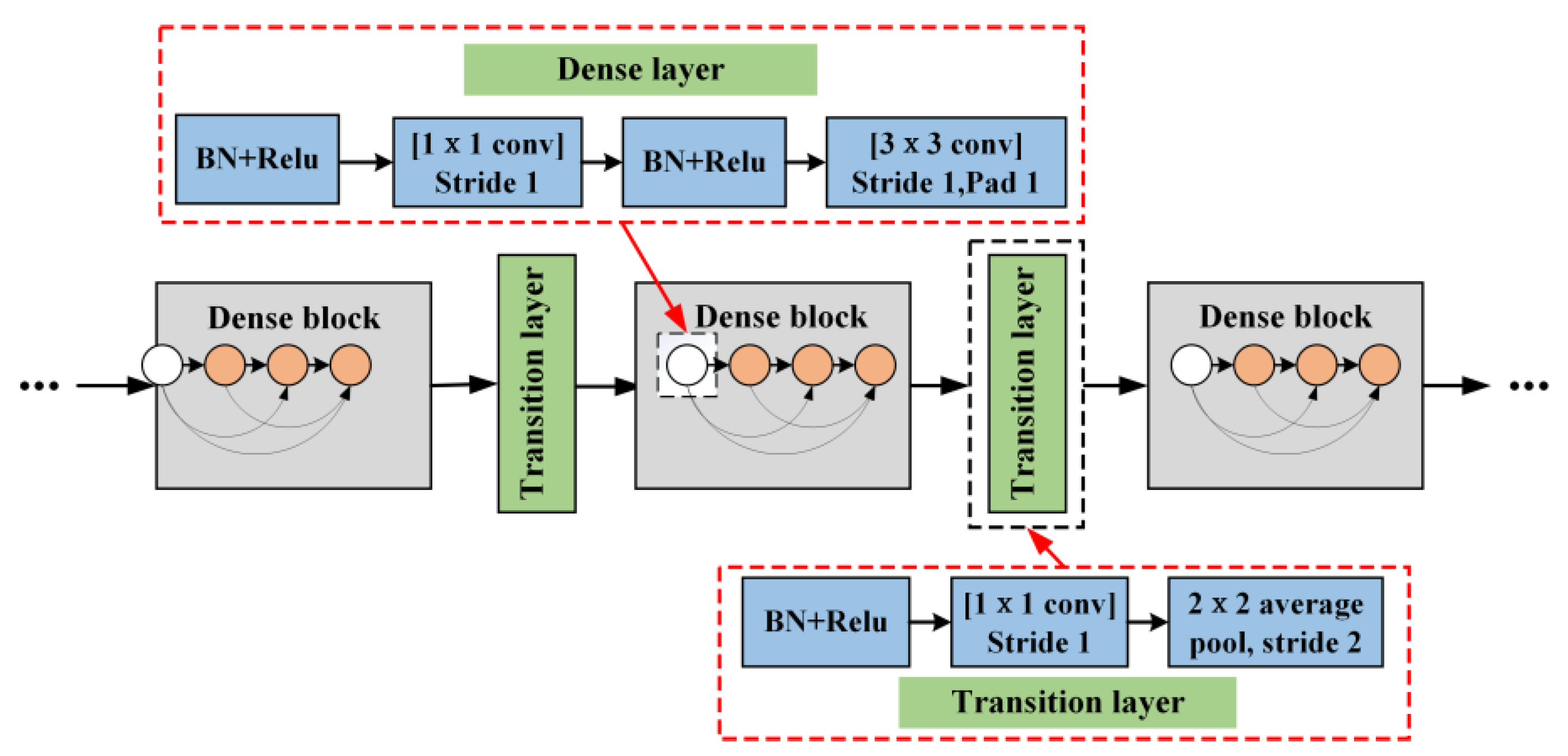
DenseNet mainly consists of convolutional layer, pooling layer, DenseBlock, TransitionLayer, and linear classification layer. As the network structure is based on dense connections between the layers, it is referred to as a densely connected network, as shown in
Figure 2.
GrowthRate: The hyperparameter k is the network growth rate, which refers to the number of feature maps produced by each layer. An important feature of DenseNet is that k is very small for each layer, because each layer can be connected to all feature maps in the dense blocks that exist in it. The growth rate controls how much global information is added at each layer, and this information can be called anywhere in the network, which is the biggest difference between DenseNet and traditional neural networks.
DenseBlock: The network perceives the feature information locally through the first convolutional layer initially. Next, the data enters the dense block. A bottleneck layer structure is BN-Relu-Conv(1 × 1)-BN-Relu-Conv(3 × 3), which becomes Densenet-B. Each bottleneck layer generally contains a 1 × 1 convolution and a 3 × 3 convolution. The former serves to effectively reduce the number of feature maps, reduce the computational effort and achieve feature fusion for each channel, while the latter serves to perform feature extraction. A dense block can be composed of multiple bottleneck layers.
TransitionLayer: The network structure between two dense blocks is called the transition layer, and its structure is BN-Relu-Conv-Dropout-Pooling, which generally consistsa of 1 × 1 convolution and 2 × 2 pooling layer, the main role is to reduce the number of feature maps. denotes the compression factor, generally . If the forward thickening block generates n layers of feature maps, in order to compress the data, after the transition block, the number of feature maps as the input of the next thickening block becomes .
2.3. ECA-Net Module
The input time-frequency maps are learned by 2D-DenseNet dense network to obtain a large number of features, and the ECA-Net attention mechanism module is introduced to improve the classification efficiency of the fusion model, enhance the overall channel features, and improve the model performance [
36].
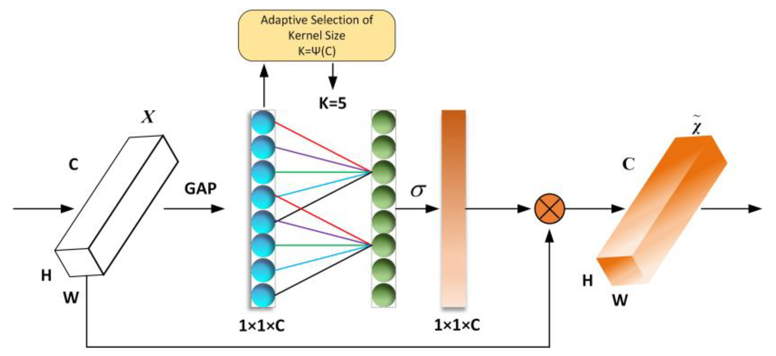
The ECA-Net attention mechanism uses the global average pooling layer directly after the convolutional layer, removing the fully connected layer. This module avoids dimensionality reduction and effectively captures cross-channel interactions. The module achieves good results with only a few parameters involved.
The ECA-Net module accomplishes cross-channel information interaction by one-dimensional convolution, and the size of the convolution kernel is adaptively varied by a function that allows more cross-channel interaction for layers with a larger number of channels, as shown in
Figure 3.
The adaptive function is as follows (where
):
The specific implementation process of the ECA-Net attention mechanism is as follows:
S1: Input feature maps with dimensions of .
S2: Perform spatial feature compression on the input feature map. Implementation: in the spatial dimension, using global average pooling GAP to obtain the feature map of .
S3: For the compressed feature map, channel feature learning is performed. Realization: through convolution, learning the importance between different channels, at this time the output dimension is still . The output dimension is still the same.
S4: Finally, the channel attention is combined with the feature map of channel attention , the original input feature map , perform channel-by-channel multiplication and finally outputs the feature map with channel attention.
According to the Efficient Channel Attention (ECA-Net) module shown in
Figure 3. Considering the aggregated features obtained through the global average library (GAP), ECA-Net generates channel weights by performing a fast one-dimensional convolution of size k, where k is determined adaptively by mapping the channel dimension C.
2.4. LSTM-Attention Module
The addition of the LSTM-Attention module to the 1D-DenseNet densely connected network can effectively suppress gradient disappearance or explosion with good generalization ability.
The LSTM network is improved from the standard RNN. The LSTM effectively alleviates the long-term dependence problem of the standard RNN through its internal complex gate operation and the introduction of cellular states [
37]. The unique feature of LSTM is that it introduces a memory cell and gate mechanism to solve the gradient disappearance and gradient explosion problems in the traditional RNN. LSTM is unique in that it introduces memory cell and gate mechanism to solve the gradient disappearance and gradient explosion problems in traditional RNNs, and enhances the ability to model long-term dependence.
The equations for the forgetting gate
, the input gate
, the output gate
, the cell state
and the output
are shown in the following equations:
where:
refers to the input at the current moment;
refers to the output at the previous moment;
refers to the weight matrix;
refers to the bias;
is the sigmoid activation function;
refers to the dot product operation.
Self-Attention is an improvement of the attention mechanism, which not only can quickly filter out the key information and reduce the attention to other irrelevant information, but also can reduce the dependence on external information and be better at capturing the internal relevance of the input data [
38]. By introducing the self-attention mechanism, the neural network solves the model information overload problem while also improving the accuracy and robustness of the network [
39].
The computation of Self-Attention is divided into two steps. Step 1: Calculate the attention weights between any vectors of the input sequence; Step 2: Calculate the weighted average of the input sequence based on the attention weights. The specific operation is shown in the following equation:
where:
Q,
K and
V are the query matrix, key matrix and value matrix, respectively, obtained by multiplying the input X with the corresponding weight matrices
,
,
, respectively; dim denotes the dimensionality of
Q,
K and
V.
In summary, vibration signal feature extraction by LSTM-Attention module can better capture the key features in the time series signal, and then improve the prediction accuracy of the model. This is very helpful for some application scenarios with high accuracy requirements, such as fault diagnosis and prediction.
3. Improved Evaluation Model of DenseNetnetwork Based Ontwo-Channel Fusion
3.1. Model Overview
In this paper, a dual-channel fusion DenseNet network model (Frequency and Time-Frequency domain fusion DenseNet, FTF-DFD) is constructed based on a densely connected neural network, and its structure is shown in
Figure 4: Since the original vibration data samples are insufficient and cannot be directly used in the standard network model to obtain better evaluation results, this paper performs data enhancement on the original data by overlapping sampling method.
The model shown in
Figure 4 is a two-channel DenseNet network structure consisting of the input layer, feature extraction module, and fault mode classification module. LSTM-Attention module for deep feature extraction; 1D-DenseNet model bottleneck layer structure is the same, both contain a combination of 1 × 1 and 1 × 3 size convolutional kernel, each dense block has a different number of bottleneck layers, this paper uses three groups of dense blocks, arranged according to the number of 3:2:1, adding a transition layer between every two dense blocks, which consists of a convolutional kernel size of 1 × 1 convolutional layer and a mean pooling layer of kernel size 1 × 2, which is used for downscaling and extracting global feature information, and finally, the output data of the network is linearized by squaring.
After the time domain signal is expanded by overlapping sampling, the wavelet time-frequency map is obtained by continuous wavelet transform, which is used as the input of the 2D-DenseNet model, and the ECA-Net attention mechanism is added after the last layer of dense blocks to effectively extract the model accuracy, strengthen the overall channel characteristics, and improve the model performance. The model structure of 2D-DenseNet is similar to that of 1D-DenseNet, which transforms the convolutional kernel from 1D to 2D, each bottleneck layer contains a combination of 1 × 1 and 3 × 3 size convolutional kernels, and the transition layer consists of a convolutional layer with 1 × 1 convolutional kernel size and an average pooling layer with 2 × 2 kernel size.
After the time-domain signal is overlapped sampled for data expansion, the wavelet time-frequency map is obtained by continuous wavelet transform, which is used as the input of the 2D-DenseNet model, and the ECA-Net attention mechanism is added after the last layer of dense blocks to effectively extract the model accuracy, strengthen the overall channel characteristics, and improve the model performance. 2D-DenseNet is similar to the model structure of 1D-DenseNet The model structure of 2D-DenseNet is similar to that of 1D-DenseNet, which transforms the convolutional kernel from 1D to 2D, each bottleneck layer contains a combination of 1 × 1 and 3 × 3 size convolutional kernels, and the transition layer consists of a convolutional layer with 1 × 1 convolutional kernel size and an average pooling layer with 2 × 2 kernel size.
The output feature data of the 1D-DenseNet model and 2D-DenseNet model are stretched into feature vectors, and the splicing operation is performed by concat, and the fused feature information is input into the fully connected network layer and SoftMax classifier, and the probability distribution belonging to each category is output to achieve the fault classification recognition of bearings. The frequency domain and time-frequency domain fusion method proposed in this paper has a good fusion effect and improves the classification accuracy of the model. The specific parameters of the model are shown in
Table 1.
3.2. Data Pre-Processing
3.2.1. Normalization Process
In order to data reduce the effect of distribution changes, improve the convergence speed of the model and diagnostic accuracy, the data are normalized and preprocessed, and the results are mapped to the [0–1] interval through a linear transformation, assuming that the sample data
, whose transformation equation is as follows.
where,
is the normalized result,
is the
i-th sample data,
is the maximum value of the sample data, and
is the minimum value of the sample data.
3.2.2. Data Enhancement
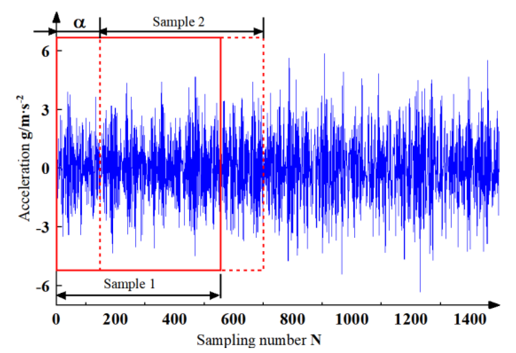
In the field of data-driven deep learning, having large enough training samples is the key to improve the accuracy of the model and effectively reduce the overfitting of the model. In this paper, we propose to increase the training samples by using overlapping sampling with moving sliding windows, as shown in
Figure 5, which can effectively increase the training samples while maintaining the periodicity and continuity of the one-dimensional time-series vibration signals and avoiding problems such as signal loss caused by isometric sampling and sampling.
From
Figure 5, if the total length of data in a certain state is
L = 245,759, the length of data for each sample is
= 1024. if no enhancement is applied, the number of samples
A that can be segmented by the current vibration signal is:
Using the moving sliding window overlap method with offset
= 100 for data sampling, the length of the overlapping part of the data is 924; the number of samples obtained from the current signal that can be split is (the maximum total number of samples that can be split per group of data is 2448)
Then the multiplier of sample expansion after using data enhancement
is
The expansion of the original data samples is achieved by overlapping sampling to avoid the loss of detailed features. Different offsets α, data lengths l, expansion multipliers γ and sample numbers B are set to achieve the performance detection of the model under different sample numbers and prove the practicality of the model.
3.2.3. Data Conversion
FFT is an efficient algorithm of Discrete Fourier Transform (DFT), called Fast Fourier Transform (FFT), which improves the DFT algorithm according to the odd, even, imaginary and real characteristics of DFT, and its basic principle is still Fourier Transform, which will not be discussed here. By calling the fft function in python, the frequency domain characteristics of the signal can be obtained, and then the frequency distribution of different signals can be analyzed.
The signal after data enhancement is analyzed in the time-frequency domain, where the time-frequency map of the original signal is obtained by continuous wavelet variation (CWT), which can clearly and accurately represent the time-frequency distribution of the vibration.
The continuous wavelet transform provides the best resolution results for non-periodic signals without leakage effects. Continuous wavelet transform
can be calculated by the following equation:
where,
is the scale,
s(
u) is the original signal,
is the translation, and
is the mother wavelet.
The continuous wavelet variation (Continuous Wavelet Transform, CWT) chooses Complex Morlet Wavelet (Cmor) as the wavelet basis, and the Cmor wavelet basis function is obtained by improving the Morlet wavelet basis function. It is a complex wavelet basis function with dual resolution properties in both frequency and time domains, which is widely used in the field of signal processing and wavelet analysis. The Cmor wavelet basis function has a similar shape to the Gaussian function but has better frequency localization properties in the frequency domain. It has better time-frequency localization properties in both time and frequency domains, and is suitable for processing non-stationary signals and analyzing transient phenomena in signals.
3.3. Model Training
The optimization algorithm used for the TADAT-based rolling bearing fault diagnosis model is chosen as Adam. The Adam algorithm adaptively adjusts the learning rate of each parameter, and different learning rates can be used for different parameters, thus making the training more efficient and stable.
The Adam algorithm dynamically corrects the training steps of each parameter using first-order moment estimation and second-order moment estimation of the gradient with the following update rules:
where,
denotes the model parameters at step
and step
, respectively;
is the learning rate;
denotes the value of the unbiased second-order moment estimate;
denotes the value of the unbiased first-order moment estimate; and
is a very small positive number, generally taken as
, preventing the denominator from being 0.
The TADAT-based rolling bearing fault diagnosis model diagnoses work conditions based on features, which belongs to the classification problem in supervised learning, so cross entropy is chosen as the loss function and optimized.
Cross entropy is mainly used to calculate the distance between the correct probability of labeling and the probability of prediction, and the smaller the value of cross entropy, the closer the prediction result is to the actual result, and the formula is as follows:
where,
denotes the individual learning parameters;
denotes the probability of correct labeling; and
is the prediction probability.
For two probability distributions
and
, define the K-L scatter of
and
as follows:
When calculating the cross-entropy loss using KL scatter, the true labels need to be transformed into probability distributions, usually using methods such as one-hot encoding or smoothed labels. In this paper, a smoothed target label is used instead of the traditional one-hot encoded label, thus reducing the impact of the noise and uncertainty of the label on the model and obtaining a loss function .
In
its L2 regularization penalty term is introduced to penalize the size of the model parameters to prevent overfitting. The strength of the regularization penalty can be controlled by adjusting the value of alpha to establish the regularized loss function as follows:
where,
denotes each learning parameter; alpha is the regularization parameter.
After pre-processing, the data set is divided into training set, validation set and test set in the ratio of 7:2:1, the model uses the parameters with the highest training and validation accuracy as the final parameters, the optimizer uses the Adam optimizer with fast and stable convergence, the loss function is the regularized loss function, the initial learning rate is 0.01, and the learning rate decays by half for every 10 iterations. Normalization batch normalization is used to accelerate the convergence speed of the neural network, Dropout operation is added to prevent overfitting, and the number of training iterations of the model is set to 100; finally, the Softmax function is used to classify the target and output the probability distribution of each category; as shown in
Table 2:
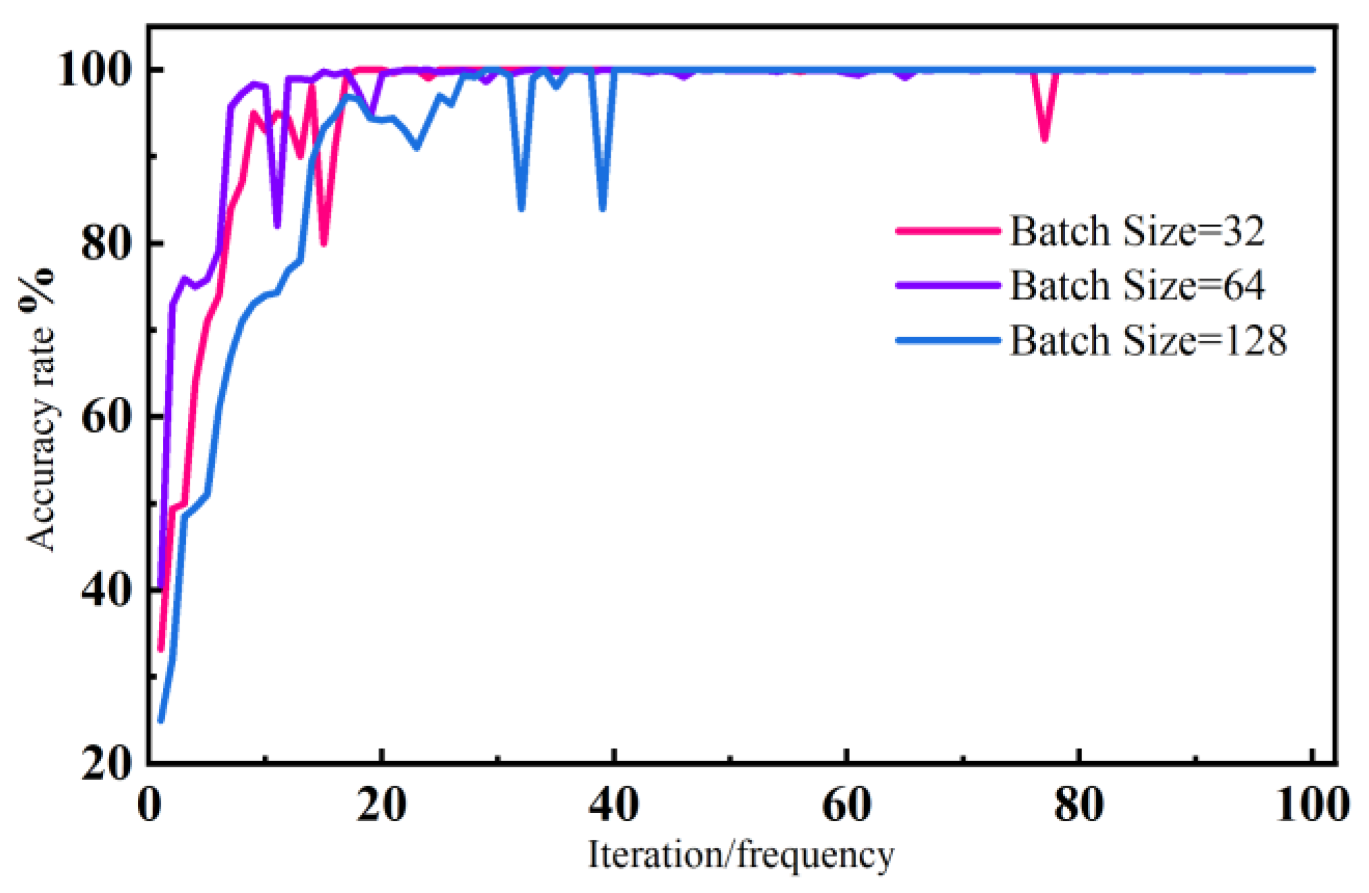
In order to obtain the appropriate Batch Size parameter for the model, the mid-load experiment was used as the basis for comparison by setting different Batch Size parameter values, mainly setting three different sets of values of 32, 64, and 128, as shown in
Figure 6, and it was found that the accuracy of the model improved the fastest when the Batch Size was set to 64, reaching 94% accuracy after 20 iterations, and After 60 iterations, the accuracy rate is stabilized at 100%, while the accuracy rate of the model test fluctuates more when the Batch Size is set to 32 and 128. It was concluded that the best iteration of model accuracy was achieved when the Batch Size was set to 64.
4. Experimental Verification
4.1. Environment Description
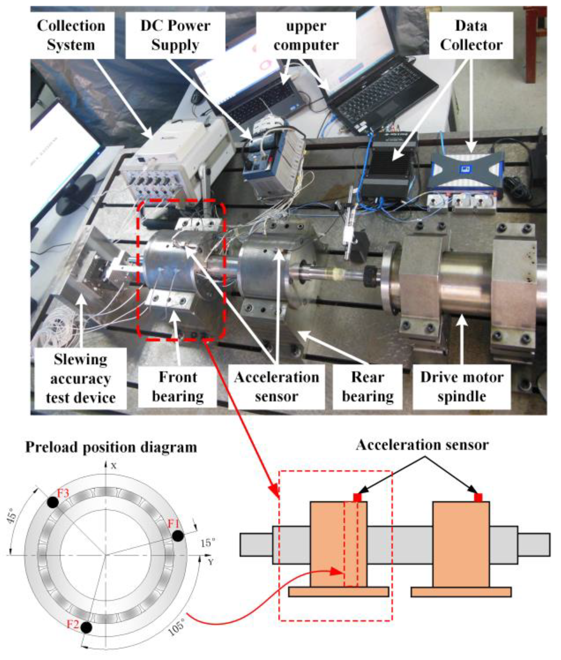
A non-equilibrium bearing load test stand was developed and built to further study the monitoring function of this technology in the process of double bearing operation, as shown in
Figure 7. The test stand mainly consists of a motor, a precision spindle, a rolling bearing and an acceleration sensor, and the maximum speed read by the electric spindle is 10,000 r/min. The mechanical spindle is connected to the electric spindle through a flexible coupling, and the motor operation is controlled by a servo control system.
The test rig used four NSK7014C angular contact ball bearings, where F1, F2 and F3 were loaded 120° on the bearings, respectively, and the bearing bias operating condition was determined by setting different sizes of preload; the bearings were mounted back-to-back with a fixed speed of 4000 r/min, a sampling frequency of 8192 Hz and a sampling length of 512.
Table 3 shows the bearing parameters.
Software environment: The training and testing environment of this paper is 14 cores, 16 G memory, processor: 12th Gen Intel Core i7-12700H processor; programming environment Pytorch1.7.1.
The bearing non-uniform load test bench is designed to distinguish the operating condition of the bearing under unbalanced operation, so that the bearing failure caused by factors such as assembly or machining can be detected in time. Due to the limited conditions in the laboratory, the currently built test bench can only be used to verify the effectiveness and accuracy of the condition monitoring method, and cannot simulate the corresponding bearing failure state for verification experiments.
4.2. Example Analysis
4.2.1. Data Conversion
A total of twelve sets of data are collected through the bearing load non-uniform operation fault simulation test bench, including F1, F2, F3 loading and data under even load conditions, which are mainly divided into four conditions of light load, medium load, heavy load and even load, and there are 12 types of bearing vibration data. There are four sets of experiments in total, the first three sets of experiments with 1400 samples in the training set, 400 samples in the test set and 200 samples in the validation set; the last set of experiments with all types of data input; the specific experimental data are shown in
Table 4.
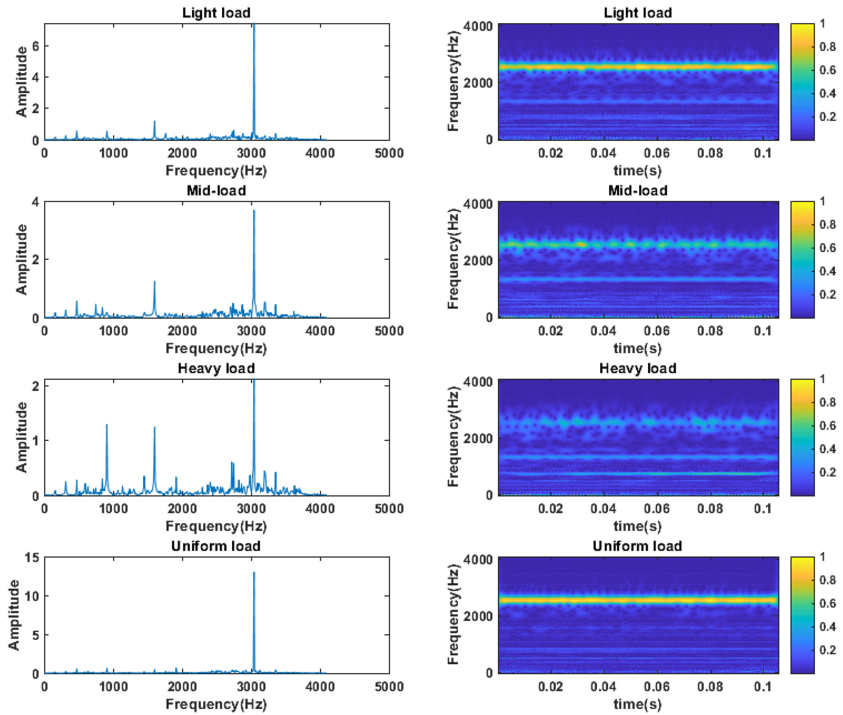
The vibration signals at F1 positions C2, C4, C6 and
(C1) working conditions were subjected to signal analysis, and 1024 data points were taken as one sample and subjected to FFT transform with wavelet transform. The analysis in
Figure 8 shows that the spectrograms of the four working conditions data at 3044 Hz have the maximum amplitude variation, which reflects the main frequency components of the signal in the frequency domain. As the load at the F1 position of the bearing gradually increases, the vibration characteristics of the bearing will be more intense, and more frequency components and amplitudes will be generated, and more noise and spurious frequencies may appear in the FFT analysis. Since the frequency and amplitude of the bearing vibration will change with the load, the amplitude of the main frequency components in the FFT spectrum is relatively small when the load is higher. Under the average load, the frequency and amplitude of bearing vibration are relatively stable, so the amplitude of the main frequency components in the FFT spectrum is relatively large. The spectrum analysis shows that the spectrum gradually increases with C6, C4, C2, and
(C1). The signal analysis of the time-frequency diagram also proves this point. In the energy distribution in the frequency range of 2 to 3 kHz, the
(C1) condition has the largest energy, while the C6 condition has the least energy.
4.2.2. Model Testing
The experiments were conducted with the input sample length of 1024, Batch Size of 64, training iterations of 100, learning rate of 0.002, and optimizer choice of Adam. The method was initially tested on the Case Western Reserve University bearing dataset.
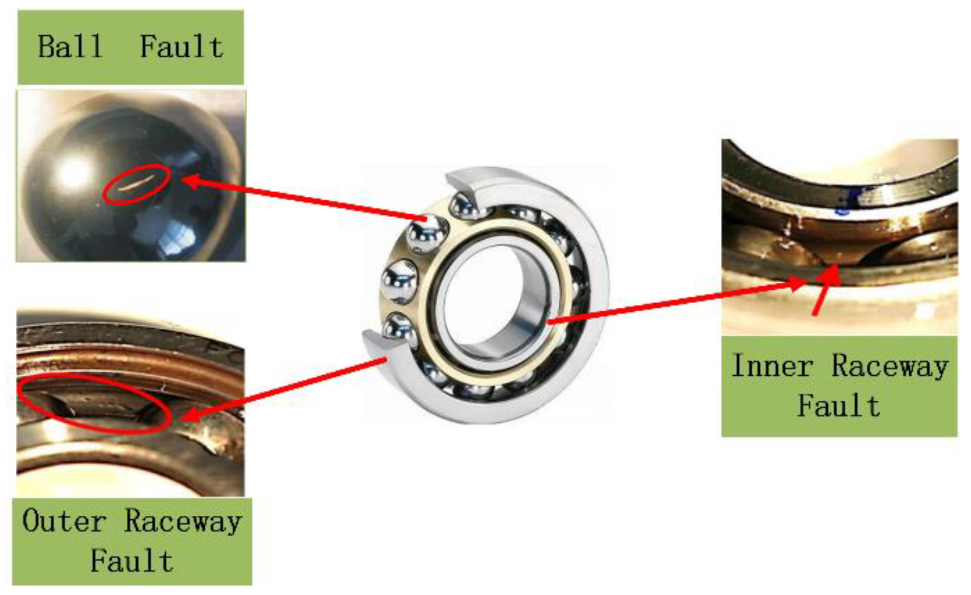
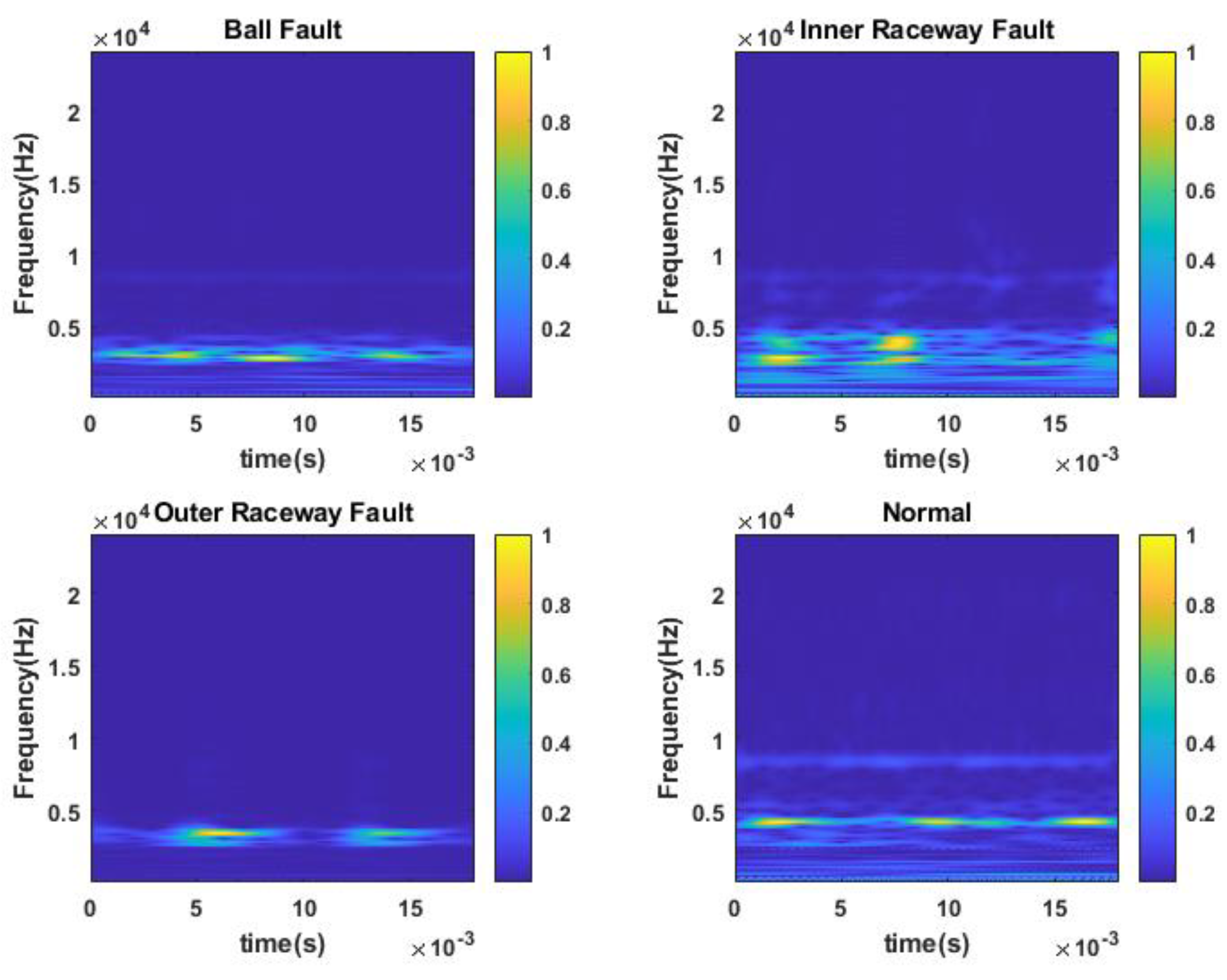
The test selected the bearing data at the drive end, sampling frequency of 48 kHz, and load of 0 hp, the fault form contains outer ring fault, inner ring fault and rolling body fault three kinds of fault parts as shown in
Figure 9, the fault type is specifically divided into 7 mils, 14 mils and 21 mils three kinds of fault diameter, plus the normal state, a total of ten kinds of bearing state data. The specific sample composition information is shown in
Table 5. A total of 70% of the samples are selected as the training set, 20% as the validation set, and 10% as the test set.
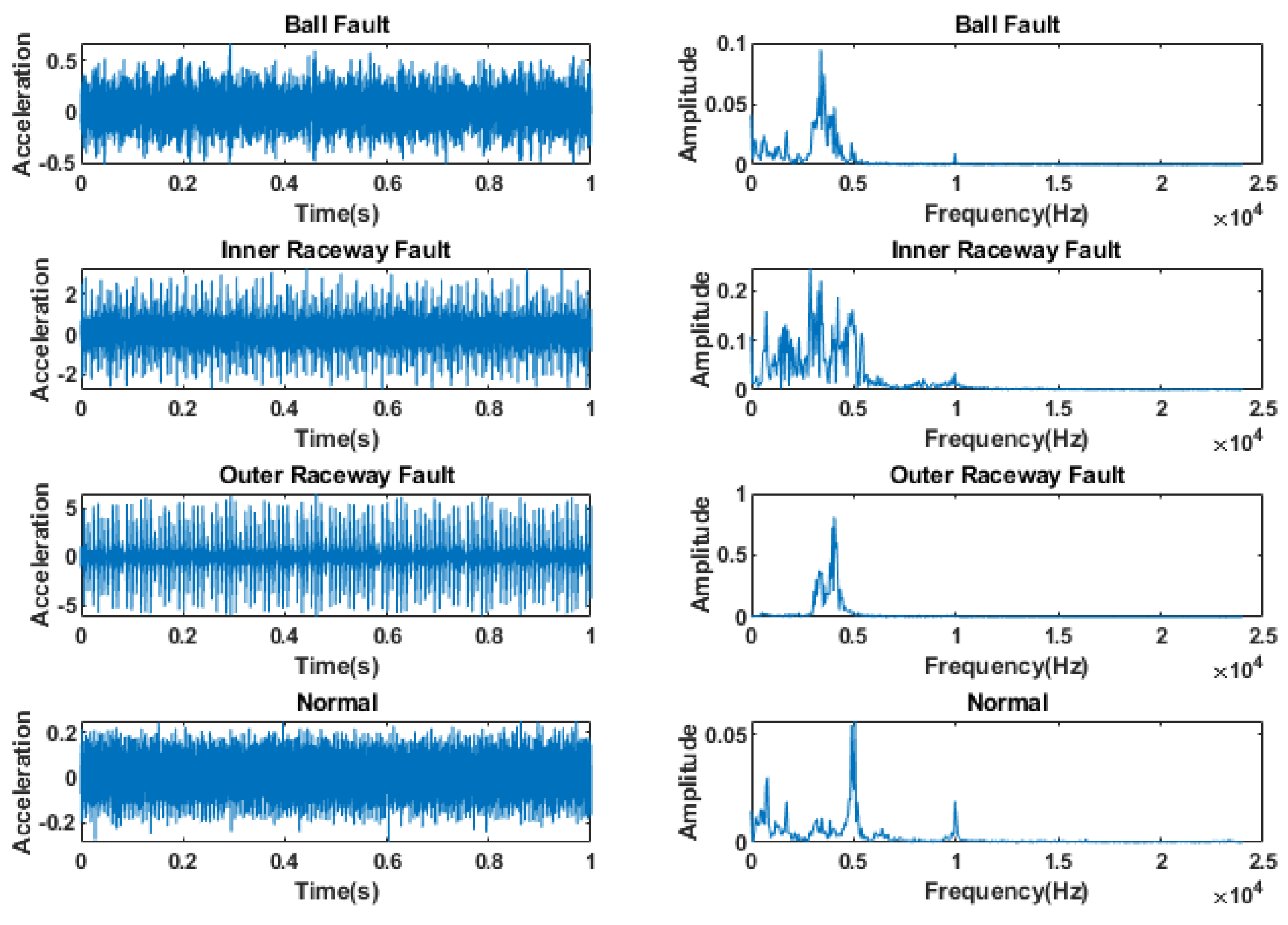
The time domain of the bearing vibration signal contains a large number of high and low-frequency components, which have different sensitivities for the diagnosis of bearing faults. Therefore, converting the time domain signal to the frequency domain signal for analysis can better capture the characteristics of bearing faults as shown in
Figure 10. The fault signal with fault type 7 mils at 0 hp is taken for spectral analysis with the normal signal, and 1024 data points are taken as a sample for FFT transformation, and four states of the bearing, such as normal state, rolling element fault, inner ring fault, and outer ring fault, can be found. The difference of amplitude in the high-frequency band is large.
Figure 11 shows that this mechanical vibration signal mainly contains energy in the frequency range of 0~5 kHz, in which the inner ring fault has obvious energy intensity transformation in both low and high-frequency bands, and its distribution is very dense because it is a different type of fault, which can effectively identify the frequency components and time domain features of the signal and provide useful information for applications such as signal feature extraction, classification, and diagnosis.
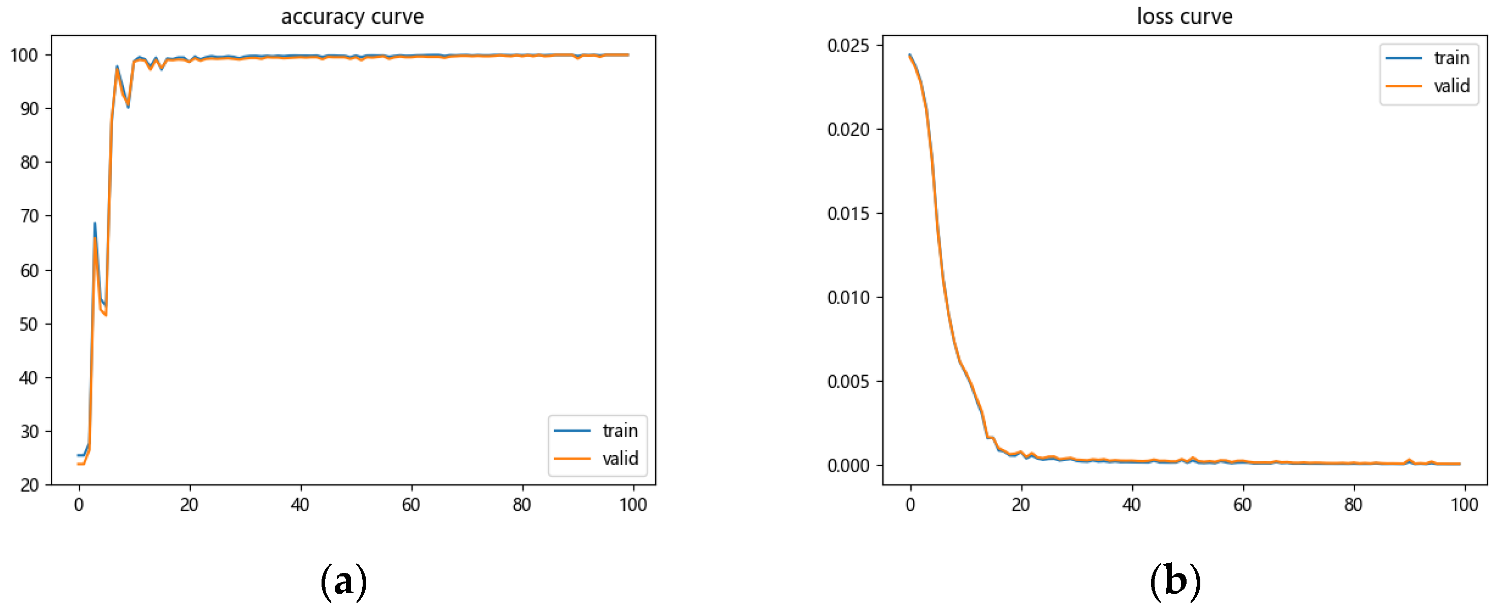
The ten bearing condition data in
Table 5 were input into the model for condition diagnosis of the bearings. From the model output accuracy versus loss function curve in
Figure 12, it can be seen that the model can reach 98% accuracy after 20 iterations, and after 50 iterations, the model can finally reach 100% accuracy.
In order to clearly represent the extraction ability of features in the model, we use the t-SNE technique to downscale and visualize the features in the input and output layers to indirectly represent the extraction ability of features in the model, where different colors and numbers indicate different fault categories and horizontal and vertical coordinates indicate different dimensions.
As shown in
Figure 13, the input layer is disorganized and various features are mixed together. After the three-stage densely connected network and the two-domain feature fusion, the extraction of features by the model is basically completed, and the separation and convergence of all kinds of features are basically completed, and the visual classification results of the output layer show that the model has a good classification effect.
4.3. Comparison Experiments
At the position of bearing F1, three working conditions of light load (OC_1), medium load (OC_2) and heavy load (OC_3) were measured, and three data sets M1, M2, and M3 were established to contain the information of the above three working conditions, and 300 samples were taken for each working condition. In the network model, the Batch Size is set to 64, the number of training iterations is set to 100, the optimizer is Adam, the initial learning rate is 0.01, and the learning rate decays by half every 10 iterations, and the loss function is selected as .
The diagnostic res CNN: The model structure is the input layer, Conv layer, MaxPool layer, ReLu activation function, BN layer, flat layer, Dropout layer, fully connected layer, and SoftMax output layer. The input data is a two-dimensional time-frequency map, and the middle layer is a two-layer convolutional pooling network, which is stretched by the flat layer and then passed through the fully-connected layer and the SoftMax output layer to achieve the classification of work conditions.
Improved-FTF-CNN: The model adopts the fusion of frequency domain and time-frequency domain, in which the 1D and 2D models, the three-level dense connection network is used, and the ratio of dense blocks are 3:2:1, relying on the feature fusion through concat, and finally the classification of working conditions through the SoftMax output layer.
DenseNet: The input layer of the model is fed with a two-dimensional time-frequency map, and the intermediate structure uses three groups of dense blocks, according to the number 3, 2, and 1. The output layer uses the SoftMax output layer for the classification of working conditions.
Improved-FTF-DenseNet: the base structure of the model is the same as the improved-FTF-CNN network structure, and the intermediate feature extraction structure replaces the CNN module in it with the DenseNet network structure, and the rest of the network results remain unchanged.
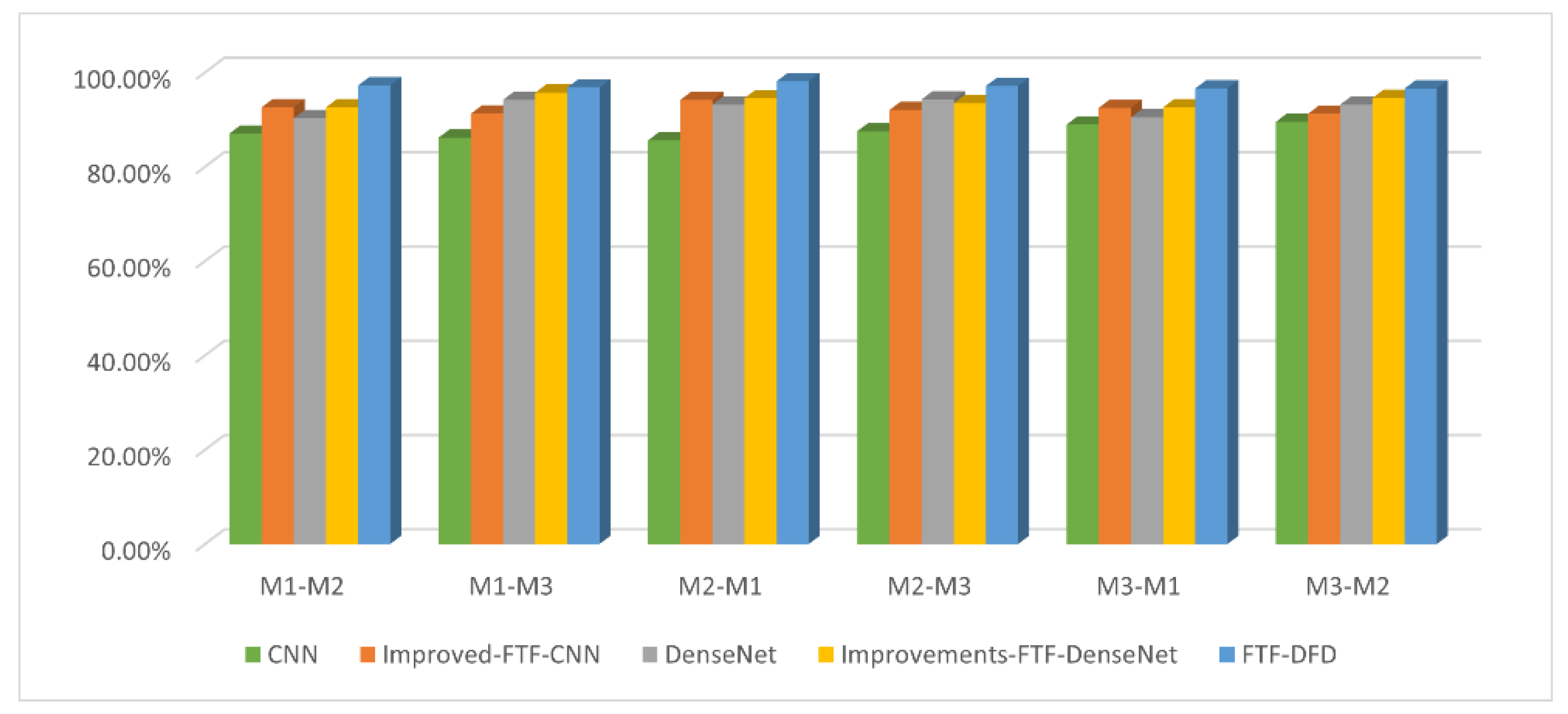
The diagnostic results of the above methods are shown in
Figure 14, and the average value of five experiments is taken as the model evaluation result, and the average value of six groups of experiments is taken for model performance evaluation, which is shown in
Table 6. the network structure of the CNN model is relatively simple and cannot extract accurate features, and the training time is the shortest, with an average accuracy rate of 87.43%; the improved-FTF-CNN model, compared with the simple CNN network, has an accuracy rate has significantly improved, and is 4.83% higher than the CNN model; the DenseNet model can improve the complexity of the model due to the dense connection structure, and after adjusting its parameters, the final accuracy can reach 92.57%; the improved-FTF-DenseNet can reach a final average accuracy of 93.88% through the model of dual-channel fusion, which is lower than the method of this paper by 3.18%.
4.4. Uneven Bearing Load Experiment
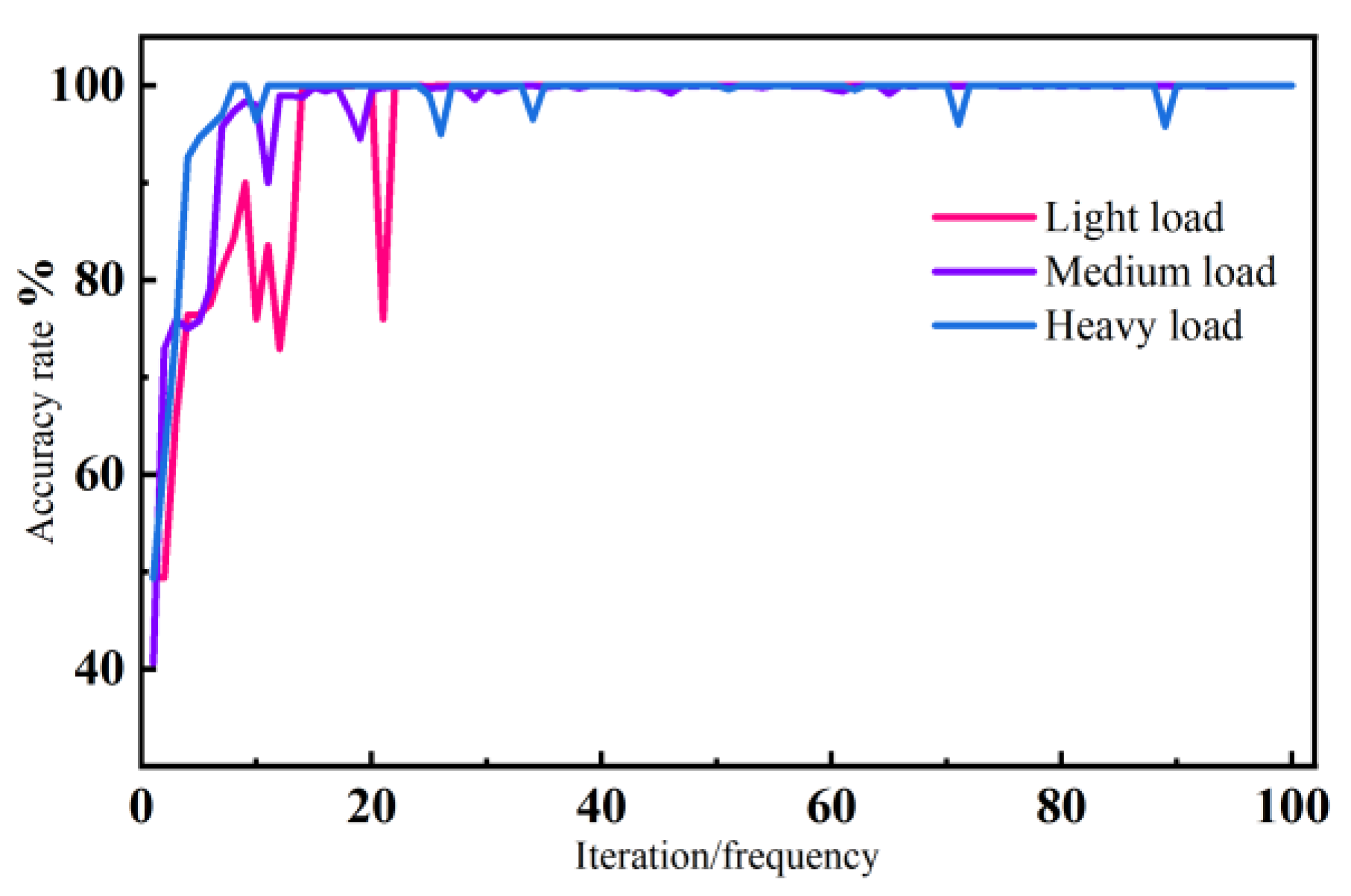
The results of three sets of experiments of the FTF-DFD fault diagnosis model proposed in this paper are shown in
Figure 15, which are the accuracy curves of the unbalanced experiments. The accuracy rates of the three different experimental conditions on the test set after 18 iterations of training all reach more than 98%, among which the accuracy curves of the light load experiments have a large abrupt change in the rising stage and the accuracy rate is not as fast as The accuracy curves of the medium-load and heavy-load experiments are not as fast as those of the medium-load and heavy-load experiments. The accuracy transformation curve is flatter under the medium-load experimental condition, and the accuracy can reach 100% on the test set after 50 iterations of training. The accuracy of all three unbalanced experiments reached 100% after 70 iterations of training, and it can be seen through the three sets of experiments that the model is more adaptable under medium-load and heavy-load working conditions.
The deeper the layers of the neural network model, the better the extraction effect for signal features. In this paper, the complexity of the model is increased by the densely connected network, and the learning ability of the model is enhanced to extract the one- and two-dimensional features of the original signal, and the model is made to obtain more feature information through the mode of two-channel fusion, so as to improve the accuracy of the model for monitoring the load inhomogeneous state.
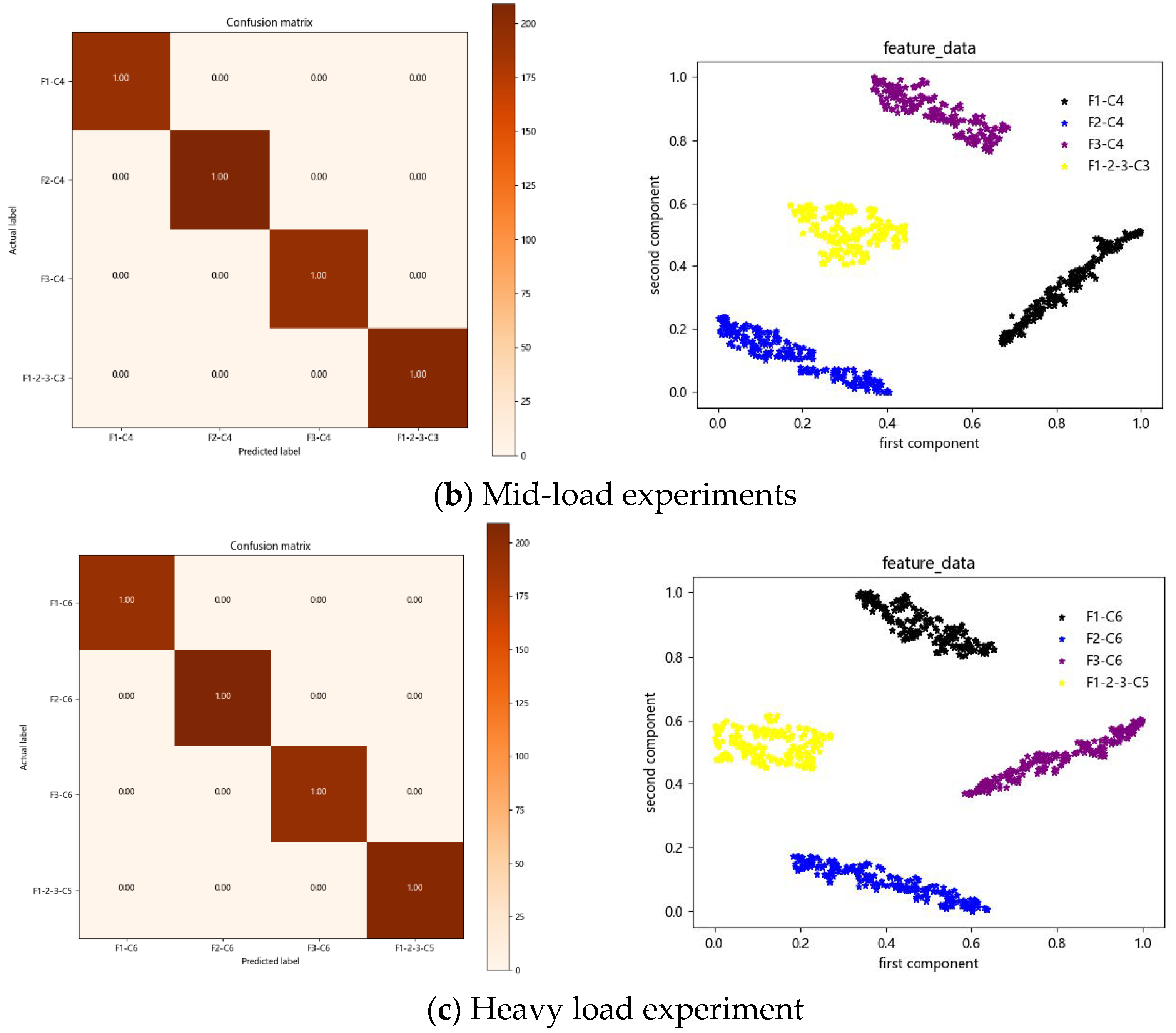
The comparison results of the first three sets of experiments are shown in
Figure 16. Through the confusion matrix and classification result graphs of the three sets of experiments, it can be seen that the FTF-DFD model proposed in this paper achieves the recognition of four types of position information, F1, F2, F3 and
, respectively, under light load, medium load and heavy load conditions, and all of them achieve 100% recognition accuracy.
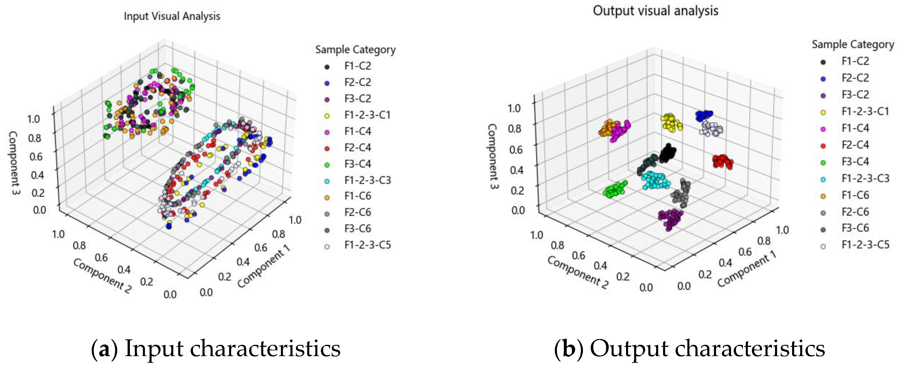
The fourth set of experiments took the 12 sets of work condition data involved in this paper and input them into the evaluation model after the data sample expansion of overlapping sampling, and the final output was divided into 12 clusters by t-SNE visualization. According to the input features in
Figure 17a, it can be seen that compared with the Western Reserve University 10 classification task features are completely mixed, the original input data of this experiment are mainly divided into two parts, F1 and F3 positions at all the working condition data are mixed together, and F2 is mixed with all the working condition data at position
, indicating that the original feature distributions of these data are closer and cannot be easily distinguished from each other. The classification result graph of the output of
Figure 17b shows that the experimental data of all kinds of working conditions of the model are improved from the chaotic state to the aggregated state, and the classification task of 12 working conditions is completed effectively, and all the working condition information is completely distinguished. The experiments are conducted by expanding different sample sizes, and it can be seen that the feature distributions in the two groups of working conditions, F2 (C2) and
(C5), are always closer, indicating the similarity of the feature components in these two groups of working conditions. This proves that the algorithm in this paper can effectively realize the working condition recognition under the uneven bearing load.


