Novel Process Modeling of Magnetic-Field Assisted Finishing (MAF) with Rheological Properties

Abstract

The performance of a magnetic-field-assisted finishing (MAF) process, an advanced surface finishing process, is severely affected by the rheological properties of an MAF brush. The yield stress and viscosity of the MAF brush, comprising iron particles and abrasives mixed in a liquid carrier medium, change depending on the brush’s constituents and the applied magnetic field, which in turn affect the material removal mechanism and the corresponding final surface roughness after the MAF. A series of experiments was conducted to delineate the effect of MAF processing conditions on the yield stress of the MAF brush. The experimental data were fitted into commonly used rheology models. The Herschel–Bulkley (HB) model was found to be the most suitable fit (lowest sum of square errors (SSE)) for the shear stress–shear rate data obtained from the rheology tests and used to calculate the yield stress of the MAF brush. Processing parameters, such as magnetic flux density, weight ratio of iron and abrasives, and abrasive (black ceramic in this study) size, with p-values of 0.031, 0.001 and 0.037, respectively, (each of them lower than the significance level of 0.05), were all found to be statistically significant parameters that affected the yield stress of the MAF brush. Yield stress increased with magnetic flux density and the weight ratio of iron to abrasives in MAF brush and decreased with abrasive size. A new process model, a rheology-integrated model (RM), was formulated using the yield stress data from HB model to determine the indentation depth of individual abrasives in the workpiece during the MAF process. The calculated indentation depth enabled us to predict the material removal rate (MRR) and the instantaneous surface roughness. The predicted MRR and surface roughness from the RM model were found to be a better fit with the experimental data than the pre-existing contact mechanics model (CMM) and wear model (WM) with a R² of 0.91 for RM as compared to 0.76 and 0.78 for CMM and WM. Finally, the RM, under parametric variations, showed that MRR increases and roughness decreases as magnetic flux density, rotational speed, weight ratio of iron to abrasive particles in MAF brush, and initial roughness increase, and abrasive size decreases.

1. Introduction

Magnetic-field assisted finishing (MAF) uses a flexible magnetorheological brush composed of iron and abrasive particles typically mixed in a liquid medium to yield a superfine surface quality. The flexible nature of the brush makes MAF one of the most suitable candidates for polishing complex geometries such as cylindrical [1] and freeform surfaces [2], cavities [3], and internal grooves [4]. With the development of metal additive manufacturing (AM) [5,6,7,8,9], which is capable of producing various complex designs and shapes that are not feasible with any conventional subtractive manufacturing, there has been an increasing demand for viable finishing technologies for complex AM-fabricated geometries. Although there are other advanced finishing processes that can improve the surface quality of the parts to a fine scale such as elastic emission machining (EEM) [10] and chemical–mechanical polishing (CMP) [11], thanks to the shape-adaptive flexible polishing brush, MAF has garnered much interest regarding the post processing of additively manufactured components [12,13,14]. The MAF process was implemented to polish various kinds of materials, such as mold steels [15], glass [16], ceramics [17], sheet metals [18], and titanium alloys [19].

Figure 1 shows the schematic of the MAF process in a computerized numerical control (CNC) milling setup, where the MAF brush is attached to a magnetic tool and the tool holder is generally rotated with the spindle. The workpiece is fixed with the carriage, which provides a linear motion. In the MAF brush shown in Figure 1, the abrasives are entrapped among the ferromagnetic chains that are aligned with the magnetic lines of force. The entrapped abrasives in contact with the workpiece are called active abrasives as they participate directly in the material removal process.

The key factors in the effective implementation of MAF are to understand the material removal mechanisms underlying the process and the effect of various processing parameters in order to find the optimum processing conditions [21,22,23]. As there are numerous processing parameters affecting the efficiency of the material removal process as well as the attainable final surface quality of the polished workpiece, relying purely on a series of experiments is extremely time-consuming. Hence, the development of an accurate process model to simulate and predict the material removal rate (MRR) and instantaneous surface roughness is important when determining the underlying material removal mechanisms and optimizing the MAF processing parameters.

It is extremely crucial to understand the nature of the material removal phenomenon to formulate a precise analytical model. Micro-cutting/chipping [24] and micro-ploughing [25,26] are reported to be the primary modes of material removal during the MAF. Several studies were carried out to formulate an appropriate model to study the material removal phenomenon and the effect of parametric variation in the MAF process [27,28,29,30,31,32,33]. One of the earliest works simulating surface accuracy in MAF was conducted by Kim et al. [32]. They used a wear model formulated by Rabinowicz [34] to predict wear in a three-body abrasion process. The material removal model was based on the micro-cutting phenomenon with the sharp cutting edges of conical abrasives. Since then, the wear model, relating the total material removal to the normal force and hardness of the work material, has been implemented by various researchers in the modeling of MAF [27,28,35]. Jayswal et al. [35] and Misra et al. [27] used a micro-cutting-based wear model with spherical abrasives. Misra et al. [27] also introduced a novel approach to decouple the total MRR into two parts: (a) steady-state MRR only affected by the processing conditions and (b) transient MRR depending on the remaining volume of irregularities on the surface at a given instantaneous time. This approach was based on the observation made by several researchers that MRR and surface roughness of the work material initially exponentially decrease but eventually saturate after some time [32,36,37]. Qian et al. [38] established the MRR in the MAF using Preston and Archard wear equations. Preston observed that MRR is proportionally related to the pressure acting on the workpiece surface and relative velocity between workpiece and brush for the lapping process on glass [39]. Similarly, Zhang et al. [40] modified the Archard equation considering a small portion of the contact area and calculated material removal in terms of depth and area. The Hertzian contact theory was used to calculate the maximum contact pressure and its distribution.

The material removal phenomenon in MAF depends on various processing conditions [26,27,41]. Jain et al. [41] studied the effect of several parameters on the final surface quality of the part and found that increasing the magnetic flux density, magnetic abrasive particles size, spindle speed, and volume fraction of iron particles resulted in a positive effect on improving final surface quality, whereas increasing the working gap proved to be detrimental. Similar results were reported by Misra et al. [27].

Although several researchers have studied various processing conditions and their effect on the MAF performance, there has not been a thorough understanding of how the rheological characteristics (for example, the yield strength) of the MAF brush affect the MAF performance. There have been studies on the rheological behavior of the lubricants on other similar finishing processes, such as CMP [42], but an in-depth analysis of the rheological properties of MAF is an understudied topic. The yield stress, determined by the strength of the iron particle chain (referred to as stiffness in this study) in an MAF brush under magnetic field [43], directly affects the MRR and the instantaneous change in surface roughness. The stiffness of the MAF brush dictates the intensity of the contact between abrasives in the MAF brush and the work surface. A stiff MAF brush holds the abrasive particles securely and promotes aggressive two-body abrasion, whereas a loose MAF brush promotes less aggressive three-body abrasion. The interesting results were reported by Sidpara et al. [43,44], who studied the effect of the rheological characteristics of the MAF brush on surface finishing quality in MAF. The changes in abrasive concentration, magnetic field, and liquid carrier concentration were found to vary the rheological properties of the MAF brush, such as viscosity and yield stress [44,45]. Sidpara et al. [43] observed that as the magnetic flux density and iron particle concentration increased, yield stress and viscosity increased as well, which in turn increased the MRR. The opposite trend was found with the abrasive volume concentration. This shows that the change in rheological properties changes the contact dynamics between the MAF brush and the workpiece and directly affects the material removal phenomenon in the MAF and the final surface quality of the polished parts.

Therefore, even though the rheological properties of the MAF brush are extremely vital parameters that directly affect the MRR in the MAF, their impacts have not been studied in depth. Sidpara et al. [43,44] studied the effect of various conditions on the rheological properties of the MAF brush and its subsequent effect on the surface quality of the finished parts experimentally. However, no process model has been developed to predict the MRR and surface roughness based on the rheological properties of the MAF brush. Therefore, the model presented in this study tries to fill this research gap and represents a major advance in understanding and predicting the MAF process. The results obtained from the model will be analyzed to understand the underlying material removal mechanism during MAF under various processing conditions. Finally, the effect of various processing parameters on the MRR and surface roughness will be predicted and analyzed using the developed model.

2. Materials and Methods

MAF Experimental Setup

MAF experiments were conducted on the CNC milling machine (VF4, HAAS, Los Angeles, CA, U.S.A.). A magnet holder was fabricated and used to hold multiple permanent magnets (Neodymium disc countersunk hole magnets, each a the diameter of 9 mm, a thickness of 5 mm, and a magnetic flux density of 120 mili-tesla (mT)), as shown in Figure 1. Magnetic flux density (B) was varied by changing the number of magnets held inside the magnet holder. The magnetic flux density of 120 mT was measured with a single magnet, whereas 180 mT and 220 mT were measured with two and three magnets in series, respectively. An MAF brush was attached onto the surface of the magnet. The magnet holder was assembled into the spindle, which allowed the brush to rotate and translate along the workpiece surface. A similar experimental setup was reported by the authors’ group on a previous study that assessed the effect of nano-scale solid lubricants on the MAF process [15].

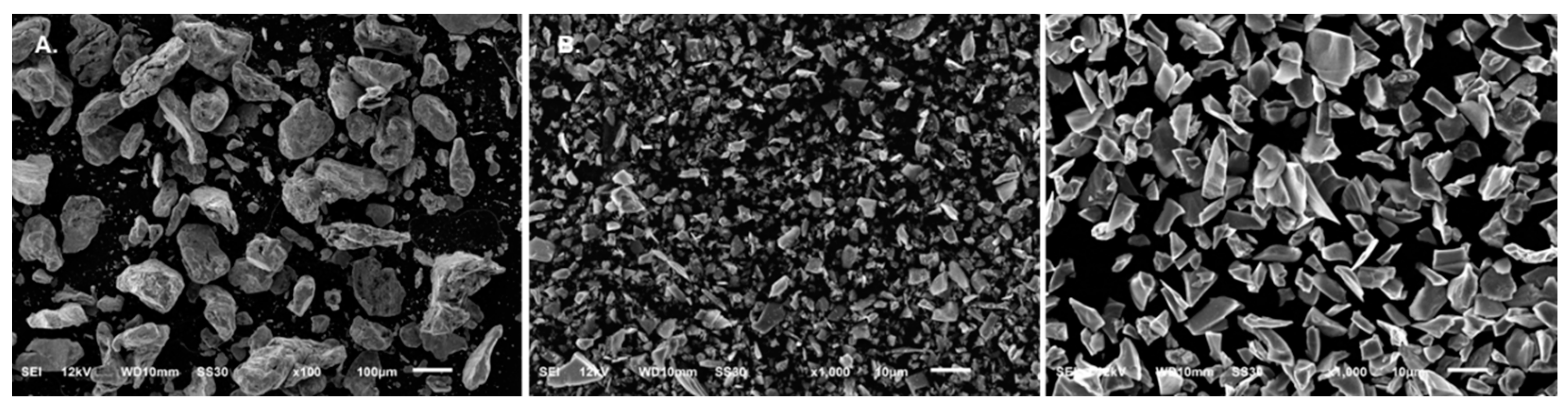
MAF Brush and Workpiece Materials

Black ceramic (BC) (Industrial Supply Inc., Baton Rouge, LA, USA), iron particles (the mean diameter of 300 μm, 40–60 mesh, Carolina Biological Supply Co., Burlington, NC, USA), and silicone oil (Xiameter PMX-200 Silicone Fluid 1,000,000 centistokes (cSt), The Dow Chemical Company, Midland, MI, USA) were the main constituents of the flexible MAF brush. The work material selected for this study was mold steel (CENA-V, Hitachi Materials, Japan). The work surface was milled to attain the average surface roughness, R_a, ranging from 1.5 to 6 µm. The SEM images of iron and black ceramic particles used in this study are presented in Figure 2.

Surface Characterization

Average surface roughness, R_a, is one of the most widely used parameters to characterize roughness. Hence, it was used as the parameter that characterizes roughness in this manuscript as well. R_a is defined as an average of the profile deviation from a mean line. The mean line (an imaginary line) divides the surface profile into two halves (peak half and valley half) so that the areas of both halves are equal. A stylus profilometer (Surfcom 50, Midwest Metrology, Holland, MI, USA) was used to measure the surface roughness. A diamond tip in the stylus profilometer senses or detects the deviation in the surface and provides the roughness measurement as it traverses in a line along the surface profile. An average of ten-line measurements is taken and reported as a roughness value throughout this study.

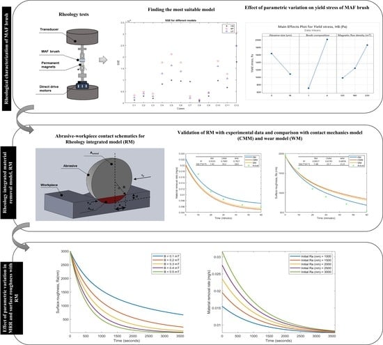
2.1. Rheology Tests

2.1.1. Design of Experiments

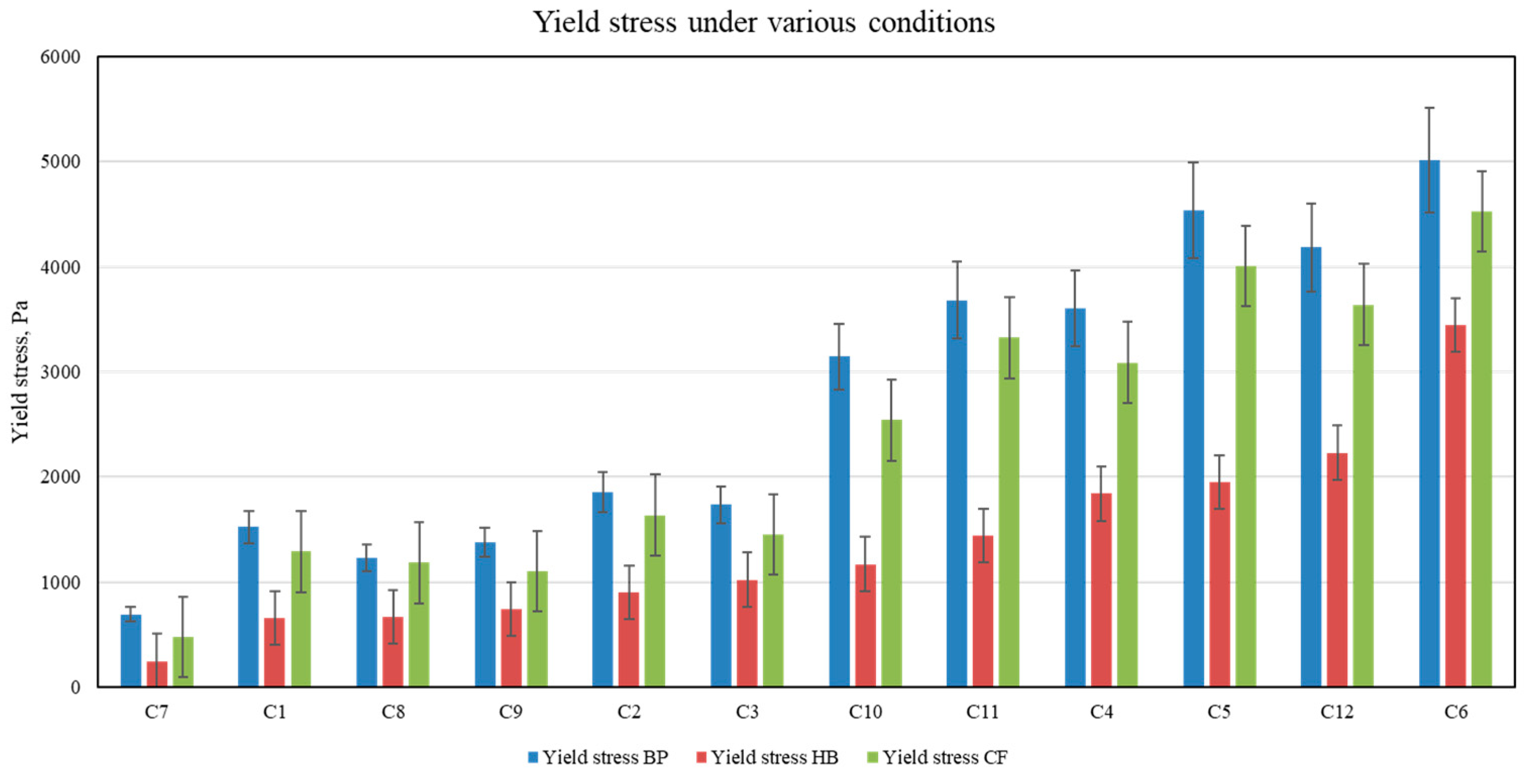
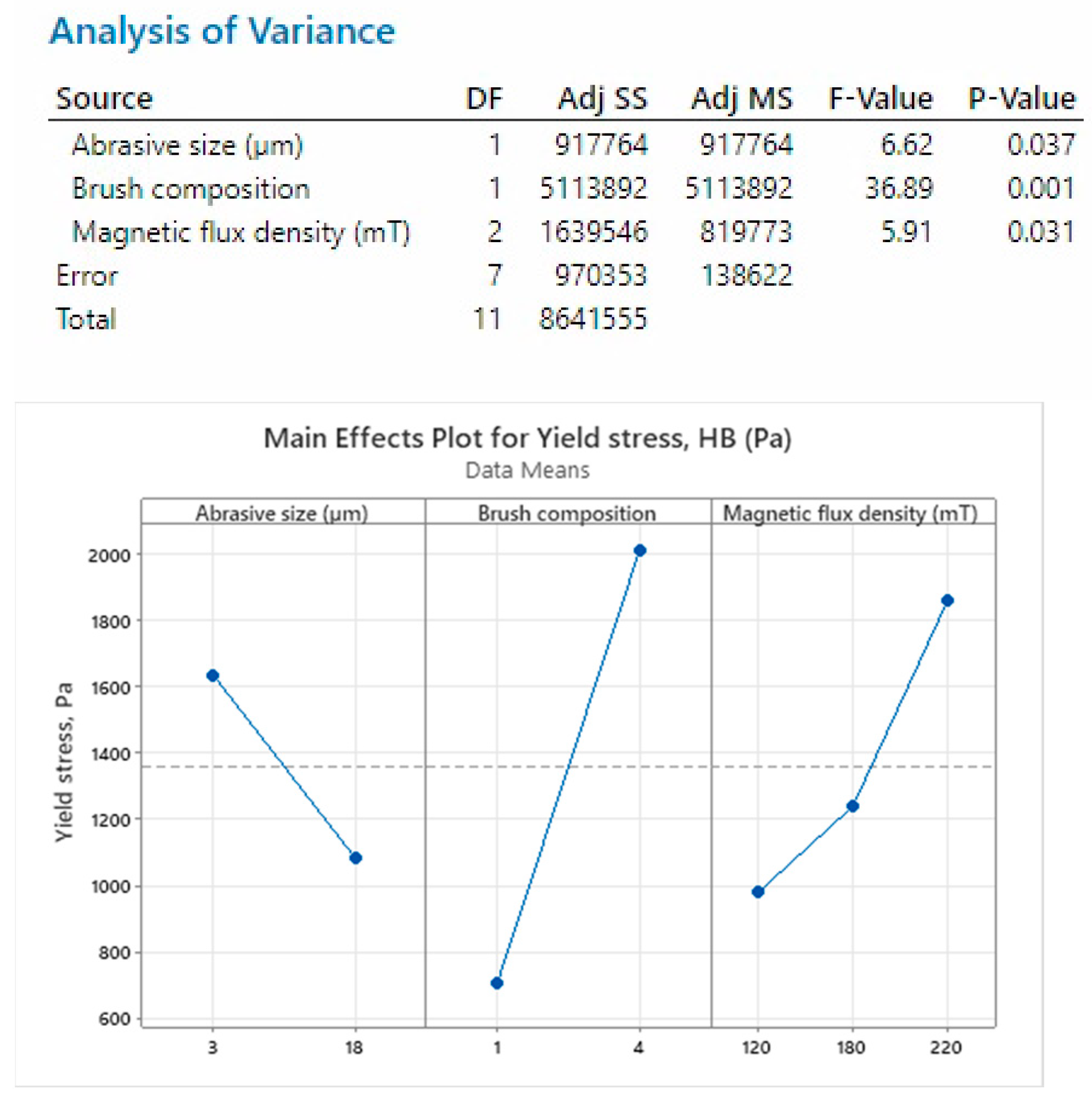
The primary parameters for the rheological properties of the brush were magnetic flux density, brush composition/iron-to-abrasive weight ratio (“Brush composition” terminology has been used to define the weight ratio of iron to abrasives in this manuscript), and abrasive particle size. The effect of these parameters on rheological characteristics can be studied with the flow shear rate ramp test, where the shear stress is recorded as a function of the shear rate. The change in shear stress with respect to shear rate is monitored and analyzed to calculate viscosity and yield stress. Twelve test cases, as shown in

Table 1. Design of experiments (DOE) to study the rheological parameters of various MAF brush conditions.

S.N.	Abrasive Size, D (µm)	Iron-to-Abrasive Weight Ratio	Magnetic Flux Density, B (mT)
C1	3	1:1	120
C2	3	1:1	180
C3	3	1:1	220
C4	3	4:1	120
C5	3	4:1	180
C6	3	4:1	220
C7	18	1:1	120
C8	18	1:1	180
C9	18	1:1	220
C10	18	4:1	120
C11	18	4:1	180
C12	18	4:1	220

, were conducted with the magnetic flux density varying at three levels (120, 180, and 220 mT), iron-to-abrasive weight ratio at two levels (1:1 and 4:1), and abrasive sizes at two levels (3 µm and 18 µm). All these experiments were repeated twice for a repeatability study of the data.

The cases are represented as Ci_(x,y,z), where I is the case number and the subscripts x, y and z represent abrasive size, iron-to-abrasive weight ratio and magnetic flux density, respectively, in the following sections of the manuscript. For example, case number 8, where experiments were conducted with 18 µm sized abrasives, 1:1 iron-to-abrasive weight ratio, and 180 mT magnetic flux density, will be represented as C8_(18,1:1,180).

2.1.2. Rheology Models

The most commonly used rheology models for viscoelastic fluids are Bingham plastic, Herschel–Bulkley, and Casson fluid model [44,45]. These models are represented in

Table 2. Various rheological models and their constitutive equations.

Model	Constitutive Equations
Bingham Plastic model	$\tau ={\tau }_y+\eta \dot{\gamma }$	(1)
Herschel–Bulkley model	$\tau ={\tau }_y+K{\dot{\gamma }}^n$	(2)
Casson fluid model	$\sqrt{\tau }=\sqrt{{\tau }_y}+\sqrt{{\eta }_{\inf }\dot{\gamma }}$	(3)

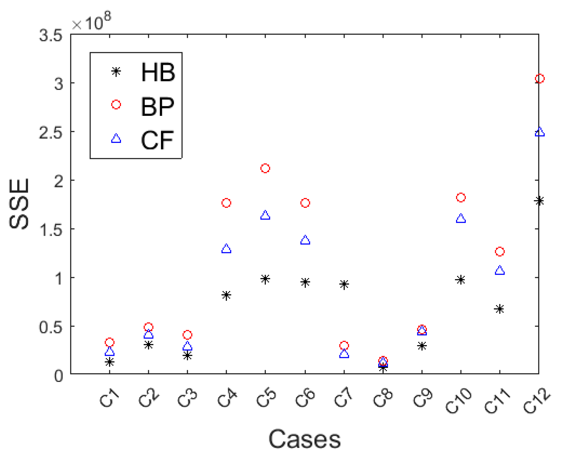
using viscosity ($\eta$), shear stress ($\tau$), yield stress (${\tau }_y$) and shear rate ($\dot{\gamma }$). $K$ and $n$ signify the consistency and power-law index, whereas ${\eta }_{\inf }$ represents suspension viscosity at an infinite shear rate. The suitability of these rheology models with the obtained rheological property data of an MR fluid was analyzed using statistical methods such as the least square sum of errors (SSE) method and R² method. SSE is the sum of square of residuals or deviations from the actual data to the predicted values from the analytical model. A lower SSE value means a better fit between the model and the experimental data. The R² value is the proportion of the variation in the dependent variable that is predictable from the independent variable(s). R² ranges from 0 to 1; the higher the R², the better the fit.

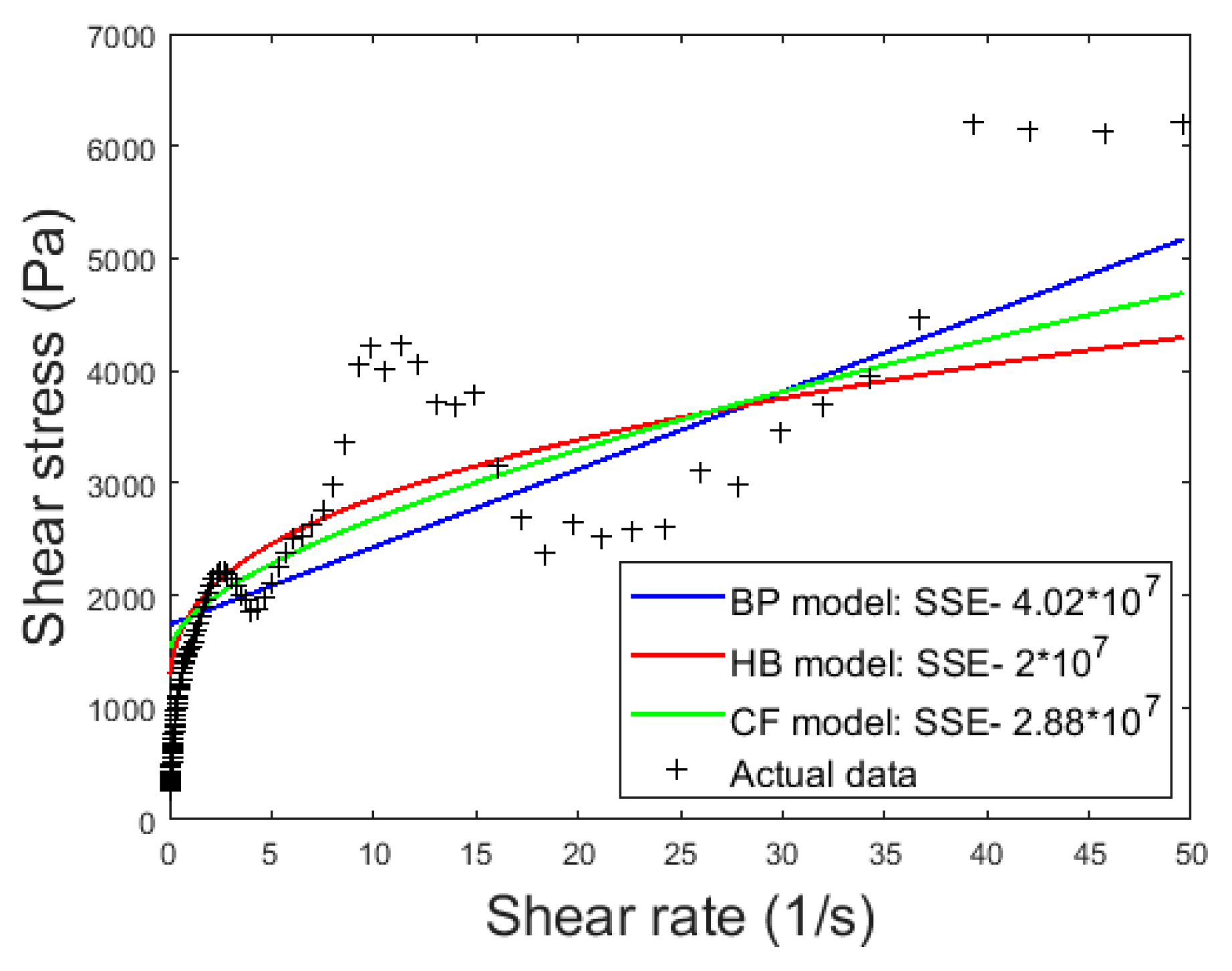
An the important parameter in characterizing the rheological property of magnetorheological fluid is yield stress. Materials act like a rigid solid under low stresses until reaching a certain level of stress, known as yield stress [46], after which they exhibit plastic deformation. The Bingham plastic (BP) model assumes that after the shear stress increases beyond yield stress, the material behaves as a Newtonian fluid, meaning the shear stress has a linear relationship with shear rate, described by a constant viscosity. However, viscosity increases with shear rate for some fluids (shear-thickening fluid) while it decreases for other fluids (shear thinning fluid). The Herschel–Bulkley (HB) model assumes a rigid pre-yield behavior, as occurs in the BP model. However, the HB model has the consistency index, $K$, with the power index, $n$, indicating whether the fluid is shear-thinning ($n$ < 1), shear thickening ($n$ > 1) or Newtonian ($n$ = 1) beyond the yield point. The Casson Fluid (CF) model is another widely used model to describe time-independent viscosity [40]. Continuous shear-thinning is assumed in the CF model, where viscosity decreases from infinity (at zero shear rate) to zero (at infinite shear rate).

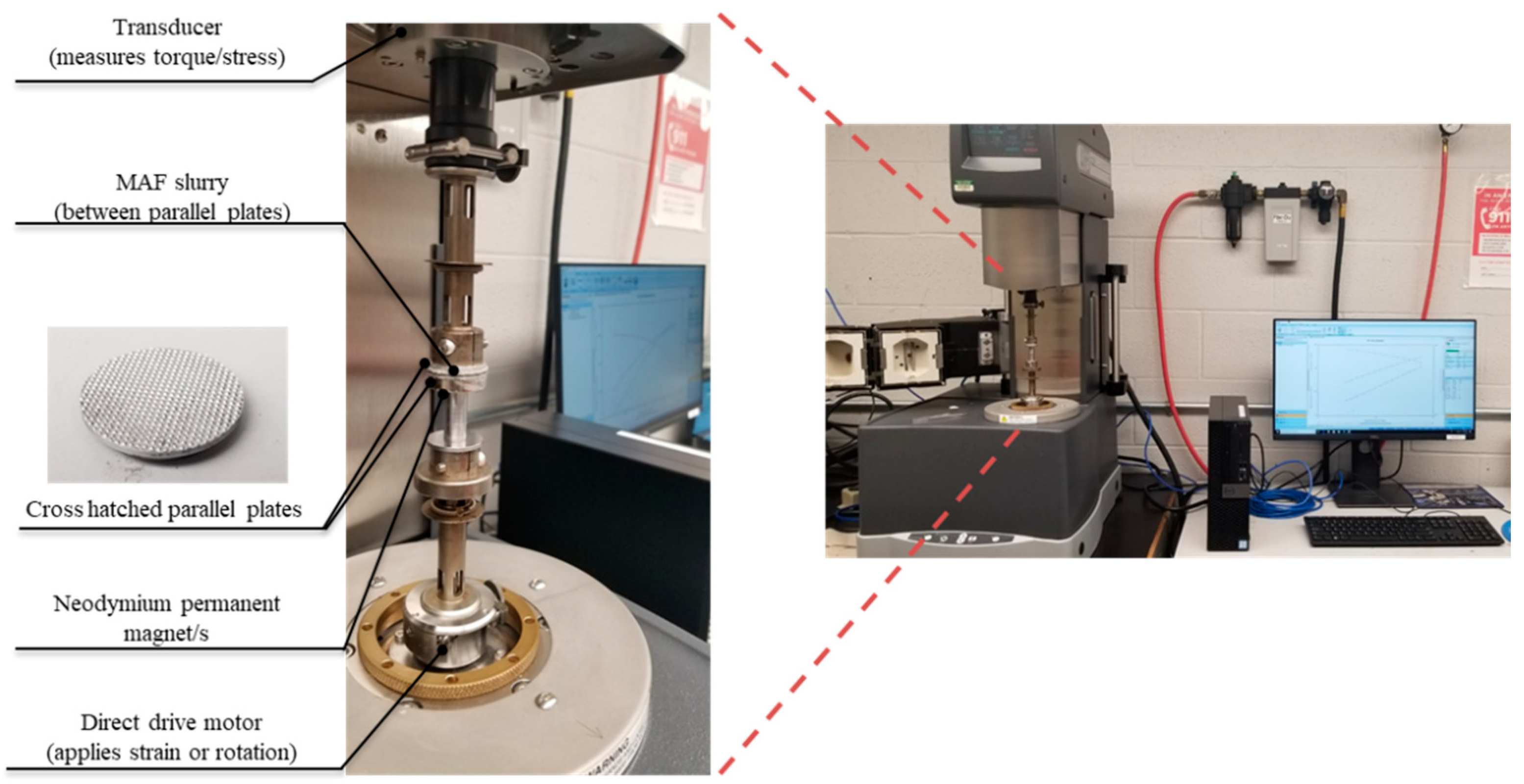
2.1.3. Rheology Test Equipment, Tests and Rheological Parameters

Rheology tests were conducted in an ARES-G2 rheometer (TA instruments, New Castle, DE, USA). Figure 3 shows the experimental setup. In order to incorporate the magnetic field, custom-made parallel plates were designed to attach permanent neodymium magnets beneath the parallel plates. The parallel plates that were used were machined to have a crosshatched pattern, as shown in Figure 3, to avoid the slippage issue that is common during higher shear rates. Continuous shear rate ramp tests were conducted under various conditions (as presented in Table 1) of the MAF brush to analyze the relationship between shear stress and shear rate and determine the yield stress for each condition. Due to the slippage issue at very high shear rates, the test was conducted while decreasing shear rate ramp from 50 1/s to 0.05 1/s.

2.2. Material Removal Model and Surface Roughness Model

2.2.1. Force and Number of Active Abrasives Calculation

For this preliminary study, even though the abrasives had an irregular shape, as seen in Figure 2, all the abrasives were assumed to be completely spherical in shape for simplification. Additionally, even though iron particles may also take part in the material removal process, because the iron particles have significantly lower hardness compared to abrasives, the abrasive effect of iron particles was assumed to be negligible in this study. For the material removal calculation, the number of active abrasives in contact with the workpiece was calculated based on the iron-to-abrasive weight ratio and the mass of each constituent used in the brush. 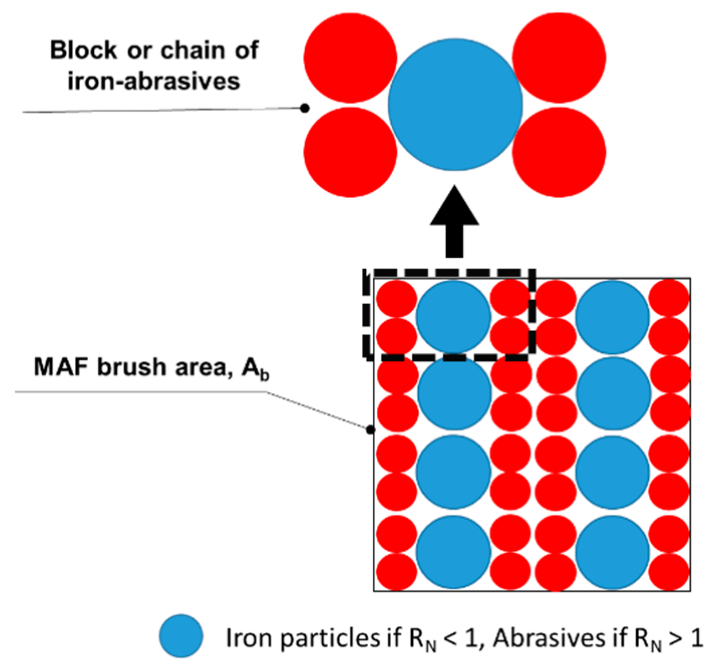Based on the volume and mass of the brush used for the MAF, the number of abrasives, iron particles, and volume fraction of each brush constituent could be found [15]. The number of active abrasives was then calculated in the following manner.

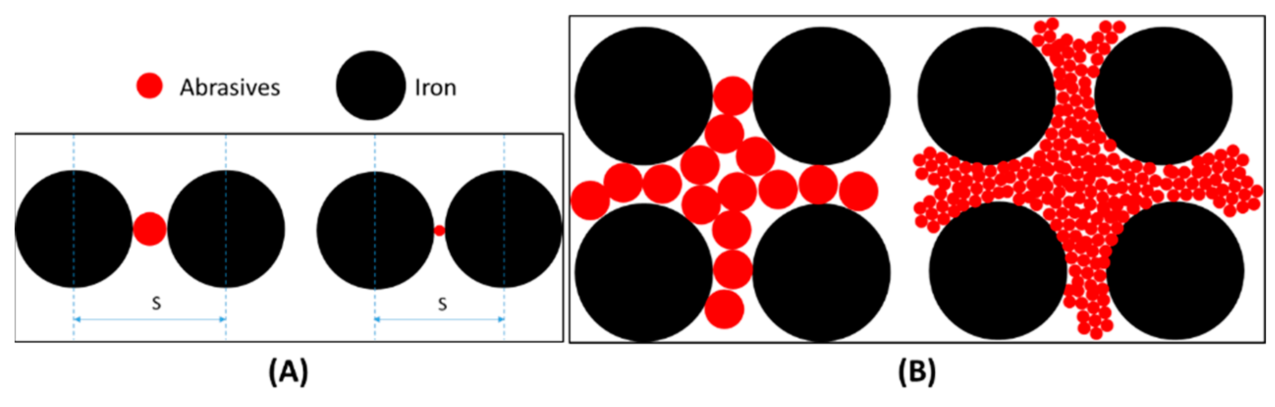
First, the ratio of the number of irons to abrasive particles, R_N, was calculated. Iron particles and abrasives arrange themselves in a block with a single particle surrounded by their counterparts, as shown in Figure 4 (depending on the content ratio between iron and abrasives), in the brush. Regardless of the iron-abrasive arrangement (the body center cubic arrangement shown in Figure 4), with the perfect packing, a block can have a different shape, but the area of the block would be the same. Hence, by calculating the number of iron and abrasives in each block, the area of each block was calculated. Finally, the area of a block (A_block) was then used to calculate the number of active abrasives.

$$Ratio of iron to abrasives, R_N=\frac{Number of iron particles}{Number of abrasives}$$

(4)

$$\begin{gathered} Area of each block, A_{block}=R_N\ast A_{one-abrasive}+A_{one-iron}, if R_N<1 \\ Area of each block, A_{block}=R_N\ast A_{one-iron}+A_{one-abrasive} ,if R_N>1 \end{gathered}$$

(5)

$$Number of blocks, N_b=\frac{Brush area, A_b}{A_{block}}$$

(6)

$$\begin{gathered} Number of active abrasives, N_{act}=N_b, if R_N>1 \\ Number of active abrasives, N_{act}=N_b\ast R_N, if R_N<1 \end{gathered}$$

(7)

Then, the normal force exerted by each abrasive on the workpiece surface was calculated using the following equations:

$$f_N=\frac{F_N}{N_{act}}=\frac{P_N\ast A_b}{N_{act}}$$

(8)

$$P_N=\frac{B_{avg}^2}{4\ast {\mathrm{\mu }}_0}\ast \frac{3\ast \mathsf{\pi }\ast \left({\mathrm{\mu }}_{FP}-1\right)\ast \alpha }{3\left(2+{\mathrm{\mu }}_{FP}\right)+\mathsf{\pi }\ast \left({\mathrm{\mu }}_{FP}-1\right)\ast \alpha }$$

(9)

where $F_N$ and $P_N$ are the normal force and pressure exerted over the MAF brush surface area, $A_b$. Average magnetic flux density is represented as $B_{avg}$, $N_{act}$ is the number of active abrasives, and $\alpha$ is the volume fraction of ferromagnetic particles in the MAF brush. The magnetic permeability in vacuum and relative magnetic permeability of ferromagnetic particles are denoted by ${\mathrm{\mu }}_0$ and ${\mathrm{\mu }}_{FP}$, respectively. The values of ${\mathrm{\mu }}_0$ and ${\mathrm{\mu }}_{FP}$ are 4π × 10⁻⁷ H/m and 5000 for 99.8% pure iron, respectively [15].

2.2.2. Calculation of Indentation Depth

Contact Mechanics Model (CMM)

Hertzian contact mechanics theory was used to determine the indentation depth in this model. Active abrasives in contact with the workpiece can be modeled as a rigid spherical indenter, whereas the workpiece can be taken as an elastic half-space. The indentation depth, calculated using the Hertzian contact mechanics method, is an elastic contact depth, which can potentially be abraded by an active abrasive on the workpiece. The normal force on each active abrasive under a given magnetic flux density can be calculated, which can be used to determine the indentation depth. Figure 5 shows the schematics of the spherical abrasive–workpiece contact, modeled as Hertzian contact, between the sphere and elastic half space.

$$\frac{1}{E^{\ast }}=\frac{1-{\nu }_1^2}{E_1}+\frac{1-{\nu }_2^2}{E_2}$$

(10)

$$f_N=\frac{4}{3}\ast E^{\ast }\ast R^{0.5}\ast d^{1.5}$$

(11)

$$a=\sqrt{R\ast d}$$

(12)

where $E$ and $\nu$ represent the Young’s modulus and Poisson’s ratio, respectively. $R$, $a$, and $d$ are the radius of a spherical abrasive particle, the contact radius, and indentation depth, respectively, as shown in Figure 5. Subscript 1 and 2 are used for the abrasive and workpiece, respectively, to define $E_1$ and $E_2$ and ${\nu }_1$ and ${\nu }_2$.

Wear Model (WM)

Rabinowicz et al. [34] introduced the concept of an analytical modeling of wear in the early 1960s based on the micro-cutting process. In this model, the indentation area is calculated by a simple wear equation, where the hardness of the workpiece material is the ratio of exerted normal force to the indented area of contact normal to the force [34]. Jain et al. [47] modified the wear equation, replacing the hardness with flow stress, since brittle materials show a different wear behavior than the ductile materials. Flow stress,${\sigma }_w$, was then related to Brinell hardness (BHN) by multiplying a constant, K. The value of K is 1 for brittle materials and greater than 1 for more ductile materials [47].

$${\sigma }_w=\frac{f_N}{Area of contact/indentation}=K.BHN$$

(13)

Using Equation (13), the area of indentation and indentation depth can be calculated.

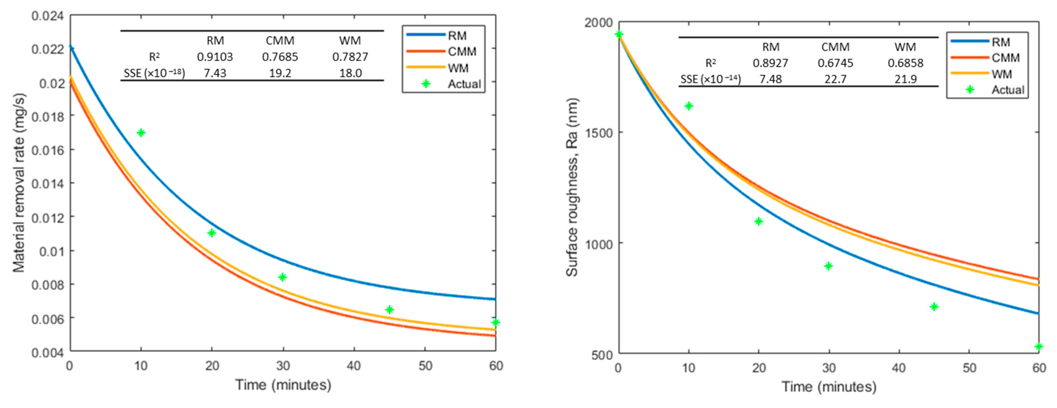
Proposed Rheology Integrated Model (RM)

Even though analytical models such as the contact mechanics and wear models presented above are already used to model MAF in the literature, a new method is introduced to calculate the indentation depth in the MAF in this paper. This is necessary as the contact mechanics model can only precisely predict indentation depth under the assumption of elastic deformation. However, the important process in the removal of material during MAF occurs during plastic deformation [48]. Wang and Wang mentioned that the plastic indentation depth is usually higher than the elastic indentation depth, which must be accounted for when calculating total wear volume [49]. Furthermore, the wear model only takes workpiece properties into account, ignoring the properties of the indenter, which is critical when attempting to understand the aggressiveness or degree of contact that affects the material removal mechanism. Hence, a new model must address the issues of the pre-existing models.

Wang and Wang [49] also noted that much of the wear debris does not appear as “chips” in MAF, which is normally seen in a cutting or micro-cutting process. MAF predominantly acts as a three-body abrasion process, which is mostly incorporated with the rolling phenomena of free abrasives, which usually cause micro-ploughing with plastic deformation [25,50]. Hence, the force equation used to calculate the amount of shear or tangential force required to plastically deform irregularities (which contributes to roughness) of the workpiece must be determined. To do so, the rheological property of the brush must be integrated to calculate the tangential force exerted by the abrasives during the MAF process. Several researchers have noted that the shear force applied during MAF by the abrasive should be higher than the resistance force (given by the yield strength of the workpiece material, $Y_w$) [35,51] to remove any workpiece material. 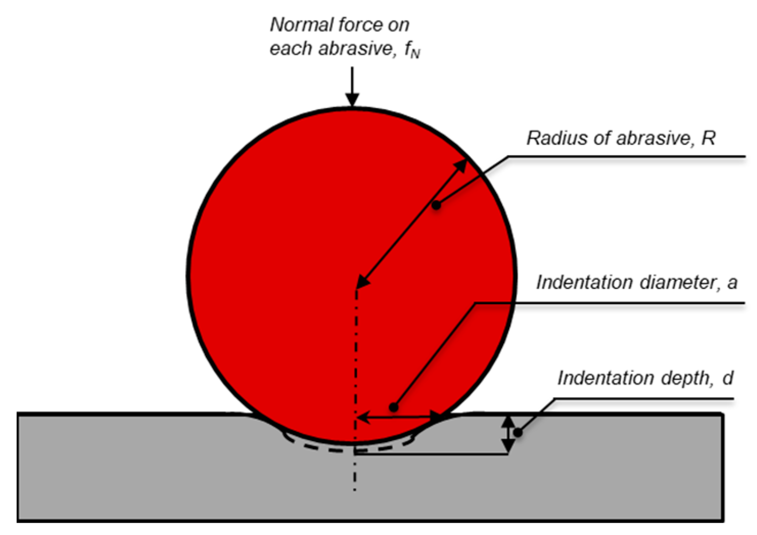The shear force acting in the MAF is dictated by the strengths of the iron-abrasive chains, which are governed by the yield stress of the MAF brush [43]. The maximum shear force that the MAF brush can exert in the workpiece surface is equal to the yield stress. Thus, a mathematical relation was devised to calculate the indentation depth of an abrasive on the workpiece material.

$${\tau }_y\ast A_{unind}=Y_w\ast A_{ind}$$

(14)

$${\tau }_y\ast \left(\mathsf{\pi }{R}^2-A_{ind}\right)=Y_w\ast A_{ind}$$

(15)

$$\frac{{\tau }_y}{{\tau }_y+Y_w}\left(\mathsf{\pi }{R}^2\right)=A_{ind}$$

(16)

where $Y_w$ is the yield strength of the workpiece, ${\tau }_y$ is the yield stress of the MAF brush, R is the radius of the abrasive, and $A_{ind}$ and $A_{unind}$ are the indented and un-indented areas of the abrasive, respectively, as shown in Figure 6. The indented area (area of chord in red, as shown in Figure 6) was used to calculate the indented area of an abrasive. Using Equation (18), the indentation depth, d, is calculated.

$$A_{ind}=\frac{R^2}{2}\left(\mathsf{\Theta }-Sin\mathsf{\Theta }\right)$$

(17)

$$A_{ind}=R^{2}Si{n}^{-1}\left(\frac{\sqrt{2Rd-d^2}}{R}\right)-\sqrt{2Rd-d^2}\ast \left(R-d\right)$$

(18)

The indentation depth was calculated, taking both the rheological properties of the MAF brush and the resistance properties of workpiece beyond the elastic contact region, which addresses the issues of both pre-existing models, WM and CMM.

2.2.3. Calculation of Material Removal Rate (MRR)

As mentioned before, some of the literature mentioned a high MRR at the initial phases of MAF, but this declines and eventually saturates over time [27]. This phenomenon occurs because of the rough initial surface. As the MAF process continues, the roughness and, consequently, the volume of irregularities decrease, causing the MRR to decrease as well. This observation led Misra et al. [27] to decompose the MRR into steady-state and transient components. This paper follows the same approach.

Steady-State MRR

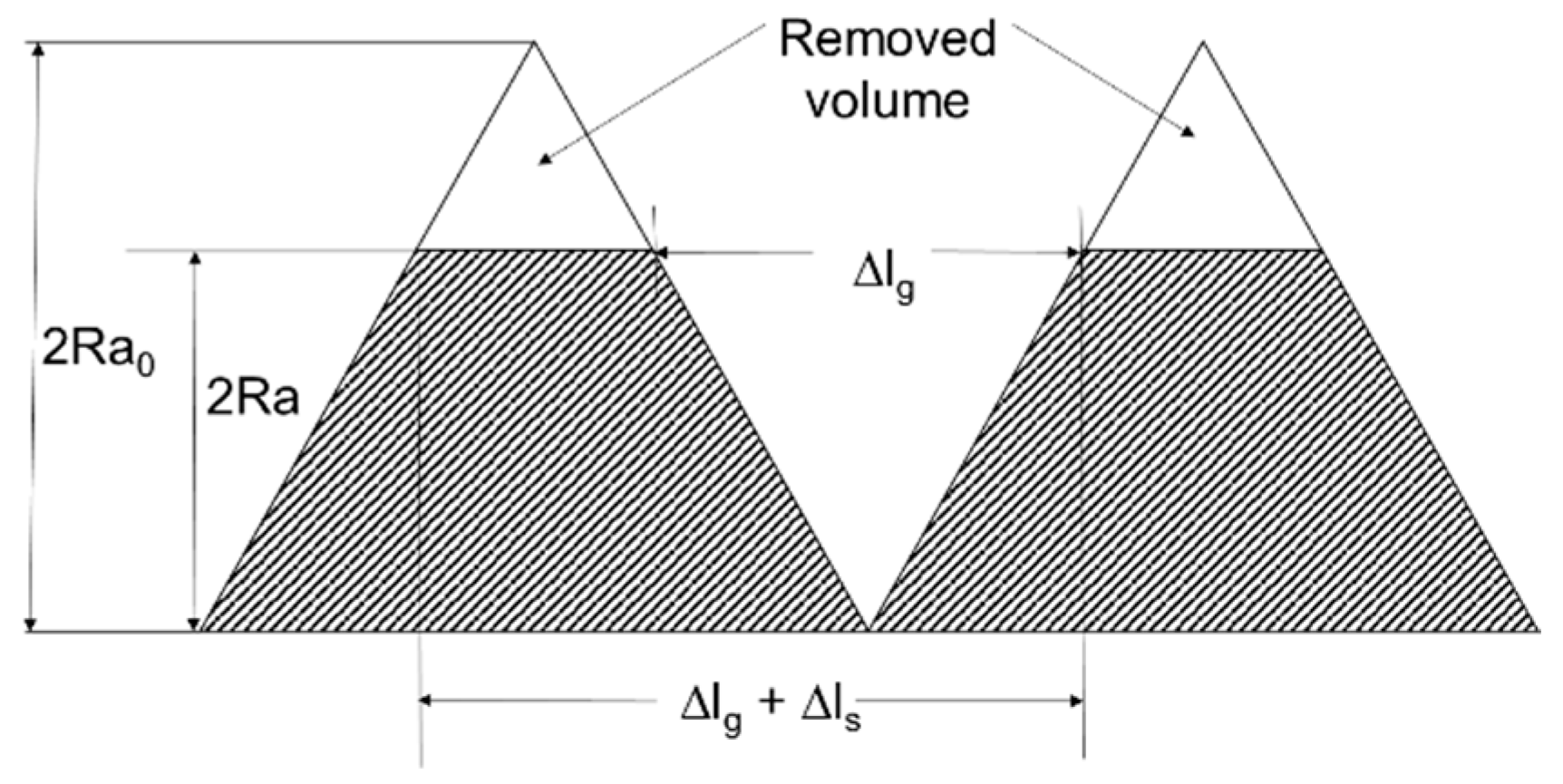
This component of MRR does not depend on time but entirely on MAF parameters. According to Preston [39], the MRR of MAF depends on the applied pressure (normal force divided by area of contact) and the average velocity of the abrasives. A modified equation for steady-state MRR developed by Misra et al. [27] mentioned that the total volume of irregularities removed by each abrasive during the steady state can be obtained by multiplying the indented contact area with the length travelled by the abrasives. Total length travelled, however, cannot be directly calculated by multiplying velocity and time, as the cross-section is not uniform. Kim et al. [32] mentioned that, with the triangular irregularities presented in Figure 7, the actual contact length is given by

$$l=\frac{∆l_s}{∆l_s+∆l_g}vt=\left(1-\frac{R_a}{R_{a0}}\right)vt$$

(19)

where $∆l_g$ represents the gap between two peaks, as shown in Figure 7, and $∆l_s$ represents the length of triangular base of the volume removed during MAF. $v$ is the average velocity, $R_{a0}$ is an initial surface roughness, and $R_a$ is the instantaneous roughness at time, $t$.

The irregularity volume removed by the active abrasives is

$$V_{irr}=N_{act}{K}_s{A}_{ind}vt\left(1-\frac{R_a}{R_{a0}}\right)$$

(20)

$${TMR}_s=V_{irr}\ast {\rho }_w$$

(21)

$$MR{R}_s=N_{act}{\rho }_w{K}_s{A}_{ind}v\left(1-\frac{R_{asteady}}{R_{a0}}\right)$$

(22)

where $MR{R}_s$ and ${TMR}_s$ are the steady-state MRR and the total material removed. $N_{act}$ is the number of active abrasives, ${\rho }_w$ is the workpiece density, $A_{ind}$ is the indentation area, and $K_s$ is a dimensionless constant that represents the probability of abrasives being in contact with the workpiece material. $R_{asteady}$ is the saturated surface roughness, the roughness value after a certain period when roughness saturates and does not decrease significantly over time.

Transient MRR

MRR depends hugely on the instantaneous irregularity volume that can be removed at a given instant [27]. If the irregularity volume available to be removed is high, abrasives can cut through more peaks and remove more material. Hence, Misra et al. [27] developed the relation

$$\frac{{dV}_{ins}}{dt}\alpha V_{iirr}\to \frac{{dV}_{ins}}{dt}=-C_T{V}_{iirr}$$

(23)

$${\int }_{V_0}^{V_{irr}}\frac{{dV}_{ins}}{V_{iirr}}={\int }_0^t-C_{T}tdt$$

(24)

$$V_{iirr}=V_0{e}^{-C_{T}t}$$

(25)

$$V_{ins}=V_0-V_{iirr}=V_0(1-e^{-C_{T}t})$$

(26)

where, $V_{ins}$ is the transient volume removed after time, t, $V_{iirr}$ is the instantaneous volume of irregularities left in the workpiece, $V_0$ is the initial irregularities volume, and $C_T$ is a transient MRR coefficient.

Assuming the triangular irregularities on the workpiece, initial volume of irregularities, $V_0,$ can be calculated in terms of initial surface roughness using simple mathematical relations. Misra et al. [24] found this relation to be

$$V_0=\frac{h{A}_f}{2}$$

(27)

where $h$ is the total height of peak to valley and $A_f$ is the area being finished during MAF.

Since the average roughness, $R_a$, is the average of profile deviations ($z$) from mean line, a relation between total depth between peak to valley, $h$, and $R_a$, over a sampling length, $l$, can be devised. Profile deviation (z) is calculated along the x-axis line where dx represents a small increment in x direction in a surface profile (for the assumed triangular irregularities, z can be represented as a function of x).

$$R_a=\frac{1}{l}{\int }_0^l\left|z\right|dx=\frac{h}{4}$$

(28)

From Equations (27) and (28), initial irregularity volume can be calculated as

$$V_0=2R_a{A}_f$$

(29)

The transient volume removal ($V_{ins})$, transient total material removed (${TMR}_{ins}$), and transient material removal rate (${MRR}_{ins}$) after time, t, are given by

$$V_{ins}=2R_a{A}_f(1-e^{-C_{T}t})$$

(30)

$${TMR}_{ins}=2{{\rho }_{w}R}_a{A}_f(1-e^{-C_{T}t})$$

(31)

$${MRR}_{ins}=2{{\rho }_{w}R}_a{A}_f{C}_T{e}^{-C_{T}t}$$

(32)

Hence, the total material removal rate is the summation of the steady state and transient material removal rate.

$${MRR}_{total}=MR{R}_s+MR{R}_{ins}$$

(33)

2.2.4. Calculation of Instantaneous Surface Roughness

Surface roughness follows a similar trend to MRR, which decays exponentially, and finally the surface roughness reaches the saturation stage. This trend of exponential decay led researchers to assume that the rate of change in surface roughness primarily depends on two important factors [28]: (1) instantaneous material removal rate, MRR, and (2) instantaneous surface roughness. Mathematically,

$$\frac{{dRa}_{ins}}{dt}\alpha (MR{R}_{total}{andR}_{ains})\to \frac{{dRa}_{ins}}{dt}=-C_{Ra}MR{R}_{total}{R}_{ains}$$

(34)

$$\frac{{dRa}_{ins}}{dt}=-C_{Ra}{R}_{ins}[N_{act}{\rho }_w{K}_s{A}_{ind}v\left(1-\frac{R_{asteady}}{R_{a0}}\right)+2{{\rho }_{w}R}_a{A}_f{C}_T{e}^{-C_{T}t}]$$

(35)

where ${Ra}_{ins}$ is the instantaneous surface roughness and $C_{Ra}$ is the coefficient of roughness.

Applying initial conditions, the equation reduces to

$${\int }_{R_0}^{R_{ains}}\frac{{dRa}_{ins}}{R_{ins}}={\int }_0^t\{-C_{Ra}\left[N_{act}{\rho }_w{K}_s{A}_{ind}v\left(1-\frac{R_{asteady}}{R_{a0}}\right)+2{{\rho }_{w}R}_a{A}_f{C}_T{e}^{-C_{T}t}\right]\}dt$$

(36)

$$R_{ains}=R_{a0}{e}^{[-C_{Ra}MR{R}_{s}t+2R_{a0}{A}_f{\rho }_w\left(1-e^{-C_{T}t}\right)]}$$

(37)

3. Results and Discussion

3.1. Rheology Test Results

3.1.1. Selection of Best Rheological Model

The flow shear rate ramp tests mentioned in Section 2.1.3 were conducted on an MAF brush under various conditions, as presented in Table 1. This test is used to relate shear stress with shear rate. Using the shear stress–shear rate data, the yield stress, ${\tau }_y$, of an MAF brush under the given conditions was determined using a non-linear, least square, regression curve fitting toolbox in MATLAB. Figure 8 shows the fluid models used and the fitness of each model using the estimated SSE values.

As shown in Figure 8, the HB model has the lowest SSE values in almost every case (except for one case, C7_(18,1:1,120)) indicating a better fit with the experimental data. Figure 9 shows a comparison of different models with actual data for case C3_(3,1:1,220).

However, an issue was encountered where almost every case in HB model yielded negative yield stress, as found by other researchers [52,53], which is physically meaningless. Kelessidis et al. [54] proposed a new golden section (GS) method to calculate the HB model parameters to avoid meaningless negative yield stress. Rooki et al. [55] also mentioned that standard statistical techniques may sometimes provide physically unacceptable solutions when using the HB model. Hence, a genetic algorithm (GA) was introduced to optimize and generate a reasonable set of optimized solutions in these cases [55,56]. GA is a technique for multi-objective optimization. Rooki et al. [55] also noted that the GA method was able to find a near-optimal solution with a lower SSE than other methods, such as power law and even the GS method [54].

Table 3. Comparison of HB parameters fitted using various statistical methods for case C3_(3,1:1,220).

Method	${\mathit{\tau }}_{\mathit{y}}$	$\mathbf{K}$	$\mathbf{n}$	SSE	R2
NL	−2764	4307	0.1247	2.02 × 107	0.861
NLP	0.00000154	1439	0.3011	2.324 × 107	0.8405
GA	1023.3	802.81	0.3599	2.08 × 107	0.7612

shows a particular case, C3_(3,1:1,220), with the HB model with various curve fitting methods. The SSE method and the coefficient of determination (R²) method were studied to determine their fitness. The non-linear (NL) regression method produced the lowest SSE and the highest R² result but generated a negative yield stress value. To avoid a negative yield stress, the constrains ${\tau }_y\ge 0, \mathrm{K}\ge 0, \mathrm{and} \mathrm{n}\ge 0$ were introduced and the parameters were calculated again. This method, named the non-linear regression method with penalty (NLP), was similarly used by Kelessidis et al. [54], and generated zero yield stress. This means that the HB model reduces to a power law model, which gives zero yield stress. Hence, this model was not suited to our case. Similarly, the power law model was noted to be unsuitable in many cases as it might not yield an optimal solution [55]. The GA method, however, provided an optimal solution with a reasonable value for yield stress. Moreover, even though the R² value resulting from the NLP method was higher than the GA method, the SSE value was lower for the GA method. Similar results were obtained by Rooki et al. [55].

Hence, the GA technique was used to fit the rheological experimental data (shear stress and shear rate) to an HB model and predict the HB model parameters: yield stress (${\tau }_y$), consistency index (K), and power law index (n). In the GA method, the SSE was used as an objective function subject to the conditions: ${\tau }_y\ge 0, \mathrm{K}\ge 0 \mathrm{and} \mathrm{n}\ge 0$.

$$SSE={\sum }_1^N{{(\tau }_i-{\widehat{\tau }}_i)}^2$$

(38)

where ${\tau }_i$ is the shear stress obtained experimentally, whereas ${\widehat{\tau }}_i$ is the shear stress obtained using the HB model equation (Equation (2)) for any set of yield stress, K and n. $N$ is the number of samples.

3.1.2. Effect of Processing Conditions on Yield Stress

Each test condition in Table 1 resulted in a distinct yield stress value. Comparisons of the yield stress values that were generated are presented in Figure 10. The cases are presented in ascending order with respect to yield stress. As shown in Figure 10, the highest yield stress was obtained under C6_(3,4:1,220) conditions, whereas the lowest yield stress was obtained for C7_(18,1:1,120) test conditions. The general linear model ANOVA (performed with 95% confidence interval on the yield stress data obtained using the HB model under different conditions) showed that all the studied parameters (abrasive size, brush composition/iron-to-abrasive weight ratio, and magnetic flux density) were statistically significant (p < 0.05), as shown in Figure 11 (top).

Ignoring the term with a third-level interaction between the analyzed three parameters, the regression equation was:

Yieldstress, HB = −121 + 2.86 magnetic flux density + 9.9 abrasive size + 78 brush composition − 0.113 magnetic flux density∗abrasive size + 2.72 magnetic flux density∗brush composition − 10.85 abrasive size∗brush composition

(39)

Among the various parameters, the brush composition/iron-to-abrasive weight ratio was found to be the most dominant factor (p = 0.001), followed by abrasive size and magnetic flux density. Figure 11 (bottom) shows the brush composition and magnetic field effect with positive slopes and the abrasive size with a negative slope. A positive slope indicates that the yield stress increases as the parameter is increased, whereas a negative slope means the opposite. Hence, a higher value of abrasive size and magnetic flux density yielded a higher yield stress, whereas larger abrasives decreased the yield stress.

The positive effect of magnetic flux density was observed by other researchers [43,44]. As the magnetic flux density increases, iron particles are held together with a stronger magnetic force, resulting in a stiffer MAF brush with a larger yield stress. The effect of the iron-to-abrasive weight ratio can be explained by calculating the volumetric composition in the MAF brush. Based on a 25 mm circular parallel plate with a 1 mm gap, the volume fraction of each brush constituent (iron, abrasives or silicone oil) was calculated and presented in

Table 4. Total mass, volume and volume fraction of MAF brush constituents for different brush compositions.

Constituents	Weight Ratio (Miron: Mabrasive) −1 to 1		Weight Ratio (Miron: Mabrasive) −4 to 1
	Mass (g)	Volume, mm3 (Volume %)	Mass (g)	Volume, mm3 (Volume %)
Iron	0.4902	51.9 (~10.57%)	1.2422	157.77 (~32.14%)
Abrasive	0.4902	132 (~26.89%)	0.31056	100.177 (~20.37%)
Silicone oil	0.6138	306.9 (~62.5%)	0.4658	232.91 (~47.4%)

. As is evident from Table 4, the volume fraction of iron particles increases with a higher iron-to-abrasive weight ratio. Sidpara et al. [44] reported a linear relation between yield stress and the particle volume fraction of the iron particles, which generate a stronger magnetic force in the MAF brush. Hence, yield stress was increased with an increase in the weight ratio of iron particles to abrasives.

The effect of the abrasive size can be explained by on the inter-particle distance between two ferromagnetic particles. With the increase in the abrasive size, the inter-particle distance between two ferromagnetic particles increases, as shown in Figure 12A. Huang et al. [57] noted an inverse relationship between the magnetic interaction force and particle distance. With the increase in the inter-particle distance, the decrement in magnetic interaction force results in a lower strength iron chain, and a low yield stress and viscosity in magneto-rheological fluid. Similar results were obtained by Nagdeve et al. [58].

However, it should be noted here that, with smaller particles, as seen in Figure 12B, the number of abrasives is higher. Therefore, there may not only be a single particle between two iron particles and the inter-particle iron distance may be unaffected, regardless of abrasive size. Another factor also plays a part in this discussion. With the smaller abrasives, the surface area of abrasives is much larger. In this case, as shown in Figure 12B, the interstitial spaces are smaller. Liquid silicone oil occupies these interstitial spaces, and, thus, they are lesser in amount with smaller abrasives. Sidpara et al. [44] noted that, with a lower concentration of carrier fluid, the yield stress increases. Hence, for these two reasons, smaller abrasives containing the MAF brush are stiffer, with higher yield stress.

Figure 13 shows the interaction plot between various variables regarding yield stress. The combination of higher magnetic flux–lower abrasive size, lower abrasive size–higher brush composition, and higher brush composition–higher flux density results in a higher yield stress.

4. Material Removal Model Test Results

4.1. Calculation of MRR and R_a

Using the procedure mentioned in Section 2.2, the normal force, number of active abrasives, and indentation depth were calculated using various numerical models, which determines the MRR and surface roughness for different test conditions. The constants (K_s, C_T, and C_Ra) were calculated for all the models for a specific case, C9_(18,1:1,220), by fitting the numerical models with the experimental results. The experimental data of the total material removed (TMR), MRR, and the instantaneous roughness for C9_(18,1:1,220) are presented in

Table 5. Material removal rate (MRR), total material removed (TMR) and surface roughness, R_a at different time before and during MAF.

Time (min)	TMR (mg)	MRR (mg/s)	Roughness, Ra (µm)
0	0	0	1.5782
10	6.3000	0.0105	1.2510
20	10.6000	0.0072	1.1580
30	13.7000	0.0052	1.0192
45	17.1000	0.0038	0.9460
60	19.4000	0.0026	0.9005
75	21.7000	0.0026	0.8858

.

Figure 14 shows a comparison between the experimental and predicted MRR, as well as surface roughness. The model provides an extremely good fit with the experimental results, with an R² up to 0.96 and 0.95 for MRR and surface roughness, respectively, which validates the model. Similarly, the constants in the MRR and roughness equations for RM were calculated and presented in Figure 14, and were used to predict and validate results for other MAF cases, as summarized in

Table 6. Experimental conditions used to perform MAF.

Experimental Conditions
RPM	2000
Brush diameter	18 mm
Clearance	1 mm
Magnetic flux density	120 or 180 or 220 mT
Abrasive diameter	3 or 18 µm
Length of the workpiece	30 mm
Brinell Hardness of Cena V steel	375
Ductility factor for steel, K	3 [27]
Density of black ceramic abrasives	3210 kg/m3
Density of iron particles	7874 kg/m3
Density of workpiece	7850 kg/m3
Young’s modulus of workpiece	208 GPa
Poisson’s ratio of workpiece	0.303
Young’s modulus of black ceramic abrasives	410 GPa
Poisson’s ratio of black ceramic abrasives	0.14

.

4.2. Validation of MRR and Ra with Another Condition and Comparison of Various Models

The constants calculated for C9_(18,1:1,220) for all three models were used to predict the MRR and R_a for case C10_(18,4:1,120). The predicted result was then compared with the experimental data. Figure 15 compares the actual and simulated data for all the indentation models. As observed from Figure 15, the results obtained from the RM showed a better fit than those from the WM and CMM. Based on R² and the SSE comparison among various models, R² was the highest and SSE was the lowest in terms of RM for both MRR and surface roughness data. RM showed a better fit than CMM because RM calculates the indentation depth and wear area assuming plastic deformation, whereas CMM only provides an indentation depth up to the elastic region. With the contact between the MAF brush and workpiece exceeding the elastic region in MAF, the indentation volume is more accurately predicted by the RM than the CMM method. Gao et al. [26] also reported that the CMM cannot accurately predict the indentation depth of abrasives in MAF by only considering elastic contact when calculating the indentation depth.

Similarly, the superiority of RM compared to WM can be accounted for by WM’s inability to incorporate the properties of the indenter or the MAF brush into the model. WM relates the area of indentation to normal force and workpiece hardness. The property of the indenter or the MAF brush is crucial to understand the aggressiveness of the abrasion or contact that directly affects the indentation depth and, subsequently, the material removal mechanism, which WM fails to take into consideration. However, RM incorporates not only the resistance property of the workpiece but also the rheological properties of the MAF brush. Hence, better predictions were made with RM than WM.

4.3. Parametric Variation Results after Simulation

The MAF process is affected by various processing parameters. Spindle speed, abrasive size, iron-to-abrasive weight ratio, initial surface roughness, and magnetic flux density are some of the major parameters affecting the performance of MAF. Using the constants obtained from Section 4.1 while keeping the other experimental conditions the same, the effect of various processing parameters on the MRR and surface roughness was studied and presented in Figure 16.

Most of the results generated from the model are in agreement with the previous works [22,27,59], which strengthens the validity of the model. The higher spindle speed increases the MRR due to the higher shear cutting force that occurs with high speed. This, in turn, decreases the final surface roughness, as shown in Figure 16a. Similarly, as the magnetic flux density increases, TMR increases (Figure 16b) as well. As discussed in Section 3.1, an increase in magnetic flux density results in an increase in yield stress, which in turn increases the indentation depth. As the abrasives are more indented on the surface of the workpiece, more irregularities on the surface are removed, resulting in a higher TMR. Similarly, for the case of initial surface roughness, as the initial roughness becomes higher, more surface irregularities can be removed. Therefore, a higher MRR is expected for the rougher initial surface, as shown in Figure 16c. However, the MRR decreases and eventually saturates as the roughness level also reaches a certain level. The effect of abrasive size is the opposite to other parameters. As the abrasive size increases, MRR decreases (Figure 16d). This was accounted for by the fact that yield stress has an inverse relationship with the abrasive size, which leads to a lower indentation depth. Hence, both the TMR and the MRR decrease simultaneously. A similar improvement in the MRR with decreasing abrasive size was also observed in chemical–mechanical polishing [60]. Additionally, a qualitative assessment of surface before and after MAF for an hour was conducted (as presented in Figure 17), which shows that the initial grinding marks seen in Figure 17A were eliminated after the MAF in Figure 17B,C. Furthermore, a clear difference was observed in the surface quality after the MAF was applied under the C6_(3,4:1,220) condition, with the brush having a higher yield stress and C8_(18:1:1,180), with a lower brush stiffness. The deeper valleys and initial grinding lines were still evident after the MAF with the C8 brush, whereas the surface was much smoother with the C6 brush. This further strengthened the argument that the MAF brush with higher yield stress might indent the surface more, remove more protrusions, and generate a nicer surface quality. It also highlights the importance of studying the rheological characteristics of the MAF brush to better understand the material removal process in MAF.

5. Conclusions

In this study, a novel process model integrated with the rheological properties of an MAF brush was introduced to predict the MRR and instantaneous surface roughness in the MAF process. A rheological characterization is provided of the MAF brush under various conditions. The yield stress obtained from the rheological study was implemented to find the indentation depth according to the abrasives on the workpiece surface. The resulting indentation depth was then utilized to calculate the MRR and surface roughness. The model-based predictions on surface roughness and MRR were in strong agreement with the experimental results (R² up to 0.96). The model was then used to predict numerous cases with different parametric variations. The following conclusions were drawn from this study:

• Flow shear rate ramp data on the MAF brush showed a strong agreement with the HB model. The HB model was a better fit than the BP and CF models. GA was implemented to avoid the negative yield stress calculated by the HB model.
• Yield stress increased with magnetic flux density and iron-to-abrasive weight ratio and decreased with abrasive size. A larger abrasive size increased the inter-particle distance between iron particles and the interstitial spaces that a liquid carrier can occupy. These resulted in a lower magnetic force in the MAF brush and, subsequently, a lower yield stress.
• The new material removal model, rheology-integrated model (RM), formulated by integrating the yield stress of the MAF brush, predicted MRR and instantaneous roughness better than the pre-existing contact mechanics model and wear model.
• RM was used to predict MRR and surface roughness with different MAF conditions. Parametric variation results showed that the MRR increases with magnetic flux density, spindle speed, iron-to-abrasive weight ratio, and initial roughness, but decreases with abrasive size. The negative relation with abrasive size was due to the fact that the yield stress decreases with abrasive size, resulting in a loose brush and lower MRR.