

The Simplest Parametrization of the Equation of State Parameter in the Scalar Field Universe
by
 and
and
Preeti Shrivastava
1,2,
Abdul Junaid Khan
1,
Mukesh Kumar
3,
Gopikant Goswami
4,
Jainendra Kumar Singh
5 and
Anil Kumar Yadav
6,* 1
Department of Mathematics, MATS University, Raipur 490006, India
2
Department of Mathematics, Shri Shankaracharya, Mahavidyalaya, Bhilai 490006, India
3
Department of Mathematics, GLA University, Mathura 281406, India
4
Department of Mathematics, Kalyan P. G. College, Bhilai 490006, India
5
Department of Mathematics, Netaji Subhas University of Technology, Delhi 110078, India
6
Department of Physics, United College of Engineering and Research, Greater Noida 201306, India
*
Author to whom correspondence should be addressed.
Galaxies 2023, 11(2), 57; https://doi.org/10.3390/galaxies11020057
Submission received: 24 January 2023
/
Revised: 28 March 2023
/
Accepted: 5 April 2023
/
Published: 17 April 2023
(This article belongs to the Special Issue Relativistic Cosmology, Numerical Analysis, General Relativity and Modified Gravity Theories)
Abstract
:In this paper, we investigate a scalar field cosmological model of accelerating Universe with the simplest parametrization of the equation of state parameter of the scalar field. We use data, pantheon compilation of SN Ia data and BAO data to constrain the model parameters using the minimization technique. We obtain the present values of Hubble constant as , and for , + Pantheon and + BAO respectively. In addition, we estimate the present age of the Universe in a derived model for joint and pantheon compilation of SN Ia data which has only tension with its empirical value obtained in Plank collaboration. Moreover, the present values of the deceleration parameter come out to be , and by bounding the Universe in the derived model with , + Pantheon compilation of SN Ia and + BAO data sets, respectively. We also have performed the state-finder diagnostics to discover the nature of dark energy.
PACS:
98.80.-k; 04.20.Jb1. Introduction
We are living in a special epoch of cosmic history where the expansion of the Universe is not smooth or uniform, but it is speeding up which leads acceleration in the current Universe. However, the exact reason for this acceleration is still unknown. In the general theory of relativity, the late time acceleration of the Universe is described by inclusion of dark energy density along with matter density in Einstein’s field equation [1,2,3,4,5,6,7,8], whereas in modified theories of gravity, some studies describe the current acceleration of the Universe without inclusion of a dark energy component [9,10,11,12]. The late time acceleration of the Universe has been investigated observationally using the luminosity distance of Supernovae type Ia (SN Ia) [13,14,15,16]. In addition to SN Ia observation, other observations, including baryon acoustic oscillation (BAO) [17], the cosmic microwave background (CMB) [18] and Plank collaboration [19] support an accelerated expansion of the Universe in the present epoch. The observational estimates suggest that the pressureless dark matter and hypothetical dark energy are two main ingredients of the Universe. However, the actual physics of these dark components of the Universe are still unknown. The simplest way to describe this acceleration of the Universe is that one has to assume a tiny cosmological constant in Einstein field equations. The pressure of is negative and equal to its energy density [20,21]. This type of cosmological model is known as the CDM model, and it has received the greatest focus for its ability to fit most of the observational data. Despite being consistent with observations, the CDM model suffers from mainly two serious problems on theoretical grounds, namely the fine-tuning and the cosmic coincidence issue. Apart from these two issues, the CDM model also suffers from tension which is one of the major problems at the present time within this paradigm. tension arises due to significant standard deviation in the estimated values of from the early measurements by the Planck team [22] and a model independent approach [23,24]. In Ref. [25], the authors elaborated on tension and its possible solution. Recently, Banerjee et al. [26] investigated that low redshift data comprising BAO, Cosmic Chronometers (CC) and SN Ia have a preference for quintessence models that lower relative to the CDM model.
Another way to describe the late time acceleration of the Universe is to consider the Einstein–Hilbert Lagrangian as a generic function of the Ricci scalar R gravity) [27] or a function of the Ricci scalar R and the trace of energy momentum tensor T gravity) [9]. In 2014, Harko [28] studied the matter–geometry coupling of modified gravity models with thermodynamic implications. Some useful applications of the theory of gravity are given in Refs. [12,29,30,31,32,33,34]. Furthermore, in Refs. [35,36], the authors constructed viable cosmological models in the theory of gravity which qualify the solar system test. Some pioneer research in gravity based on the galactic dynamic of massive test particles without inclusion of dark matter were investigated in Refs. [37,38,39,40]. Some other modified theories of gravity, such as [41], [42] and [43] theories have been also investigated in recent times. A wide range of phenomena can be produced from modified theories of gravity by adopting different functions. However, many functional forms are not favored by recent cosmological observations. Recently, Nojiri et al. reviewed some standard issues and also the latest developments of modified theories of gravity [44]. In addition, we note that Oikonomou investigated a model of gravity in the presence of a canonical scalar field which shows a unification of inflation with dark energy scenario [45]. Some useful applications of gravity for describing the unifying of inflation with early and late dark energy epochs are given in Refs. [46,47,48]. Further, some applications of dark energy corrections are given in Refs. [49,50,51]. In particular, Yousaf [49] has investigated the stellar filaments with Minkowskian core in the Einstein - gravity. In Ref. [50], the author has described the role of terms in structure scalars. Furthermore, Yousaf et al. [51] have studied the causes of irregular energy density in f(R,T) gravity.
Apart from the modified theories of gravity or cosmological constant inspired models, the scalar fields with time or redshift varying equations of state are the most favored for producing acceleration in the Universe in the present epoch. The scalar field acquires negative pressure during slow roll down of scalar potential [52,53,54,55,56]. The scalar field as a notion of tracker potentials in quintessence theory was introduced in Refs. [57,58,59]. These tracker-field-induced scalar field cosmological models avoid the fine-tuning and the coincidence problems. Johri [60] introduced the concept of integrated tracking which essentially shows that the tracker potentials follow a definite path of evolution of the Universe, in compatibility with the observational constraints. Some important applications of time varying equations of state parameters are discussed in Refs. [61,62,63]. In 2000, Sahni and Starobinsky [62] have given a clue that positive cosmological Lambda-term is a suitable candidate of dark energy. Later on, Sahni [61] has described the nature and dynamics of dark matter and dark energy. Chimento et al. [63] have investigated some scalar field cosmological models in Robertson-Walker space-time to describe the dynamics of the universe. The presence of a scalar field is also observed by several fundamental theories which motivate us to study the dynamic properties of scalar fields in cosmology. A wide range of scalar-field cosmological models was suggested so far [64,65,66,67,68,69,70]. Kamenshchik et al. [71] investigated a Chaplygin gas-type dark energy model with the peculiar equation of state parameter.
In this paper, we consider the parametrization of the equation of state parameter and obtain an explicit solution of Einstein field equations in flat FRW space time. The structure of this paper is as follows: In Section 2, the theoretical model and its basic equations are given. In Section 3, we present all the details of the observational data used in this paper to constrain the cosmological parameters and their uncertainties. The physical properties of the Universe in the derived model are discussed in Section 4. Finally, in Section 5, we summarize our results focusing on the main ingredients of the model.
2. Theoretical Model and Basic Equations
We consider the following action for Einstein’s field equations in the scalar field Universe.
where and denote action due to gravitation and baryon matter, respectively.
The action due to gravitation is defined as
The action due to baryon matter is given by
where is the Lagrangian of baryon matter, and other symbols have their usual meaning.
Therefore, Einstein’s field equation is recast as
In addition, the action S varies with respect to scalar field which leads to the following additional equation
where , and denotes the scalar field potential.
The energy–momentum tensor for perfect fluid distribution is read as
where .
The FLRW space–time (in unit ) is given by
where is the scale factor which defines the rate of expansion along the spatial direction.
In co-moving coordinates, .
Since the space–time (7) spatially represents a homogeneous and isotropic Universe, one can consider a time varying scalar field, i.e., .
Equation (10) is recast as
Thus, the energy momentum tensor of the scalar field is obtained as
where , and .
Now, the equation of state parameter for the scalar field is defined as .
Hence, the scalar field potential in terms of is computed as
From Equations (8)–(10), we observe that there are three equations with four H, , and V variables. Hence, one cannot solve these equations in general. However, to obtain an explicit solution to the above equations, we have to assume at least one reasonable relationship among the variables or parameterize the variables. That is why we have considered the simplest parametrization of the equation of state parameter of the scalar field, given by Gong and Zhang [72]
where denotes the present value of the equation of state parameter of the scalar field. The main reason for considering parametrization of in the form of Equation (14) is that at it gives and as , which is eventually true for modeling the observed Universe. The parametrization of the equation of state parameter of the scalar field given in Equation (14) is not unique, and it has been implemented in several studies. It is worth noting that our method of finding a solution and procedure of performing data fitting are altogether different.
Integrating Equation (15), we obtain
where denotes the value of at .
Thus, the expression for and are read as
The continuity equation is given as
From Equation (19), one may argue that the baryon matter component and the scalar field component are conserved separately. For the scalar field component, which will be easily obtained from Equation (10) or Equation (11) by solving and . Therefore, Equations (11) and (19) lead to
Integrating Equation (20), we obtain
Here, the parameters with suffix 0 denote its present value.
From Equations (8) and (9), the expression for deceleration parameter q and Hubble’s parameter H are, respectively, obtained as
The luminosity distance is read as
Thus, the distance modulus is obtained as
where m and M are apparent magnitude and absolute magnitude of any distant luminous object, respectively. is the marginalized nuisance parameter.
3. Observational Constraints
In this section, we use 46 data sets, Pantheon compilation of SN Ia data and Baryon Acoustic Oscillation (BAO) data sets to constrain the model parameters of the Universe in the derived model. Note that the complete list of data points are compiled in Refs. [73,74] and Appendix A of this paper. The pantheon compilation of SN Ia data in the redshift range is given in Scolnic et al. [75]. We consider the third data set to be the Baryon Acoustic Oscillation (BAO) data which includes six distinct measurements of the baryon acoustic scale. The BAO data points are summarized in Table 1.
To obtain , we adopt the same procedure as given in Ref. [80]. Therefore, is computed as
where , , and , with , is the co-moving sound horizon at the baryon drag epoch, the baryon sound speed and is defined as . Here, is the angular diameter distance.
The for data is read as
where and denote the theoretical and observed values, respectively, and denotes the standard deviation of each .
Since these data sets are independent from one another, the joint is obtained as
and
4. Physical Properties of The Model
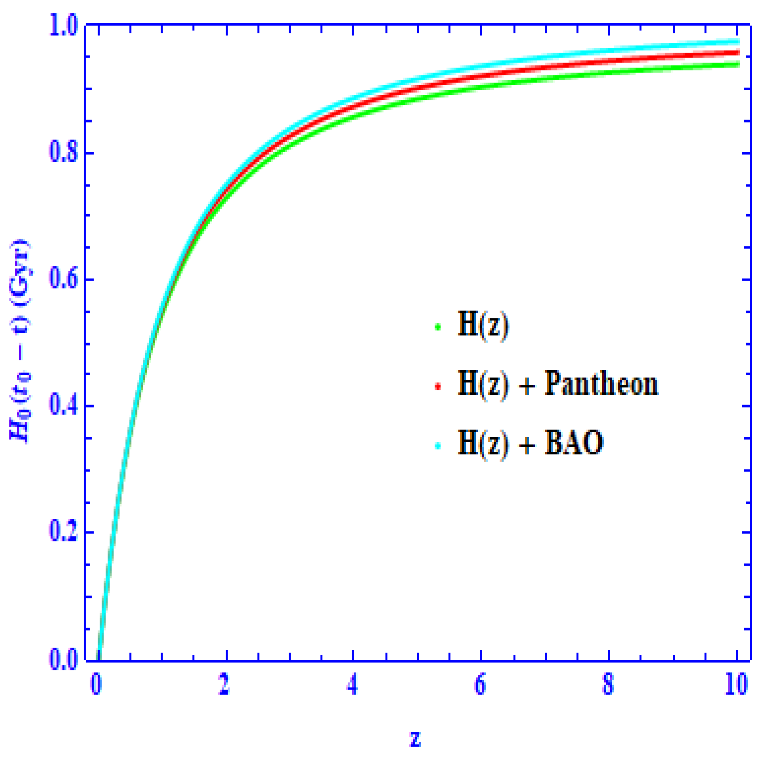
4.1. Age of Universe
The age of the Universe in the derived model is computed as
Therefore, the present age of the Universe is obtained as
where denotes the present age of the Universe.
Figure 7 depicts the variation of with respect to redshift z. Note that we considered the estimated values of , and in this paper by bounding the derived model with , + Pantheon and + BAO data sets. Integrating Equation (31) for the values of , and given in Table 2, we obtain the present age of the Universe in this paper for , + Pantheon compilation of SN Ia data and + BAO data sets as Gyrs, Gyrs and Gyrs, respectively. It is worth noting that the empirical age of the Universe extracted in a Plank collaboration result [19] is given as Gyrs. In some other cosmological studies, the present age of the Universe is computed as Gyrs [81], Gyrs [82], Gyrs [83] and Gyrs [84]. Thus, we observe that the age of the Universe estimated in the derived model is in good agreement with its value extracted in Plank collaboration [19]. It is important to note that the estimated age of the Universe due to joint and Pantheon compilation of SN Ia data in this paper, i.e., has only tension with the Plank collaboration result [19]. Some useful remarks on the age of the Universe and its curvature are given in Ref. [85].
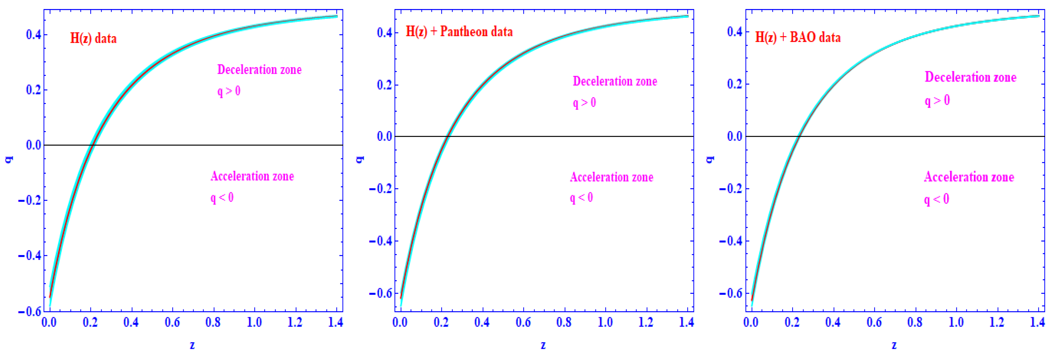
4.2. Deceleration Parameter
Equation (22) is recast as
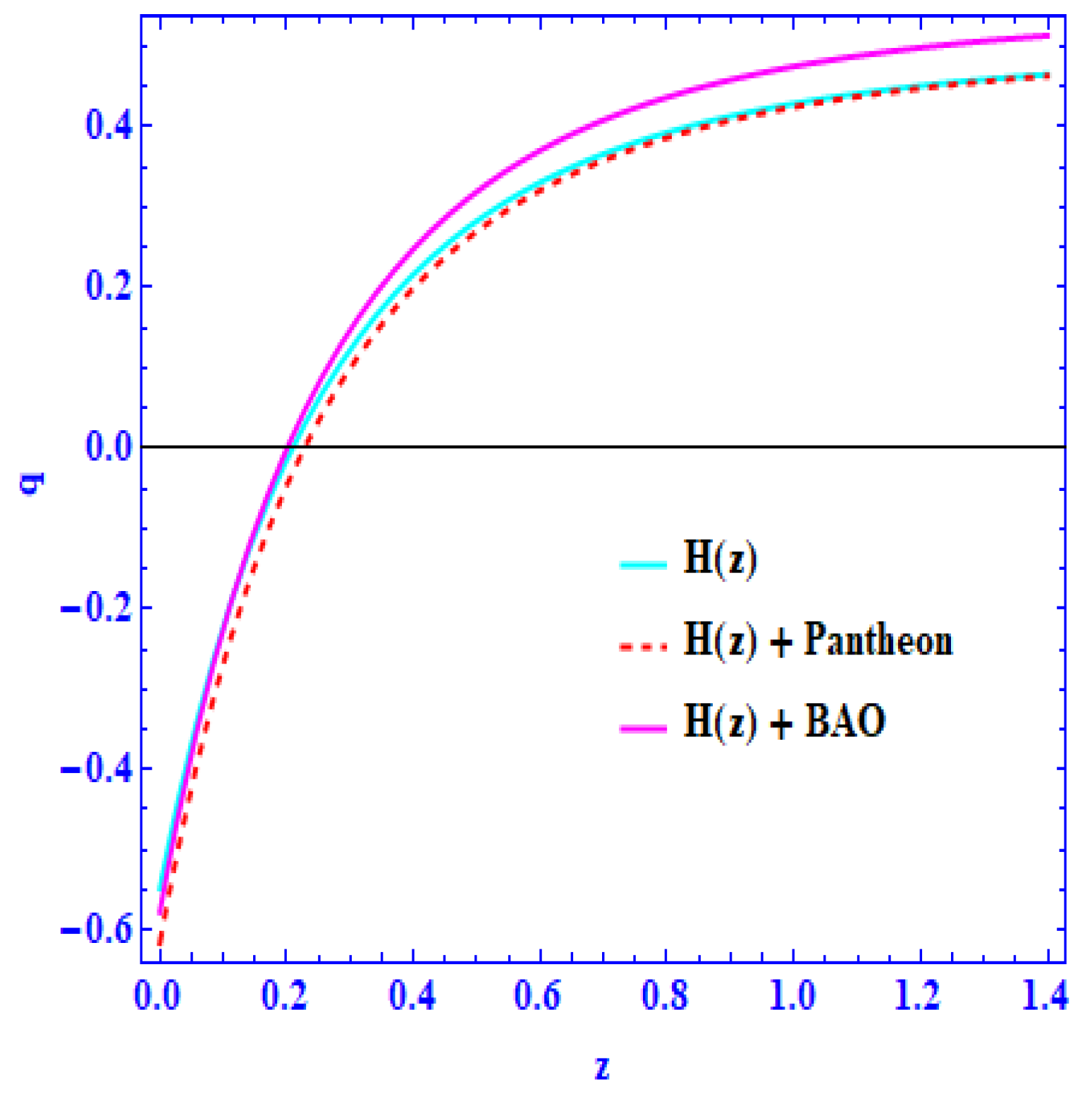
Figure 8 depicts the dynamics of deceleration parameter q with respect to redshift z for data (left panel, + Pantheon compilation of SN Ia data (middle panel) and + BAO data (right panel). We obtain the present value of deceleration parameter as , and by bounding the Universe in the derived model with , + Pantheon compilation of SN Ia and + BAO data sets, respectively. Figure 9 shows a single plot of q versus z. Recently, Capozziello et al. [86] obtained the empirical value of as . Some other empirical values of in the vicinity of our obtained values of are given in Refs. [87,88,89,90,91,92].
4.3. Statefinder Diagnostics
The statefinder pairs are the geometrical quantities which are directly obtained from the metric. This diagnostic is used to distinguish different dark energy models and hence becomes an important tool in modern cosmology. Alam et al. [93,94] defined the statefinder parameters r and s as follows
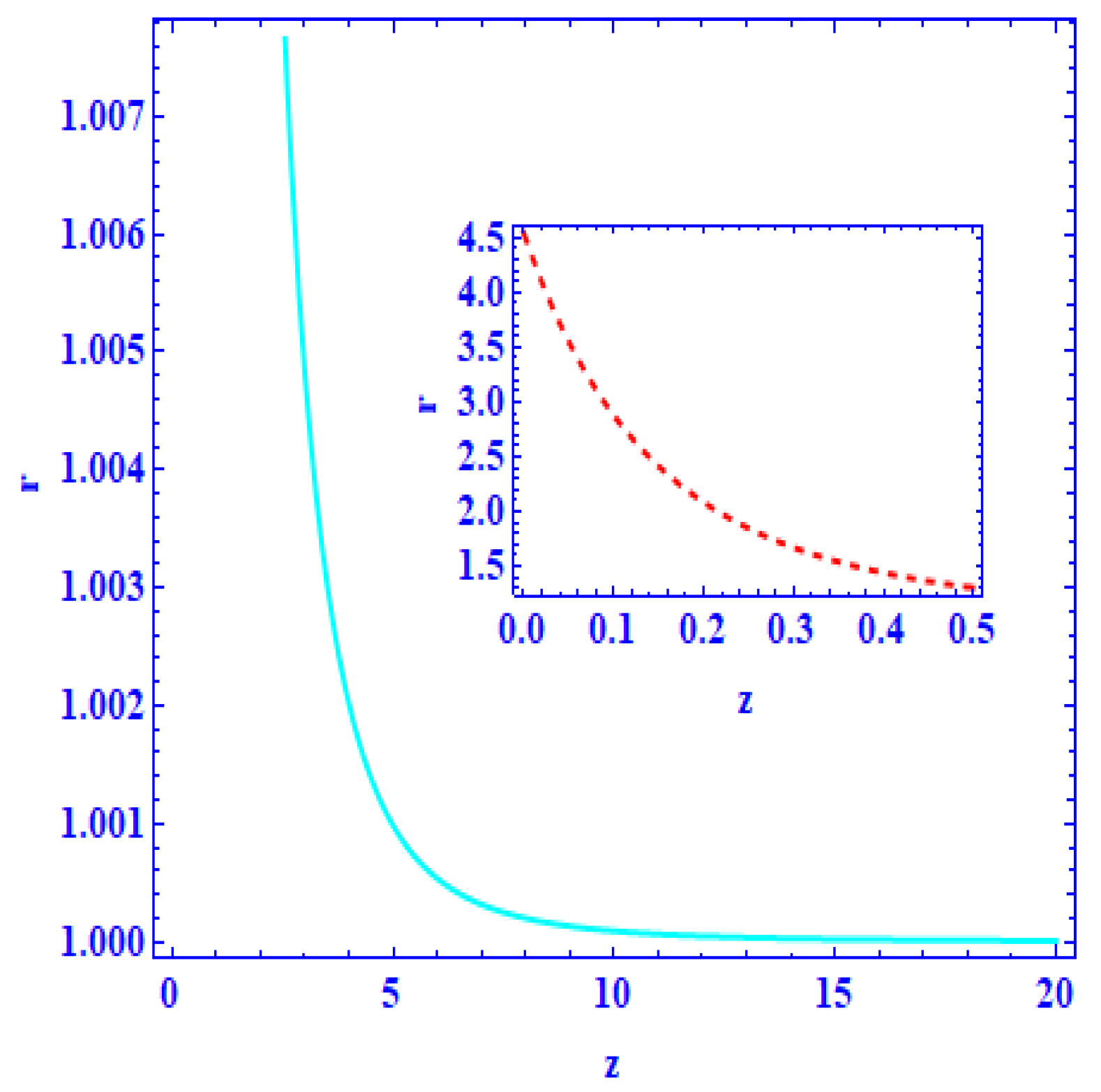
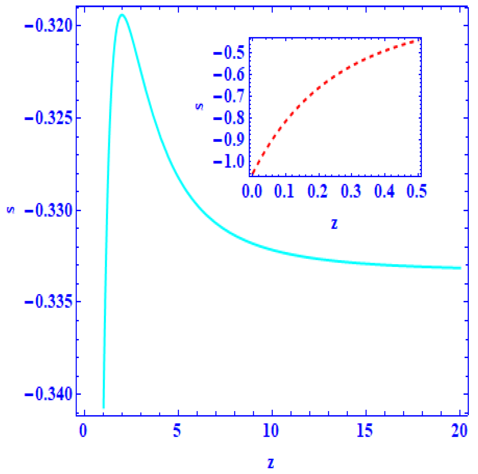
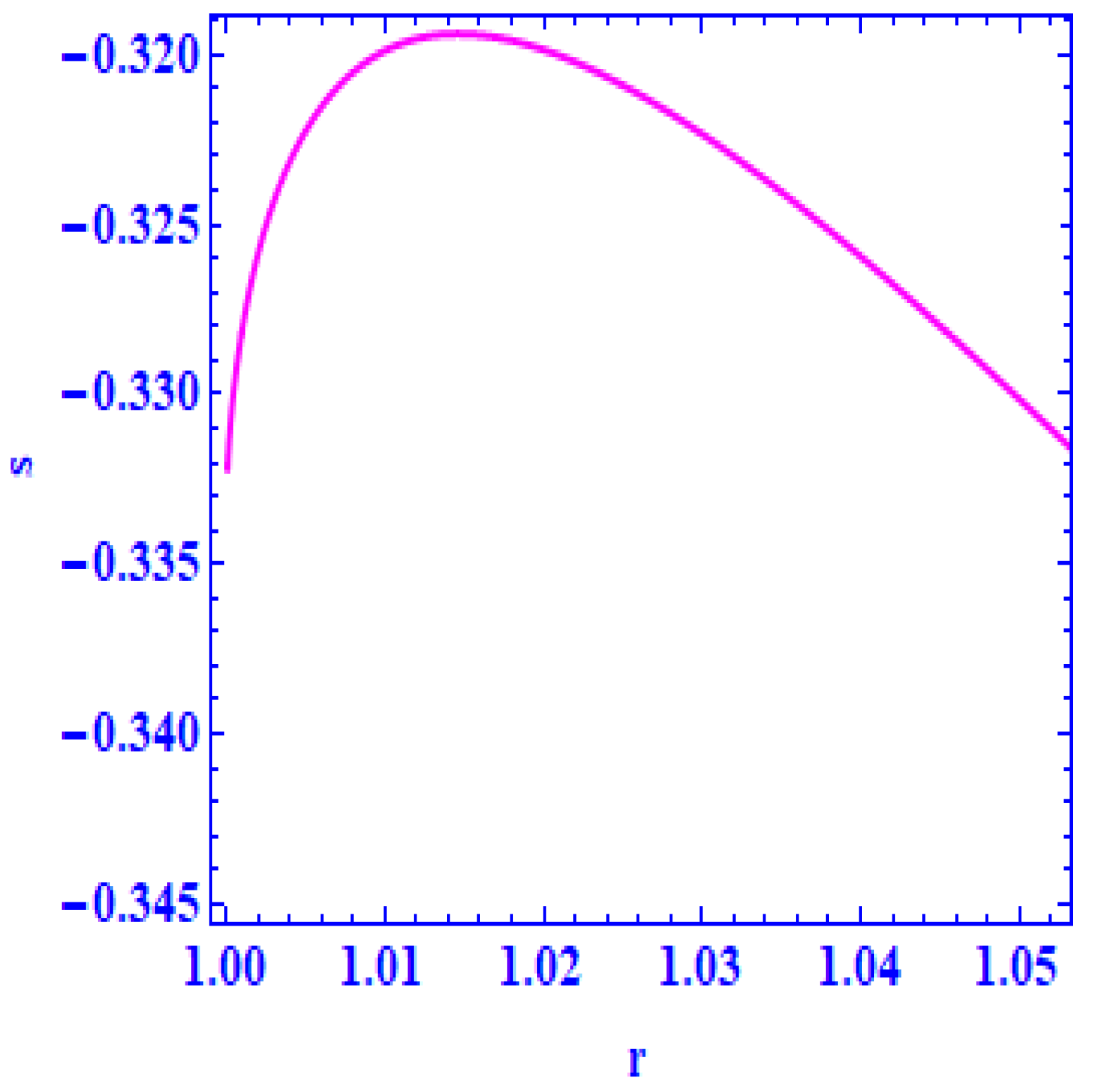
Figure 10 and Figure 11 exhibit the behaviour of r and s with respect to z, respectively. We compute and for joint and pantheon compilation of SN Ia data at . From Figure 10 and Figure 11, we observe that and in the redshift range . In addition, the Universe in the derived model presumes the values of statefinder pairs in the range and and therefore represents a Chaplygin gas-type dark energy model (CGDE). We draw the temporal evolution of the Universe mimicked by our model in Figure 12. The trajectory in the plane clearly shows that the profile starts from the region and which corresponds to the CGDE Universe.
The expression of r in terms of q and z is obtained as
5. Concluding Remarks
In this paper, we have investigated the late time accelerated expansion of the Universe by taking into account the scalar field with positive potential. To obtain an explicit solution of the field equations, we considered the simplest parametrization of the equation of state parameter . This parametrization gives at the present epoch. The scalar field potential is directly connected to pressure through equation ; therefore, the pressure is negative when , and hence, is responsible for negative pressure that leads the acceleration of the Universe in the derived model. We used data, Pantheon compilation of SN Ia data and BAO data to constrain the model parameters using a minimization technique. The constrained values of , and from all data sets are given in Table 2.
Furthermore, we also estimated the present age of the Universe as Gyrs, Gyrs and Gyrs by using , + Pantheon compilation of SN Ia data and + BAO data, respectively. Moreover, our estimated age of the Universe in the derived model due to combined and Pantheon compilation of SN Ia data has only tension compared to the Plank collaboration results [19]. In additon, the values of tensions that we obtain are 0.37 and 6.5 for combined and BAO data and combined H(z) and Pantheon compilation of SN Ia data, respectively, when we compare our results with the value of given in Plank collaboration [22]. Moreover, the tensions in this paper are 3.3 and 2.62 for combined and BAO data and combined H(z) and Pantheon compilation of SN Ia data, respectively, in comparing our value with R19 [23]. The Universe in the derived model evolves with a positive deceleration parameter in its early phase of expansion, and after dominance of the scalar field, the Universe evolves with a negative value of the deceleration parameter which shows a transition from an early decelerated expanding phase to the current accelerated expanding phase. It is interesting to note the value of obtained in our model is in good agreement with the recent results as reported in Ref. [86]. Furthermore, to investigate the parametrization from a geometrical point of view, we also diagnose the statefinder pairs . We observe that the Universe in the derived model describes a Chaplygin gas-type dark energy model (CGDE). Furthermore, we note that the authors of Refs. [95,96] use similar data sets for constraining the observational parameters of the Universe. In Bouali et al. [96], the present acceleration of the Universe is described by taking into consideration the parameterized deceleration parameter . As a final comment, we note from the above comparative study that the present model may be a viable model to describe the late time acceleration of the Universe and observational constraint update for the scalar field as dark energy.
Author Contributions
P.S.: Writing—original draft. A.J.K.: Review & editing. M.K.: Writing—original draft, Methodology, Writing—review & editing. G.G.: Writing—original draft, Writing—review & editing. J.K.S.: Review & editing. A.K.Y.: Writing—original draft, Conceptualization, Methodology, Writing—review & editing. All authors have read and agreed to the published version of the manuscript.
Funding
This research received no external funding.
Data Availability Statement
The data underlying this article will be shared on reasonable request to the authors.
Acknowledgments
The authors wish to place on record their sincere thanks to the reviewer(s) for illuminating suggestions that have significantly improved our manuscript in terms of research quality.
Conflicts of Interest
The authors declare no conflict of interest.
Appendix A

Table A1.
Hubble parameter H(z) with redshift and errors .
| S. N. | z | H(z) | Method | References | |
|---|---|---|---|---|---|
| 1 | 0 | 67.77 | 1.30 | DA | [97] |
| 2 | 0.07 | 69 | 19.6 | DA | [98] |
| 3 | 0.09 | 69 | 12 | DA | [99] |
| 4 | 0.01 | 69 | 12 | DA | [100] |
| 5 | 0.12 | 68.6 | 26.2 | DA | [98] |
| 6 | 0.17 | 83 | 8 | DA | [100] |
| 7 | 0.179 | 75 | 4 | DA | [101] |
| 8 | 0.1993 | 75 | 5 | DA | [101] |
| 9 | 0.2 | 72.9 | 29.6 | DA | [98] |
| 10 | 0.24 | 79.7 | 2.7 | DA | [102] |
| 11 | 0.27 | 77 | 14 | DA | [100] |
| 12 | 0.28 | 88.8 | 36.6 | DA | [98] |
| 13 | 0.35 | 82.7 | 8.4 | DA | [103] |
| 14 | 0.352 | 83 | 14 | DA | [101] |
| 15 | 0.38 | 81.5 | 1.9 | DA | [104] |
| 16 | 0.3802 | 83 | 13.5 | DA | [105] |
| 17 | 0.4 | 95 | 17 | DA | [99] |
| 18 | 0.4004 | 77 | 10.2 | DA | [105] |
| 19 | 0.4247 | 87.1 | 11.2 | DA | [105] |
| 20 | 0.43 | 86.5 | 3.7 | DA | [102] |
| 21 | 0.44 | 82.6 | 7.8 | DA | [106] |
| 22 | 0.44497 | 92.8 | 12.9 | DA | [105] |
| 23 | 0.47 | 89 | 49.6 | DA | [107] |
| 24 | 0.4783 | 80.9 | 9 | DA | [105] |
| 25 | 0.48 | 97 | 60 | DA | [100] |
| 26 | 0.51 | 90.4 | 1.9 | DA | [104] |
| 27 | 0.57 | 96.8 | 3.4 | DA | [108] |
| 28 | 0.593 | 104 | 13 | DA | [101] |
| 29 | 0.6 | 87.9 | 6.1 | DA | [106] |
| 30 | 0.61 | 97.3 | 2.1 | DA | [104] |
| 31 | 0.68 | 92 | 8 | DA | [101] |
| 32 | 0.73 | 97.3 | 7 | DA | [106] |
| 33 | 0.781 | 105 | 12 | DA | [101] |
| 34 | 0.875 | 125 | 17 | DA | [101] |
| 35 | 0.88 | 90 | 40 | DA | [100] |
| 36 | 0.9 | 117 | 23 | DA | [100] |
| 37 | 1.037 | 154 | 20 | DA | [101] |
| 38 | 1.3 | 168 | 17 | DA | [100] |
| 39 | 1.363 | 160 | 33.6 | DA | [109] |
| 40 | 1.43 | 177 | 18 | DA | [100] |
| 41 | 1.53 | 140 | 14 | DA | [100] |
| 42 | 1.75 | 202 | 40 | DA | [100] |
| 43 | 1.965 | 186.5 | 50.4 | DA | [109] |
| 44 | 2.3 | 224 | 8 | DA | [110] |
| 45 | 2.34 | 222 | 7 | DA | [111] |
| 46 | 2.36 | 226 | 8 | DA | [112] |
References
- Kumar, S.; Yadav, A.K. Some Bianchi type V models of accelerating universe with dark energy. Mod. Phys. Lett. A 2011, 26, 647. [Google Scholar] [CrossRef]
- Yadav, A.K. Some anisotropic dark energy models in Bianchi type-V space-time. Astrophys. Space Sc. 2011, 335, 565. [Google Scholar] [CrossRef]
- Yadav, A.K. A transitioning universe with anisotropic dark energy. Astrophys. Space Sc. 2016, 361, 1. [Google Scholar] [CrossRef]
- Goswami, G.K.; Yadav, A.K.; Mishra, B. Probing kinematics and fate of Bianchi type V Universe. Mod. Phys. Lett. A 2020, 35, 2050224. [Google Scholar] [CrossRef]
- Amirhashchi, H.; Yadav, A.K.; Ahmad, N.; Yadav, V. Interacting Dark Sectors in Anisotropic Universe: Observational Constraints and H0 Tension. Phys. Dark Uni. 2022, 36, 2022. [Google Scholar] [CrossRef]
- Goswami, G.K.; Mishra, M.; Yadav, A.K.; Pradhan, A. Two Fluid Scenario in Bianchi Type-I Universe. Mod. Phys. Lett. A 2020, 33, 2050086. [Google Scholar] [CrossRef]
- Kumar, S.; Singh, C.P. Anisotropic dark energy models with constant deceleration parameter. Gen. Relativ. Grav. 2011, 43, 1427. [Google Scholar] [CrossRef]
- Akarsu, Ö; Kılınc, C.B. Bianchi type III models with anisotropic dark energy. Gen. Relativ. Grav. 2010, 42, 763. [Google Scholar] [CrossRef]
- Harko, T.; Lobo, F.S.N.; Nojiri, S.; Odintsov, S.D. f (R, T) gravity. Phys. Rev. D 2011, 84, 024020. [Google Scholar] [CrossRef]
- Prasad, R.; Gupta, L.K.; Goswami, G.K.; Yadav, A.K. Bulk viscous accelerating Universe in f(R,T) theory of gravity. Pramana J. Physics 2020, 94, 135. [Google Scholar] [CrossRef]
- Yadav, A.K.; Sahoo, P.K.; Bhardwaj, V. Bulk Viscous Bianchi-I Embedded Cosmological Model in f (R, T)=f1(R)+f2(R)f3(T) Gravity. Mod. Phys. Lett. A 2019, 34, 1950145. [Google Scholar] [CrossRef]
- Sharma, L.K.; Yadav, A.K.; Sahoo, P.K.; Singh, B.K. Non-Minimal Matter-Geometry Coupling in Bianchi-I Space-Time. Results Phys. 2018, 10, 738. [Google Scholar] [CrossRef]
- Perlmutter, S.; Gabi, S.; Goldhaber, G.; Goobar, A.; Groom, D.E.; Hook, I.M.; Kim, A.G.; Kim, M.Y.; Lee, J.C.; Pain, R.; et al. Measurements of the Cosmological Parameters Ω and Λ from the First Seven Supernovae at z ≥ 0.35. ApJ 1997, 483, 565. [Google Scholar] [CrossRef]
- Perlmutter, S.; Aldering, G.; Della Valle, M.; Deustua, S.; Ellis, R.S.; Fabbro, S.; Fruchter, A.; Goldhaber, G.; Groom, D.E.; Hook, I.M.; et al. Discovery of a supernova explosion at half the age of the Universe. Nature 1998, 391, 51. [Google Scholar] [CrossRef]
- Perlmutter, S.; Aldering, G.; Goldhaber, G.; Knop, R.A.; Nugent, P.; Castro, P.G.; Deustua, S.; Fabbro, S.; Goobar, A.; Groom, D.E.; et al. Measurements of Ω and Λ from 42 High-Redshift Supernovae. ApJ 1999, 517, 565. [Google Scholar] [CrossRef]
- Riess, A.G.; Strolger, L.-G.; Tonry, J.; Casertano, S.; Ferguson, H.C.; Mobasher, B.; Challis, P.; Filippenko, A.V.; Jha, S.; Li, W.; et al. Type Ia supernova discoveries at z > 1 from the Hubble space telescope: Evidence for past deceleration and constraints on dark energy evolution. ApJ 2004, 607, 665. [Google Scholar] [CrossRef]
- Blake, C.; Kazin, E.; Beutler, F.; Davis, T.; Parkinson, D.; Brough, S.; Colless, M.; Contreras, C.; Couch, W.; Croom, S.; et al. The WiggleZ Dark Energy Survey: Mapping the distance-redshift relation with baryon acoustic oscillations. MNRAS 2011, 418, 1707. [Google Scholar] [CrossRef]
- Bennett, C.; Hill, R.S.; Hinshaw, G.; Nolta, M.R.; Odegard, N.; Page, L.; Spergel, D.N.; Weiland, J.L.; Wright, E.L.; Halpern, M.; et al. First-Year Wilkinson Microwave Anisotropy Probe (WMAP) Observations: Foreground Emission. ApJS 2003, 148, 1. [Google Scholar] [CrossRef]
- Ade, P.A.R.; Aghanim, N.; Arnaud, M.; Ashdown, M.; Aumont, J.; Baccigalupi, C.; Banday, A.J.; Barreiro, R.B.; Bartlett, J.G.; Bartolo, N.; et al. [Planck Collaboration.] Planck 2015 results XIII Cosmological parameters. Astron. Astrophys. 2016, 594, A13. [Google Scholar]
- Weinberg, S. The cosmological constant problem. Rev. Mod. Phys. 1989, 61, 1. [Google Scholar] [CrossRef]
- Peebles, P.; Ratra, B. The cosmological constant and dark energy. Rev. Mod. Phys. 2003, 75, 559. [Google Scholar] [CrossRef]
- Aghanim, N.; Akrami, Y.; Ashdown, M.; Aumont, J.; Baccigalupi, C.; Ballardini, M.; Banday, A.J.; Barreiro, R.B.; Bartolo, N.; Basak, S.; et al. Planck 2018 results. VI. Cosmological parameters. arXiv 2018, arXiv:1807.06209. [Google Scholar]
- Riess, A.G.; Casertano, S.; Yuan, W.; Macri, L.M.; Scolnic, D. Large magellanic cloud cepheid standards provide a 1% foundation for the determination of the Hubble Constant and stronger evidence for Physics beyond ΛCDM. Astrophys. J. 2019, 876, 85. [Google Scholar] [CrossRef]
- Riess, A.G.; Casertano, S.; Yuan, W.; Bowers, J.B.; Macri, L.; Zinn, J.C.; Scolnic, D. Cosmic Distances Calibrated to 1% Precision with Gaia EDR3 Parallaxes and Hubble Space Telescope Photometry of 75 Milky Way Cepheids Confirm Tension with LambdaCDM. arXiv 2020, arXiv:2012.08534. [Google Scholar] [CrossRef]
- Valentino, E.D.; Pan, S.; Yang, W.; Anchordoqui, L.A. Touch of neutrinos on the vacuum metamorphosis: Is the H0 Solution Back? Phys. Rev. D 2021, 103, 123527. [Google Scholar] [CrossRef]
- Banerjee, A.; Cai, H.; Heisenberg, L.; Colgain, E.O.; Sheikh-Jabbari, M.M.; Yang, T. Hubble Sinks In The Low-Redshift Swampland. Phys. Rev. D 2021, 103, 081305. [Google Scholar] [CrossRef]
- Capozziello, S.; Carloni, S.; Troisi, A. Quintessence without scalar fields. Recent Res. Dev. Astron. Asrophys. 2003, 1, 625. [Google Scholar]
- Harko, T. Thermodynamic interpretation of the generalized gravity models with geometry-matter coupling. Phys. Rev. D 2014, 90, 044067. [Google Scholar] [CrossRef]
- Bhardwaj, V.K.; Yadav, A.K. Some Bianchi type V accelerating cosmological models in f (R, T) = f1(R) + f2(T) formalism. Int. J. Geom. Meth. Mod. Phys. 2020, 7, 2050159. [Google Scholar] [CrossRef]
- Yadav, A.K.; Mondal, M.; Rahaman, F. Singularity-free nonexotic compact star in f(R,T) gravity. Pramana J. Phys. 2020, 94, 90. [Google Scholar] [CrossRef]
- Sharma, L.K.; Yadav, A.K.; Singh, B.K. Power-law solution for homogeneous and isotropic universe in f(R, T) gravity. New Astron. 2020, 79, 101396. [Google Scholar] [CrossRef]
- Singla, N.; Gupta, M.K.; Yadav, A.K. Accelerating model of flat universe in f (R, T) gravity. Grav. Cosmol. 2020, 26, 144. [Google Scholar] [CrossRef]
- Yadav, A.K.; Ali, A.T. Invariant Bianchi type I models in f(R,T) Gravity. Int. J. Geom. Methods. Mod. Phys. 2018, 15, 1850026. [Google Scholar] [CrossRef]
- Yadav, A.K.; Srivastava, P.K.; Yadav, L. Hybrid expansion law for dark energy dominated universe in f(R,T) Gravity. Int. J. Theor. Phys. 2015, 54, 1671. [Google Scholar] [CrossRef]
- Hu, W.; Sawicki, I. Models of f (R) cosmic acceleration that evade solar system tests. Phys. Rev. D 2007, 76, 064004. [Google Scholar] [CrossRef]
- Nojiri, S.; Odintsov, S.D. Modified gravity with negative and positive powers of curvature: Unification of inflation and cosmic acceleration. Phys. Rev. D 2003, 68, 123512. [Google Scholar] [CrossRef]
- Capozziello, S.; Cardone, V.F.; Troisi, A. Dark energy and dark matter as curvature effects. JCAP 2006, 0608, 001. [Google Scholar]
- Martins, C.F.; Salucci, P. Analysis of Rotation Curves in the framework of Rn gravity. Mon. Not. R. Astron. Soc. 2007, 381, 1103. [Google Scholar] [CrossRef]
- Boehmer, C.G.; Harko, T.; Lobo, F.S.N. Dark matter as a geometric effect in f (R) gravity. Astropart. Phys. 2008, 29, 386. [Google Scholar] [CrossRef]
- Boehmer, C.G.; Harko, T.; Lobo, F.S.N. Generalized virial theorem in f(R) gravity. JCAP 2008, 03, 024. [Google Scholar] [CrossRef]
- De Felice, A.; Tsujikawa, S. Construction of cosmologically viable f (G) gravity models. Phys. Lett. B 2009, 675, 1. [Google Scholar] [CrossRef]
- Bamba, K.; Odintsov, S.D.; Sebastiani, L.; Zerbini, S. Finite-time future singularities in modified Gauss-Bonnet and F(R, G) gravity and singularity avoidance. Eur. Phys. J. C 2010, 67, 295. [Google Scholar] [CrossRef]
- Bahamonde, S.; Zubair, M.; Abbas, G. Thermodynamics and cosmological reconstruction in f (T, B gravity. Phys. Dark Univ. 2018, 19, 78. [Google Scholar] [CrossRef]
- Nojiri, S.; Odintsov, S.D.; Oikonomou, V.K. Modified gravity theories on a nutshell: Inflation, bounce and late-time evolution. Phys. Rept. 2017, 692, 1. [Google Scholar] [CrossRef]
- Oikonomou, V.K. Rescaled Einstein-Hilbert gravity from F(R) gravity: Inflation, dark energy, and the swampland criteria. Phys. Rev. D 2021, 103, 124028. [Google Scholar] [CrossRef]
- Oikonomou, V.K. Unifying inflation with early and late dark energy epochs in axion F(R) gravity. Phys. Rev. D 2021, 103, 044036. [Google Scholar] [CrossRef]
- Odintsov, S.D.; Oikonomou, V.K. Geometric inflation and dark energy with axion F(R) gravity. Phys. Rev. D 2020, 101, 044009. [Google Scholar] [CrossRef]
- Odintsov, S.D.; Oikonomou, V.K. Unification of inflation with dark energy in F(R) gravity and axion dark matter. Phys. Rev. D 2019, 99, 104070. [Google Scholar] [CrossRef]
- Yousaf, Z. Stellar filaments with Minkowskian core in the Einstein - Λ gravity. Eur. Phys. J. Plus 2017, 132, 71. [Google Scholar] [CrossRef]
- Yousaf, Z. On the role of f (G, T) terms in structure scalars. Eur. Phys. J. Plus 2019, 134, 245. [Google Scholar] [CrossRef]
- Yousaf, Z.; Bamba, K.; Bhatti, M.Z. Causes of irregular energy density in f(R,T) gravity. Phys. Rev. D 2016, 93, 124048. [Google Scholar] [CrossRef]
- Caldwell, R.R.; Dave, R.; Steinhardt, P.J. Cosmological Imprint of an Energy Component with General Equation of State. Phys. Rev. Lett 1998, 80, 1582. [Google Scholar] [CrossRef]
- Ferreira, P.G.; Joyce, M. Cosmology with a primordial scaling field. Phys. Rev. D 1998, 58, 023503. [Google Scholar] [CrossRef]
- Copel, E.J.; Liddle, A.R.; Wands, D. Exponential potentials and cosmological scaling solutions. Phys. Rev. D 1998, 57, 4686. [Google Scholar]
- Liddle, A.R.; Scherrer, R.J. Classification of scalar field potentials with cosmological scaling solutions. Phys. Rev. D 1998, 59, 023509. [Google Scholar] [CrossRef]
- Dodleson, S.; Kaplinghat, M.; Stewart, E. Solving the Coincidence Problem: Tracking Oscillating Energy. Phys. Rev. Lett. 2000, 85, 5276. [Google Scholar] [CrossRef]
- Zlatev, I.; Wang, L.; Steinhardt, P.J. Quintessence, Cosmic Coincidence, and the Cosmological Constant. Phys. Rev. Lett. 1999, 82, 896. [Google Scholar] [CrossRef]
- Steinhardt, P.J.; Wang, L.; Zlatev, I. Cosmological tracking solutions. Phys. Rev. D 1999, 59, 123504. [Google Scholar] [CrossRef]
- Johri, V.B. Search for tracker potentials in quintessence theory. Class. Quant. Grav. 2002, 19, 5959. [Google Scholar] [CrossRef]
- Johri, V.B. Genesis of cosmological tracker fields. Phys. Rev. D 2001, 63, 103504. [Google Scholar] [CrossRef]
- Sahni, V. Dark matter and dark energy. Lect. Notes Phys. 2004, 653, 141. [Google Scholar]
- Sahni, V.; Starobinsky, A. The Case for a Positive Cosmological Lambda-term. Int. J. Mod. Phys. D 2000, 9, 373. [Google Scholar] [CrossRef]
- Chimento, L.P.; Jakubi, A.S. Scalar field cosmologies with perfect fluid in Robertson-Walker metric. Int. J. Mod. Phys. D 1996, 5, 71. [Google Scholar] [CrossRef]
- Hartle, J.B.; Hawking, S.W. Wave function of the Universe. Phys. Rev. D 1983, 28, 2960. [Google Scholar] [CrossRef]
- Hawking, S.W. The quantum state of the universe. Nucl. Phys. B 1984, 239, 257. [Google Scholar] [CrossRef]
- Vilenkin, A. Creation of universes from nothing. Phys. Lett. B 1982, 117, 25. [Google Scholar] [CrossRef]
- Barvinsky, A.O. Unitarity approach to quantum cosmology. Phys. Rep. 1993, 230, 237. [Google Scholar] [CrossRef]
- Spokoiny, B.L. Inflation and generation of perturbations in broken-symmetric theory of gravity. Phys. Lett. B 1984, 147, 39. [Google Scholar] [CrossRef]
- Salopek, D.S.; Bond, J.R.; Bardeen, J.M. Designing density fluctuation spectra in inflation. Phys. Rev. D 1989, 40, 1753. [Google Scholar] [CrossRef]
- Khalatnikov, I.M.; Mezhlumian, A. The classical and quantum cosmology with a complex scalar field. Phys. Lett. A 1992, 169, 308. [Google Scholar] [CrossRef]
- Kamenshchik, A.Y.; Moschella, U.; Pasquier, V. An alternative to quintessence. Phys. Lett. B 2001, 511, 265. [Google Scholar] [CrossRef]
- Gong, Y.; Zhang, Y. Probing the curvature and dark energy. Phys. Rev. D 2005, 72, 043518. [Google Scholar] [CrossRef]
- Sharov, G.S.; Vasiliev, V.O. How predictions of cosmological models depend on Hubble parameter data sets. Math. Model. Geom. 2018, 6, 1. [Google Scholar] [CrossRef]
- Biswas, P.; Roy, P.; Biswas, R. Posing constraints on the free parameters of a new model of dark energy EoS: Responses through cosmological behaviours. arXiv 2019, arXiv:1908.00408. [Google Scholar] [CrossRef]
- Scolnic, D.M.; Jones, D.O.; Rest, A.; Pan, Y.C.; Chornock, R.; Foley, R.J.; Huber, M.E.; Kessler, R.; Narayan, G.; Riess, A.G.; et al. The Complete Light-curve Sample of Spectroscopically Confirmed SNe Ia from Pan-STARRS1 and Cosmological Constraints from the Combined Pantheon Sample. Astrophys. J. 2018, 859, 101. [Google Scholar] [CrossRef]
- Beutler, F.; Blake, C.; Colless, M.; Heath Jones, D.; Staveley-Smith, L.; Campbell, L.; Parker, Q.; Saunders, W.; Watson, F. The 6dF Galaxy Survey: Baryon acoustic oscillations and the local Hubble constant. MNRAS 2011, 416, 3017. [Google Scholar] [CrossRef]
- Padmanabhan, N.; Xu, X.; Eisenstein, D.J.; Scalzo, R.; Cuesta, A.J.; Mehta, K.T.; Kazin, E. A 2 percent distance to z=0.35 by reconstructing baryon acoustic oscillations - I. Methods and application to the Sloan Digital Sky Survey. MNRAS 2012, 427, 2132. [Google Scholar] [CrossRef]
- Anderson, L.; Aubourg, E.; Bailey, S.; Bizyaev, D.; Blanton, M.; Bolton, A.S.; Brinkmann, J.; Brownstein, J.R.; Burden, A.; Cuesta, A.J.; et al. The clustering of galaxies in the SDSS-III Baryon Oscillation Spectroscopic Survey: Baryon acoustic oscillations in the Data Release 9 spectroscopic galaxy sample. MNRAS 2013, 427, 3435. [Google Scholar] [CrossRef]
- Blake, C.; Brough, S.; Colless, M.; Contreras, C.; Couch, W.; Croom, S.; Davis, T.; Drinkwater, M.J.; Forster, K.; Gilbank, D.; et al. The WiggleZ Dark Energy Survey: The growth rate of cosmic structure since redshift z=0.9. MNRAS 2011, 415, 2876. [Google Scholar] [CrossRef]
- Hinshaw, G.; Larson, D.; Komatsu, E.; Spergel, D.N.; Bennett, C.L.; Dunkley, J.; Nolta, M.R.; Halpern, M.; Hill, R.S.; Odegard, N.; et al. Nine-year Wilkinson Microwave Anisotropy Probe (WMAP) Observations: Cosmological Parameter Results. Astrophys. J. Suppl. Ser. 2013, 208, 19. [Google Scholar] [CrossRef]
- Bond, H.E.; Nelan, E.P.; VandenBerg, D.A.; Schaefer, G.H.; Harmer, D. HD 140283: A star in the solar neighborhood that formed shortly after big bang. Astrophys. J. 2013, 765, L12. [Google Scholar] [CrossRef]
- Masi, S.; Ade, P.A.R.; Bock, J.J.; Bond, J.R.; Borrill, J.; Boscaleri, A.; Coble, K.; Contaldi, C.R.; Crill, B.P.; De Bernardis, P.; et al. The BOOMERanG experiment and the curvature of the universe. Prog. Part. Nucl. Phys. 2002, 48, 243. [Google Scholar] [CrossRef]
- Yadav, A.K.; Alshehri, A.M.; Ahmad, N.; Goswami, G.K.; Kumar, M. Transitioning universe with hybrid scalar field in Bianchi I space-time. Phys. Dark Uni. 2021, 31, 100738. [Google Scholar] [CrossRef]
- Renzini, A.; Bragaglia, A.; Ferraro, F.R. The white dwarf distance to the globular cluster NGC 6752 (and its age) with the HUBBLE SPACE TELESCOPE. Astrophys. J. 1996, 465, L23. [Google Scholar] [CrossRef]
- Valentino, E.D.; Anchordoqu, L.A.; Akarsu, Ö.; Ali-Haimoud, Y.; Amendola, L.; Arendse, N.; Asgar, M.; Ballardini, M.; Basilakos, S.; Battistelli, E.; et al. Cosmology Intertwined IV The Age of the Universe and its Curvature. Astropart. Phys. 2021, 131, 102607. [Google Scholar] [CrossRef]
- Capozziello, S.; Agostino, R.D.; Luongo, O. High-redshift cosmography: Auxiliary variables versus Pade polynomials. Mon. Not. Roy. Astron. Soc. 2020, 494, 2576. [Google Scholar] [CrossRef]
- Cunha, C.E.; Lima, M.; Oyaizu, H.; Frieman, J.; Lin, H. Estimating the redshift distribution of photometric galaxy samples – II. Applications and tests of a new method. Mon. Not. Roy. Astron. Soc. 2009, 396, 2379. [Google Scholar] [CrossRef]
- Jesus, J.F.; Valentim, R.; Escobal, A.A.; Pereira, S.H. Gaussian process estimation of transition redshift. J. Cosm. Astrop. Phys. 2020, 04, 053. [Google Scholar] [CrossRef]
- Singla, N.; Gupta, M.K.; Yadav, A.K.; Goswami, G.K. Accelerating universe with binary mixture of bulk viscous fluid and dark energy. Int. J. Mod. Phys. A 2021, 36, 2150148. [Google Scholar] [CrossRef]
- Prasad, R.; Gupta, L.K.; Yadav, A.K. Lyra’s cosmology of homogeneous and isotropic universe in Brans-Dicke theory. Int. J. Geom. Meth. Mod. Phys. 2021, 18, 2150029. [Google Scholar] [CrossRef]
- Prasad, R.; Gupta, L.K.; Beeshan, A.; Goswami, G.K.; Yadav, A.K. Bianchi type I universe: An extension of ΛCDM model. Int. J. Geom. Meth. Mod. Phys. 2021, 18, 2150069. [Google Scholar] [CrossRef]
- Prasad, R.; Yadav, A.K.; Yadav, A.K. Constraining Bianchi type V universe with recent H(z) and BAO observations in Brans–Dicke theory of gravitation. Eur. Phys. J. Plus 2020, 135, 297. [Google Scholar] [CrossRef]
- Sahni, V.; Saini, T.D.; Starobinsky, A.A.; Alam, U. Statefinder - a new geometrical diagnostic of dark energy. JETP Lett. 2003, 77, 201. [Google Scholar] [CrossRef]
- Alam, U.; Sahni, V.; Saini, T.D.; Starobinsky, A.A. Exploring the Expanding Universe and Dark Energy using the Statefinder Diagnostic. Mon. Not. R. Astron. Soc. 2003, 344, 1057. [Google Scholar] [CrossRef]
- Tsagas, C.G. The deceleration parameter in ‘tilted’ universes: Generalising the Friedmann background. Euro. Phys. J. C 2022, 82, 521. [Google Scholar] [CrossRef]
- Bouali, A.; Chaudhary, H.; Debnath, U.; Roy, T.; Mustafa, G. Constraints on the Parameterized Deceleration Parameter in FRW Universe. arXiv 2023, arXiv:2301.12107. [Google Scholar]
- Macaulay, E.; Nichol, R.C.; Bacon, D.; Brout, D.; Davis, T.M.; Zhang, B.; Bassett, B.A.; Scolnic, D.; Moller, A.; D’Andrea, C.B.; et al. First cosmological results using Type Ia supernovae from the Dark Energy Survey: Measurement of the Hubble constant. arXiv 2018, arXiv:1811.02376. [Google Scholar] [CrossRef]
- Zhang, C.; Zhang, H.; Yuan, S.; Liu, S.; Zhang, T.J.; Sun, Y.C. Four New Observational H(z) Data From Luminous Red Galaxies of Sloan Digital Sky Survey Data Release Seven. Res. Astron. Astrophys. 2014, 14, 1221. [Google Scholar] [CrossRef]
- Simon, J.; Verde, L.; Jimenez, R. Constraints on the redshift dependence of the dark energy potential. Phys. Rev. D 2005, 71, 123001. [Google Scholar] [CrossRef]
- Stern, D.; Jimenez, R.; Verde, L.; Kamionkowski, M.; Stanford, S.A. Cosmic chronometers: Constraining the equation of state of dark energy I: H(z) measurements. JCAP 2010, 1002, 008. [Google Scholar] [CrossRef]
- Moresco, M.; Cimatti, A.; Jimenez, R.; Pozzetti, L.; Zamorani, G.; Bolzonella, M.; Dunlop, J.; Lamareille, F.; Mignoli, M.; Pearce, H. et al. Improved constraints on the expansion rate of the Universe up to z∼1.1 from the spectroscopic evolution of cosmic chronometers. JCAP 2012, 8, 006. [Google Scholar] [CrossRef]
- Gaztanaga, E.; Cabre, A.; Hui, L. Clustering of Luminous Red Galaxies IV: Baryon Acoustic Peak in the Line-of-Sight Direction and a Direct Measurement of H(z). MNRAS 2009, 399, 1663. [Google Scholar] [CrossRef]
- Chuang, D.H.; Wang, Y. Modelling the anisotropic two-point galaxy correlation function on small scales and single-probe measurements of H(z), DA(z) and f (z)σ8(z) from the Sloan Digital Sky Survey DR7 luminous red galaxies. MNRAS 2013, 435, 255. [Google Scholar] [CrossRef]
- Alam, S.; Ata, M.; Bailey, S.; Beutler, F.; Bizyaev, D.; Blazek, J.A.; Bolton, A.S.; Brownstein, J.R.; Burden, A.; Chuang, C.-H.; et al. The clustering of galaxies in the completed SDSS-III Baryon Oscillation Spectroscopic Survey: Cosmological analysis of the DR12 galaxy sample. MNRAS 2016, 470, 2617. [Google Scholar] [CrossRef]
- Moresco, M.; Pozzetti, L.; Cimatti, A.; Jimenez, R.; Maraston, C.; Verde, L.; Thomas, D.; Citro, A.; Tojeiro, R.; Wilkinson, D. A 6% measurement of the Hubble parameter at z∼0.45: Direct evidence of the epoch of cosmic re-acceleration. JCAP 2016, 5, 014. [Google Scholar] [CrossRef]
- Blake, C.; Brough, S.; Colless, M.; Contreras, C.; Couch, W.; Croom, S.; Croton, D.; Davis, T.M.; Drinkwater, M.J.; Forster, K.; et al. The WiggleZ Dark Energy Survey: Joint measurements of the expansion and growth history at z <1. MNRAS 2012, 425, 405. [Google Scholar]
- Ratsimbazafy, A.L.; Loubser, S.I.; Crawford, S.M.; Cress, C.M.; Bassett, B.A.; Nichol, R.C.; Vaisanen, P. Age-dating luminous red galaxies observed with the Southern African Large Telescope. MNRAS 2017, 467, 3239. [Google Scholar] [CrossRef]
- Anderson, L.; Aubourg, É.; Bailey, S.; Beutler, F.; Bhardwaj, V.; Blanton, M.; Bolton, A.S.; Brinkmann, J.; Brownstein, J.R.; Burden, A.; et al. The clustering of galaxies in the SDSS-III Baryon Oscillation Spectroscopic Survey: Baryon acoustic oscillations in the Data Releases 10 and 11 Galaxy samples. MNRAS 2014, 441, 24. [Google Scholar] [CrossRef]
- Moresco, M. Raising the bar: New constraints on the Hubble parameter with cosmic chronometers at z∼2. MNRAS 2015, 450, L16. [Google Scholar] [CrossRef]
- Busca, N.G.; Delubac, T.; Rich, J.; Bailey, S.; Font-Ribera, A.; Kirkby, D.; Le Goff, J.-M.; Pieri, M.M.; Slosar, A.; Aubourg, É.; et al. Baryon acoustic oscillations in the Lyα forest of BOSS quasars. Astron. Astrophys. 2013, 552, A96. [Google Scholar] [CrossRef]
- Rich, J. Which fundamental constants for cosmic microwave background and baryon-acoustic oscillation? Astron. Astrophys. 2015, 584, A69. [Google Scholar] [CrossRef]
- Font-Ribera, A.; Kirkby, D.; Busca, N.; Miralda-Escude, J.; Ross, N.P.; Slosar, A.; Rich, J.; Aubourg, E.; Bailey, S.; Bhardwaj, V.; et al. Quasar-Lyman α forest cross-correlation from BOSS DR11: Baryon Acoustic Oscillations. JCAP 2014, 1405, 027. [Google Scholar] [CrossRef]
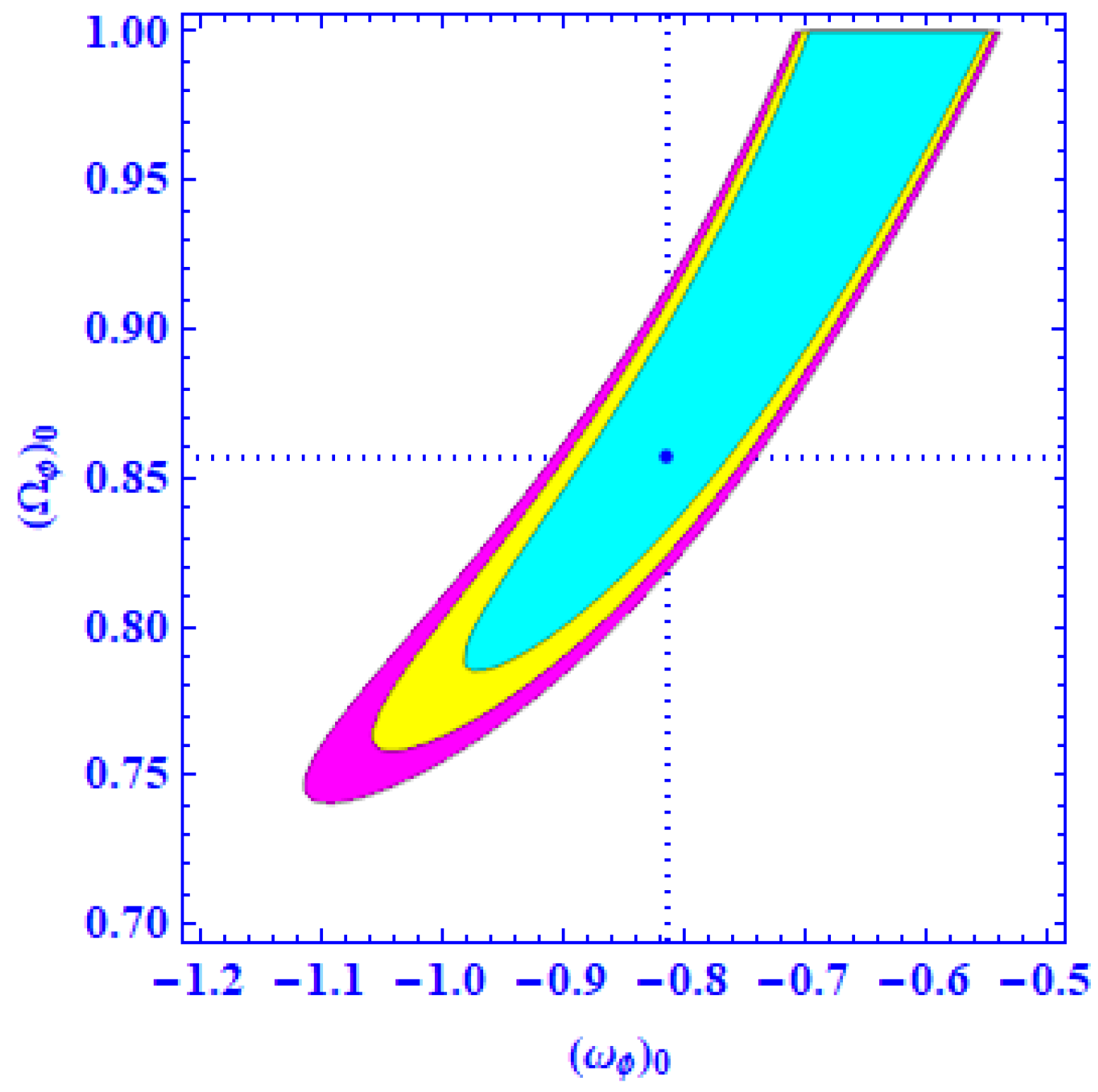
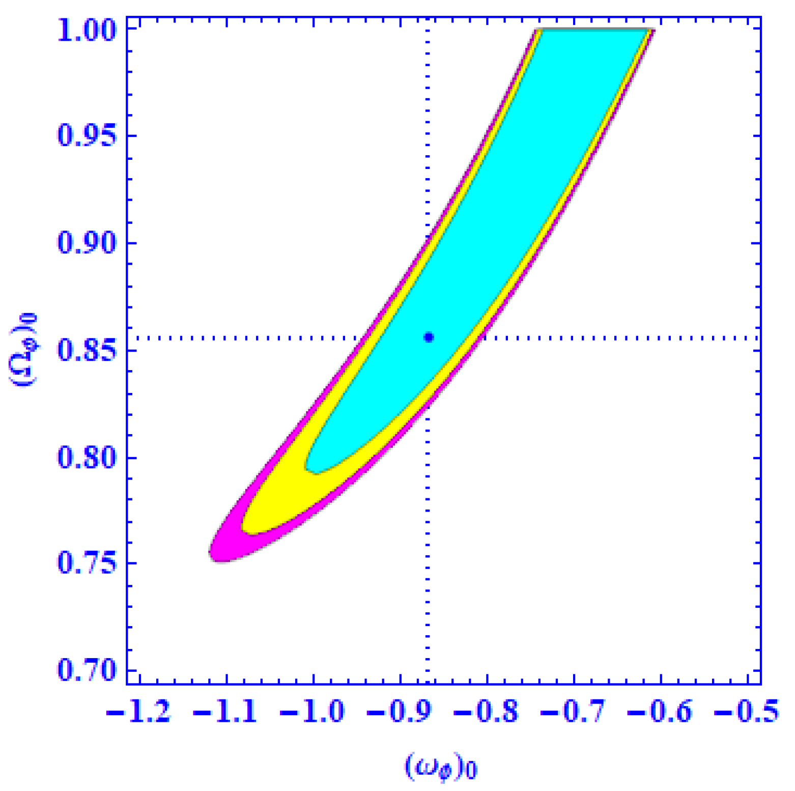
Figure 1.
Two-dimensional contours in the plane at , and confidence regions by bounding our model with data.
Figure 1.
Two-dimensional contours in the plane at , and confidence regions by bounding our model with data.

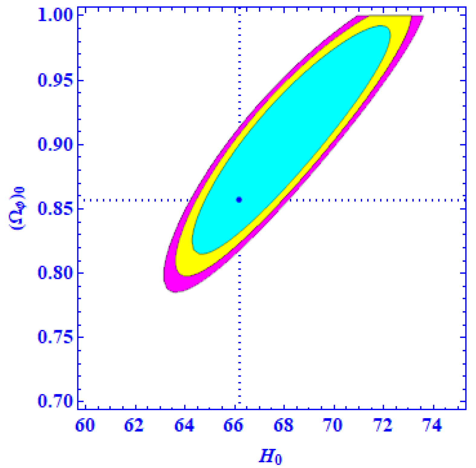
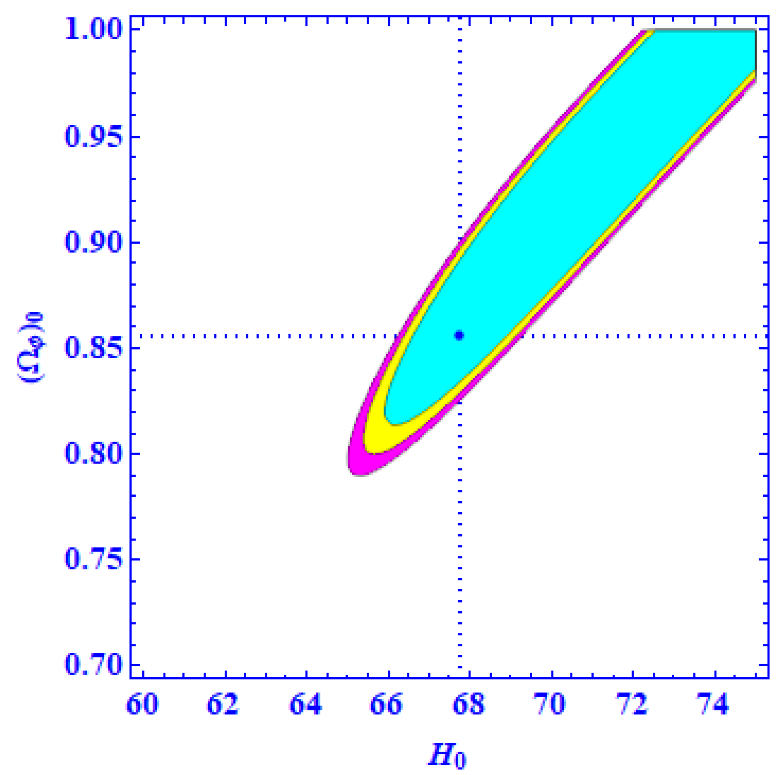
Figure 2.
Two-dimensional contours in the plane at , and confidence regions by bounding our model with data.
Figure 2.
Two-dimensional contours in the plane at , and confidence regions by bounding our model with data.

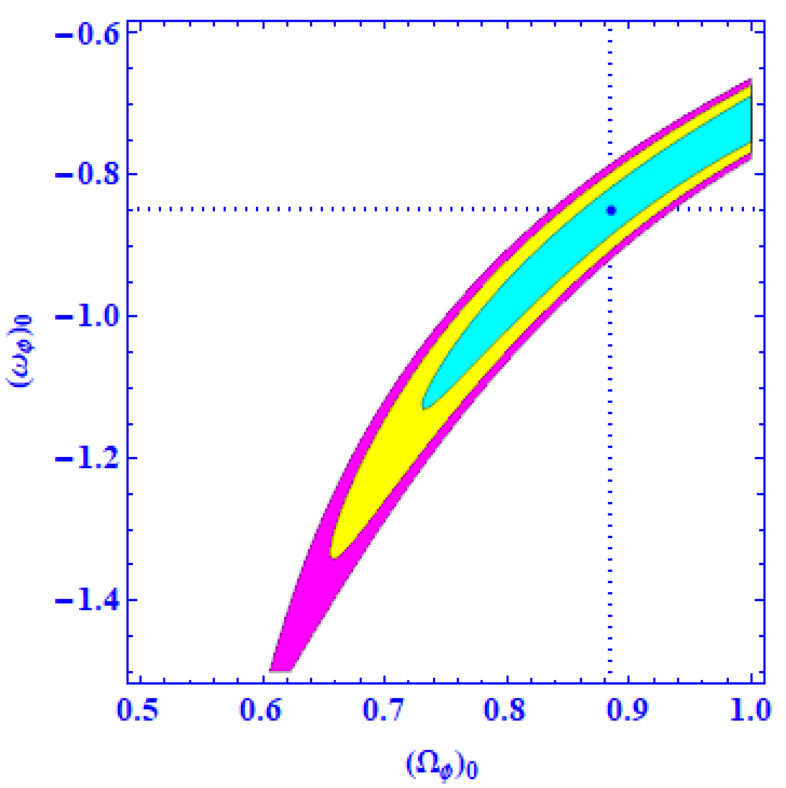
Figure 3.
Two-dimensional contours in the plane at , and confidence regions by bounding our model with joint and pantheon compilation of SN Ia data.
Figure 3.
Two-dimensional contours in the plane at , and confidence regions by bounding our model with joint and pantheon compilation of SN Ia data.

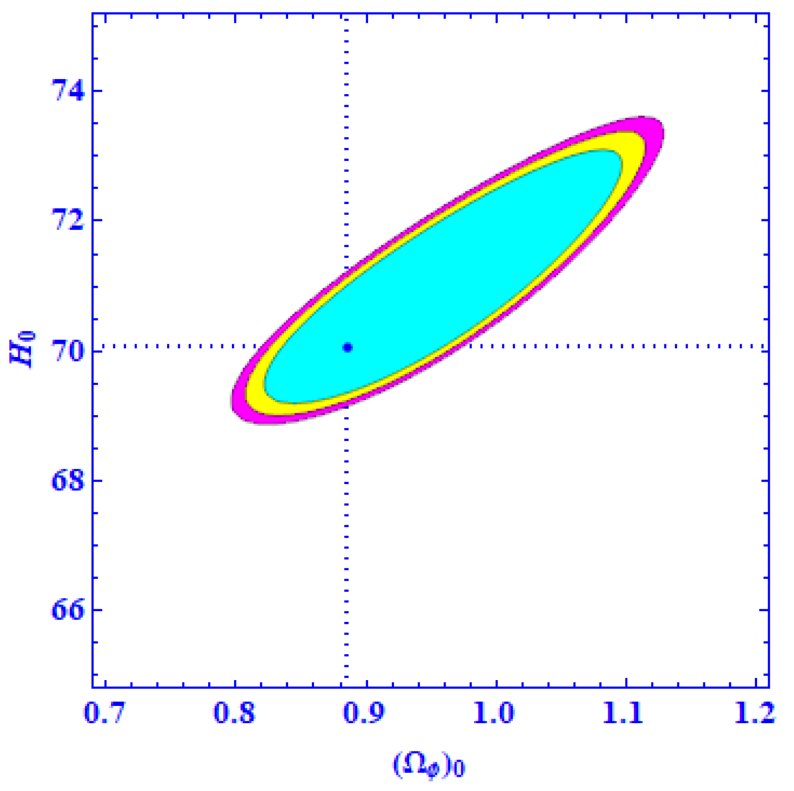
Figure 4.
Two-dimensional contours in the plane at , and confidence regions by bounding our model with joint and pantheon compilation of SN Ia data.
Figure 4.
Two-dimensional contours in the plane at , and confidence regions by bounding our model with joint and pantheon compilation of SN Ia data.

Figure 5.
Two-dimensional contours in the plane at , and confidence regions by bounding our model with joint and BAO data.
Figure 5.
Two-dimensional contours in the plane at , and confidence regions by bounding our model with joint and BAO data.

Figure 6.
Two-dimensional contours in the plane at , and confidence regions by bounding our model with joint and BAO data.
Figure 6.
Two-dimensional contours in the plane at , and confidence regions by bounding our model with joint and BAO data.

Figure 7.
Plot of versus redshift z.

Figure 8.
Variation of deceleration parameter versus redshift z for data (left panel, + Pantheon compilation of SN Ia data (middle panel) and + BAO data (right panel).
Figure 8.
Variation of deceleration parameter versus redshift z for data (left panel, + Pantheon compilation of SN Ia data (middle panel) and + BAO data (right panel).

Figure 9.
Single plot of q versus redshift z.

Figure 10.
Plot of r versus z.

Figure 11.
Plot of s versus z.

Figure 12.
Trajectory in the plane.

Table 1.
The BAO data points which we use in our analysis.
| S. N. | z | References | |
|---|---|---|---|
| 1 | 0.106 | 0.336 | [76] |
| 2 | 0.35 | 0.113 | [77] |
| 3 | 0.57 | 0.073 | [78] |
| 4 | 0.44 | 0.0916 | [79] |
| 5 | 0.60 | 0.0726 | [79] |
| 6 | 0.73 | 0.0592 | [17] |
Table 2.
Constrained values of model parameters.
| Parameters | + Pantheon | + BAO | |
|---|---|---|---|
Disclaimer/Publisher’s Note: The statements, opinions and data contained in all publications are solely those of the individual author(s) and contributor(s) and not of MDPI and/or the editor(s). MDPI and/or the editor(s) disclaim responsibility for any injury to people or property resulting from any ideas, methods, instructions or products referred to in the content. |
© 2023 by the authors. Licensee MDPI, Basel, Switzerland. This article is an open access article distributed under the terms and conditions of the Creative Commons Attribution (CC BY) license (https://creativecommons.org/licenses/by/4.0/).
Share and Cite
MDPI and ACS Style
Shrivastava, P.; Khan, A.J.; Kumar, M.; Goswami, G.; Singh, J.K.; Yadav, A.K. The Simplest Parametrization of the Equation of State Parameter in the Scalar Field Universe. Galaxies 2023, 11, 57. https://doi.org/10.3390/galaxies11020057
AMA Style
Shrivastava P, Khan AJ, Kumar M, Goswami G, Singh JK, Yadav AK. The Simplest Parametrization of the Equation of State Parameter in the Scalar Field Universe. Galaxies. 2023; 11(2):57. https://doi.org/10.3390/galaxies11020057
Chicago/Turabian StyleShrivastava, Preeti, Abdul Junaid Khan, Mukesh Kumar, Gopikant Goswami, Jainendra Kumar Singh, and Anil Kumar Yadav. 2023. "The Simplest Parametrization of the Equation of State Parameter in the Scalar Field Universe" Galaxies 11, no. 2: 57. https://doi.org/10.3390/galaxies11020057
Note that from the first issue of 2016, this journal uses article numbers instead of page numbers. See further details here.