
Refining Orbits of Bright Binary Systems
 , , , ,
Abstract
:1. Introduction
2. Previous Orbit Determinations for the Program Objects
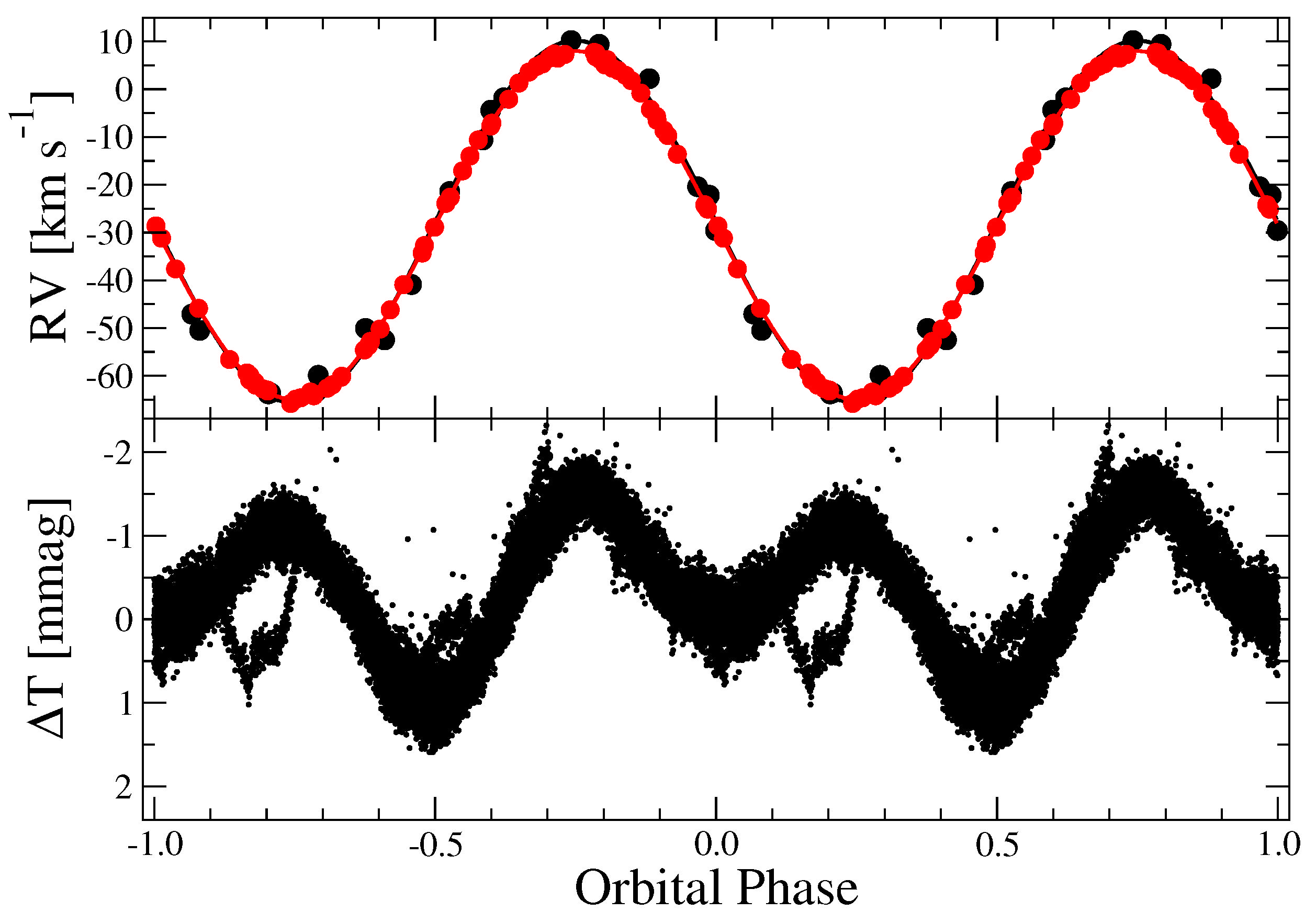
2.1. 02 UMa = HR 5055 = Mizar B

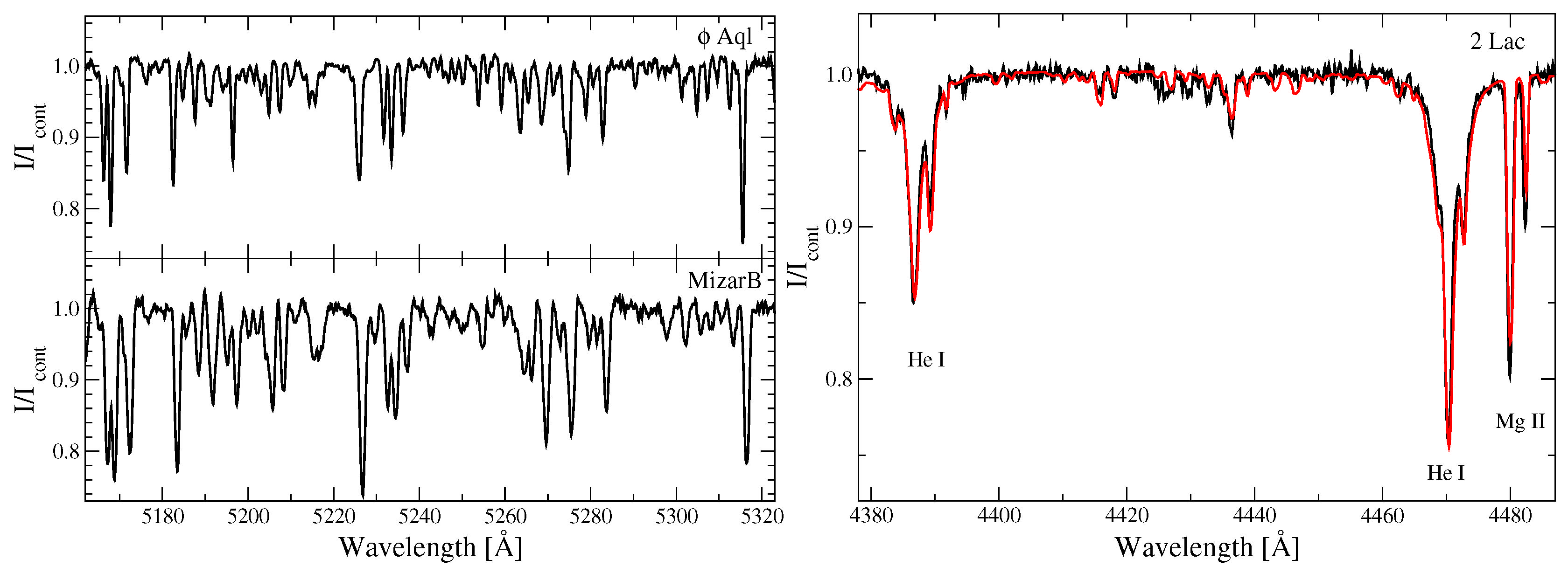
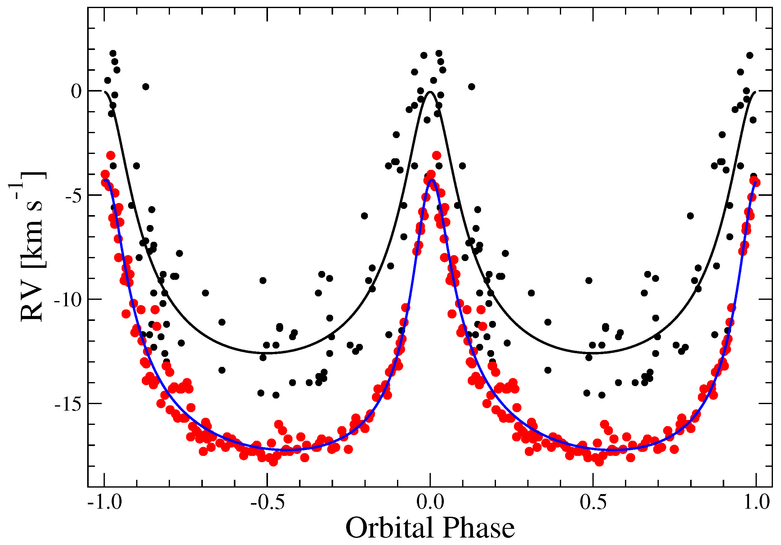
2.2. Aquilae = HR 7610
2.3. 2 Lacertae = HR 8523
3. Observations and Data Reduction
4. Results

| Element | [4] | [5] | TCO |
|---|---|---|---|
| P (days) | 361.24 | 175.55 ± 0.06 | 175.11 ± 0.10 |
| Epoch (HJD) | 2,417,623.68 | 2,437,294.4 ± 1.6 | 2,458,175.2 ± 0.7 |
| e | 0.697 | 0.46 ± 0.03 | 0.56 ± 0.09 |
| (degrees) | 27.14 | 4.3 ± 5.2 | 353.0 ± 4.6 |
| (km s) | −13.16 | ||
| K (km s) | 6.73 | 6.3 ± 0.2 | 6.46 ± 0.53 |
| f(m), M | 0.0042 | 0.0032 ± 0.0005 | 0.0028 ± 0.0011 |
| N | 24 | 89 | 155 |
| Element | [6] | [9] | TCO |
|---|---|---|---|
| P (days) | 3.320 ± 0.001 | 3.320680 | 3.320669 ± 0.000017 |
| T0 (JD) | 2,423,324.045 | 2,423,210.628 | 2,459,445.0916 ± 0.0011 |
| e | 0.055 ± 0.022 | 0 | 0 |
| (degrees) | 56.0 | − | − |
| (km s) | 0.63 | ||
| K (km s) | 38.25 ± 0.72 | 37.2 | 36.48 ± 0.07 |
| f(m), M | 0.019 ± 0.001 | 0.018 | 0.0167 ± 0.0001 |
| N | 34 | 30 | 80 |
| Element | [12] | Recalculation | TCO |
|---|---|---|---|
| P (days) | 2.616430 ± 0.000003 | 2.611523 ± 0.000004 | 2.616535 ± 0.000035 |
| T0 (HJD) | 242,700.80 ± 0.18 | 2,422,741.402 ± 0.011 | 2,459,423.7130 ± 0.0027 |
| e | 0.040 ± 0.018 | 0 | 0 |
| (deg) | 97.4 ± 25.3 | − | − |
| (km s) | |||
| K (km s) | 79.6 ± 1.8 | 72.78 ± 1.91 | 73.19 ± 0.47 |
| K (km s) | 100.0 ± 1.8 | − | 90.25 ± 0.71 |
| f(m), M | 0.137 ± 0.010 | 0.104 ± 0.007 | 0.106 ± 0.002 |
| f(m), M | 0.272 ± 0.015 | − | 0.199 ± 0.004 |
| N1/N2 | 82/61 | 135/63 | 42/29 |
| m, M | 0.87 ± 0.06 | − | 0.653 ± 0.021 |
| m, M | 0.69 ± 0.05 | − | 0.529 ± 0.018 |


5. Derivation of the Orbital Parameter Errors
6. Discussion
6.1. Error Comparison
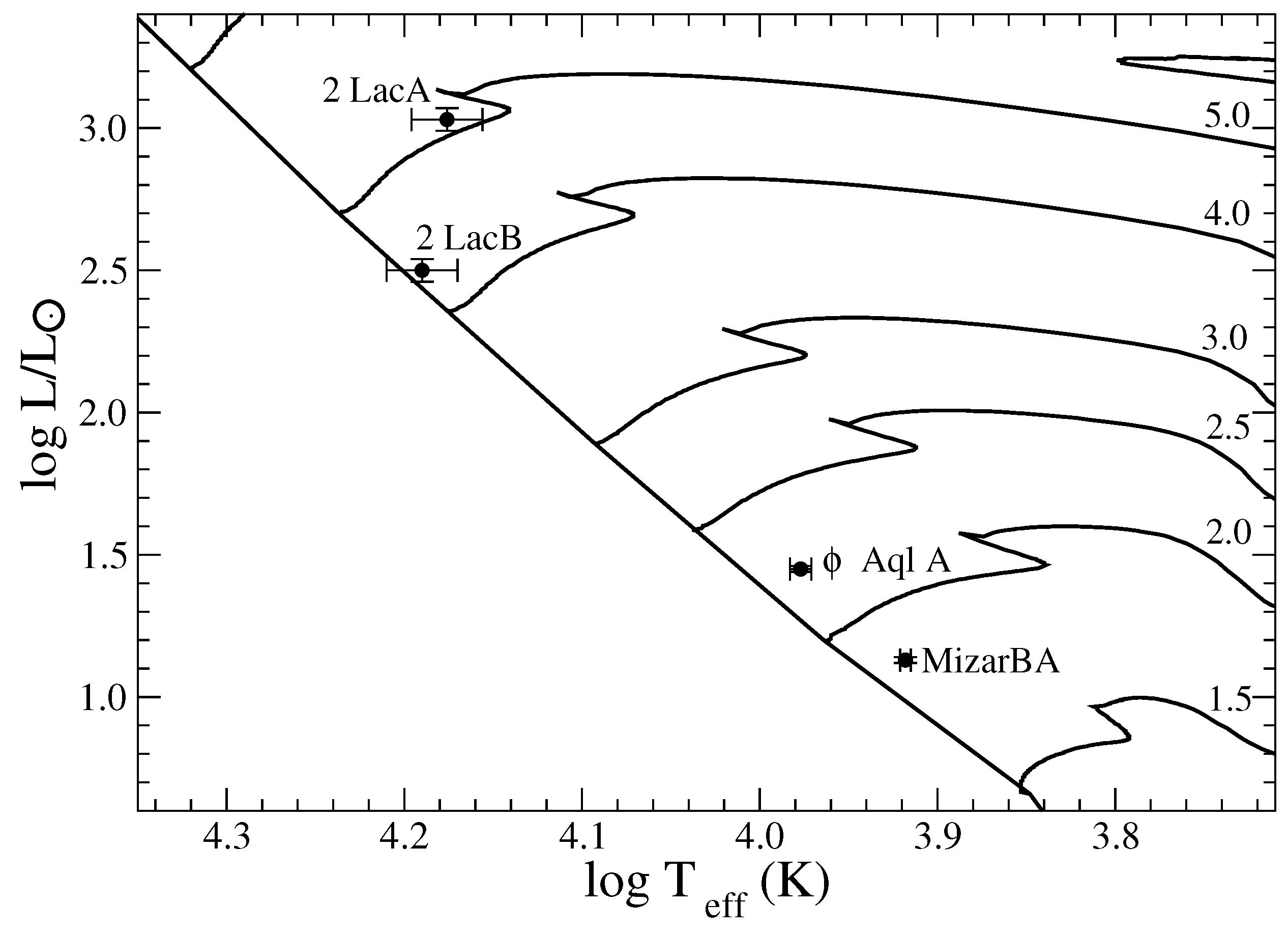
6.2. Fundamental Parameters
| Name | V–mag | D, pc | T, K | log L/L |
|---|---|---|---|---|
| MizarB | 3.91 | 24.81 ± 0.17 | 8279 ± 58 | 1.13 ± 0.01 |
| Aql | 5.28 | 67.67 ± 0.35 | 9484 ± 132 | 1.45 ± 0.01 |
| 2 Lac | 4.54 | 188.9 ± 6.0 | 13,996 ± 97 | 3.12 ± 0.04 |

6.2.1. Mizarb
6.2.2. Aql
6.2.3. 2 Lac
7. Conclusions
Author Contributions
Funding
Data Availability Statement
Acknowledgments
Conflicts of Interest
Abbreviations
| 1 | https://www.shelyak.com (accessed on 20 December 2022) |
References
- Preibisch, T.; Hofmann, K.H.; Schertl, D.; Weigelt, G.; Balega, Y.; Balega, I.; Zinnecker, H. Multiplicity of the young O- and B-type stars in the Orion Nebula cluster. IAU Symp. 2000, 200, 106. [Google Scholar]
- Dorn-Wallenstein, T.Z.; Levesque, E.M. Stellar Population Diagnostics of the Massive Star Binary Fraction. Astrophys. J. 2018, 867, 125. Available online: https://iopscience.iop.org/article/10.3847/1538-4357/aae5d6/pdf (accessed on 20 December 2022). [CrossRef] [Green Version]
- Frost, E.B. On certain spectroscopic binaries. Astron. Nachrichten 1908, 177, 171. [Google Scholar] [CrossRef] [Green Version]
- Abt, H.A. The Frequency of Binaries among Metallic-Line Stars. APJ Suppl. Ser. 1961, 6, 37–74. [Google Scholar] [CrossRef]
- Gutmann, F. The spectroscopic orbit of zeta1 Ursae Majoris (Mizar B). Publ. Dom. Astrophys. Obs. Vic. 1965, 12, 361–371. [Google Scholar]
- Harper, W. The Orbit of the Spectroscopic Binary phi Aquilae. Publ. Dom. Astrophys. Obs. Vic. 1922, 2, 179–182. [Google Scholar]
- Harper, W.H. Re-examination of 64 orbits. Publ. Dom. Astrophys. Obs. Vic. 1935, 6, 207–260. [Google Scholar]
- Batten, A.H. Sixth catalogue of the orbital elements of spectroscopic binary systems. Publ. Dom. Astrophys. Obs. Vic. 1967, 13, 119–251. [Google Scholar]
- Lucy, L.B.; Sweeney, M.A. Spectroscopic binaries with circular orbits. Astron. J. 1971, 76, 544–556. [Google Scholar] [CrossRef]
- Baker, R.H. The orbits of the spectroscopic components of 2 Lacertae. Publ. Allegh. Obs. Univ. Pittsburgh 1910, 1, 93–100. [Google Scholar]
- Luyten, W.J.; Struve, O.; Morgan, W.W. Reobservation of the orbits of ten spectroscopic binaries with a discussion of apsidal motions. Publ. Yerkes Obs. 1939, 7, 251–300. [Google Scholar]
- Hilditch, R.W. The binary systems 14 Cephei and 2 Lacertae. Mon. Not. R. Astron. Soc. 1974, 169, 323–329. [Google Scholar] [CrossRef]
- Usenko, I.A.; Kovtyukh, V.V.; Miroshnichenko, A.S.; Danford, S.; Prendergast, P. Pulsational activity changes in the Cepheid Polaris (α UMi) during 2017-2018: A new amplitude decrease. Mon. Not. R. Astron. Soc. 2018, 481, L115–L119. [Google Scholar] [CrossRef]
- Miroshnichenko, A.S.; Danford, S.; Zharikov, S.V.; Klochkova, V.G.; Chentsov, E.L.; Vanbeveren, D.; Zakhozhay, O.V.; Manset, N.; Pogodin, M.A.; Omarov, C.T.; et al. Properties of Galactic B[e] Supergiants. V. 3 Pup-Constraining the Orbital Parameters and Modeling the Circumstellar Environments. Astrophys. J. 2020, 897, 48. Available online: https://iopscience.iop.org/article/10.3847/1538-4357/ab93d9/pdf (accessed on 20 December 2022). [CrossRef]
- Stefanik, R.P.; Latham, D.W.; Torres, G. Radial-Velocity Standard Stars. In IAU Colloq. 170: Precise Stellar Radial Velocities; Hearnshaw, J.B., Scarfe, C.D., Eds.; Astronomical Society of the Pacific Conference Series; Astronomical Society of the Pacific: San Francisco, CA, USA, 1999; Volume 185, p. 354. [Google Scholar]
- Soubiran, C.; Jasniewicz, G.; Chemin, L.; Zurbach, C.; Brouillet, N.; Panuzzo, P.; Sartoretti, P.; Katz, D.; Le Campion, J.F.; Marchal, O.; et al. Gaia Data Release 2. The Catalogue of Radial Velocity Standard Stars. Astron. Astrophys. 2018, 616, A7. Available online: https://www.aanda.org/articles/aa/pdf/2018/08/aa32795-18.pdf (accessed on 20 December 2022). [CrossRef] [Green Version]
- Scargle, J.D. Studies in astronomical time series analysis. II. Statistical aspects of spectral analysis of unevenly spaced data. Astrophys. J. 1982, 263, 835–853. [Google Scholar] [CrossRef]
- Anderson, T.W. The Statistical Analysis of Time Series; Wiley: Hoboken, NJ, USA, 1994. [Google Scholar]
- Press, W.H.; Flannery, B.P.; Teukolsky, S.A. Numerical Recipes: The Art of Scientific Computing; Cambridge University Press: Cambridge, UK, 1986. [Google Scholar]
- Andronov, I.L. (Multi-) Frequency Variations of Stars. Some Methods and Results. Odessa Astron. Publ. 1994, 7, 49–54. [Google Scholar]
- Andronov, I.L. Advanced Time Series Analysis of Generally Irregularly Spaced Signals: Beyond the Oversimplified Methods. In Knowledge Discovery in Big Data from Astronomy and Earth Observation; Škoda, P., Adam, F., Eds.; Elsevier: Amsterdam, The Netherlands, 2020; pp. 191–224. [Google Scholar] [CrossRef]
- Efron, B.; Tibshirani, R.J. An Introduction to the Bootstrap; Chapman and Hall CRC: London, UK, 1993. [Google Scholar]
- Andrych, K.D.; Andronov, I.L.; Chinarova, L.L. MAVKA: Program of Statistically Optimal Determination of Phenomenological Parameters of Extrema. Parabolic Spline Algorithm And Analysis of Variability of The Semi-Regular Star Z UMa. J. Phys. Stud. 2020, 24, 1902. [Google Scholar] [CrossRef] [Green Version]
- Bailer-Jones, C.A.L.; Rybizki, J.; Fouesneau, M.; Demleitner, M.; Andrae, R. Estimating Distances from Parallaxes. V. Geometric and Photogeometric Distances to 1.47 Billion Stars in Gaia Early Data Release 3. Astrophys. J. 2021, 161, 147. Available online: https://iopscience.iop.org/article/10.3847/1538-3881/abd806/pdf (accessed on 20 December 2022). [CrossRef]
- Kornilov, V.G.; Volkov, I.M.; Zakharov, A.I.; Kozyreva, V.S.; Kornilova, L.N. Catalogue of four-colour WBVR magnitudes for 13586 northern sky objects. Tr. Gos. Astron. Instituta Sternberga 1991, 63, 4–399. [Google Scholar]
- Zorec, J.; Royer, F. Rotational Velocities of A-Type Stars. IV. Evolution of Rotational Velocities. Astron. Astrophys. 2012, 537, A120. Available online: https://www.aanda.org/articles/aa/pdf/2012/01/aa17691-11.pdf (accessed on 20 December 2022). [CrossRef] [Green Version]
- Miroshnichenko, A.S. New photometric calibration of the visual surface brightness method. IAU Symp. 1997, 189, 50. [Google Scholar]
- Ekström, S.; Georgy, C.; Eggenberger, P.; Meynet, G.; Mowlavi, N.; Wyttenbach, A.; Granada, A.; Decressin, T.; Hirschi, R.; Frischknecht, U.; et al. Grids of Stellar Models with Rotation. I. Models from 0.8 to 120 M⊙ at Solar Metallicity (Z = 0.014). Astron. Astrophys. 2012, 537, A146. Available online: https://www.aanda.org/articles/aa/pdf/2012/01/aa17751-11.pdf (accessed on 20 December 2022). [CrossRef] [Green Version]
- Pecaut, M.J.; Mamajek, E.E. Intrinsic Colors, Temperatures, and Bolometric Corrections of Pre-Main-Sequence Stars. APJ Suppl. Ser. 2013, 208, 9. Available online: https://iopscience.iop.org/article/10.1088/0067-0049/208/1/9/pdf (accessed on 20 December 2022). [CrossRef]
- De Rosa, R.J.; Patience, J.; Wilson, P.A.; Schneider, A.; Wiktorowicz, S.J.; Vigan, A.; Marois, C.; Song, I.; Macintosh, B.; Graham, J.R.; et al. The VAST Survey—III. The Multiplicity of A-Type Stars within 75 pc. Mon. Not. R. Astron. Soc. 2014, 437, 1216–1240. Available online: https://watermark.silverchair.com/stt1932.pdf?token=AQECAHi208BE49Ooan9kkhW_Ercy7Dm3ZL_9Cf3qfKAc485ysgAAAsowggLGBgkqhkiG9w0BBwagggK3MIICswIBADCCAqwGCSqGSIb3DQEHATAeBglghkgBZQMEAS4wEQQMbp-lxyEyh29HcxO3AgEQgIICfRUNCKtxFiAGGlcAxWQ–7T850L1l5gNR2MFg2KD7pH7uj-XaHGwyxdsSwQh68ZOYkD0tzkdT3wLMb0NND7K3T6zBK6AUZW-sftVTQq1t1JWEBjTO3WJa57mo_eTXchgwqwKlu7uuYYTCYvg2tpDCWu7eRMG73oMiklGCawcc4NVghrkICIACNJSAIlMtsuogPks7YSLyiRD3pVLPgEWNqMiTDPYkqY9vJQ1KeWxq2cI5syMrM-nRdLv8-gkC9jLMSnOKZ7AG9JvAZfGkWi3SmASGD0mdZsYNO_Oqu-_A7G_fAfRm5lb04BcolJGukriXS7cG87gGdBxwBYMkeh9s1b5hcImBpNsKjEc5mnpz5k01Mbe-aVsg01Wff9jUn-QhnZiBom17NFbxLCuisMov39dRZ7pE3WGhnruQlTz2v2Dn9bNaUH4hR2Bsf_8CGuEiPaVDdEf-jpoH_CUavkw6sndxn-_QpsUBdGEK9tu4IQSst8YjGz6fhrjYTlDIs0kOT0m3l_jTtQiBw7u6tginmozWhCdLLPMwI9HaSrfWccBKd8EEATPmRe54mqG9qm6kyIiyu-Qrc63mfBlfF2YBlnH7aM9y-3f4zy5VTYx0ft-Upth_ScZFqdNd0jw0xahAnXp8oWN0dI3LUSOYloDziGWRn-Df1vIeR423tkEq0Q9ud0yX4K8Tyzx6pG5S0MtftePLmRVgl_awGhWCB0Gt5cREtvItYb1qwLBcOKTEvxNSZzL3jHTx8x9LTaAGTGyYD4yypbtVchEts1vtHMlL2aahn8IIf6fGtL51plUpRNYlY7iWk_5r5cNEjChPs1w9AjX2228NEZLSMKCNVM (accessed on 20 December 2022). [CrossRef]
- Petrie, R.M. The determination of the magnitude difference between the components of spectroscopic binaries. Publ. Dom. Astrophys. Obs. Vic. 1939, 7, 205–238. [Google Scholar]
- Khokhlov, S.A.; Miroshnichenko, A.S.; Mennickent, R.; Cabezas, M.; Zhanabaev, Z.Z.; Reichart, D.E.; Ivarsen, K.M.; Haislip, J.B.; Nysewander, M.C.; LaCluyze, A.P. Toward Understanding The B[e] Phenomenon. VI. Nature and Spectral Variations of HD 85567. Astrophys. J. 2017, 835, 53. Available online: https://iopscience.iop.org/article/10.3847/1538-4357/835/1/53/pdf (accessed on 20 December 2022). [CrossRef] [Green Version]
- Zorec, J.; Cidale, L.; Arias, M.L.; Frémat, Y.; Muratore, M.F.; Torres, A.F.; Martayan, C. Fundamental Parameters of B Supergiants from the BCD System. I. Calibration of the (λ_1, D) Parameters into Teff. Astron. Astrophys. 2009, 501, 297–320. Available online: https://www.aanda.org/articles/aa/pdf/2009/25/aa11147-08.pdf (accessed on 20 December 2022). [CrossRef] [Green Version]
- Gray, R.O.; Corbally, C.J. The Calibration of MK Spectral Classes Using Spectral Synthesis. I. The Effective Temperature Calibration of Dwarf Stars. Astron. J. 1994, 107, 742. [Google Scholar] [CrossRef]
- Castelli, F.; Kurucz, R.L. New Grids of ATLAS9 Model Atmospheres. In Modelling of Stellar Atmospheres; Piskunov, N., Weiss, W.W., Gray, D.F., Eds.; Astronomical Society of the Pacific: San Francisco, CA, USA, 2003; Volume 210, p. A20. Available online: https://arxiv.org/pdf/astro-ph/0405087.pdf (accessed on 20 December 2022).
Disclaimer/Publisher’s Note: The statements, opinions and data contained in all publications are solely those of the individual author(s) and contributor(s) and not of MDPI and/or the editor(s). MDPI and/or the editor(s) disclaim responsibility for any injury to people or property resulting from any ideas, methods, instructions or products referred to in the content. |
© 2022 by the authors. Licensee MDPI, Basel, Switzerland. This article is an open access article distributed under the terms and conditions of the Creative Commons Attribution (CC BY) license (https://creativecommons.org/licenses/by/4.0/).
Share and Cite
Miroshnichenko, A.S.; Danford, S.; Andronov, I.L.; Aarnio, A.N.; Lauer, D.; Buroughs, H. Refining Orbits of Bright Binary Systems. Galaxies 2023, 11, 8. https://doi.org/10.3390/galaxies11010008
Miroshnichenko AS, Danford S, Andronov IL, Aarnio AN, Lauer D, Buroughs H. Refining Orbits of Bright Binary Systems. Galaxies. 2023; 11(1):8. https://doi.org/10.3390/galaxies11010008
Chicago/Turabian StyleMiroshnichenko, Anatoly S., Stephen Danford, Ivan L. Andronov, Alicia N. Aarnio, Duncan Lauer, and Holly Buroughs. 2023. "Refining Orbits of Bright Binary Systems" Galaxies 11, no. 1: 8. https://doi.org/10.3390/galaxies11010008