Tracing Hot Spot Motion in Sagittarius A* Using the Next-Generation Event Horizon Telescope (ngEHT)

Abstract

We propose the tracing of the motion of a shearing hot spot near the Sgr A* source through a dynamical image reconstruction algorithm, StarWarps. Such a hot spot may form as the exhaust of magnetic reconnection in a current sheet near the black hole horizon. A hot spot that is ejected from the current sheet into an orbit in the accretion disk may shear and diffuse due to instabilities at its boundary during its orbit, resulting in a distinct signature. We subdivide the motion into two different phases: the first phase refers to the appearance of the hot spot modeled as a bright blob, followed by a subsequent shearing phase. We employ different observational array configurations, including EHT (2017, 2022) and the next-generation Event Horizon Telescope (ngEHTp1, ngEHT) arrays, with several new sites added, and make dynamical image reconstructions for each of them. Subsequently, we infer the hot spot angular image location in the first phase, followed by the axes ratio and the ellipse area in the second phase. We focus on the direct observability of the orbiting hot spot in the sub-mm wavelength. Our analysis demonstrates that for this particular simulation, the newly added dishes are better able to trace the first phase as well as part of the second phase before the flux is reduced substantially, compared to the EHT arrays. The algorithm used in this work can be easily extended to other types of dynamics, as well as different shearing timescales. More simulations are required to prove whether the current set of newly proposed sites are sufficient to resolve any motions near variable sources, such as Sgr A*.

1. Modellng Flares in Sgr A* with Hot Spots

The recent resolved images of Sagittarius A* (Sgr A*) taken by the Event Horizon Telescope (EHT) [1,2,3,4,5,6,7,8,9,10] revealed rapid structural variability in the resolved supermassive black hole (SMBH) source at the galactic center [11,12]. These findings complement the reported variability in this compact source across the electromagnetic spectrum [13], in the mm/sub-mm scale [8,14,15,16,17,18,19,20,21], in  near-infrared (NIR) [22,23,24], and in X-rays [25,26,27,28,29,30]. Later work found evidence for an NIR and sub-mm correlation and a possible adiabatic expansion of the emitting region during a flare [13,31,32,33,34,35]. During flare events, the flux density observed in NIR and X-rays increases by 1-2 orders of magnitude, which roughly aligns with theoretical expectations, e.g., [36]. The flares seem to originate from a compact region near the innermost stable circular orbit (ISCO) [37,38]. In particular, ref. [38] recently reported an orbiting hot spot detection in the unresolved light curve data at the EHT observing frequency following an X-ray flare.

On the theoretical front, there have been various explorations trying to model these flares (hot spots) in a general relativistic magnetohydrodynamical (GRMHD) framework or through semi-analytic models. In the former case, magnetic reconnection and the flux eruption [36,39] are good candidates to produce such flares in a form of a hot spot region orbiting around the SMBH, arising from the local energy injection accelerating the electrons within the accretion disk. In the latter case [40,41,42,43,44], the hot spot may be embedded within a geometrically thick, hot, and optically thin, radiatively inefficient accretion flow (RIAF; [45,46,47,48]), expected to be characteristic of low-luminosity SMBHs such as Sgr A*.

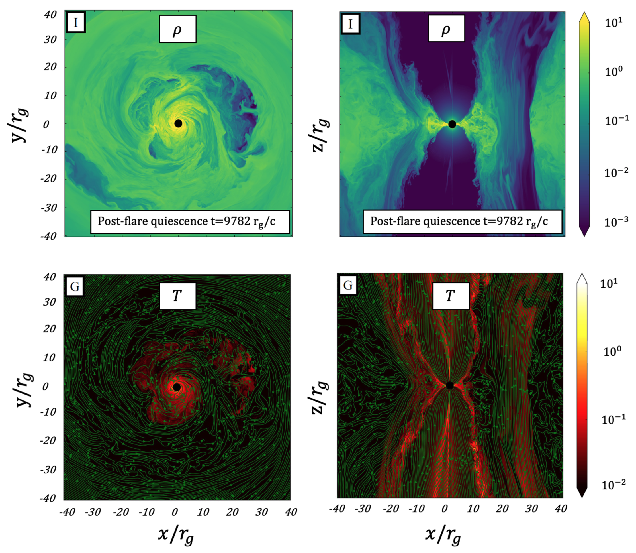
2. Dynamical Formation of a Hot Spot in the Simulations

The formation of hot spots has been reported in general relativistic magnetohydrodynamics (GRMHD) simulations. In these simulations, as the gas near the black hole becomes more magnetized, reaching the magnetically arrested disk (MAD; [49]) state, horizontal fields squeeze the accretion flow, thereby forming a thin equatorial current sheet [50]. This current sheet is potentially unstable to tearing instabilities and the formation of plasmoids via reconnection. Plasmoids are blobs of plasma confined by a helical field, consisting of particles energized by the reconnection of the surrounding magnetized plasma.

In a scenario proposed by [50], an equatorial reconnection layer transforms the horizontal field at the jet base into a vertical field that is injected into the accretion disk. The flux tube of the vertical field is filled with non-thermal leptons originating from the jet’s magnetized plasma and accelerated by the reconnection event. The resulting low-density hot spot, is contained by the vertical magnetic field and subsequently orbits around the black hole and is conjectured to power the NIR emission trailing a large X-ray flare. Figure 1 presents the dynamical formation of the hot spot filled with low-density plasma contained by vertical field from a HAMR simulation (using a GPU-accelerated and advanced custom-built adaptive mesh refinement (AMR) code) [50,51]. In Figure 1, $\rho$ and T refer to the mass density and the temperature, respectively.

Large plasmoids, formed due to mergers of smaller plasmoids in reconnection layers, have also been conjectured as a model for orbiting hot spots. The growth and propagation of plasmoids is still an ongoing area of research, especially in full 3D GRMHD. Because of the potential of these plasmoids to carry non-thermal electrons (as magnetic reconnection can drive particle acceleration), several works have tried to model plasmoid evolution as spherical or shearing hot spots around black holes [42,43,52,53,54,55,56,57].

The main difference between the vertical flux tube scenario and an individual large plasmoid as a hot spot model is twofold: a plasmoid consists of a dominantly helical field and is shown to mainly orbit along the jet sheath [58,59], whereas a large flux tube formed as reconnection exhaust consists of a vertical field and orbits in the accretion disk. Recent observations of orbiting hot spots suggest a dominant vertical field component [37,38] associated with the motion, which implies that a vertical field flux tube may be more realistic as the source of emission instead of a large individual plasmoid. On the other hand, in a different scenario, an apparent hot spot observed at mm wavelengths could correspond simply to a local density maximum, possibly originating in the turbulent accretion flow or related to an infalling clump of matter [60].

3. Semi-Analytic Simulation of a Shearing Hot Spot

There have been a variety of different hot spot models. The original studies [40,41,42] only focused on the coherent motion of a spherical Gaussian hot spot. Others [34] extended this model by adding the adiabatic expansion and [61] considered a 2D shearing hot spot, ignoring the radiative transfer effects. More recently, ref. [43] extended this model further and included both the shearing and the expansion of a 3D hot spot, additionally incorporating polarized radiative transfer effects such as absorption and Faraday rotation, while ref. [44] focused on employing a full polarized radiative transfer to the coherent Gaussian hot spot model. To describe shearing and expansion, ref. [43] assumes that the hot spot electron number density follows the continuity equation and travels along a prescribed velocity field $u^{\mu }$. To make the solution to the continuity equation tractable, the velocity field is restricted to have no vertical motion, be stationary, and be axisymmetric with respect to the spin axis. Given these restrictions, the continuity equation describing the electron number density $n_e$ can be solved semi-analytically using the equation [43]:

$$n_e(\tau ,x^{\mu })=n_{e0}\left(y^{\mu }\right)\frac{u^r\left(y^{\mu }\right)}{u^r\left(x^{\mu }\right)}\times \sqrt{\frac{g\left(y^{\mu }\right)}{g\left(x^{\mu }\right)}},$$

(1)

where $n_{e0}\left(y^{\mu }\right)$ refers to the initial proper density of a hot spot, $y^{\mu }$ describes its initial location, $x^{\mu }$ refers to its subsequent position, and $g\left(x^{\mu }\right)$ denotes the metric tensor determinant evaluated at the location $x^{\mu }$. Note that $y^{\mu }={\varphi }_{-\tau }\left(x^{\mu }\right)$, where ${\varphi }_{\tau }$ is the velocity field flow found by integrating ${\dot{x}}^{\mu }=u^{\mu }$ for $\tau$ units of proper time. For this work, we used the hot spot simulation from [62], representing an orbiting feature around a black hole with a spin of 0.1 and an inclination of ${160}^{\circ }$. The hot spot was initialized in the equatorial plane at a radius of $7M$ with a Gaussian profile with a full-width-half-max (FWHM) of $1.18M$. We used the semi-analytical RIAF model from [63], with a Keplerian velocity field to represent the quiescent background accretion flow. We note that the hot spot parameters used are consistent with the constraints provided by [37,38].

Figure 2 presents the appearance of the shearing hot spot at a few different times in the image space (top row) and in the visibility space using EHT2017, EHT2022, phase I of ngEHT (ngEHTp1), and the full ngEHT array (ngEHT), respectively.

In this paper, we will analyze how well different EHT/ngEHT arrays are able to dynamically reconstruct hot spot motion from Figure 2 using the StarWarps algorithm [64] (see below for more details). To accomplish this analysis, we perform synthetic observations using four different observational array configurations. These configurations include both of the current EHT coverage (EHT2017, EHT2022), as well as the next-generation Event Horizon Telescope (ngEHT) arrays (ngEHTp1, ngEHT), see

Table 1. Array configurations used for EHT and ngEHT coverage and simulated data sets. The Greenland Telescope (GLT) is part of the EHT array (from 2018 onwards), but has not been used in our simulations since it is too far north to observe Sgr A*. ngEHT configurations assume the participation of existing EHT (2022) sites, as well as the addition of existing/repurposed dishes at HAY (37 m), OVRO (10 m), and GAM (15 m), or hypothetical 6m dishes at new site locations. On-sky bandwidth is assumed to be 4 GHz for EHT(2017), 8 GHz for EHT(2022), and 16 GHz at both 230 and 345 GHz for ngEHT. The ngEHT Phase 1 and 2 station acronyms relate to nearby observatories or geographical locations: Owens Valley Radio Observatory in California, USA (OVRO); Haystack Observatory in Westford, MA, USA; La Palma, part of the Canary Islands, Spain (CNI); National Astronomical Observatory in Baja California, Mexico (BAJA); Las Campanas Observatory in Chile (LAS); the German Antarctic Receiving Station O’Higgins in Antarctica (GARS); the Gamsberg in Namibia (GAM); Cerro Catedral in R’io Negro in Argentina (CAT); the La Paz region in Bolivia (BOL); and the Espírito Santo region in Brazil (BRZ). See [65] for more site details and locations on a map.

Array	Sites Used for Simulated Data
EHT(2017)	ALMA	APEX	SMA	JCMT	SMT	LMT	PV	SPT
EHT(2022)	EHT(2017)+	KP	NOEMA
ngEHTp1	EHT(2022)+	OVRO	HAY	CNI	BAJA	LAS
ngEHT	ngEHTp1+	GARS	GAM	CAT	BOL	BRZ

.

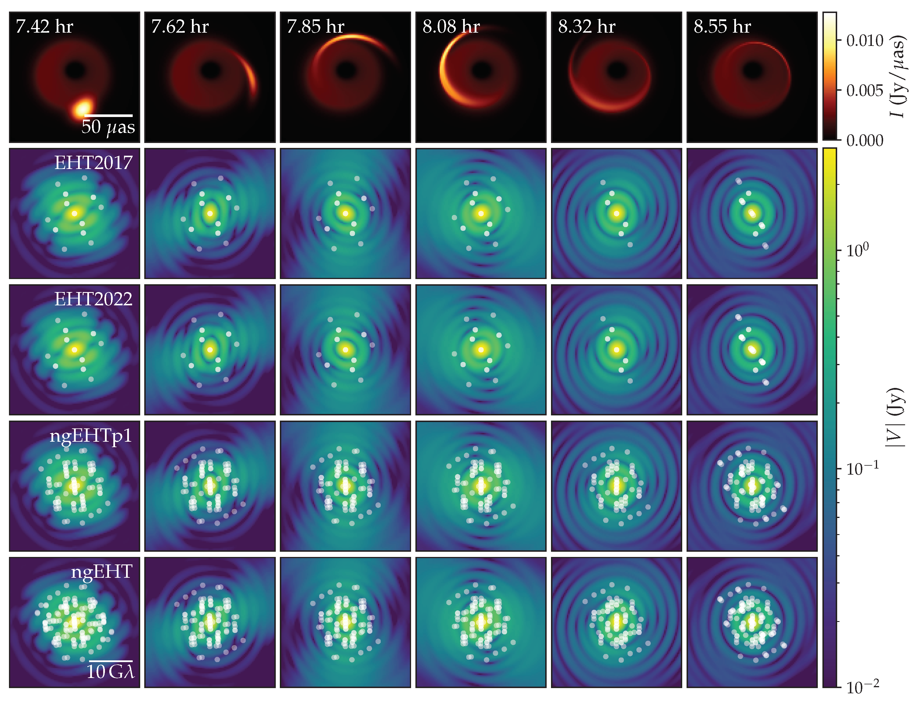
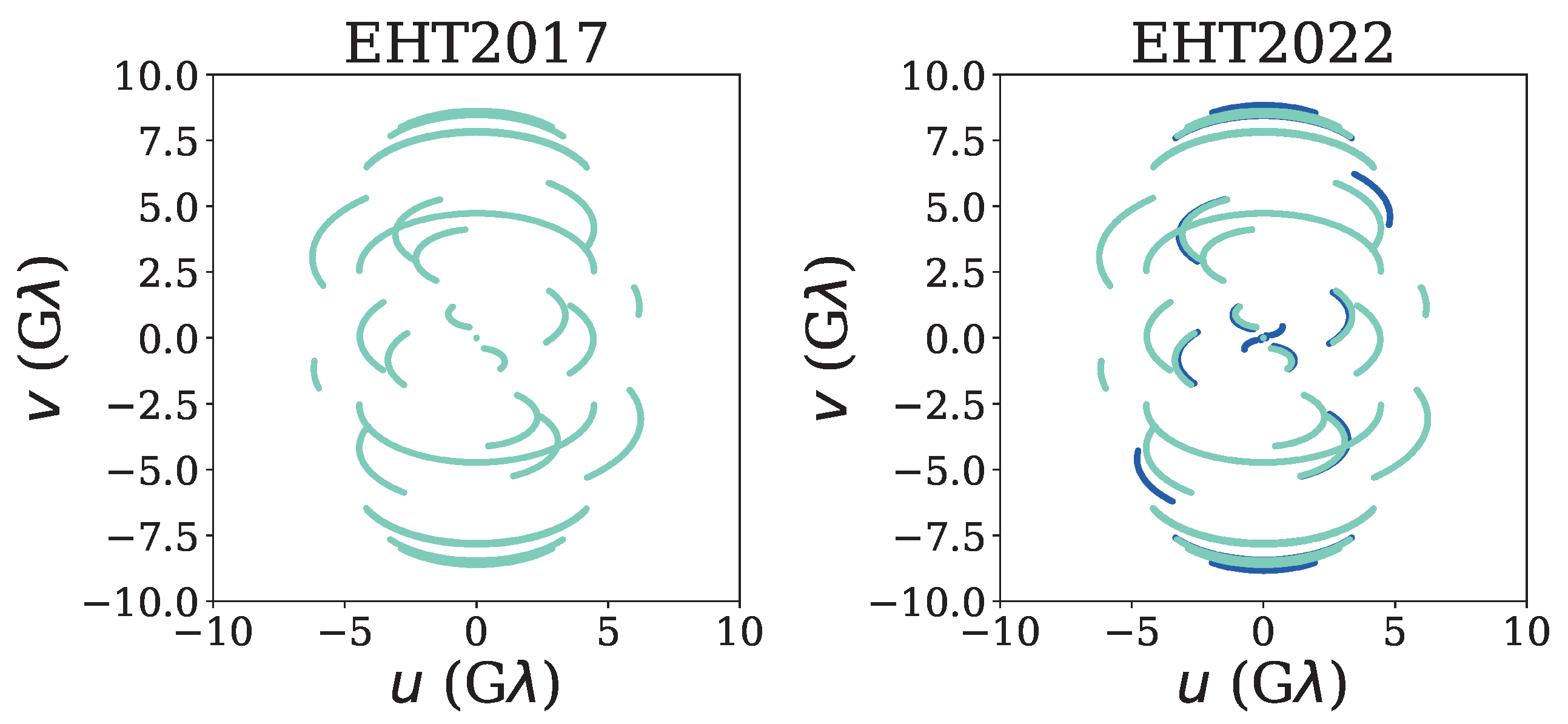
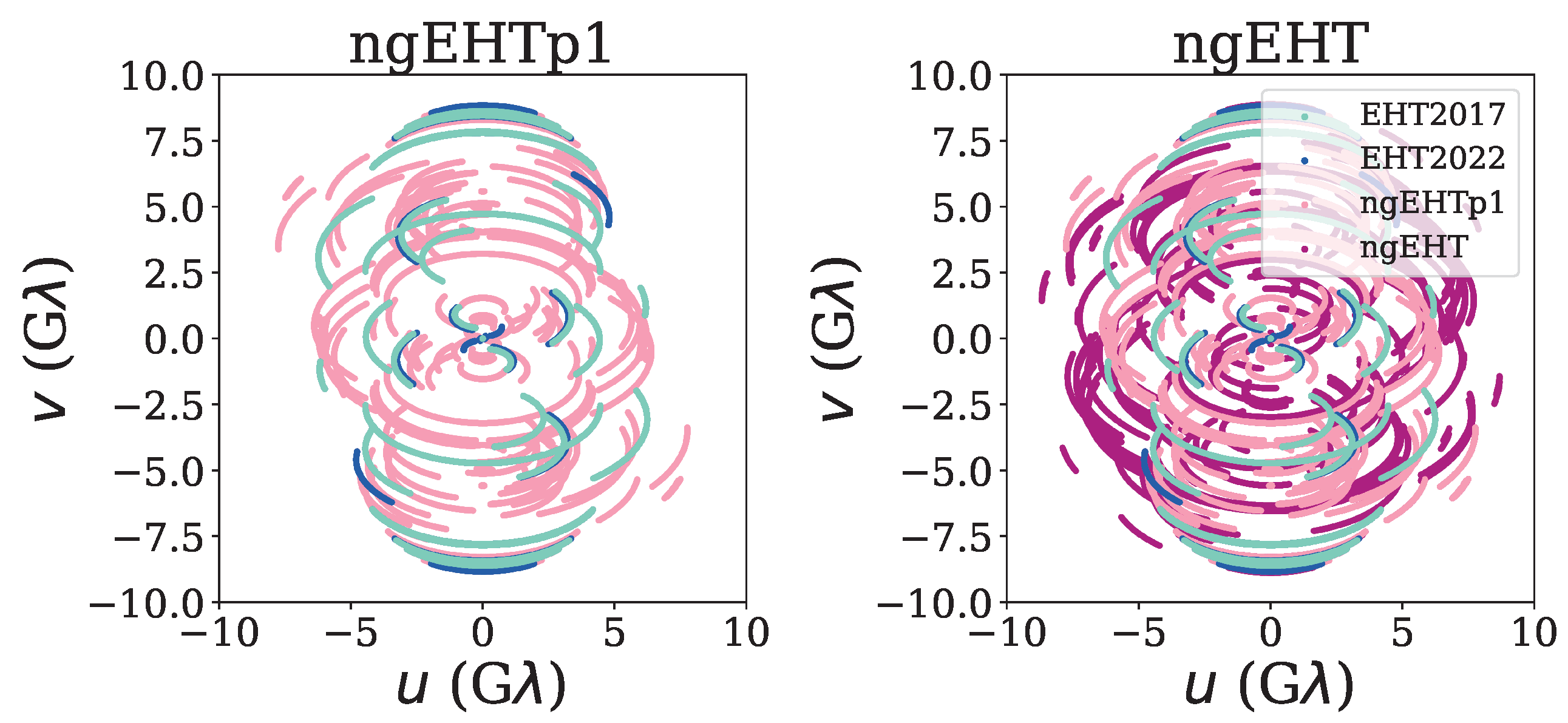
4. Creating Synthetic Data for EHT/ngEHT

To make the synthetic data for the dynamical image reconstruction, we used the eht-imaging package [66,67,68].

We consider four different array configurations, including the EHT(2017), EHT(2022), ngEHTp1, and ngEHT. Representative April weather is used to simulate station performance, along with random (uncalibrated) absolute atmospheric phase and ∼10% amplitude gain systematic error. Table 1 contains a list of stations used for each array configuration.

Before generating the synthetic data, we scatter the movie frames using the interstellar scattering model for Sgr A* from [69], as implemented in eht-imaging. Figure 3 presents the uv-coverage of the above arrays. The top row presents the EHT2017 (left panel) and EHT2022 (right panel) uv-coverage, while the bottom row shows the uv-coverage for ngEHTp1 (left panel) and ngEHT (right panel), respectively.

5. Dynamical Reconstruction Using the  StarWarps Code

Since the gravitational time scale for Sgr A* is $t_g=GM/c^3\simeq$ 20 sec, the image structure varies greatly throughout an observation. Consequently, the static image assumption [4] breaks down, making the standard imaging approaches inadequate. Constructing a time variable image is further complicated by the fact that as the image changes, so does the telescope, due to the rotation of the Earth. Therefore, any dynamical imaging algorithm needs to disentangle the coverage evolution from the dynamical evolution of the source. To solve this problem, we use StarWarps [64]. StarWarps is a novel dynamical imaging algorithm that models the Very Long Baseline Interferometry (VLBI) observations using a Gaussian Markov Model to model the image variability. By using a specific model for the variability StarWarps is able to simultaneously reconstruct both the image and its motion, allowing the algorithm to disentangle the variations due to the telescope from the image itself. In more detail, StarWarps reconstructs an N-dimensional (hereafter referred to as N-D) image vector $X=\{x_1,x_2,\cdots ,x_N\}$, where N denotes the total number of unique timestamps of the observation and $x_t$ is a flattened vector of the image pixel intensities. The data vector $Y=\{y_1,y_2,\cdots ,y_N\}$ is given by the sparse interferometric measurements for the telescope. Note that each snapshot of data $y_t$ may itself be a vector since each timestamp typically has many different telescopes observing the source. The StarWarps dynamical imaging model is given in terms of the following potentials, $\phi$:

$$\begin{array}{cc}\hfill {\phi }_{y_t|x_t}& ={\mathcal{N}}_{y_t}(f_t\left(x_t\right),R_t),\hfill \end{array}$$

(2)

$$\begin{array}{cc}\hfill {\phi }_{x_t}& ={\mathcal{N}}_{x_1}({\mu }_t,{\Lambda }_t),\hfill \end{array}$$

(3)

$$\begin{array}{cc}\hfill {\phi }_{x_t|x_{t-1}}& ={\mathcal{N}}_{x_t}(A{x}_{t-1},Q),\hfill \end{array}$$

(4)

where $\mathcal{N}(x,\Sigma )$ denotes a multivariate Gaussian with mean $\mu$ and covariance $\Sigma$. The potential ${\phi }_{y_t|x_t}$ is given by the likelihood of the problem, where $f_t$ denotes the function that transforms from the image pixel intensities $x_t$ to the observed data products $y_t$. The covariance $R_t$ is given by the thermal noise from the telescope, plus an additional systematic factor, which we discuss below.

The potential ${\phi }_{x_t}$ denotes the image prior, where we set ${\Lambda }_t=\mathrm{diag}{\left[{\mu }_t\right]}^T{\Lambda }^{\prime }\mathrm{diag}\left[{\mu }_t\right]$ to ensure that the image intensities are positive. The mean image ${\mu }_t$ is typically chosen to be a simple image (e.g., a ring) whose structure depends on the problem. We specify the $\mu$ and $\Lambda$ we use below.

Finally, ${\phi }_{x_t|x_{t-1}}$ specifies the dynamical aspects of the model. To describe the dynamic, StarWarps breaks it down into two separate components: a fixed global variability plus a correlated stochastic piece. The fixed global variability is given by the matrix A and specifies a constant linear evolution of the problem. If A is the identity matrix, then there is no global evolution; instead, all dynamics are given by the second stochastic part. To describe the stochastic evolution, StarWarps assumes that the $x_t=x_{t-1}+\epsilon$, where $\epsilon$ is drawn from a multivariate Gaussian with zero mean and covariance Q. This model thus describes a linear evolution of the image I with correlated fluctuations that can additionally modify the image. Note that StarWarps reduces to static imaging when A is the identity matrix and $Q=0$. For simplicity, we set $A=\mathrm{𝟙}$, the identity matrix, and leave exploring the impact of non-trivial A to future work.

By multiplying these three potentials together, we can form the Joint distribution of StarWarps as:

$$p(X,Y;A=\mathrm{𝟙})\propto \prod _{t=1}^N{\phi }_{y_t|x_t}\prod _{t=1}^N{\phi }_{x_t}\prod _{t=2}^N{\phi }_{x_t|x_{t-1}}.$$

(5)

StarWarps solves for N-D image array $X={\left\{x_t\right\}}_t$ by using the N-D observed data points $Y={\left\{y_t\right\}}_t$. Recall that $f_t,R_t$ are known from the data, while ${\mu }_t,{\Lambda }_t$, and Q are hyperparameters of the model.

For our reconstructions, we used the bispectrum (bs), log closure amplitude (logcam), and closure phase (cphase) as the data products. In addition to the thermal noise of the telescope for a baseline i, ${\sigma }_i$, we include an additional error budget equal to 2% of the visibility amplitudes added in quadrature:

$${\sigma }_i^2\to {\sigma }_i^2+{\left(0.02\right)}^2{\left|V_i\right|}^2$$

(6)

where $V_i$ is the measured visibility for baseline i. This additional error is added to capture the expected magnitude of the unknown systematic errors (e.g., related to averaging over a wide frequency band or resulting from imperfect polarimetric leakage calibration), see [2]. In addition, we include a set of weights $w^{\left(i\right)}$ for each data product that effectively modifies the covariance $R_t^{\left(i\right)}\to {\left(w^{\left(i\right)}\right)}^{-1}{R}_t^{\left(i\right)}$ for each data product i.

Table 2. Down rows present the data terms as well as different ${\chi }^2$s for the quality of the reconstructed images using StarWarps for different arrays. From top to bottom, we present EHT(2017), EHT(2022), ngEHTp1, and the full ngEHT. Bs, logcam, and cphase refer to the data weights associated with the bs, log closure amplitude, and the closure phase, respectively.

Obs	Bs	logcam	cphase	${\mathit{\chi }}_{\mathbf{cphase}}^2$	${\mathit{\chi }}_{\mathbf{logcamp}}^2$	${\mathit{\chi }}_{\mathbf{camp}}^2$
EHT(2017)	1.0	1.0	1.0	0.67	1.16	1.37
EHT(2022)	1.0	1.4	1.7	0.59	0.63	0.77
ngEHTp1	1.2	1.5	1.5	1.14	1.5	1.84
ngEHT	1.0	1.0	1.0	1.17	1.51	1.90

gives the weights for each data product.

We set our prior image, $\mu ={\mu }_t$, to be an infinitely thin ring with the typical diameter of Sgr A*, which is then blurred with a 25 $\mu$ as FWHM. To specify ${\Lambda }^{\prime }$, we follow the procedure in [64] and define it using a power spectrum P given by:

$$P(u,v)=\frac{c_0{ϵ}^a}{{(u^2+v^2+ϵ)}^a},$$

(7)

where $a=0.3$, $c_0=0.3$, and $ϵ={10}^{-3}$. ${\Lambda }^{\prime }$ is then equal to the Fourier transform of Equation (7). Finally, we set $Q={\beta }_Q\mathrm{𝟙}$, where ${\beta }_Q=5\times {10}^{-6}$.

6. Reconstructing the Motion of the Hot Spot in Different Arrays

Here, we use the StarWarps code to make a dynamical image reconstruction of the orbiting hot spot using different observational arrays. Table 2 presents the ${\chi }^2$ of different arrays. In this paper, we focus on the improvements in movie reconstructions using different EHT/ngEHT array configurations, and future work will focus on improving various StarWarps hyperparameters, as well as considering different simulations.

Figure 4 compares the original hot spot with the reconstructed images from different arrays at few time snapshots. Down rows correspond to different times, while different columns (from left to right) show the original hot spot, EHT(2017), EHT(2022), ngEHTp1, and ngEHT, respectively. It is generally seen that the ngEHT arrays are doing a better job at reconstructing the hot spot’s motion. However, the quality of the reconstructed images reduces around T = 7.62 UT when the hot spot moves behind the source, leading to a flux reduction.

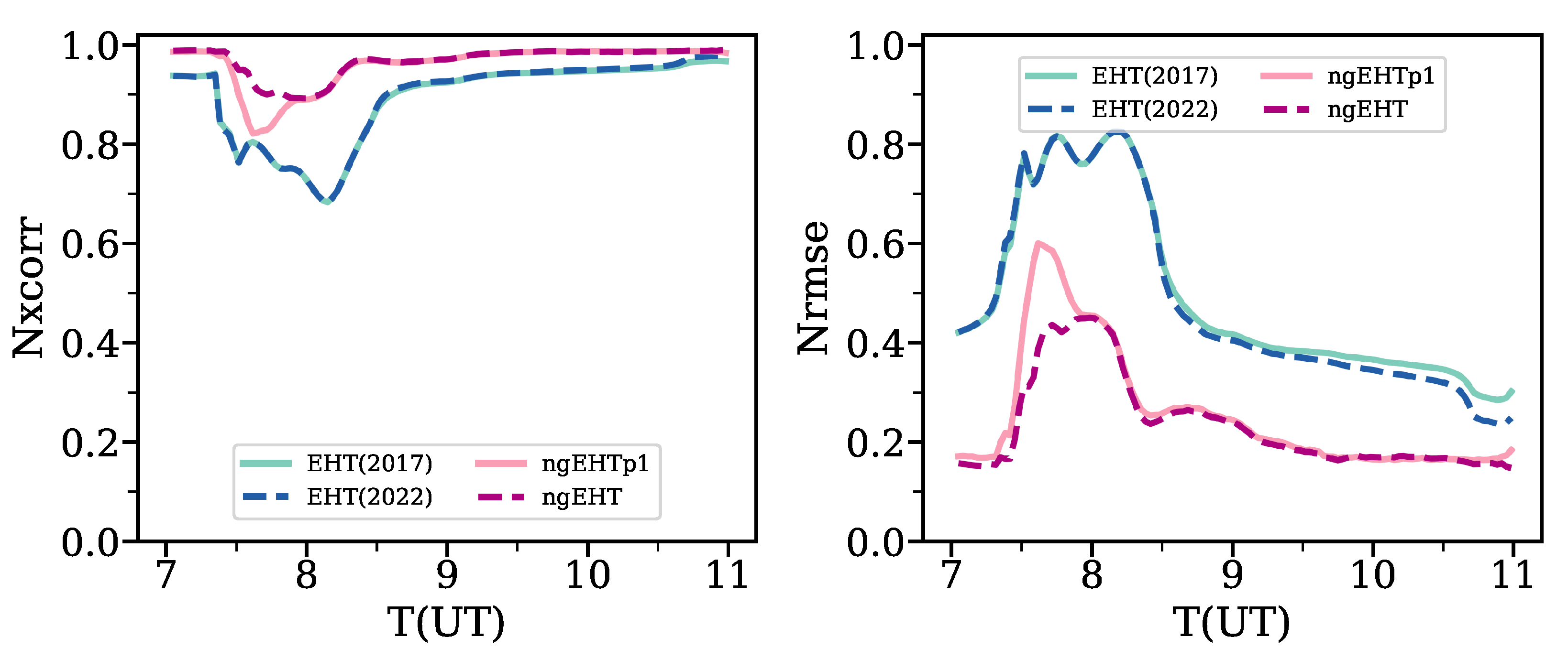
Nxcorr vs. Nrmse of the Reconstructed and Ground Truth Image

To make a more quantitative comparison between the reconstructed and the ground truth images, here we infer the normalized cross-correlation (hereafter $\mathrm{Nxcorr}$), as well as the normalized root-mean-squared error (hereafter $\mathrm{Nrmse}$), between the reconstructed image and its ground truth image:

• $\mathrm{Nxcorr}$: We make use of [67,70], defining the $\mathrm{Nxcorr}$ as:

  $$\mathrm{Nxcorr}(X,Y)=\frac{1}{N}\sum _i\frac{\left(X_i-\langle X\rangle \right)\left(Y_i-\langle Y\rangle \right)}{{\sigma }_X{\sigma }_Y},$$

  (8)

  where X refers to the restructured image, while Y describes the ground truth image of the hot spot. Furthermore, N stands for the number of the pixels in the image, and $\langle \rangle$ refers to the mean pixel value of the image. Finally, ${\sigma }_i$ describes the standard deviation of pixel values in image i. $\mathrm{Nxcorr}$ determines the similarities between two images. A perfect correlation between the images leads to 1, while a complete anti-correlation between them gives rise to a value of −1 for $\mathrm{Nxcorr}$.
• $\mathrm{Nrmse}$ is defined as [67]:

  $$\mathrm{Nrmse}=\frac{{\sum }_i{|X_i-Y_i|}^2}{{\sum }_i{\left|X_i\right|}^2}.$$

  (9)

  where, unlike the case of $\mathrm{Nxcorr}$, two completely similar (different) images X and Y have 0 (1) value $\mathrm{Nrmse}$.

Figure 5 presents the $\mathrm{Nxcorr}$ and $\mathrm{Nrmse}$ for reconstructed images computed using different arrays. From the plot, it is inferred that:

∘

Since the background RIAF is dominated in some snapshots, it is seen that we have a globally good correlation between the images.

∘

This, however, becomes worse when the hot spot appears and becomes sheared down, in which it is seen that we have a some levels of suppression (enhancement) of $\mathrm{Nxcorr}$ ($\mathrm{Nrmse}$) for some cases.

∘

The aforementioned suppression (enhancement) is, however, minimal for the ngEHT array compared with the EHT(2017) and EHT(2022).

∘

Consequently, we conclude that the ngEHT array helps a lot in improving the quality of the reconstructed image.

7. Tracking the Angular Location of the Hot Spot

The motion of a shearing hot spot can be subdivided to two distinct phases. The first phase corresponds to a bright (compact) blob that initially appears and starts orbiting around the black hole. The first phase occurs initially up to 7.65 UT. From 7.65 UT and onward, the hot spot is in the second phase, where the hot spot shears out along the differentially rotating velocity field. We use two distinct metrics to trace these distinct evolution phases.

• First phase (<7.65 UT): In phase 1, due to the hot spot’s compact nature, we track the peak intensity I divided by the initial intensity $I_0$ of either the original hot spot or the reconstructed intensity for the reconstructed movies. Furthermore, we also follow the peak intensity’s angular location $\Phi$.

Figure 6 compares the time evolution of the normalized peak intensity (top row), as well as the angular location of the intensity maximum, referred (bottom row) between the original hot spot (black solid line) and the reconstructed values from different observational arrays during the first phase of evolution. This includes EHT2017 (cyan solid line) and EHT2022 (dashed blue line) arrays (left panel), as well as the ngEHTp1 (pink solid line) and ngEHT (dashed magenta line) arrays (right panel), respectively. Note that to make the figure, we smoothed each curve with a Gaussian filter with a $4\mathrm{mins}$ standard deviation. From the plot, it is inferred that the reconstructed shape of the intensity and the phase are closer to the original hot spot for ngEHT arrays compared with the EHT ones. Furthermore, in the phase plot on the bottom row, it is seen that in original time the phase is very close to the original hot spot, where the level of agreement is higher in ngEHT arrays than the EHT ones.

• Second phase (>7.65 UT): To extract the hot spot motion in the second phase, we model it as a stretched ellipse and infer its axes ratio as well as the ellipse area over time. Since the background is dominated by the RIAF model, to extract the ellipsoidal motion, in each snapshot, we first find out the points with an intensity above 80% of the intensity max on that snapshot. We then compute the ellipticity as $(\mathrm{b}/\mathrm{a})$, where a and b are the associated semi-major and semi-minor ellipse axes, respectively. The ellipse area is then estimated as $\pi ab$.

Figure 7 presents the time evolution of the ellipticity (top row) and the ellipse area (bottom row) using different observational arrays. Overlaid on the plot, we also show the corresponding values for the hot spot model (black lines). To make the plot more readable, we first smooth all the curves using a Gaussian filter with a standard deviation of $4\mathrm{mins}$. For each data set, we show two curves. The higher-transparency curve is just the value from the smoothed reconstruction. The lower-transparency curve is similar, but there are some snapshots with a relatively poor reconstructed image. The origin of these poor reconstructions are multifaceted and are likely due to both coverage limitations and limitations of the imaging algorithms and the specific hyperparameters chosen for StarWarps. However, we note that importantly both the recovered hot spot ellipticity and area are more accurately recovered with the ngEHT phase 1 and 2 arrays compared to the EHT arrays.

Figure 8 presents the extracted elliptical motion for the original hot spot (red color map), as well as the ngEHT (blue color map) at a few different snapshots. To make the plot more readable, we skip showing the trajectory for the EHT arrays and the ngEHTp1 array. During phase 1, when the hot spot is more compact, the reconstruction appears to perform better when tracking the position of the hot spot. After ∼8.5 UT, the reconstructed hot spot appears to be mostly static. This region corresponds to phase 2 of the hot spot motion and is when the hot spot is almost sheared out, making reconstructions difficult.

8. Conclusions

We made an in-depth study of tracing the motion of a shearing hot spot simulation, proposed in [43], using the StarWarps package [64], a dynamical image reconstruction algorithm employing different observational arrays, including both the EHT and ngEHT arrays. We subdivided the dynamical orbital motion of the hot spot to two distinct phases, which are also observed in GRMHD simulations (see Figure 1), and traced the motion in each of these phases, respectively. The first phase focuses on the appearance of the hot spot and its initial motion when it is ejected from the reconnection layer, while the second phase explores the shearing of the hot spot (potentially driven by Rayleigh–Taylor instabilities at the hot spot boundary during its orbit), being modeled with a re-shaping ellipse. Leptons originating from the jet, accelerated through an equatorial reconnection layer, may end up in the orbiting hot spot confined by a vertical magnetic field. They can then go through a secondary acceleration phase due to the shearing motion. It is conjectured in [50] that such accelerated leptons in the hot spot can power NIR flares and potentially concurrent sub-mm emission. We proposed a novel algorithm to trace the orbital phase in the first phase and the axes ratio as well as the ellipse area in the second phase. Furthermore, we inferred the Nxcorr and Nrmse for different observational arrays. Our analysis showed that while EHT arrays might have some difficulties in locating the hot spot in the first phase appropriately, the motion of which becomes even harder to trace in the shearing phase, adding more sites to the array, as is planned in the ngEHT, substantially helps to improve the quality of the reconstructed image in both phases. Consequently, we propose to use the ngEHT to trace the hot spot motion. With the demonstrated image fidelity improvement, a detailed study of the hot spot properties, such as its orbit and size, becomes possible, offering a new insight into the physical mechanisms responsible for the flaring activity of Sgr A*. While the analysis conducted in this work is limited to a single hot spot simulation, the dynamical reconstruction and feature extraction algorithms used in this study can be extended to other types of dynamics. This is left to a future work. Furthermore, in this study, we did not aim to show which of the new sites in ngEHT are more important in improving the quality of the reconstructed images. Work is in progress where we add sites in order and check out the importance of individual ones as well.

In this work, we only addressed the issues related to the total intensity modeling of hot spots that could be observed with the ngEHT. However, hot spots emerging in the accretion flow may indicate significant fractional linear polarization. Since mm wavelength radiation in Sgr A* originates through the synchrotron process, this allows us to probe the magnetic field geometry with hot spots through imaging of the linear polarization, e.g., [44]. Indeed, the linear polarization observations of unresolved Sgr A* provided a strong argument for an orbiting hot spot model of flares [37,38]. While more comprehensive studies are necessary to address this subject, it is clear that resolving the polarized structure of the source with the ngEHT will vastly improve our understanding of the magnetic field geometry and the time-evolution.

References

1. Akiyama, K.; Alberdi, A.; Alef, W.; Algaba, J.C.; Anantua, R.; Asada, K.; Azulay, R.; Bach, U.; Baczko, A.K.; Ball, D.; et al. First Sagittarius A* Event Horizon Telescope Results. I. The Shadow of the Supermassive Black Hole in the Center of the Milky Way. Astrophys. J. Lett. 2022, 930, L12. [Google Scholar] [CrossRef]
2. Akiyama, K.; Alberdi, A.; Alef, W.; Algaba, J.C.; Anantua, R.; Asada, K.; Azulay, R.; Bach, U.; Baczko, A.K.; Ball, D.; et al. First Sagittarius A* Event Horizon Telescope Results. II. EHT and Multiwavelength Observations, Data Processing, and Calibration. Astrophys. J. Lett. 2022, 930, L13. [Google Scholar] [CrossRef]
3. Akiyama, K.; Alberdi, A.; Alef, W.; Algaba, J.C.; Anantua, R.; Asada, K.; Azulay, R.; Bach, U.; Baczko, A.K.; Ball, D.; et al. First Sagittarius A* Event Horizon Telescope Results. III. Imaging of the Galactic Center Supermassive Black Hole. Astrophys. J. Lett. 2022, 930, L14. [Google Scholar] [CrossRef]
4. Akiyama, K.; Alberdi, A.; Alef, W.; Algaba, J.C.; Anantua, R.; Asada, K.; Azulay, R.; Bach, U.; Baczko, A.K.; Ball, D.; et al. First Sagittarius A* Event Horizon Telescope Results. IV. Variability, Morphology, and Black Hole Mass. Astrophys. J. Lett. 2022, 930, L15. [Google Scholar] [CrossRef]
5. Akiyama, K.; Alberdi, A.; Alef, W.; Algaba, J.C.; Anantua, R.; Asada, K.; Azulay, R.; Bach, U.; Baczko, A.K.; Ball, D.; et al. First Sagittarius A* Event Horizon Telescope Results. V. Testing Astrophysical Models of the Galactic Center Black Hole. Astrophys. J. Lett. 2022, 930, L16. [Google Scholar] [CrossRef]
6. Akiyama, K.; Alberdi, A.; Alef, W.; Algaba, J.C.; Anantua, R.; Asada, K.; Azulay, R.; Bach, U.; Baczko, A.K.; Ball, D.; et al. First Sagittarius A* Event Horizon Telescope Results. VI. Testing the Black Hole Metric. Astrophys. J. Lett. 2022, 930, L17. [Google Scholar] [CrossRef]
7. Farah, J.; Galison, P.; Akiyama, K.; Bouman, K.L.; Bower, G.C.; Chael, A.; Fuentes, A.; Gómez, J.L.; Honma, M.; Johnson, M.D.; et al. Selective Dynamical Imaging of Interferometric Data. Astrophys. J. Lett. 2022, 930, L18. [Google Scholar] [CrossRef]
8. Wielgus, M.; Marchili, N.; Martí-Vidal, I.; Keating, G.K.; Ramakrishnan, V.; Tiede, P.; Fomalont, E.; Issaoun, S.; Neilsen, J.; Nowak, M.A.; et al. Millimeter Light Curves of Sagittarius A* Observed during the 2017 Event Horizon Telescope Campaign. Astrophys. J. Lett. 2022, 930, L19. [Google Scholar] [CrossRef]
9. Georgiev, B.; Pesce, D.W.; Broderick, A.E.; Wong, G.N.; Dhruv, V.; Wielgus, M.; Gammie, C.F.; Chan, C.k.; Chatterjee, K.; Emami, R.; et al. A Universal Power-law Prescription for Variability from Synthetic Images of Black Hole Accretion Flows. Astrophys. J. Lett. 2022, 930, L20. [Google Scholar] [CrossRef]
10. Broderick, A.E.; Gold, R.; Georgiev, B.; Pesce, D.W.; Tiede, P.; Ni, C.; Moriyama, K.; Akiyama, K.; Alberdi, A.; Alef, W.; et al. Characterizing and Mitigating Intraday Variability: Reconstructing Source Structure in Accreting Black Holes with mm-VLBI. Astrophys. J. Lett. 2022, 930, L21. [Google Scholar] [CrossRef]
11. Doeleman, S.; Blackburn, L.; Dexter, J.; Gomez, J.L.; Johnson, M.D.; Palumbo, D.C.; Weintroub, J.; Farah, J.R.; Fish, V.; Loinard, L.; et al. Studying Black Holes on Horizon Scales with VLBI Ground Arrays. arXiv 2019, arXiv:1909.01411. [Google Scholar]
12. Johnson, M.; Haworth, K.; Pesce, D.W.; Palumbo, D.C.M.; Blackburn, L.; Akiyama, K.; Boroson, D.; Bouman, K.L.; Farah, J.R.; Fish, V.L.; et al. Studying black holes on horizon scales with space-VLBI. arXiv 2019, arXiv:1909.01405. [Google Scholar]
13. Witzel, G.; Martinez, G.; Willner, S.P.; Becklin, E.E.; Boyce, H.; Do, T.; Eckart, A.; Fazio, G.G.; Ghez, A.; Gurwell, M.A.; et al. Rapid Variability of Sgr A* across the Electromagnetic Spectrum. Astrophys. J. 2021, 917, 73. [Google Scholar] [CrossRef]
14. Doeleman, S.S.; Weintroub, J.; Rogers, A.E.E.; Plambeck, R.; Freund, R.; Tilanus, R.P.J.; Friberg, P.; Ziurys, L.M.; Moran, J.M.; Corey, B.; et al. Event-horizon-scale structure in the supermassive black hole candidate at the Galactic Centre. Nature 2008, 455, 78–80. [Google Scholar] [CrossRef] [Green Version]
15. Doeleman, S. Approaching the event horizon: 1.3mmλ VLBI of SgrA*. J. Phys. Conf. Ser. 2008, 131, 012055. [Google Scholar] [CrossRef]
16. Fish, V.L.; Doeleman, S.S.; Broderick, A.E.; Loeb, A.; Rogers, A.E.E. Detecting Flaring Structures in Sagittarius A* with (Sub)Millimeter VLBI. arXiv 2008, arXiv:0807.2427. [Google Scholar]
17. Marrone, D.P.; Baganoff, F.K.; Morris, M.R.; Moran, J.M.; Ghez, A.M.; Hornstein, S.D.; Dowell, C.D.; Muñoz, D.J.; Bautz, M.W.; Ricker, G.R.; et al. An X-ray, Infrared, and Submillimeter Flare of Sagittarius A*. Astrophys. J. 2008, 682, 373–383. [Google Scholar] [CrossRef] [Green Version]
18. Doeleman, S.S.; Fish, V.L.; Broderick, A.E.; Loeb, A.; Rogers, A.E.E. Detecting Flaring Structures in Sagittarius A* with High-Frequency VLBI. Astrophys. J. 2009, 695, 59–74. [Google Scholar] [CrossRef]
19. Akiyama, K.; Kino, M.; Sohn, B.; Lee, S.; Trippe, S.; Honma, M. Long-term monitoring of Sgr A* at 7 mm with VERA and KaVA. Proc. Int. Astron. Union 2013, 9, 288–292. [Google Scholar] [CrossRef] [Green Version]
20. Johnson, M.D.; Fish, V.L.; Doeleman, S.S.; Broderick, A.E.; Wardle, J.F.C.; Marrone, D.P. Relative Astrometry of Compact Flaring Structures in Sgr A* with Polarimetric Very Long Baseline Interferometry. Astrophys. J. 2014, 794, 150. [Google Scholar] [CrossRef] [Green Version]
21. Fish, V.L.; Johnson, M.D.; Lu, R.S.; Doeleman, S.S.; Bouman, K.L.; Zoran, D.; Freeman, W.T.; Psaltis, D.; Narayan, R.; Pankratius, V.; et al. Imaging an Event Horizon: Mitigation of Scattering toward Sagittarius A*. Astrophys. J. 2014, 795, 134. [Google Scholar] [CrossRef] [Green Version]
22. Genzel, R.; Schödel, R.; Ott, T.; Eckart, A.; Alexander, T.; Lacombe, F.; Rouan, D.; Aschenbach, B. Near-infrared flares from accreting gas around the supermassive black hole at the Galactic Centre. Nature 2003, 425, 934–937. [Google Scholar] [CrossRef] [PubMed]
23. Eckart, A.; Schödel, R.; Meyer, L.; Trippe, S.; Ott, T.; Genzel, R. Polarimetry of near-infrared flares from Sagittarius A*. Astron. Astrophys. 2006, 455, 1–10. [Google Scholar] [CrossRef]
24. Do, T.; Witzel, G.; Gautam, A.K.; Chen, Z.; Ghez, A.M.; Morris, M.R.; Becklin, E.E.; Ciurlo, A.; Hosek, M., Jr.; Martinez, G.D.; et al. Unprecedented Near-infrared Brightness and Variability of Sgr A*. Astrophys. J. Lett. 2019, 882, L27. [Google Scholar] [CrossRef]
25. Baganoff, F.K.; Bautz, M.W.; Brandt, W.N.; Chartas, G.; Feigelson, E.D.; Garmire, G.P.; Maeda, Y.; Morris, M.; Ricker, G.R.; Townsley, L.K.; et al. Rapid X-ray flaring from the direction of the supermassive black hole at the Galactic Centre. Nature 2001, 413, 45–48. [Google Scholar] [CrossRef] [PubMed] [Green Version]
26. Porquet, D.; Predehl, P.; Aschenbach, B.; Grosso, N.; Goldwurm, A.; Goldoni, P.; Warwick, R.S.; Decourchelle, A. XMM-Newton observation of the brightest X-ray flare detected so far from Sgr A*. Astron. Astrophys. 2003, 407, L17–L20. [Google Scholar] [CrossRef]
27. Andrés, A.; van den Eijnden, J.; Degenaar, N.; Evans, P.A.; Chatterjee, K.; Reynolds, M.; Miller, J.M.; Kennea, J.; Wijnands, R.; Markoff, S.; et al. A Swift study of long-term changes in the X-ray flaring properties of Sagittarius A. Mon. Not. R. Astron. Soc. 2022, 510, 2851–2863. [Google Scholar] [CrossRef]
28. Haggard, D.; Nynka, M.; Mon, B.; de la Cruz Hernandez, N.; Nowak, M.; Heinke, C.; Neilsen, J.; Dexter, J.; Fragile, P.C.; Baganoff, F.; et al. Chandra Spectral and Timing Analysis of Sgr A*’s Brightest X-ray Flares. Astrophys. J. 2019, 886, 96. [Google Scholar] [CrossRef] [Green Version]
29. Kusunose, M.; Takahara, F. Synchrotron Blob Model of Infrared and X-ray Flares from Sagittarius A*. Astrophys. J. 2011, 726, 54. [Google Scholar] [CrossRef] [Green Version]
30. Karssen, G.D.; Bursa, M.; Eckart, A.; Valencia-S, M.; Dovčiak, M.; Karas, V.; Horák, J. Bright X-ray flares from Sgr A*. Mon. Not. R. Astron. Soc. 2017, 472, 4422–4433. [Google Scholar] [CrossRef]
31. Yusef-Zadeh, F.; Bushouse, H.; Dowell, C.D.; Wardle, M.; Roberts, D.; Heinke, C.; Bower, G.C.; Vila-Vilaró, B.; Shapiro, S.; Goldwurm, A.; et al. A Multiwavelength Study of Sgr A*: The Role of Near-IR Flares in Production of X-ray, Soft γ-ray, and Submillimeter Emission. Astrophys. J. 2006, 644, 198–213. [Google Scholar] [CrossRef] [Green Version]
32. Yusef-Zadeh, F.; Roberts, D.; Wardle, M.; Heinke, C.O.; Bower, G.C. Flaring Activity of Sagittarius A* at 43 and 22 GHz: Evidence for Expanding Hot Plasma. Astrophys. J. 2006, 650, 189–194. [Google Scholar] [CrossRef] [Green Version]
33. Eckart, A.; Schödel, R.; García-Marín, M.; Witzel, G.; Weiss, A.; Baganoff, F.K.; Morris, M.R.; Bertram, T.; Dovčiak, M.; Duschl, W.J.; et al. Simultaneous NIR/sub-mm observation of flare emission from Sagittarius A*. Astron. Astrophys. 2008, 492, 337–344. [Google Scholar] [CrossRef]
34. Eckart, A.; Baganoff, F.K.; Morris, M.R.; Kunneriath, D.; Zamaninasab, M.; Witzel, G.; Schödel, R.; García-Marín, M.; Meyer, L.; Bower, G.C.; et al. Modeling mm- to X-ray flare emission from Sagittarius A*. Astron. Astrophys. 2009, 500, 935–946. [Google Scholar] [CrossRef] [Green Version]
35. Boyce, H.; Haggard, D.; Witzel, G.; Fellenberg, S.v.; Willner, S.P.; Becklin, E.E.; Do, T.; Eckart, A.; Fazio, G.G.; Gurwell, M.A.; et al. Multiwavelength Variability of Sagittarius A* in 2019 July. Astrophys. J. 2022, 931, 7. [Google Scholar] [CrossRef]
36. Dexter, J.; Tchekhovskoy, A.; Jiménez-Rosales, A.; Ressler, S.M.; Bauböck, M.; Dallilar, Y.; de Zeeuw, P.T.; Eisenhauer, F.; von Fellenberg, S.; Gao, F.; et al. Sgr A* near-infrared flares from reconnection events in a magnetically arrested disc. Mon. Not. R. Astron. Soc. 2020, 497, 4999–5007. [Google Scholar] [CrossRef]
37. Gravity Collaboration; Abuter, R.; Amorim, A.; Bauböck, M.; Berger, J.P.; Bonnet, H.; Brandner, W.; Clénet, Y.; Coudé Du Foresto, V.; de Zeeuw, P.T.; et al. Detection of orbital motions near the last stable circular orbit of the massive black hole SgrA*. Astron. Astrophys. 2018, 618, L10. [Google Scholar] [CrossRef] [Green Version]
38. Wielgus, M.; Moscibrodzka, M.; Vos, J.; Gelles, Z.; Martí-Vidal, I.; Farah, J.; Marchili, N.; Goddi, C.; Messias, H. Orbital motion near Sagittarius A*. Constraints from polarimetric ALMA observations. Astron. Astrophys. 2022, 665, L6. [Google Scholar] [CrossRef]
39. Yuan, F.; Narayan, R. Hot Accretion Flows Around Black Holes. Annu. Rev. Astron. Astrophys. 2014, 52, 529–588. [Google Scholar] [CrossRef] [Green Version]
40. Dovčiak, M.; Karas, V.; Yaqoob, T. An Extended Scheme for Fitting X-ray Data with Accretion Disk Spectra in the Strong Gravity Regime. Astrophys. J. Suppl. Ser. 2004, 153, 205–221. [Google Scholar] [CrossRef] [Green Version]
41. Broderick, A.E.; Loeb, A. Imaging bright-spots in the accretion flow near the black hole horizon of Sgr A*. Mon. Not. R. Astron. Soc. 2005, 363, 353–362. [Google Scholar] [CrossRef] [Green Version]
42. Broderick, A.E.; Loeb, A. Imaging optically-thin hotspots near the black hole horizon of Sgr A* at radio and near-infrared wavelengths. Mon. Not. R. Astron. Soc. 2006, 367, 905–916. [Google Scholar] [CrossRef]
43. Tiede, P.; Pu, H.Y.; Broderick, A.E.; Gold, R.; Karami, M.; Preciado-López, J.A. Spacetime Tomography Using the Event Horizon Telescope. Astrophys. J. 2020, 892, 132. [Google Scholar] [CrossRef]
44. Vos, J.; Mościbrodzka, M.A.; Wielgus, M. Polarimetric signatures of hot spots in black hole accretion flows. Astron. Astrophys. 2022, 668, A185. [Google Scholar] [CrossRef]
45. Rees, M.J.; Begelman, M.C.; Blandford, R.D.; Phinney, E.S. Ion-supported tori and the origin of radio jets. Nature 1982, 295, 17–21. [Google Scholar] [CrossRef]
46. Narayan, R.; Yi, I. Advection-dominated Accretion: A Self-similar Solution. Astrophys. J. Lett. 1994, 428, L13. [Google Scholar] [CrossRef]
47. Narayan, R.; Yi, I. Advection-dominated Accretion: Self-Similarity and Bipolar Outflows. Astrophys. J. 1995, 444, 231. [Google Scholar] [CrossRef]
48. Porth, O.; Chatterjee, K.; Narayan, R.; Gammie, C.F.; Mizuno, Y.; Anninos, P.; Baker, J.G.; Bugli, M.; Chan, C.k.; Davelaar, J.; et al. The Event Horizon General Relativistic Magnetohydrodynamic Code Comparison Project. Astrophys. J. Suppl. Ser. 2019, 243, 26. [Google Scholar] [CrossRef] [Green Version]
49. Narayan, R.; Igumenshchev, I.V.; Abramowicz, M.A. Magnetically Arrested Disk: An Energetically Efficient Accretion Flow. Publ. Astron. Soc. Jpn. 2003, 55, L69–L72. [Google Scholar] [CrossRef] [Green Version]
50. Ripperda, B.; Liska, M.; Chatterjee, K.; Musoke, G.; Philippov, A.A.; Markoff, S.B.; Tchekhovskoy, A.; Younsi, Z. Black Hole Flares: Ejection of Accreted Magnetic Flux through 3D Plasmoid-mediated Reconnection. Astrophys. J. Lett. 2022, 924, L32. [Google Scholar] [CrossRef]
51. Liska, M.T.P.; Chatterjee, K.; Issa, D.; Yoon, D.; Kaaz, N.; Tchekhovskoy, A.; van Eijnatten, D.; Musoke, G.; Hesp, C.; Rohoza, V.; et al. H-AMR: A New GPU-accelerated GRMHD Code for Exascale Computing with 3D Adaptive Mesh Refinement and Local Adaptive Time Stepping. Astrophys. J. Suppl. Ser. 2022, 263, 26. [Google Scholar] [CrossRef]
52. Broderick, A.E.; Loeb, A. Testing General Relativity with High-Resolution Imaging of Sgr A*. J. Phys. Conf. Ser. 2006, 54, 448–455. [Google Scholar] [CrossRef] [Green Version]
53. Meyer, L.; Eckart, A.; Schodel, R.; Duschl, W.J., 3rd; Dovciak, M.; Karas, V. A two component hot spot/ring model for the NIR flares of Sagittarius A*. J. Phys. Conf. Ser. 2006, 54, 443–447. [Google Scholar] [CrossRef]
54. Meyer, L.; Eckart, A.; Schödel, R.; Dovčiak, M.; Karas, V.; Duschl, W.J. The orbiting spot model gives constraints on the parameters of the supermassive black hole in the Galactic Center. Proc. Int. Astron. Union 2006, 2, 407–408. [Google Scholar] [CrossRef] [Green Version]
55. Zamaninasab, M.; Eckart, A.; Meyer, L.; Schödel, R.; Dovciak, M.; Karas, V.; Kunneriath, D.; Witzel, G.; Gießübel, R.; König, S.; et al. An evolving hot spot orbiting around Sgr A*. J. Phys. Conf. Ser. 2008, 131, 012008. [Google Scholar] [CrossRef] [Green Version]
56. Broderick, A.E.; Fish, V.L.; Doeleman, S.S.; Loeb, A. Evidence for Low Black Hole Spin and Physically Motivated Accretion Models from Millimeter-VLBI Observations of Sagittarius A*. Astrophys. J. 2011, 735, 110. [Google Scholar] [CrossRef]
57. Younsi, Z.; Wu, K. Variations in emission from episodic plasmoid ejecta around black holes. Mon. Not. R. Astron. Soc. 2015, 454, 3283–3298. [Google Scholar] [CrossRef] [Green Version]
58. Nathanail, A.; Fromm, C.M.; Porth, O.; Olivares, H.; Younsi, Z.; Mizuno, Y.; Rezzolla, L. Plasmoid formation in global GRMHD simulations and AGN flares. Mon. Not. R. Astron. Soc. 2020, 495, 1549–1565. [Google Scholar] [CrossRef]
59. Ripperda, B.; Bacchini, F.; Philippov, A.A. Magnetic Reconnection and Hot Spot Formation in Black Hole Accretion Disks. Astrophys. J. 2020, 900, 100. [Google Scholar] [CrossRef]
60. Moriyama, K.; Mineshige, S.; Honma, M.; Akiyama, K. Black Hole Spin Measurement Based on Time-domain VLBI Observations of Infalling Gas Clouds. Astrophys. J. 2019, 887, 227. [Google Scholar] [CrossRef]
61. Zamaninasab, M.; Eckart, A.; Witzel, G.; Dovciak, M.; Karas, V.; Schödel, R.; Gießübel, R.; Bremer, M.; García-Marín, M.; Kunneriath, D.; et al. Near infrared flares of Sagittarius A*. Importance of near infrared polarimetry. Astron. Astrophys. 2010, 510, A3. [Google Scholar] [CrossRef] [Green Version]
62. Roelofs, F.; Blackburn, L.; Lindahl, G.; Doeleman, S.S.; Johnson, M.D.; Arras, P.; Chatterjee, K.; Emami, R.; Fromm, C.; Fuentes, A.; et al. The ngEHT Analysis Challenges. Galaxies 2022, 11, 12. [Google Scholar] [CrossRef]
63. Broderick, A.E.; Fish, V.L.; Johnson, M.D.; Rosenfeld, K.; Wang, C.; Doeleman, S.S.; Akiyama, K.; Johannsen, T.; Roy, A.L. Modeling Seven Years of Event Horizon Telescope Observations with Radiatively Inefficient Accretion Flow Models. Astrophys. J. 2016, 820, 137. [Google Scholar] [CrossRef]
64. Bouman, K.L.; Johnson, M.D.; Dalca, A.V.; Chael, A.A.; Roelofs, F.; Doeleman, S.S.; Freeman, W.T. Reconstructing Video from Interferometric Measurements of Time-Varying Sources. arXiv 2017, arXiv:1711.01357. [Google Scholar] [CrossRef] [Green Version]
65. Raymond, A.W.; Palumbo, D.; Paine, S.N.; Blackburn, L.; Córdova Rosado, R.; Doeleman, S.S.; Farah, J.R.; Johnson, M.D.; Roelofs, F.; Tilanus, R.P.J.; et al. Evaluation of New Submillimeter VLBI Sites for the Event Horizon Telescope. Astrophys. J. Suppl. Ser. 2021, 253, 5. [Google Scholar] [CrossRef]
66. Palumbo, D.; Johnson, M.; Doeleman, S.; Chael, A.; Bouman, K. Next-Generation Event Horizon Telescope Developments: New Stations for Enhanced Imaging. American Astronomical Society Meeting Abstracts 2018. Volume 231, p. 347.21. Available online: https://ui.adsabs.harvard.edu/abs/2018AAS...23134721P/abstract (accessed on 1 January 2018).
67. Chael, A.; Bouman, K.; Johnson, M.; Blackburn, L.; Shiokawa, H. Eht-Imaging: Tools For Imaging and Simulating Vlbi Data. Zenodo 2018. [Google Scholar] [CrossRef]
68. Chael, A.; Chan, C.K.; Klbouman; Wielgus, M.; Farah, J.R.; Palumbo, D.; Blackburn, L.; Aviad; Dpesce; Quarles, G.; et al. achael/eht-imaging: V1.2.4. Zenodo. 2022. Available online: https://doi.org/10.5281/zenodo.6519440 (accessed on 12 November 2022).
69. Johnson, M.D.; Narayan, R.; Psaltis, D.; Blackburn, L.; Kovalev, Y.Y.; Gwinn, C.R.; Zhao, G.Y.; Bower, G.C.; Moran, J.M.; Kino, M.; et al. The Scattering and Intrinsic Structure of Sagittarius A* at Radio Wavelengths. Astrophys. J. 2018, 865, 104. [Google Scholar] [CrossRef] [Green Version]
70. Event Horizon Telescope Collaboration; Akiyama, K.; Alberdi, A.; Alef, W.; Asada, K.; Azulay, R.; Baczko, A.K.; Ball, D.; Baloković, M.; Barrett, J.; et al. First M87 Event Horizon Telescope Results. IV. Imaging the Central Supermassive Black Hole. Astrophys. J. Lett. 2019, 875, L4. [Google Scholar] [CrossRef]
Figure 1. The formation of plasmoids, in HAMR simulation [50], due to a tearing instability in a very thin equatorial current sheet formed as a consequence of squeezing the accretion under the conversion of horizontal field lines to vertical ones. In this scenario, the field conversion is owing to the reconnection and results in an exhausted low-density hot spot confined by the vertical field.
Galaxies 11 00023 g001
Figure 2. Simulation used for tracing hot spot motion. The top row shows 6 frames from the simulation equally spaced from 7.42 UT to 8.55 UT. The following 4 rows show the visibility amplitudes of the movie frames for different array configurations (array baselines are shown with white dots).
Galaxies 11 00023 g002
Figure 3. The uv-coverage for different observational arrays. The top row presents the uv-coverage for EHT(2017) (left panel) and EHT(2022) (right panel), while the bottom row shows the coverage for ngEHTp1 (left) and the full ngEHT (right) arrays, respectively. It is seen that adding the new sites/dishes significantly improves the uv-coverage in the observational array. As shown below, the improved coverage is significantly useful in tracing the orbital motion of the hot spot.
Galaxies 11 00023 g003aGalaxies 11 00023 g003b
Figure 4. Dynamical reconstruction of the orbital motion of the shearing hot spot using few different observational arrays. Each row corresponds to a different time shown in the middle column. The leftmost column refers to the original hot spot model, the second and third columns describe the reconstructed image using the EHT(2017) and EHT(2022) arrays, and the last two columns refer to the reconstruction made using ngEHT phase I (ngEHTp1), as well as the full ngEHT array (ngEHT), respectively. From the figure, we can see that both ngEHT arrays can trace the motion of the hot spot for most snapshots. However, near T = 7.62 UT, the reconstruction degrades and does not recover the correct hot spot emission. This degradation occurs as the hot spot moves behind the black hole and occurs during a flux density minimum in the light curve. Additionally, past 8.5 U T , the hot spot becomes very dim as it has been substantially sheared out, making reconstructions very difficult.
Galaxies 11 00023 g004
Figure 5. Nxcorr (left panel) and the Nrmse (right panel) for reconstructed shearing hot spot using different observational arrays. During the shearing phase of the hot spot, there is some suppression (enhancement) of Nxcorr ( Nrmse ) from the pure background RIAF. The deviation is, however, minimal for ngEHT array compared with both of EHT (2017) and EHT (2022) arrays.
Galaxies 11 00023 g005
Figure 6. The time evolution of the intensity-ratio (top) and phase of the bright-spot (bottom) of the hot spot from the first phase. In each row, the left (right) panel presents EHT (ngEHT) arrays. Overlaid on the plot, we also present the corresponded parameters in the original hot spot. It is seen that ngEHT arrays are perform relatively better in reconstructing the orbital parameters of the hot spot in the first phase.
Galaxies 11 00023 g006
Figure 7. The time evolution of the ellipticity (top row) and the ellipse area (bottom row) of the shearing hot spot from the second phase. Overlaid on the figure, we also present the original hot spot, different EHT (left) and ngEHT (right) arrays. It is seen that up until the time that the hot spot’s motion decays significantly, ngEHT does a relatively good job in recovering the actual motion.
Galaxies 11 00023 g007
Figure 8. Comparison between the extracted trajectory of the original hot spot (red color map) and from the ngEHT reconstructed image (blue color map) at 25 different snapshots. Overall ngEHT can track the motion of the hot spot quite well. Its performance is, however, much better in some snapshots than the others. The plot shows the KDE of points with an intensity above 80% of the intensity max.
Galaxies 11 00023 g008