
An Overview of Compact Star Populations and Some of Its Open Problems
 , ,
, ,
Abstract
:1. Introduction
2. Neutron Stars
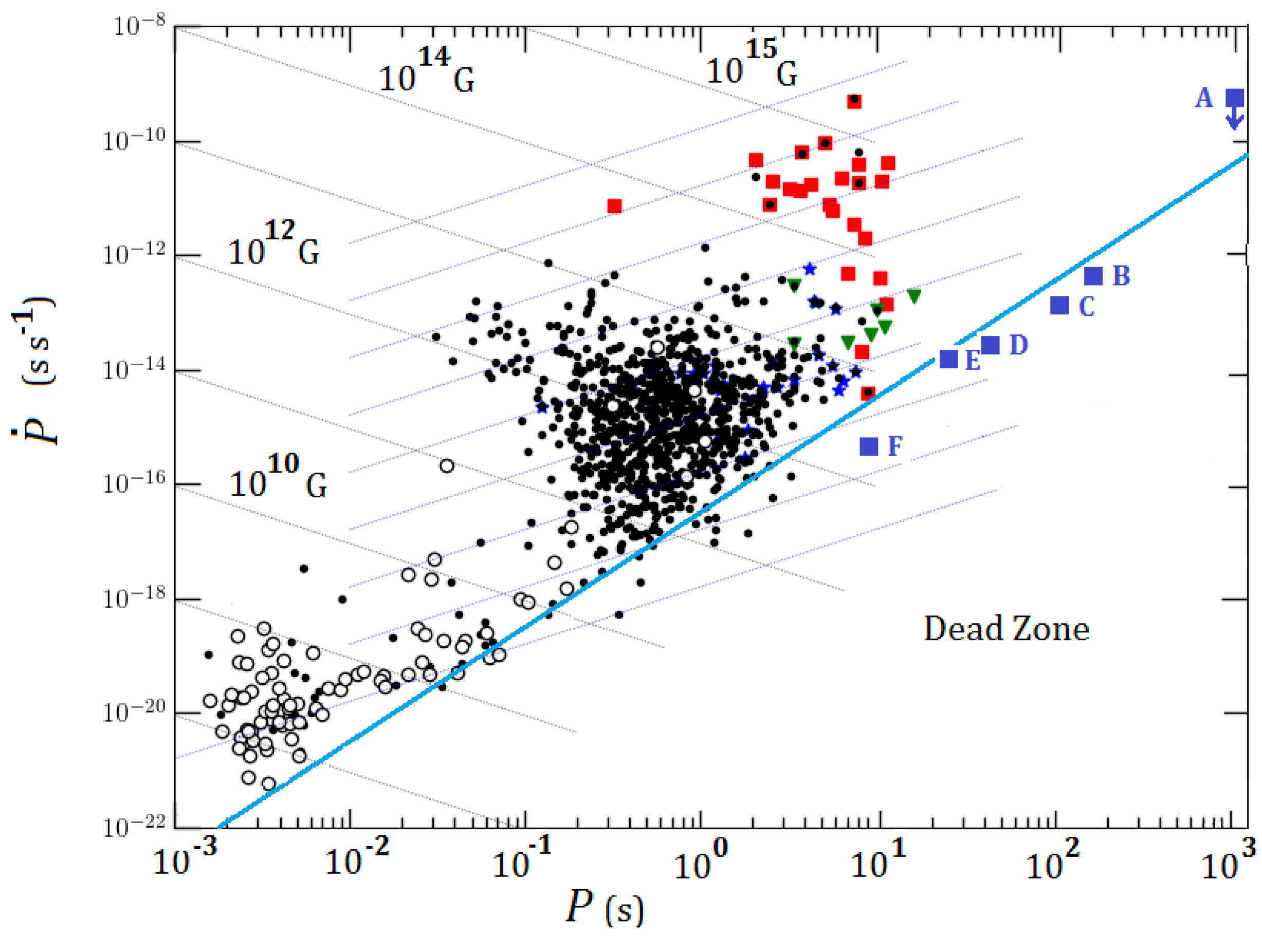
2.1. Neutron Star Demographics
- Do magnetic fields decay?
- Which is the relationship between all these subpopulations?
- Are the new objects old magnetars?
2.2. Neutron Star Mass Distribution
2.3. Neutron Star Radii
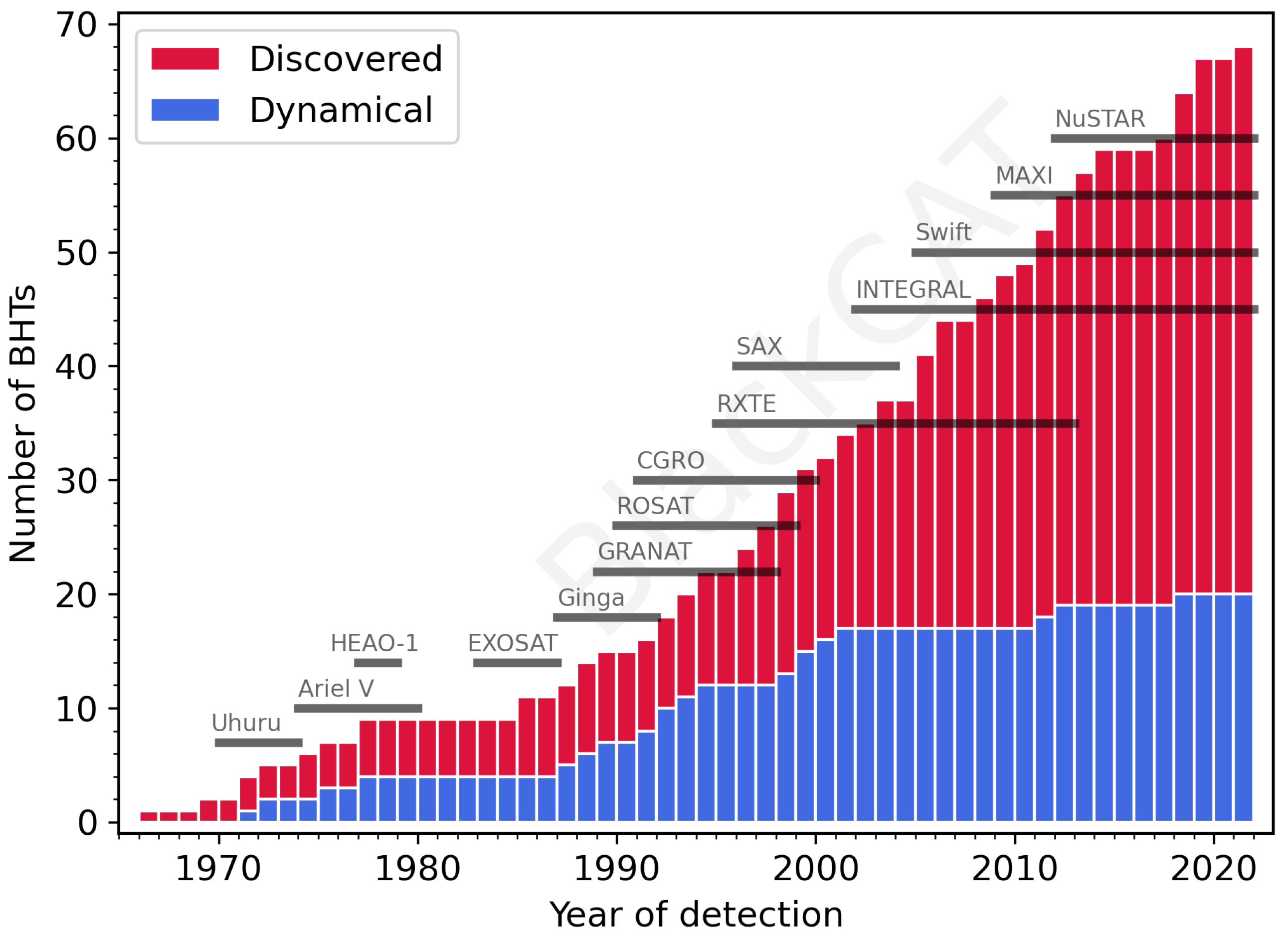
3. Black Holes
3.1. Treatment of Uncertainties
3.2. Nature of Observations
3.3. Mass Computation from Orbital Parameters
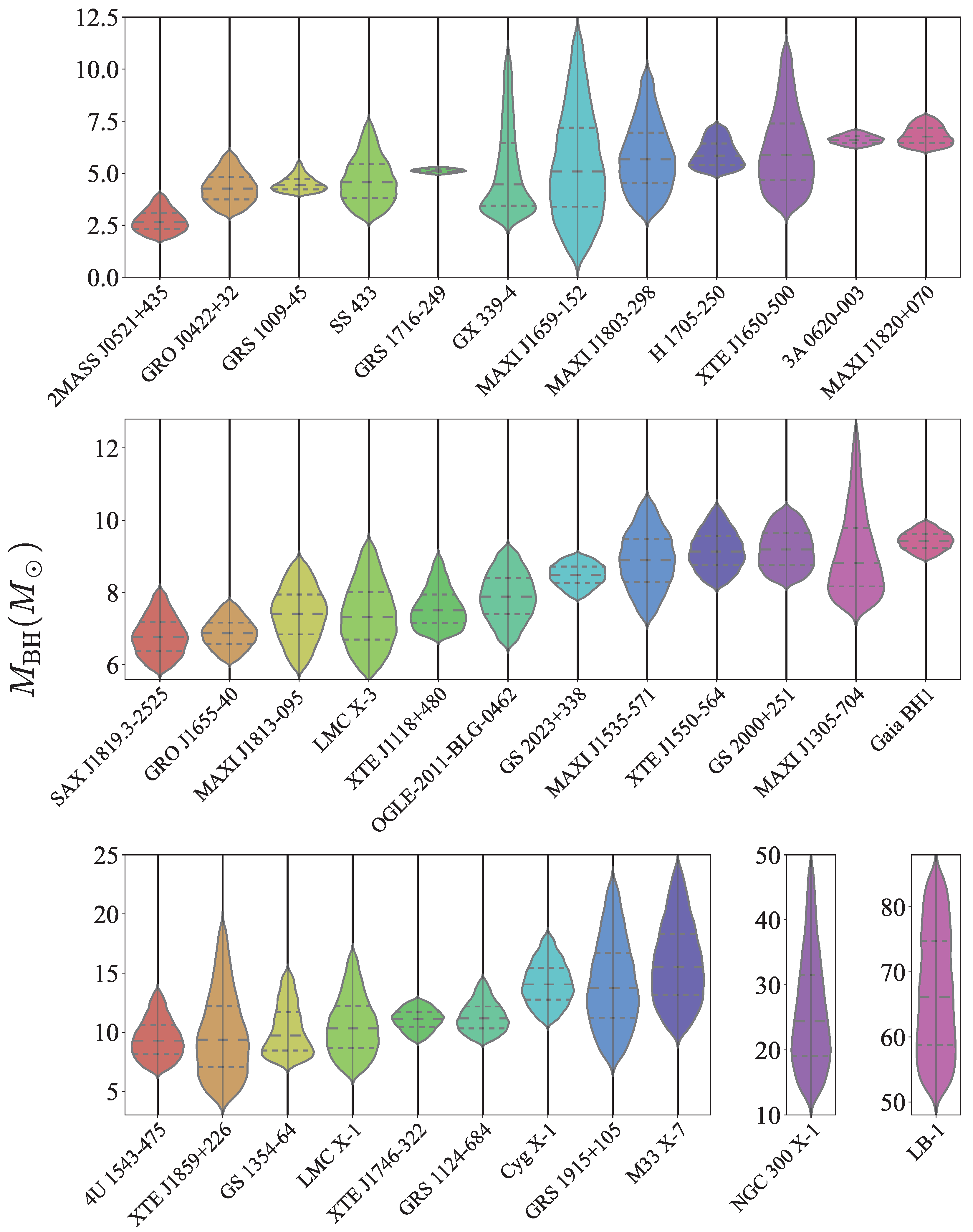
3.4. Collected Systems
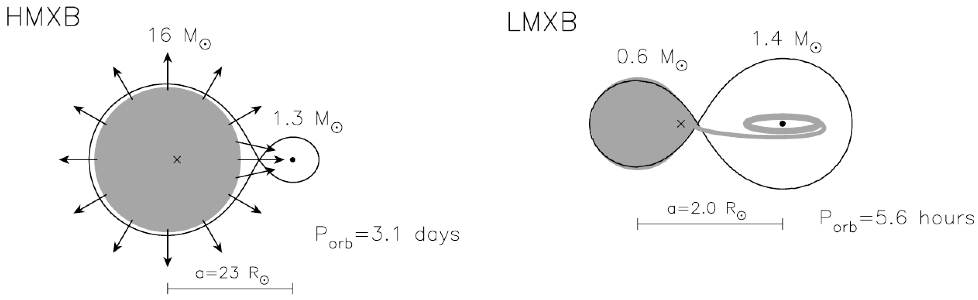
3.4.1. LMXBs
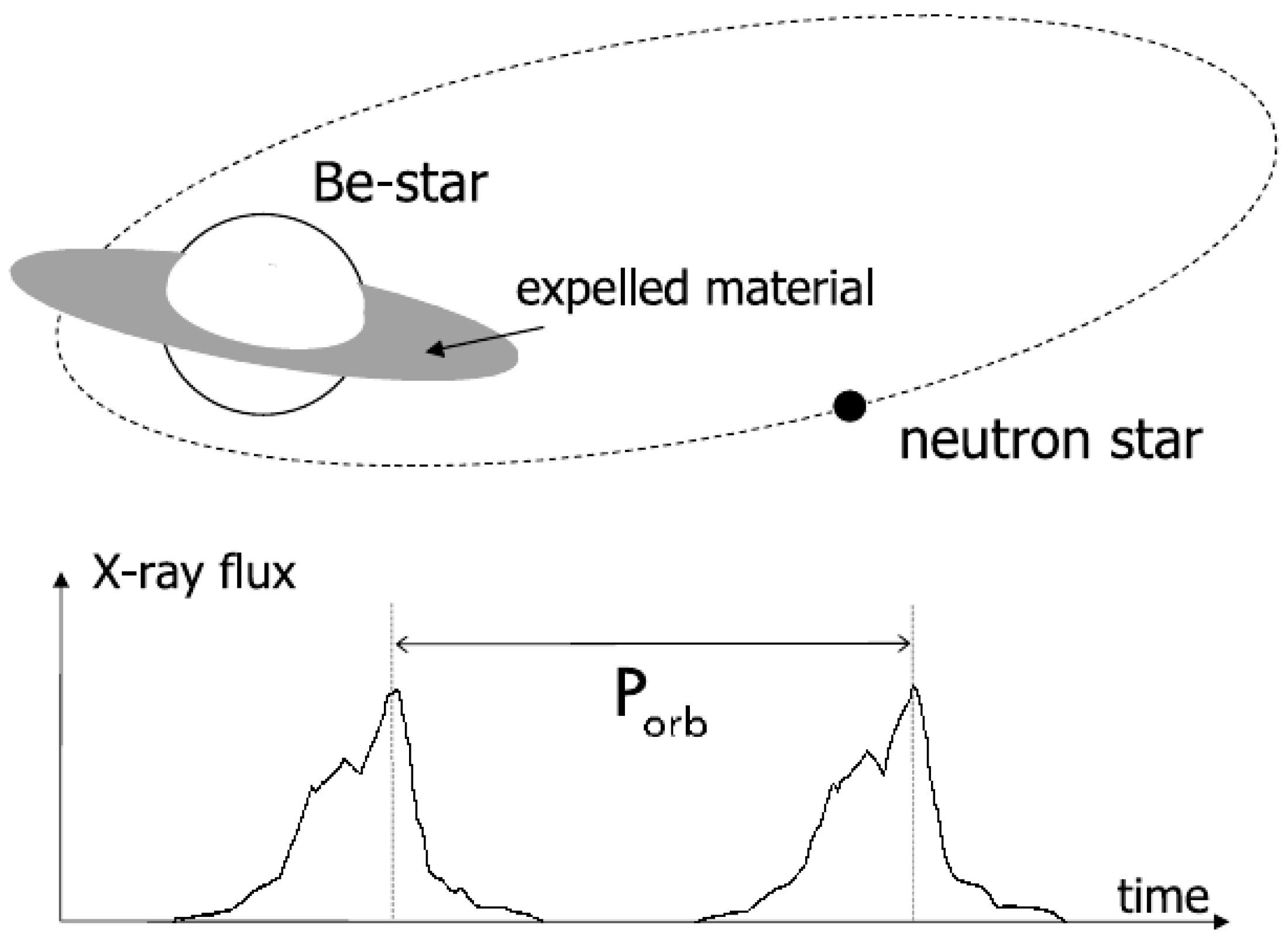
3.4.2. HMXBs
3.4.3. Other Sources

| Name | i | q | References | ||||
|---|---|---|---|---|---|---|---|
| day | km s | deg | |||||
| 4U 1543-475 | [128] | ||||||
| GRS 1915+105 | [129] | ||||||
| GS 1354-64 | [25,130] | ||||||
| GRS 1124-684 | [132,133] | ||||||
| XTE J1118+480 | [134] | ||||||
| 3A 0620-003 | [134] | ||||||
| GS 2000+251 | [144] | ||||||
| MAXI J1659-152 | [146] | ||||||
| MAXI J1305-704 | [147] | ||||||
| GS 2023+338 | [148,149] | ||||||
| XTE J1650-500 | [150] | ||||||
| GRO J0422+32 | [99,151] | ||||||
| H 1705-250 | [152,153] | ||||||
| GRO J1655-40 | [154,155] | ||||||
| XTE J1859+226 | [123,158] | ||||||
| MAXI J1803-298 | [147] | ||||||
| MAXI J1820+070 | [161,162] | ||||||
| XTE J1550-564 | [164] | ||||||
| GX 339-4 | [166] | ||||||
| GRS 1009-45 | [168] | ||||||
| LMC X-3 | [170] | ||||||
| SAX J1819.3-2525 | [171,172] | ||||||
| GRS 1716-249 | - | - | - | - | [174] | ||
| MAXI J1813-095 | - | - | - | - | [175] | ||
| MAXI J1535-571 | - | - | - | - | - | [176] | |
| XTE J1746-322 | - | - | - | - | - | [177] | |
| Cyg X-1 | [124,179] | ||||||
| LMC X-1 | [125] | ||||||
| M33 X-7 | [126,182] | ||||||
| NGC 300 X-1 | [183,184] | ||||||
| SS 433 | [127,185] | ||||||
| LB-1 cp. | [100] | ||||||
| 2MASS J0521+435 cp. | [101] | ||||||
| Gaia BH1 | [102] | ||||||
| OGLE-2011-BLG-0462 | - | - | - | - | - | [187] |
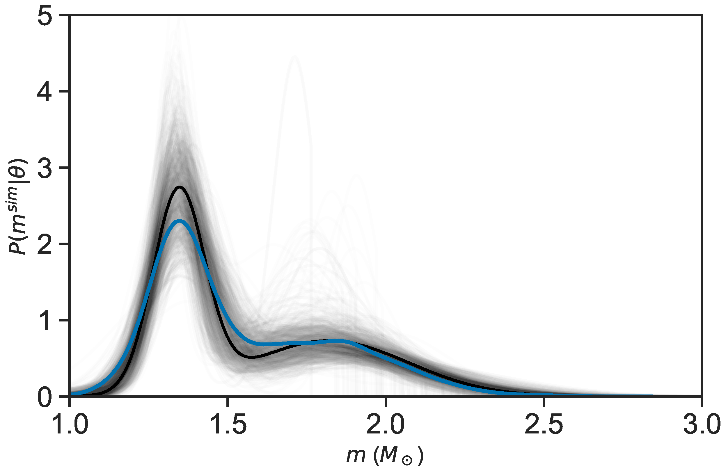
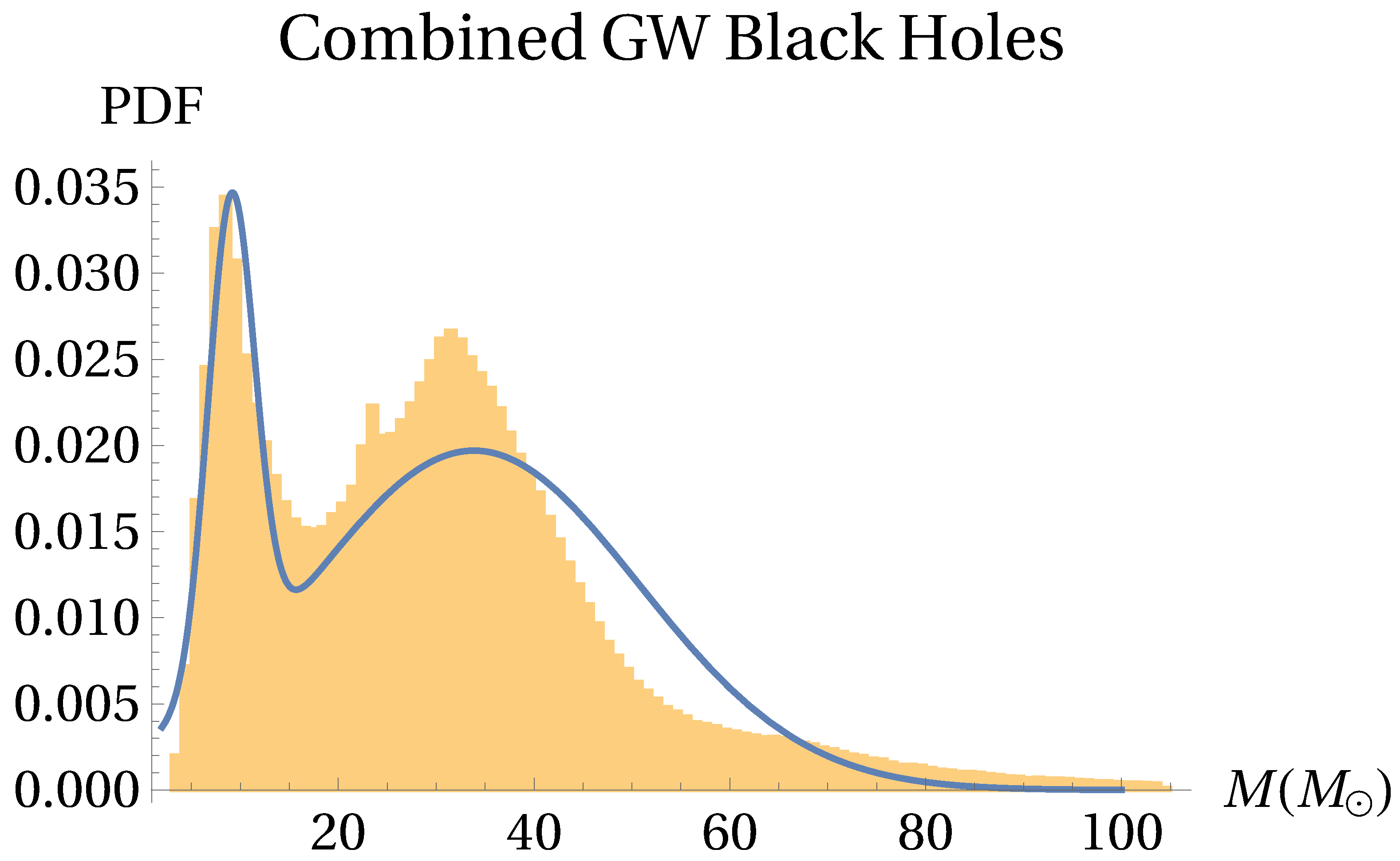
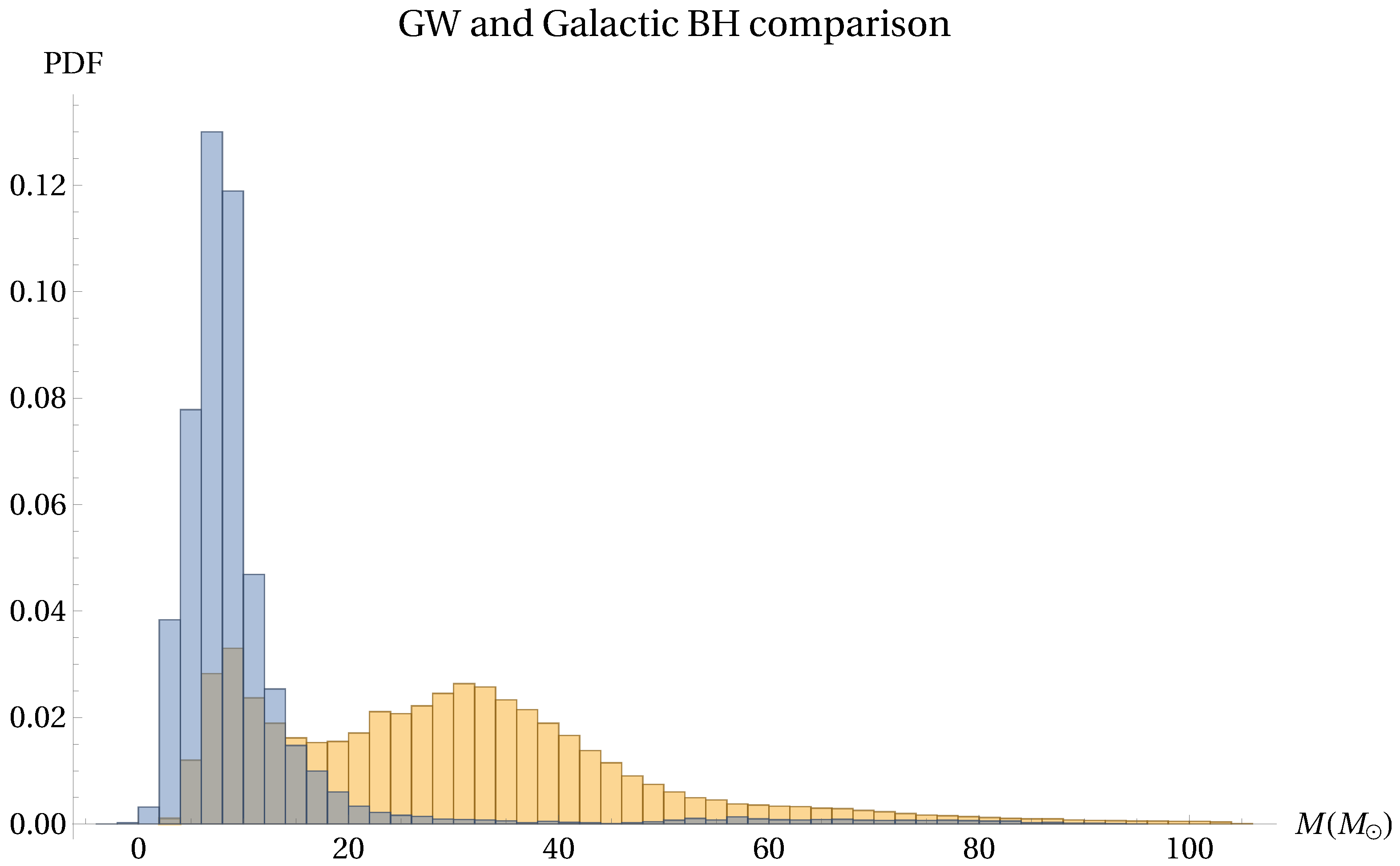
3.5. The Full Mass Distribution
3.6. The Lower Mass Gap
4. Conclusions
Author Contributions
Funding
Data Availability Statement
Acknowledgments
Conflicts of Interest
References
- Walter, F.M.; Wolk, S.J.; Neuhäuser, R. Discovery of a nearby isolated neutron star. Nature 1996, 379, 233–235. [Google Scholar] [CrossRef]
- Zampieri, L.; Campana, S.; Turolla, R.; Chieregato, M.; Falomo, R.; Fugazza, D.; Moretti, A.; Treves, A. 1RXS J214303.7+065419/RBS 1774: A new Isolated Neutron Star candidate. Astron. Astrophys. 2001, 378, L5–L9. [Google Scholar] [CrossRef]
- Turolla, R. Isolated Neutron Stars: The Challenge of Simplicity. In Proceedings of the Astrophysics and Space Science Library; Becker, W., Ed.; Springer: Berlin, Germany, 2009; Volume 357, p. 141. [Google Scholar] [CrossRef]
- Ertan, Ü.; Çalışkan, Ş.; Benli, O.; Alpar, M.A. Long-term evolution of dim isolated neutron stars. Mon. Not. R. Astron. Soc. 2014, 444, 1559–1565. [Google Scholar] [CrossRef] [Green Version]
- Esposito, P.; Rea, N.; Israel, G.L. Magnetars: A Short Review and Some Sparse Considerations. In Proceedings of the Astrophysics and Space Science Library; Belloni, T.M., Méndez, M., Zhang, C., Eds.; Astrophysics and Space Science Library: New York, NY, USA, 2021; Volume 461, pp. 97–142. [Google Scholar] [CrossRef]
- De Luca, A. Central compact objects in supernova remnants. In Proceedings of the Journal of Physics Conference Series; IOP Publishing: Bristol, UK, 2017; Volume 932, p. 012006. [Google Scholar] [CrossRef]
- Mayer, M.G.F.; Becker, W. A kinematic study of central compact objects and their host supernova remnants. Astron. Astrophys. 2021, 651, A40. [Google Scholar] [CrossRef]
- Ho, W.C.G. Central compact objects and their magnetic fields. In Proceedings of the Neutron Stars and Pulsars: Challenges and Opportunities after 80 Years; van Leeuwen, J., Ed.; Cambridge University Press: Cambridge, UK, 2013; Volume 291, pp. 101–106. [Google Scholar] [CrossRef] [Green Version]
- Ho, W.C.G.; Zhao, Y.; Heinke, C.O.; Kaplan, D.L.; Shternin, P.S.; Wijngaarden, M.J.P. X-ray bounds on cooling, composition, and magnetic field of the Cassiopeia A neutron star and young central compact objects. Mon. Not. R. Astron. Soc. 2021, 506, 5015–5029. [Google Scholar] [CrossRef]
- Abhishek; Malusare, N.; Tanushree, N.; Hegde, G.; Konar, S. Radio pulsar sub-populations (II): The mysterious RRATs. J. Astrophys. Astron. 2022, 43, 75. [Google Scholar] [CrossRef]
- Keane, E.F.; McLaughlin, M.A. Rotating radio transients. Bull. Astron. Soc. India 2011, 39, 333–352. [Google Scholar]
- Hurley-Walker, N.; Zhang, X.; Bahramian, A.; McSweeney, S.J.; O’Doherty, T.N.; Hancock, P.J.; Morgan, J.S.; Anderson, G.E.; Heald, G.H.; Galvin, T.J. A radio transient with unusually slow periodic emission. Nature 2022, 601, 526–530. [Google Scholar] [CrossRef]
- Corral-Santana, J.M.; Casares, J.; Muñoz-Darias, T.; Bauer, F.E.; Martínez-Pais, I.G.; Russell, D.M. BlackCAT: A catalogue of stellar-mass black holes in X-ray transients. Astron. Astrophys. 2016, 587, A61. [Google Scholar] [CrossRef] [Green Version]
- Tetarenko, B.E.; Sivakoff, G.R.; Heinke, C.O.; Gladstone, J.C. WATCHDOG: A Comprehensive All-sky Database of Galactic Black Hole X-ray Binaries. Astrophys. J. Suppl. Ser. 2016, 222, 15. [Google Scholar] [CrossRef] [Green Version]
- Ingram, A.R.; Motta, S.E. A review of quasi-periodic oscillations from black hole X-ray binaries: Observation and theory. New Astron. Rev. 2019, 85, 101524. [Google Scholar] [CrossRef] [Green Version]
- Lam, C.Y.; Lu, J.R.; Udalski, A.; Bond, I.; Bennett, D.P.; Skowron, J.; Mróz, P.; Poleski, R.; Sumi, T.; Szymański, M.K.; et al. An Isolated Mass-gap Black Hole or Neutron Star Detected with Astrometric Microlensing. Astrophys. J. 2022, 933, L23. [Google Scholar] [CrossRef]
- Sahu, K.C.; Anderson, J.; Casertano, S.; Bond, H.E.; Udalski, A.; Dominik, M.; Calamida, A.; Bellini, A.; Brown, T.M.; Rejkuba, M.; et al. An Isolated Stellar-mass Black Hole Detected through Astrometric Microlensing. Astrophys. J. 2022, 933, 83. [Google Scholar] [CrossRef]
- Burrows, A.; Vartanyan, D. Core-collapse supernova explosion theory. Nature 2021, 589, 29–39. [Google Scholar] [CrossRef] [PubMed]
- Ertl, T.; Woosley, S.E.; Sukhbold, T.; Janka, H.T. The Explosion of Helium Stars Evolved with Mass Loss. Astrophys. J. 2020, 890, 51. [Google Scholar] [CrossRef] [Green Version]
- Tauris, T.M.; Sanyal, D.; Yoon, S.C.; Langer, N. Evolution towards and beyond accretion-induced collapse of massive white dwarfs and formation of millisecond pulsars. Astron. Astrophys. 2013, 558, A39. [Google Scholar] [CrossRef] [Green Version]
- Wang, B.; Liu, D. The formation of neutron star systems through accretion-induced collapse in white-dwarf binaries. Res. Astron. Astrophys. 2020, 20, 135. [Google Scholar] [CrossRef]
- Wang, B.; Liu, D.; Chen, H. Formation of millisecond pulsars with long orbital periods by accretion-induced collapse of white dwarfs. Mon. Not. R. Astron. Soc. 2022, 510, 6011–6021. [Google Scholar] [CrossRef]
- Bailyn, C.D.; Jain, R.K.; Coppi, P.; Orosz, J.A. The Mass Distribution of Stellar Black Holes. Astrophys. J. 1998, 499, 367–374. [Google Scholar] [CrossRef] [Green Version]
- Özel, F.; Psaltis, D.; Narayan, R.; McClintock, J.E. The black hole mass distribution in the galaxy. Astrophys. J. 2010, 725, 1918. [Google Scholar] [CrossRef] [Green Version]
- Farr, W.M.; Sravan, N.; Cantrell, A.; Kreidberg, L.; Bailyn, C.D.; Mandel, I.; Kalogera, V. The mass distribution of stellar-mass black holes. Astrophys. J. 2011, 741, 103. [Google Scholar] [CrossRef] [Green Version]
- Fryer, C.L.; Belczynski, K.; Wiktorowicz, G.; Dominik, M.; Kalogera, V.; Holz, D.E. Compact Remnant Mass Function: Dependence on the Explosion Mechanism and Metallicity. Astrophys. J. 2012, 749, 91. [Google Scholar] [CrossRef]
- Belczynski, K.; Wiktorowicz, G.; Fryer, C.L.; Holz, D.E.; Kalogera, V. Missing Black Holes Unveil the Supernova Explosion Mechanism. Astrophys. J. 2012, 757, 91. [Google Scholar] [CrossRef] [Green Version]
- Farah, A.; Fishbach, M.; Essick, R.; Holz, D.E.; Galaudage, S. Bridging the Gap: Categorizing Gravitational-wave Events at the Transition between Neutron Stars and Black Holes. Astrophys. J. 2022, 931, 108. [Google Scholar] [CrossRef]
- de Sá, L.M.; Bernardo, A.; Bachega, R.R.A.; Horvath, J.E.; Rocha, L.S.; Moraes, P.H.R.S. Quantifying the Evidence Against a Mass Gap between Black Holes and Neutron Stars. Astrophys. J. 2022, 941, 130. [Google Scholar] [CrossRef]
- Ye, C.; Fishbach, M. Inferring the Neutron Star Maximum Mass and Lower Mass Gap in Neutron Star–Black Hole Systems with Spin. Astrophys. J. 2022, 937, 73. [Google Scholar] [CrossRef]
- Landau, L. On the Theory of Stars. Phys. Z. Sowjetunion 1932, 1, 285–288. [Google Scholar]
- Baade, W.; Zwicky, F. On Super-Novae. Proc. Natl. Acad. Sci. USA 1934, 20, 254–259. [Google Scholar] [CrossRef]
- Hewish, A.; Bell, S.J.; Pilkington, J.D.H.; Scott, P.F.; Collins, R.A. Observation of a Rapidly Pulsating Radio Source. Nature 1968, 217, 709–713. [Google Scholar] [CrossRef]
- Pacini, F. Rotating Neutron Stars, Pulsars and Supernova Remnants. Nature 1968, 219, 145–146. [Google Scholar] [CrossRef] [Green Version]
- Gold, T. Rotating Neutron Stars as the Origin of the Pulsating Radio Sources. Nature 1968, 218, 731–732. [Google Scholar] [CrossRef]
- Horvath, J.; Rocha, L.; Bernardo, A.C.; de Avellar, M.; Valentim, R. Birth events, masses and the maximum mass of Compact Stars. In Astrophysics in the XXI Century with Compact Stars; Vasconcellos, C.Z., Weber, F., Eds.; World Scientific Publishing: Singapore, 2022; pp. 1–51. [Google Scholar]
- Bisnovatyi-Kogan, G.S. The Neutron Star Population in the Galaxy. In Proceedings of IAU Symposium #149; Barbuy, B., Renzini, A., Eds.; Spinger: Dordrecht, The Netherlands, 1992; Volume 149, p. 379. [Google Scholar]
- Lyne, A.G.; Manchester, R.N.; Taylor, J.H. The galactic population of pulsars. Mon. Not. R. Astron. Soc. 1985, 213, 613–639. [Google Scholar] [CrossRef] [Green Version]
- Dirson, L.; Pétri, J.; Mitra, D. The Galactic population of canonical pulsars. Astron. Astrophys. 2022, 667, A82. [Google Scholar] [CrossRef]
- Kaspi, V.M. Grand unification of neutron stars. Proc. Natl. Acad. Sci. USA 2010, 107, 7147–7152. [Google Scholar] [CrossRef] [Green Version]
- Rutledge, R.E.; Fox, D.B.; Shevchuk, A.H. Discovery of an Isolated Compact Object at High Galactic Latitude. Astrophys. J. 2008, 672, 1137–1143. [Google Scholar] [CrossRef] [Green Version]
- Potekhin, A.Y.; De Luca, A.; Pons, J.A. Neutron Stars—Thermal Emitters. Space Sci. Rev. 2015, 191, 171–206. [Google Scholar] [CrossRef] [Green Version]
- Buckley, D.A.H.; Meintjes, P.J.; Potter, S.B.; Marsh, T.R.; Gänsicke, B.T. Polarimetric evidence of a white dwarf pulsar in the binary system AR Scorpii. Nat. Astron. 2017, 1, 29. [Google Scholar] [CrossRef] [Green Version]
- Caleb, M.; Heywood, I.; Rajwade, K.; Malenta, M.; Stappers, B.W.; Barr, E.; Chen, W.; Morello, V.; Sanidas, S.; van den Eijnden, J.; et al. Discovery of a radio-emitting neutron star with an ultra-long spin period of 76 s. Nat. Astron. 2022, 6, 828–836. [Google Scholar] [CrossRef]
- Agar, C.H.; Weltevrede, P.; Bondonneau, L.; Grießmeier, J.M.; Hessels, J.W.T.; Huang, W.J.; Karastergiou, A.; Keith, M.J.; Kondratiev, V.I.; Künsemöller, J.; et al. A broad-band radio study of PSR J0250+5854: The slowest spinning radio pulsar known. Mon. Not. R. Astron. Soc. 2021, 508, 1102–1114. [Google Scholar] [CrossRef]
- Morello, V.; Keane, E.F.; Enoto, T.; Guillot, S.; Ho, W.C.G.; Jameson, A.; Kramer, M.; Stappers, B.W.; Bailes, M.; Barr, E.D.; et al. The SUrvey for Pulsars and Extragalactic Radio Bursts – IV. Discovery and polarimetry of a 12.1-s radio pulsar. Mon. Not. R. Astron. Soc. 2020, 493, 1165–1177. [Google Scholar] [CrossRef] [Green Version]
- Young, M.D.; Manchester, R.N.; Johnston, S. A radio pulsar with an 8.5-second period that challenges emission models. Nature 1999, 400, 848–849. [Google Scholar] [CrossRef]
- Turolla, R.; Esposito, P. Low-magnetic-field magnetars. Int. J. Mod. Phys. D 2013, 22, 1330024. [Google Scholar] [CrossRef]
- Viganò, D.; Rea, N.; Pons, J.A.; Perna, R.; Aguilera, D.N.; Miralles, J.A. Unifying the observational diversity of isolated neutron stars via magneto-thermal evolution models. Mon. Not. R. Astron. Soc. 2013, 434, 123–141. [Google Scholar] [CrossRef]
- Igoshev, A.P.; Popov, S.B.; Hollerbach, R. Evolution of Neutron Star Magnetic Fields. Universe 2021, 7, 351. [Google Scholar] [CrossRef]
- Benvenuto, O.G.; De Vito, M.A.; Horvath, J.E. Understanding the Evolution of Close Binary Systems with Radio Pulsars. Astrophys. J. 2014, 786, L7. [Google Scholar] [CrossRef] [Green Version]
- Mendes, C.; de Avellar, M.G.B.; Horvath, J.E.; Souza, R.A.d.; Benvenuto, O.G.; De Vito, M.A. Magnetic field decay in black widow pulsars. Mon. Not. R. Astron. Soc. 2018, 475, 2178–2184. [Google Scholar] [CrossRef] [Green Version]
- Igoshev, A.P.; Popov, S.B. Braking indices of young radio pulsars: Theoretical perspective. Mon. Not. R. Astron. Soc. 2020, 499, 2826–2835. [Google Scholar] [CrossRef]
- Allen, M.P.; Horvath, J.E. Glitches, torque evolution and the dynamics of young pulsars. Mon. Not. R. Astron. Soc. 1997, 287, 615–621. [Google Scholar] [CrossRef]
- Yoneyama, T.; Hayashida, K.; Nakajima, H.; Matsumoto, H. Unification of strongly magnetized neutron stars with regard to X-ray emission from hot spots. Astron. Nachrichten 2019, 340, 221–225. Available online: https://onlinelibrary.wiley.com/doi/pdf/10.1002/asna.201913593 (accessed on 21 December 2022). [CrossRef] [Green Version]
- Hurley, K. Soft gamma repeaters. Mem. Soc. Astron. Ital. 2010, 81, 432. [Google Scholar] [CrossRef]
- Kaspi, V.M. Recent progress on anomalous X-ray pulsars. Astrophys. Space Sci. 2007, 308, 1–11. [Google Scholar] [CrossRef] [Green Version]
- Keane, E.F. Classifying RRATs and FRBs. Mon. Not. R. Astron. Soc. 2016, 459, 1360–1362. [Google Scholar] [CrossRef] [Green Version]
- Kaspi, V.M.; Kramer, M. Radio Pulsars: The Neutron Star Population & Fundamental Physics. arXiv 2016, arXiv:1602.07738. [Google Scholar]
- Beniamini, P.; Wadiasingh, Z.; Hare, J.; Rajwade, K.; Younes, G.; van der Horst, A.J. Evidence for an abundant old population of Galactic Ultra long period magnetars and implications for fast radio bursts. arXiv 2022, arXiv:2210.09323. [Google Scholar] [CrossRef]
- Rocha, L.S.; Bachega, R.R.A.; Horvath, J.E.; Moraes, P.H.R.S. The maximum mass of neutron stars may be higher than expected: An inference from binary systems. arXiv 2021, arXiv:2107.08822. [Google Scholar] [CrossRef]
- Postnov, K.A.; Prokhorov, M.E. The Relation between the Observed Mass Distribution for Compact Stars and the Mechanism for Supernova Explosions. Astron. Rep. 2001, 45, 899–907. [Google Scholar] [CrossRef]
- Valentim, R.; Rangel, E.; Horvath, J. On the mass distribution of neutron stars. Mon. Not. R. Astron. Soc. 2011, 414, 1427–1431. [Google Scholar] [CrossRef]
- Özel, F.; Freire, P. Masses, radii, and the equation of state of neutron stars. Annu. Rev. Astron. Astrophys. 2016, 54, 401–440. [Google Scholar] [CrossRef] [Green Version]
- Kiziltan, B.; Kottas, A.; De Yoreo, M.; Thorsett, S.E. The neutron star mass distribution. Astrophys. J. 2013, 778, 66. [Google Scholar] [CrossRef]
- Zhang, W.; Strohmayer, T.; Swank, J. Neutron star masses and radii as inferred from kilohertz quasi-periodic oscillations. Astrophys. J. 1997, 482, L167. [Google Scholar] [CrossRef] [Green Version]
- Alsing, J.; Silva, H.O.; Berti, E. Evidence for a maximum mass cut-off in the neutron star mass distribution and constraints on the equation of state. Mon. Not. R. Astron. Soc. 2018, 478, 1377–1391. [Google Scholar] [CrossRef] [Green Version]
- Rhoades, C.E.; Ruffini, R. Maximum Mass of a Neutron Star. Phys. Rev. Lett. 1974, 32, 324–327. [Google Scholar] [CrossRef] [Green Version]
- Margalit, B.; Metzger, B.D. Constraining the Maximum Mass of Neutron Stars from Multi-messenger Observations of GW170817. Astrophys. J. Lett. 2017, 850, L19. [Google Scholar] [CrossRef]
- Rezzolla, L.; Most, E.R.; Weih, L.R. Using Gravitational-wave Observations and Quasi-universal Relations to Constrain the Maximum Mass of Neutron Stars. Astrophys. J. Lett. 2018, 852, L25. [Google Scholar] [CrossRef]
- Ruiz, M.; Shapiro, S.L.; Tsokaros, A. GW170817, general relativistic magnetohydrodynamic simulations, and the neutron star maximum mass. Phys. Rev. D 2018, 97, 021501. [Google Scholar] [CrossRef] [Green Version]
- Shibata, M.; Zhou, E.; Kiuchi, K.; Fujibayashi, S. Constraint on the maximum mass of neutron stars using GW170817 event. Phys. Rev. D 2019, 100, 023015. [Google Scholar] [CrossRef] [Green Version]
- Ai, S.; Gao, H.; Zhang, B. What Constraints on the Neutron Star Maximum Mass Can One Pose from GW170817 Observations? Astrophys. J. 2020, 893, 146. [Google Scholar] [CrossRef]
- Romani, R.; Kandel, D.; Filippenko, A.; Brink, T.; Zheng, W. PSR J0952-0607: The Fastest and Heaviest Known Galactic Neutron Star. Astrophys. J. Lett. 2022, 934, L17. [Google Scholar] [CrossRef]
- Ecker, C.; Rezzolla, L. Impact of large-mass constraints on the properties of neutron stars. arXiv 2022, arXiv:2209.08101. [Google Scholar] [CrossRef]
- Abbott, R.; Abbott, T.D.; Acernese, F.; Ackley, K.; Adams, C.; Adhikari, N.; Adhikari, R.X.; Adya, V.B.; Affeldt, C.; Agarwal, D.; et al. GWTC-3: Compact Binary Coalescences Observed by LIGO and Virgo During the Second Part of the Third Observing Run. arXiv 2021, arXiv:2111.03606. [Google Scholar] [CrossRef]
- Doroshenko, V.; Suleimanov, V.; Pühlhofer, G.; Santangelo, A. A strangely light neutron star within a supernova remnant. Nat. Astron. 2022, 6, 1444–1451. [Google Scholar] [CrossRef]
- Di Clemente, F.; Drago, A.; Pagliara, G. Is the compact object associated with HESS J1731-347 a strange quark star? arXiv 2022, arXiv:2211.07485. [Google Scholar]
- Weber, F. Strange quark matter and compact stars. Prog. Part. Nucl. Phys. 2005, 54, 193–288. [Google Scholar] [CrossRef] [Green Version]
- Martinez, J.G.; Stovall, K.; Freire, P.C.C.; Deneva, J.S.; Jenet, F.A.; McLaughlin, M.A.; Bagchi, M.; Bates, S.D.; Ridolfi, A. Pulsar J0453+1559: A double neutron star system with a large mass asymmetry. Astrophys. J. 2015, 812, 143. [Google Scholar] [CrossRef] [Green Version]
- Fonseca, E.; Pennucci, T.T.; Ellis, J.A.; Stairs, I.H.; Nice, D.J.; Ransom, S.M.; Demorest, P.B.; Arzoumanian, Z.; Crowter, K.; Dolch, T.; et al. The NANOGrav Nine-year Data Set: Mass and Geometric Measurements of Binary Millisecond Pulsars. Astrophys. J. 2016, 832, 167. [Google Scholar] [CrossRef]
- Lattimer, J.M. Neutron Star Mass and Radius Measurements. Universe 2019, 5, 159. [Google Scholar] [CrossRef] [Green Version]
- Riley, T.E.; Watts, A.L.; Ray, P.S.; Bogdanov, S.; Guillot, S.; Morsink, S.M.; Bilous, A.V.; Arzoumanian, Z.; Choudhury, D.; Deneva, J.S.; et al. A NICER View of the Massive Pulsar PSR J0740+6620 Informed by Radio Timing and XMM-Newton Spectroscopy. Astrophys. J. 2021, 918, L27. [Google Scholar] [CrossRef]
- Riley, T.E.; Watts, A.L.; Bogdanov, S.; Ray, P.S.; Ludlam, R.M.; Guillot, S.; Arzoumanian, Z.; Baker, C.L.; Bilous, A.V.; Chakrabarty, D.; et al. A NICER View of PSR J0030+0451: Millisecond Pulsar Parameter Estimation. Astrophys. J. 2019, 887, L21. [Google Scholar] [CrossRef] [Green Version]
- Horvath, J.; Moraes, P.H.R.S. Modeling a 2.5Mo compact star with quark matter. Int. Jour. Mod. Phys. D 2021, 30, 2150016. [Google Scholar] [CrossRef]
- Einstein, A. Die Feldgleichungen der Gravitation; Sitzungsberichte der Preussischen Akademie der Wissenschaften zu Berlin: Berlin, Germany, 1915; pp. 844–847. [Google Scholar]
- Schwarzschild, K. On the Gravitational Field of a Mass Point According to Einstein’s Theory. Abh. Konigl. Preuss. Akad. 1916, 189–196. [Google Scholar]
- Kerr, R.P. Gravitational Field of a Spinning Mass as an Example of Algebraically Special Metrics. Phys. Rev. Lett. 1963, 11, 237–238. [Google Scholar] [CrossRef]
- Newman, E.T.; Couch, E.; Chinnapared, K.; Exton, A.; Prakash, A.; Torrence, R. Metric of a Rotating, Charged Mass. J. Math. Phys. 1965, 6, 918–919. [Google Scholar] [CrossRef]
- ’t Hooft, G. The Black hole horizon as a quantum surface. Phys. Scr. 1991, 36, 247–252. [Google Scholar] [CrossRef]
- Hawking, S.W. The information paradox for black holes. arXiv 2015, arXiv:1509.01147. [Google Scholar]
- Susskind, L. The paradox of quantum black holes. Nat. Phys. 2006, 2, 665–677. [Google Scholar] [CrossRef]
- Oppenheimer, J.R.; Volkoff, G.M. On Massive Neutron Cores. Phys. Rev. 1939, 55, 374–381. [Google Scholar] [CrossRef]
- Tolman, R.C. Static Solutions of Einstein’s Field Equations for Spheres of Fluid. Phys. Rev. 1939, 55, 364–373. [Google Scholar] [CrossRef] [Green Version]
- Zel’dovich, Y.B. The fate of a star, and the liberation of gravitation energy in accretion. Dokl. Akad. Nauk SSSR 1964, 155, 67–69. [Google Scholar]
- Salpeter, E.E. Accretion of Interstellar Matter by Massive Objects. Astrophys. J. 1964, 140, 796–800. [Google Scholar] [CrossRef]
- Bolton, C.T. Identification of Cygnus X-1 with HDE 226868. Nature 1972, 235, 271–273. [Google Scholar] [CrossRef]
- Webster, B.L.; Murdin, P. Cygnus X-1-a Spectroscopic Binary with a Heavy Companion ? Nature 1972, 235, 37–38. [Google Scholar] [CrossRef]
- Gelino, D.M.; Harrison, T.E. GRO J0422+32: The Lowest Mass Black Hole? Astrophys. J. 2003, 599, 1254–1259. [Google Scholar] [CrossRef] [Green Version]
- Liu, J.; Zhang, H.; Howard, A.W.; Bai, Z.; Lu, Y.; Soria, R.; Justham, S.; Li, X.; Zheng, Z.; Wang, T.; et al. A wide star–black-hole binary system from radial-velocity measurements. Nature 2019, 575, 618–621. [Google Scholar] [CrossRef]
- Thompson, T.A.; Kochanek, C.S.; Stanek, K.Z.; Badenes, C.; Post, R.S.; Jayasinghe, T.; Latham, D.W.; Bieryla, A.; Esquerdo, G.A.; Berlind, P.; et al. A noninteracting low-mass black hole-giant star binary system. Science 2019, 366, 637–640. [Google Scholar] [CrossRef] [Green Version]
- El-Badry, K.; Rix, H.W.; Quataert, E.; Howard, A.W.; Isaacson, H.; Fuller, J.; Hawkins, K.; Breivik, K.; Wong, K.W.K.; Rodriguez, A.C.; et al. A Sun-like star orbiting a black hole. Mon. Not. R. Astron. Soc. 2022, 518, 1057–1085. [Google Scholar] [CrossRef]
- King, A.R. Accretion in compact binaries. In Compact Stellar X-ray Sources; Cambridge University Press: Cambridge, UK, 2006; Volume 39, pp. 507–546. [Google Scholar]
- Shakura, N.I.; Sunyaev, R.A. Black holes in binary systems. Observational appearance. Astron. Atrophys. 1973, 24, 337–355. [Google Scholar]
- Shapiro, S.L.; Lightman, A.P.; Eardley, D.M. A two-temperature accretion disk model for Cygnus X-1: Structure and spectrum. Astrophys. J. 1976, 204, 187–199. [Google Scholar] [CrossRef]
- Frank, J.; King, A.; Raine, D.J. Accretion Power in Astrophysics, 3rd ed.; Cambridge University Press: Cambridge, UK, 2002. [Google Scholar]
- Liao, Z.; Liu, J.; Zheng, X.; Gou, L. Spectral evidence of an accretion disc in wind-fed X-ray pulsar Vela X-1 during an unusual spin-up period. Mon. Not. R. Astron. Soc. 2020, 492, 5922–5929. [Google Scholar] [CrossRef] [Green Version]
- Tauris, T.M.; van den Heuvel, E.P.J. Formation and evolution of compact stellar X-ray sources. In Compact Stellar X-ray Sources; Cambridge University Press: Cambridge, UK, 2006; Volume 39, pp. 623–665. [Google Scholar]
- Hameury, J. A review of the disc instability model for dwarf novae, soft X-ray transients and related objects. Adv. Space Res. 2020, 66, 1004–1024. [Google Scholar] [CrossRef] [Green Version]
- Tremaine, S.; Davis, S.W. Dynamics of warped accretion discs. Mon. Not. R. Astron. Soc. 2014, 441, 1408–1434. Available online: https://academic.oup.com/mnras/article-pdf/441/2/1408/3724550/stu663.pdf (accessed on 21 December 2022). [CrossRef]
- Abarr, Q.; Krawczynski, H. Exploring the Physics of Warped Accretion Disks with the Imaging X-ray Polarimetry Explorer. In Proceedings of the American Astronomical Society Meeting Abstracts #235. Am. Astron. Soc. Meet. Abstr. 2020, 235, 346.02. [Google Scholar]
- Bagnoli, T.; in’t Zand, J.J.M.; D’Angelo, C.R.; Galloway, D.K. A population study of type II bursts in the Rapid Burster. Mon. Not. R. Astron. Soc. 2015, 449, 268–287. [Google Scholar] [CrossRef] [Green Version]
- Reig, P. Be/X-ray binaries. Astrophys. Space Sci. 2011, 332, 1–29. [Google Scholar] [CrossRef] [Green Version]
- Ribó, M.; Munar-Adrover, P.; Paredes, J.M.; Marcote, B.; Iwasawa, K.; Moldón, J.; Casares, J.; Migliari, S.; Paredes-Fortuny, X. The First Simultaneous X-ray/Radio Detection of the First Be/BH System MWC 656. Astrophys. J. Lett. 2017, 835, L33. [Google Scholar] [CrossRef] [Green Version]
- Lutovinov, A.A.; Revnivtsev, M.G.; Tsygankov, S.S.; Krivonos, R.A. Population of persistent high-mass X-ray binaries in the Milky Way. Mon. Not. R. Astron. Soc. 2013, 431, 327–341. [Google Scholar] [CrossRef]
- Sguera, V.; Barlow, E.J.; Bird, A.J.; Clark, D.J.; Dean, A.J.; Hill, A.B.; Moran, L.; Shaw, S.E.; Willis, D.R.; Bazzano, A.; et al. INTEGRAL observations of recurrent fast X-ray transient sources. Astron. Astrophys. 2005, 444, 221–231. [Google Scholar] [CrossRef] [Green Version]
- Negueruela, I.; Smith, D.M.; Reig, P.; Chaty, S.; Torrejón, J.M. Supergiant Fast X-ray Transients: A New Class of High Mass X-ray Binaries Unveiled by INTEGRAL. In Proceedings of the The X-ray Universe 2005; Wilson, A., Ed.; ESA Publications Division: Noordwijk, The Netherlands, 2006; Volume 604, p. 165. [Google Scholar]
- Sidoli, L. Supergiant Fast X-ray Transients-A short review. arXiv 2017, arXiv:1710.03943. [Google Scholar] [CrossRef]
- Corbel, S. Microquasars: An observational review. In Proceedings of IAU Symposium #275; Romero, G.E., Sunyaev, R.A., Belloni, T., Eds.; Cambridge University Press: Cambridge, UK, 2011; pp. 205–214. [Google Scholar] [CrossRef] [Green Version]
- McClintock, J.E.; Remillard, R.A. Black hole binaries. In Compact Stellar X-ray Sources; Lewin, W., van der Klis, M., Eds.; Cambridge Astrophysics, Cambridge University Press: Cambridge, UK, 2006; pp. 157–214. [Google Scholar] [CrossRef]
- Titarchuk, L.; Fiorito, R. Spectral Index and Quasi-Periodic Oscillation Frequency Correlation in Black Hole Sources: Observational Evidence of Two Phases and Phase Transition in Black Holes. Astrophys. J. 2004, 612, 988–999. [Google Scholar] [CrossRef] [Green Version]
- Charles, P.A.; Coe, M.J. Optical, ultraviolet and infrared observations of X-ray binaries. In Compact Stellar X-ray Sources; Cambridge University Press: Cambridge, UK, 2006; Volume 39, pp. 215–265. [Google Scholar]
- Kreidberg, L.; Bailyn, C.D.; Farr, W.M.; Kalogera, V. Mass Measurements of Black Holes in X-ray Transients: Is There a Mass Gap? Astrophys. J. 2012, 757, 36. [Google Scholar] [CrossRef] [Green Version]
- Orosz, J.A.; McClintock, J.E.; Aufdenberg, J.P.; Remillard, R.A.; Reid, M.J.; Narayan, R.; Gou, L. The mass of the black hole in cygnus X-1. Astrophys. J. 2011, 742, 84. [Google Scholar] [CrossRef]
- Orosz, J.A.; Steeghs, D.; McClintock, J.E.; Torres, M.A.P.; Bochkov, I.; Gou, L.; Narayan, R.; Blaschak, M.; Levine, A.M.; Remillard, R.A.; et al. A new dynamical model for the black hole binary LMC X-1. Astrophys. J. 2009, 697, 573. [Google Scholar] [CrossRef]
- Orosz, J.A.; McClintock, J.E.; Narayan, R.; Bailyn, C.D.; Hartman, J.D.; Macri, L.; Liu, J.; Pietsch, W.; Remillard, R.A.; Shporer, A.; et al. A 15.65-solar-mass black hole in an eclipsing binary in the nearby spiral galaxy M 33. Nature 2007, 449, 872–875. [Google Scholar] [CrossRef]
- Cherepashchuk, A. Progress in Understanding the Nature of SS433. Universe 2022, 8, 13. [Google Scholar] [CrossRef]
- Orosz, J.A. Inventory of black hole binaries. In Proceedings of IAU Symposium #212; Cambridge University Press: Cambridge, UK, 2003; Volume 212, p. 365. [Google Scholar]
- Greiner, J.; Cuby, J.G.; McCaughrean, M.J. An unusually massive stellar black hole in the Galaxy. Nature 2001, 414, 522–525. [Google Scholar] [CrossRef] [Green Version]
- Casares, J.; Orosz, J.A.; Zurita, C.; Shahbaz, T.; Corral-Santana, J.M.; McClintock, J.E.; Garcia, M.R.; Martínez-Pais, I.G.; Charles, P.A.; Fender, R.P.; et al. Refined Orbital Solution and Quiescent Variability in the Black Hole Transient GS 1354-64 (= BW Cir). Astrophys. J. Suppl. Ser. 2009, 181, 238–243. [Google Scholar] [CrossRef]
- Casares, J.; Zurita, C.; Shahbaz, T.; Charles, P.A.; Fender, R.P. Evidence of a Black Hole in the X-ray Transient GS 1354-64 (=BW Circini). Astrophys. J. 2004, 613, L133–L136. [Google Scholar] [CrossRef] [Green Version]
- Wu, J.; Orosz, J.A.; McClintock, J.E.; Steeghs, D.; Longa-Peña, P.; Callanan, P.J.; Gou, L.; Ho, L.C.; Jonker, P.G.; Reynolds, M.T.; et al. A Dynamical Study of the Black Hole X-ray Binary Nova Muscae 1991. Astrophys. J. 2015, 806, 92. [Google Scholar] [CrossRef] [Green Version]
- Wu, J.; Orosz, J.A.; McClintock, J.E.; Hasan, I.; Bailyn, C.D.; Gou, L.; Chen, Z. The Mass of the Black Hole in the X-ray Binary Nova Muscae 1991. Astrophys. J. 2016, 825, 46. [Google Scholar] [CrossRef] [Green Version]
- González Hernández, J.I.; Rebolo, R.; Casares, J. Fast orbital decays of black hole X-ray binaries: XTE J1118+480 and A0620-00. Mon. Not. R. Astron. Soc. 2014, 438, L21–L25. [Google Scholar] [CrossRef] [Green Version]
- Torres, M.A.P.; Callanan, P.J.; Garcia, M.R.; Zhao, P.; Laycock, S.; Kong, A.K.H. MMT Observations of the Black Hole Candidate XTE J1118+480 near and in Quiescence. Astrophys. J. 2004, 612, 1026–1033. [Google Scholar] [CrossRef]
- González Hernández, J.I.; Rebolo, R.; Casares, J. The Fast Spiral-in of the Companion Star to the Black Hole XTE J1118+480. Astrophys. J. 2012, 744, L25. [Google Scholar] [CrossRef]
- Hernández, J.I.G.; Rebolo, R.; Israelian, G.; Filippenko, A.V.; Chornock, R.; Tominaga, N.; Umeda, H.; Nomoto, K. Chemical Abundances of the Secondary Star in the Black Hole X-ray Binary XTE J1118+480. Astrophys. J. 2008, 679, 732. [Google Scholar] [CrossRef]
- Calvelo, D.E.; Vrtilek, S.D.; Steeghs, D.; Torres, M.A.P.; Neilsen, J.; Filippenko, A.V.; González Hernández, J.I. Doppler and modulation tomography of XTEJ1118+480 in quiescence. Mon. Not. R. Astron. Soc. 2009, 399, 539–549. [Google Scholar] [CrossRef]
- Khargharia, J.; Froning, C.S.; Robinson, E.L.; Gelino, D.M. The mass of the black hole in XTE J1118+480. AJ 2012, 145, 21. [Google Scholar] [CrossRef] [Green Version]
- Hernández, J.I.G.; Casares, J. Doppler tomography of the black hole binary A0620-00 and the origin of chromospheric emission in quiescent X-ray binaries. Astron. Astrophys. 2010, 516, A58. [Google Scholar] [CrossRef] [Green Version]
- McClintock, J.E.; Remillard, R.A. The Black Hole Binary A0620-00. Astrophys. J. 1986, 308, 110. [Google Scholar] [CrossRef]
- Neilsen, J.; Steeghs, D.; Vrtilek, S.D. The eccentric accretion disc of the black hole A0620-00. Mon. Not. R. Astron. Soc. 2008, 384, 849–862. [Google Scholar] [CrossRef] [Green Version]
- Cantrell, A.G.; Bailyn, C.D.; Orosz, J.A.; McClintock, J.E.; Remillard, R.A.; Froning, C.S.; Neilsen, J.; Gelino, D.M.; Gou, L. The Inclination of the Soft X-ray Transient A0620-00 and the Mass of its Black Hole. Astrophys. J. 2010, 710, 1127–1141. [Google Scholar] [CrossRef]
- Ioannou, Z.; Robinson, E.L.; Welsh, W.F.; Haswell, C.A. The Mass of the Black Hole in GS 2000+25. Astron. J. 2004, 127, 481–488. [Google Scholar] [CrossRef]
- Harlaftis, E.T.; Horne, K.; Filippenko, A.V. The Mass Ratio and the Disk Image of the X-ray Nova GS 2000+25. Publ. Astron. Soc. Pac. 1996, 108, 762. [Google Scholar] [CrossRef]
- Torres, M.A.P.; Jonker, P.G.; Casares, J.; Miller-Jones, J.C.A.; Steeghs, D. Delimiting the black hole mass in the X-ray transient MAXI J1659-152 with Hα spectroscopy. Mon. Not. R. Astron. Soc. 2021, 501, 2174–2181. [Google Scholar] [CrossRef]
- Mata Sánchez, D.; Rau, A.; Álvarez Hernández, A.; van Grunsven, T.F.J.; Torres, M.A.P.; Jonker, P.G. Dynamical confirmation of a stellar mass black hole in the transient X-ray dipping binary MAXI J1305-704. Mon. Not. R. Astron. Soc. 2021, 506, 581–594. [Google Scholar] [CrossRef]
- Casares, J.; Charles, P.A. Optical studies of V404 Cyg, the X-ray transient GS 2023+338. IV. The rotation speed of the companion star. Mon. Not. R. Astron. Soc. 1994, 271, L5–L9. [Google Scholar] [CrossRef]
- Khargharia, J.; Froning, C.S.; Robinson, E.L. Near-infrared Spectroscopy of Low-mass X-ray Binaries: Accretion Disk Contamination and Compact Object Mass Determination in V404 Cyg and Cen X-4. Astrophys. J. 2010, 716, 1105–1117. [Google Scholar] [CrossRef]
- Orosz, J.A.; McClintock, J.E.; Remillard, R.A.; Corbel, S. Orbital Parameters for the Black Hole Binary XTE J1650-500. Astrophys. J. 2004, 616, 376–382. [Google Scholar] [CrossRef] [Green Version]
- Webb, N.A.; Naylor, T.; Ioannou, Z.; Charles, P.A.; Shahbaz, T. A TiO study of the black hole binary GRO J0422+32 in a very low state. Mon. Not. R. Astron. Soc. 2000, 317, 528–534. [Google Scholar] [CrossRef] [Green Version]
- Remillard, R.A.; Orosz, J.A.; McClintock, J.E.; Bailyn, C.D. Dynamical Evidence for a Black Hole in X-ray Nova Ophiuchi 1977. Astrophys. J. 1996, 459, 226. [Google Scholar] [CrossRef]
- Harlaftis, E.T.; Steeghs, D.; Horne, K.; Filippenko, A.V. A doppler map and mass-ration constraint for the black-hole X-ray Nova Ophiuchi 1977. Astron. J. 1997, 114, 1170–1175. [Google Scholar] [CrossRef]
- Hernández, J.I.G.; Rebolo, R.; Israelian, G. The black hole binary nova Scorpii 1994 (GRO J1655-40): An improved chemical analysis. Astron. Astrophys. 2008, 478, 203–217. [Google Scholar] [CrossRef] [Green Version]
- Beer, M.E.; Podsiadlowski, P. The quiescent light curve and the evolutionary state of GRO J1655-40. Mon. Not. R. Astron. Soc. 2002, 331, 351–360. [Google Scholar] [CrossRef] [Green Version]
- Shahbaz, T. Determining the spectroscopic mass ratio in interacting binaries: Application to X-ray Nova Sco 1994. Mon. Not. R. Astron. Soc. 2003, 339, 1031–1040. [Google Scholar] [CrossRef] [Green Version]
- Greene, J.; Bailyn, C.D.; Orosz, J.A. Optical and Infrared Photometry of the Microquasar GRO J1655–40 in Quiescence. Astrophys. J. 2001, 554, 1290. [Google Scholar] [CrossRef]
- Corral-Santana, J.M.; Casares, J.; Shahbaz, T.; Zurita, C.; Martínez-Pais, I.G.; Rodríguez-Gil, P. Evidence for a black hole in the X-ray transient XTE J1859+226. Mon. Not. R. Astron. Soc. 2011, 413, L15–L19. [Google Scholar] [CrossRef]
- Filippenko, A.V.; Chornock, R. XTE J1859+226. Int. Astron. Union Circ. 2001, 7644, 2. [Google Scholar]
- Sánchez, D.M.; Muñoz-Darias, T.; Cúneo, V.A.; Padilla, M.A.; Sánchez-Sierras, J.; Panizo-Espinar, G.; Casares, J.; Corral-Santana, J.M.; Torres, M.A.P. Hard-state Optical Wind during the Discovery Outburst of the Black Hole X-ray Dipper MAXI J1803–298. Astrophys. J. Lett. 2022, 926, L10. [Google Scholar] [CrossRef]
- Torres, M.A.P.; Casares, J.; Jiménez-Ibarra, F.; Muñoz-Darias, T.; Armas Padilla, M.; Jonker, P.G.; Heida, M. Dynamical Confirmation of a Black Hole in MAXI J1820+070. Astrophys. J. 2019, 882, L21. [Google Scholar] [CrossRef]
- Torres, M.A.P.; Casares, J.; Jiménez-Ibarra, F.; Álvarez Hernández, A.; Muñoz-Darias, T.; Armas Padilla, M.; Jonker, P.G.; Heida, M. The Binary Mass Ratio in the Black Hole Transient MAXI J1820+070. Astrophys. J. 2020, 893, L37. [Google Scholar] [CrossRef] [Green Version]
- Atri, P.; Miller-Jones, J.C.A.; Bahramian, A.; Plotkin, R.M.; Deller, A.T.; Jonker, P.G.; Maccarone, T.J.; Sivakoff, G.R.; Soria, R.; Altamirano, D.; et al. A radio parallax to the black hole X-ray binary MAXI J1820+070. Mon. Not. R. Astron. Soc. 2020, 493, L81–L86. [Google Scholar] [CrossRef] [Green Version]
- Orosz, J.A.; Steiner, J.F.; McClintock, J.E.; Torres, M.A.P.; Remillard, R.A.; Bailyn, C.D.; Miller, J.M. An Improved Dynamical Model for the Microquasar XTE J1550-564. Astrophys. J. 2011, 730, 75. [Google Scholar] [CrossRef]
- Connors, R.M.T.; García, J.A.; Dauser, T.; Grinberg, V.; Steiner, J.F.; Sridhar, N.; Wilms, J.; Tomsick, J.; Harrison, F.; Licklederer, S. Evidence for Returning Disk Radiation in the Black Hole X-ray Binary XTE J1550–564. Astrophys. J. 2020, 892, 47. [Google Scholar] [CrossRef]
- Heida, M.; Jonker, P.G.; Torres, M.A.P.; Chiavassa, A. The Mass Function of GX 339–4 from Spectroscopic Observations of Its Donor Star. Astrophys. J. 2017, 846, 132. [Google Scholar] [CrossRef] [Green Version]
- Hynes, R.I.; Steeghs, D.; Casares, J.; Charles, P.A.; O’Brien, K. Dynamical Evidence for a Black Hole in GX 339-4. Astrophys. J. 2003, 583, L95–L98. [Google Scholar] [CrossRef] [Green Version]
- Filippenko, A.V.; Leonard, D.C.; Matheson, T.; Li, W.; Moran, E.C.; Riess, A.G. A Black Hole in the X-ray Nova Velorum 1993. Publ. Astron. Soc. Pac. 1999, 111, 969–979. [Google Scholar] [CrossRef] [Green Version]
- Macias, P.; Orosz, J.A.; Bailyn, C.D.; Buxton, M.M.; Schechter, P.L.; Remillard, R.A.; McClintock, J.E.; Steiner, J.F. A Refined Black Hole Mass for the X-ray Transient GRS 1009-45. Am. Astron. Soc. Meet. Abstr. 2011, 217, 143.04. [Google Scholar]
- Orosz, J.A.; Steiner, J.F.; McClintock, J.E.; Buxton, M.M.; Bailyn, C.D.; Steeghs, D.; Guberman, A.; Torres, M.A.P. The mass of the black hole in LMC X-3. Astrophys. J. 2014, 794, 154. [Google Scholar] [CrossRef]
- Orosz, J.A.; Kuulkers, E.; van der Klis, M.; McClintock, J.E.; Garcia, M.R.; Callanan, P.J.; Bailyn, C.D.; Jain, R.K.; Remillard, R.A. A Black Hole in the Superluminal Source SAX J1819.3-2525 (V4641 Sgr). Astrophys. J. 2001, 555, 489–503. [Google Scholar] [CrossRef]
- MacDonald, R.K.D.; Bailyn, C.D.; Buxton, M.; Cantrell, A.G.; Chatterjee, R.; Kennedy-Shaffer, R.; Orosz, J.A.; Markwardt, C.B.; Swank, J.H. The Black Hole Binary V4641 Sagitarii: Activity in Quiescence and Improved Mass Determinations. Astrophys. J. 2014, 784, 2. [Google Scholar] [CrossRef] [Green Version]
- Lindstrøm, C.; Griffin, J.; Kiss, L.L.; Uemura, M.; Derekas, A.; Mészáros, S.; Székely, P. New clues on outburst mechanisms and improved spectroscopic elements of the black hole binary V4641 Sagittarii. Mon. Not. R. Astron. Soc. 2005, 363, 882–890. [Google Scholar] [CrossRef] [Green Version]
- Zhang, Z.; Liu, H.; Abdikamalov, A.B.; Ayzenberg, D.; Bambi, C.; Zhou, M. Testing the Kerr Black Hole Hypothesis with GRS 1716-249 by Combining the Continuum Fitting and the Iron-line Methods. Astrophys. J. 2022, 924, 72. [Google Scholar] [CrossRef]
- Jana, A.; Jaisawal, G.K.; Naik, S.; Kumari, N.; Chatterjee, D.; Chatterjee, K.; Bhowmick, R.; Chakrabarti, S.K.; Chang, H.K.; Debnath, D. Accretion properties of MAXI J1813-095 during its failed outburst in 2018. Res. Astron. Astrophys. 2021, 21, 125. [Google Scholar] [CrossRef]
- Shang, J.R.; Debnath, D.; Chatterjee, D.; Jana, A.; Chakrabarti, S.K.; Chang, H.K.; Yap, Y.X.; Chiu, C.L. Evolution of X-ray Properties of MAXI J1535-571: Analysis with the TCAF Solution. Astrophys. J. 2019, 875, 4. [Google Scholar] [CrossRef]
- Molla, A.A.; Chakrabarti, S.K.; Debnath, D.; Mondal, S. Estimation of Mass of Compact Object in H 1743-322 From 2010 and 2011 Outbursts Using Tcaf Solution and Spectral Index–qpo Frequency Correlation. Astrophys. J. 2017, 834, 88. [Google Scholar] [CrossRef] [Green Version]
- Tursunov, A.A.; Kološ, M. Constraints on Mass, Spin and Magnetic Field of Microquasar H 1743-322 from Observations of QPOs. Phys. Atom. Nuclei 2018, 81, 279–282. [Google Scholar] [CrossRef] [Green Version]
- Brocksopp, C.; Tarasov, A.E.; Lyuty, V.M.; Roche, P. An improved orbital ephemeris for Cygnus X-1. Astron. Astrophys. 1999, 343, 861–864. [Google Scholar]
- Gies, D.R.; Bolton, C.T.; Thomson, J.R.; Huang, W.; McSwain, M.V.; Riddle, R.L.; Wang, Z.; Wiita, P.J.; Wingert, D.W.; Csák, B.; et al. Wind Accretion and State Transitions in Cygnus X-1. Astrophys. J. 2003, 583, 424. [Google Scholar] [CrossRef] [Green Version]
- Hutchings, J.B.; Crampton, D.; Cowley, A.P.; Bianchi, L.; Thompson, I.B. Optical and UV Spectroscopy of the Black Hole Binary Candidate LMC X-1. Astron. J. 1987, 94, 340. [Google Scholar] [CrossRef]
- Pietsch, W.; Haberl, F.; Sasaki, M.; Gaetz, T.J.; Plucinsky, P.P.; Ghavamian, P.; Long, K.S.; Pannuti, T.G. M33 X-7: ChASeM33 Reveals the First Eclipsing Black Hole X-ray Binary. Astrophys. J. 2006, 646, 420. [Google Scholar] [CrossRef] [Green Version]
- Crowther, P.A.; Barnard, R.; Carpano, S.; Clark, J.S.; Dhillon, V.S.; Pollock, A.M.T. NGC 300 X-1 is a Wolf-Rayet/black hole binary. Mon. Not. R. Astron. Soc. Lett. 2010, 403, L41–L45. [Google Scholar] [CrossRef] [Green Version]
- Binder, B.A.; Sy, J.M.; Eracleous, M.; Christodoulou, D.M.; Bhattacharya, S.; Cappallo, R.; Laycock, S.; Plucinsky, P.P.; Williams, B.F. The Wolf–Rayet + Black Hole Binary NGC 300 X-1: What is the Mass of the Black Hole? Astrophys. J. 2021, 910, 74. [Google Scholar] [CrossRef]
- Picchi, P.; Shore, S.N.; Harvey, E.J.; Berdyugin, A. An optical spectroscopic and polarimetric study of the microquasar binary system SS 433. Astron. Astrophys. 2020, 640, A96. [Google Scholar] [CrossRef]
- Cherepashchuk, A.M.; Belinski, A.A.; Dodin, A.V.; Postnov, K.A. Discovery of orbital eccentricity and evidence for orbital period increase of SS433. Mon. Not. R. Astron. Soc. Lett. 2021, 507, L19–L23. [Google Scholar] [CrossRef]
- Mróz, P.; Udalski, A.; Gould, A. Systematic Errors as a Source of Mass Discrepancy in Black Hole Microlensing Event OGLE-2011-BLG-0462. Astrophys. J. Lett. 2022, 937, L24. [Google Scholar] [CrossRef]
- Jonker, P.G.; Kaur, K.; Stone, N.; Torres, M.A.P. The Observed Mass Distribution of Galactic Black Hole LMXBs Is Biased against Massive Black Holes. Astrophys. J. 2021, 921, 131. [Google Scholar] [CrossRef]
- Pols, O.R.; Schröder, K.P.; Hurley, J.R.; Tout, C.A.; Eggleton, P.P. Stellar evolution models for Z = 0.0001 to 0.03. Mon. Not. R. Astron. Soc. 1998, 298, 525–536. [Google Scholar] [CrossRef]
- Kroupa, P.; Weidner, C.; Pflamm-Altenburg, J.; Thies, I.; Dabringhausen, J.; Marks, M.; Maschberger, T. The Stellar and Sub-Stellar Initial Mass Function of Simple and Composite Populations. In Planets, Stars and Stellar Systems; Springer: Amsterdam, The Netherlands, 2013; pp. 115–242. [Google Scholar] [CrossRef] [Green Version]
- Hopkins, A.M. The Dawes Review 8: Measuring the Stellar Initial Mass Function. Publ. Astron. Soc. Pac. 2018, 35, e039. [Google Scholar] [CrossRef]
- The LIGO Scientific Collaboration; the Virgo Collaboration; the KAGRA Collaboration. The population of merging compact binaries inferred using gravitational waves through GWTC-3. arXiv 2021, arXiv:2111.03634. [Google Scholar]
- de Sá, L.M.; Bernardo, A.; Bachega, R.R.A.; Rocha, L.S.; Horvath, J.E. Effects of a Non-Universal IMF and Binary Parameter Correlations on Compact Binary Mergers. Available online: http://xxx.lanl.gov/abs/https://onlinelibrary.wiley.com/doi/pdf/10.1002/asna.20220089 (accessed on 21 December 2022). [CrossRef]
- Chruślińska, M.; Jeřábková, T.; Nelemans, G.; Yan, Z. The effect of the environment-dependent IMF on the formation and metallicities of stars over the cosmic history. Astron. Astrophys. 2020, 636, A10. [Google Scholar] [CrossRef]
- Neijssel, C.J.; Vigna-Gómez, A.; Stevenson, S.; Barrett, J.W.; Gaebel, S.M.; Broekgaarden, F.S.; de Mink, S.E.; Szécsi, D.; Vinciguerra, S.; Mandel, I. The effect of the metallicity-specific star formation history on double compact object mergers. Mon. Not. R. Astron. Soc. 2019, 490, 3740–3759. [Google Scholar] [CrossRef] [Green Version]
- Fishbach, M.; Doctor, Z.; Callister, T.; Edelman, B.; Ye, J.; Essick, R.; Farr, W.M.; Farr, B.; Holz, D.E. When Are LIGO/Virgo’s Big Black Hole Mergers? Astrophys. J. 2021, 912, 98. [Google Scholar] [CrossRef]
- Fryer, C.L.; Olejak, A.; Belczynski, K. The Effect of Supernova Convection On Neutron Star and Black Hole Masses. Astrophys. J. 2022, 931, 94. [Google Scholar] [CrossRef]
- Olejak, A.; Fryer, C.L.; Belczynski, K.; Baibhav, V. The role of supernova convection for the lower mass gap in the isolated binary formation of gravitational wave sources. Mon. Not. R. Astron. Soc. 2022, 516, 2252–2271. [Google Scholar] [CrossRef]


| Model | K–S | A–D | Recommendation | ||
|---|---|---|---|---|---|
| Unimodal | 1.48 | 0.35 | 0.025 | 0.032 | Reject |
| Bimodal | 1.38, 1.84 | 0.15, 0.35 | 0.971 | 0.990 | Do not reject |
| Trimodal | 1.25, 1.40, 1.89 | 0.09, 0.14, 0.30 | 0.974 | 0.953 | Do not reject |
| Name | e | References |
|---|---|---|
| Cyg X-1 | [124] | |
| LMC X-1 | [125] | |
| M33 X-7 | [126] | |
| SS 433 | [127] | |
| LB-1 comp. | [100] | |
| 2MASS J05215658+4359220 comp. | [101] | |
| Gaia BH1 | [102] |
Disclaimer/Publisher’s Note: The statements, opinions and data contained in all publications are solely those of the individual author(s) and contributor(s) and not of MDPI and/or the editor(s). MDPI and/or the editor(s) disclaim responsibility for any injury to people or property resulting from any ideas, methods, instructions or products referred to in the content. |
© 2023 by the authors. Licensee MDPI, Basel, Switzerland. This article is an open access article distributed under the terms and conditions of the Creative Commons Attribution (CC BY) license (https://creativecommons.org/licenses/by/4.0/).
Share and Cite
de Sá, L.M.; Bernardo, A.; Bachega, R.R.A.; Rocha, L.S.; Moraes, P.H.R.S.; Horvath, J.E. An Overview of Compact Star Populations and Some of Its Open Problems. Galaxies 2023, 11, 19. https://doi.org/10.3390/galaxies11010019
de Sá LM, Bernardo A, Bachega RRA, Rocha LS, Moraes PHRS, Horvath JE. An Overview of Compact Star Populations and Some of Its Open Problems. Galaxies. 2023; 11(1):19. https://doi.org/10.3390/galaxies11010019
Chicago/Turabian Stylede Sá, Lucas M., Antônio Bernardo, Riis R. A. Bachega, Livia S. Rocha, Pedro H. R. S. Moraes, and Jorge E. Horvath. 2023. "An Overview of Compact Star Populations and Some of Its Open Problems" Galaxies 11, no. 1: 19. https://doi.org/10.3390/galaxies11010019