
The ngEHT Analysis Challenges

 , , , , , , and
Abstract
:1. Introduction
1.1. The ngEHT
1.2. Challenge Motivation
1.3. Challenge Procedure
1.4. Outline
2. Reconstruction Methods
2.1. Static Imaging
2.1.1. CLEAN
2.1.2. RML Methods: EHT-Imaging and SMILI
2.2. Dynamical Imaging
2.2.1. EHT-Imaging
- Like for static RML imaging, a data term which defines the log-likelihood of the reconstruction with respect to whatever data products are fit.
- A spatial regularization term, where for each regularizer, we compute a weighted sum over individual image regularization terms, .
- A dynamical regularization term with temporal regularizers with associated hyperparameters . This term computes a penalty function that can be used to favor reconstructions that evolve smoothly in time (), that have small variations relative to the mean (), or that evolve according to fluid motion with a steady flow ().
2.2.2. StarWarps
2.2.3. Resolve
2.2.4. DoG-HiT
3. Submission Evaluation Metrics
3.1. Data Fit Quality
3.2. Ground Truth Image Similarity
3.3. Effective Resolution
3.4. Dynamic Range
4. Challenge 1
4.1. Rationale and Charge
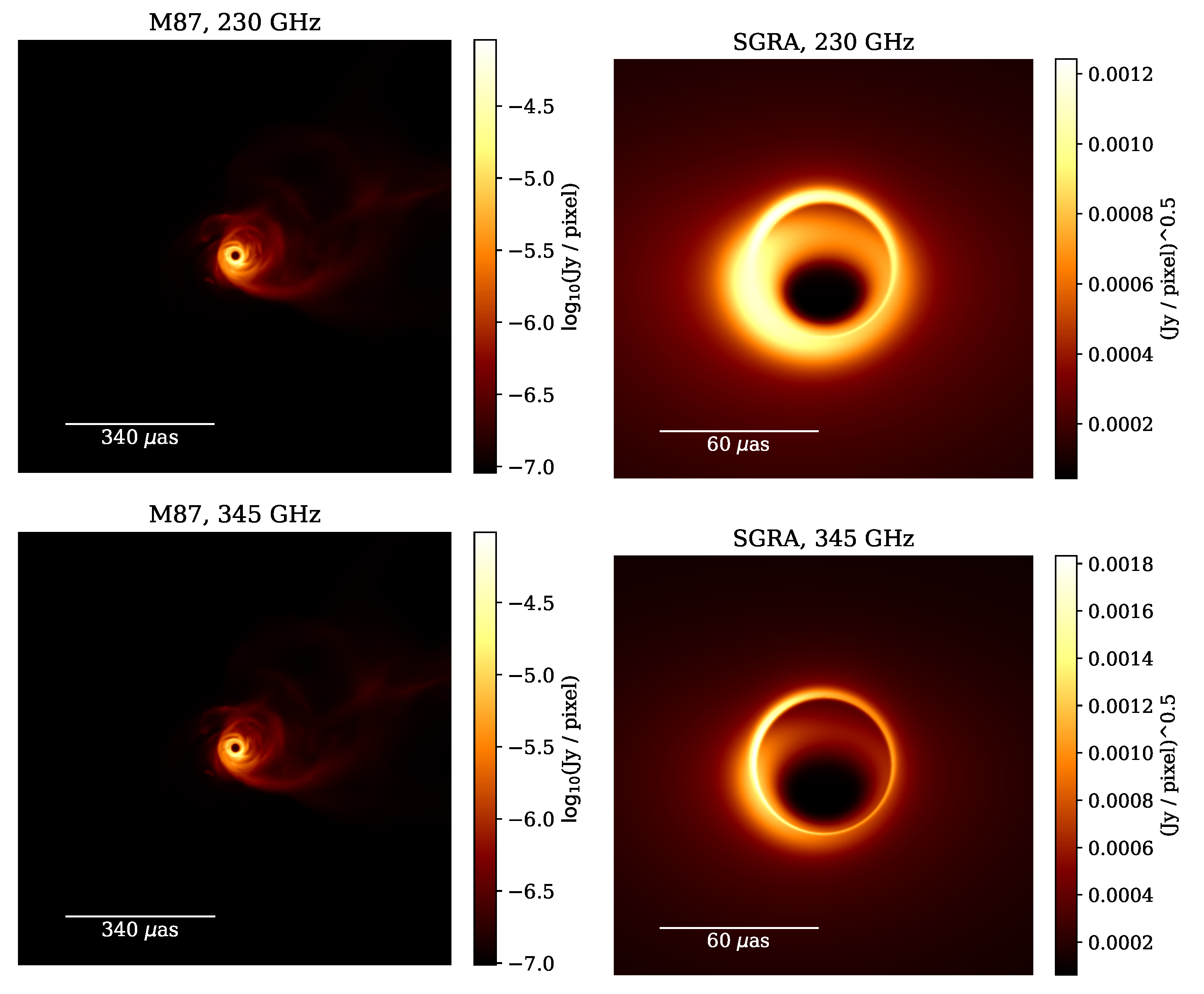
4.2. Source Models
4.2.1. M87
4.2.2. Sgr A*
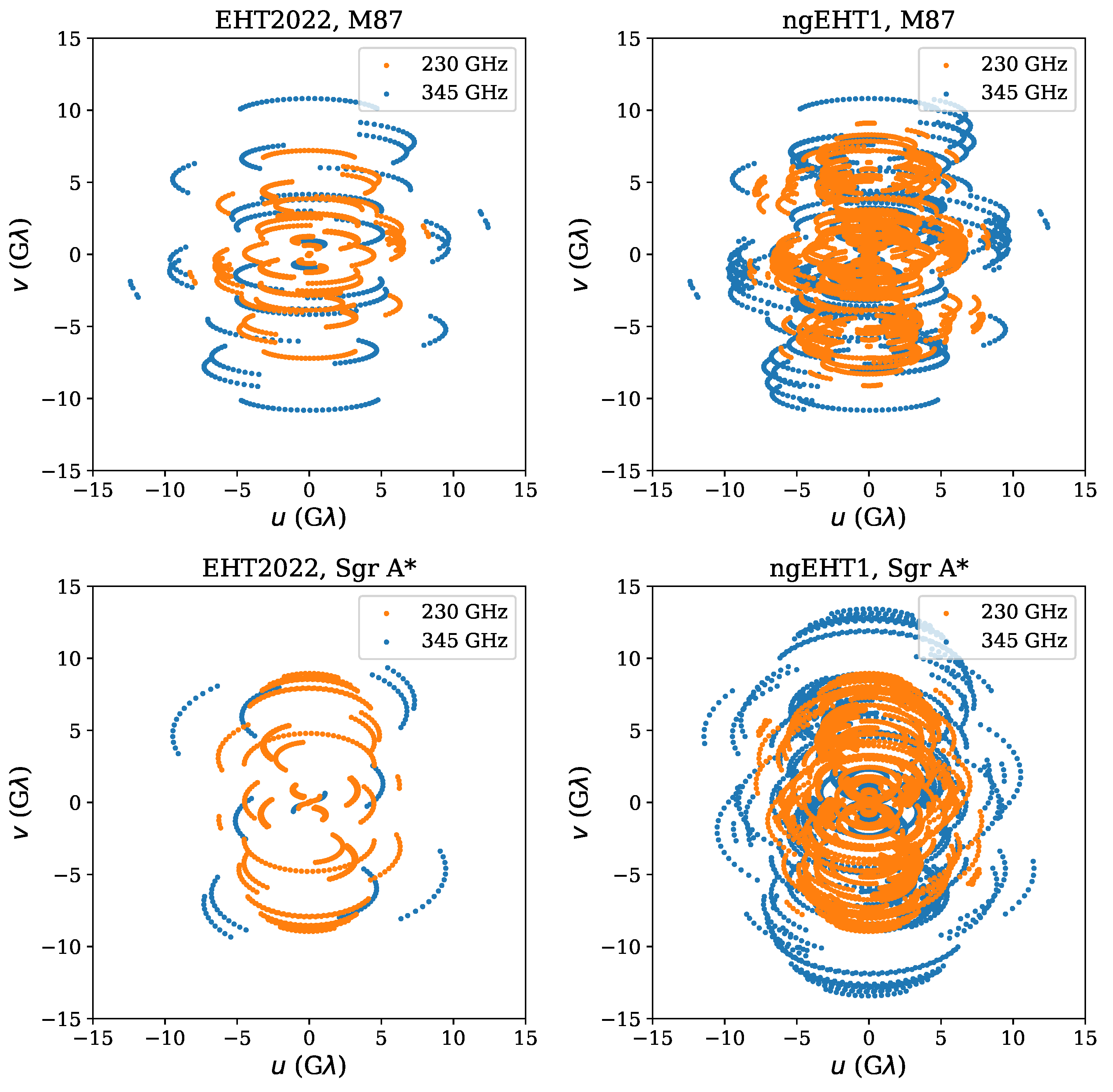
4.3. Synthetic Data
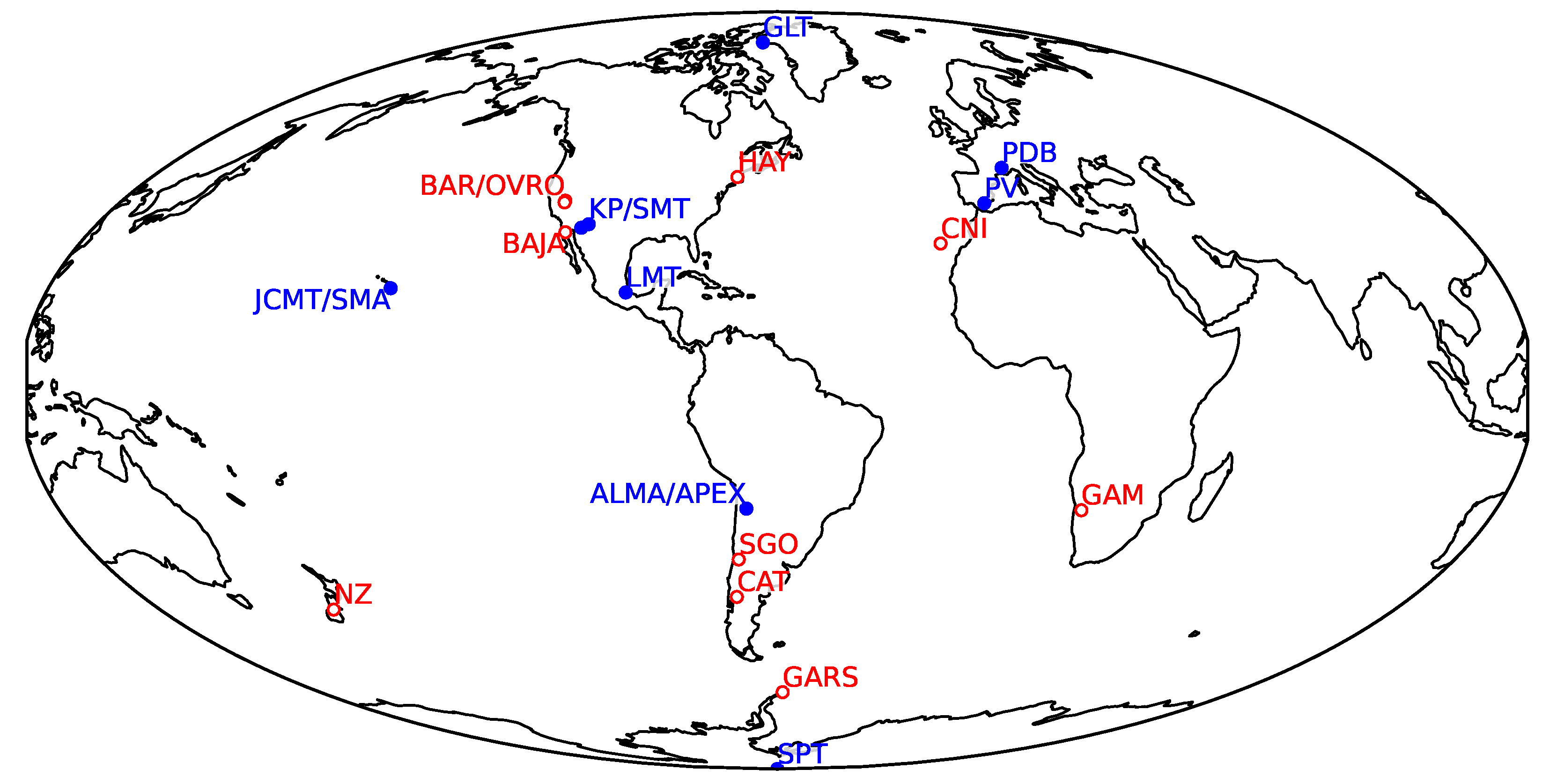
4.3.1. Station Locations
4.3.2. Data Properties
- Receiver temperature: 60 K for 230 GHz; 100 K for 345 GHz
- Aperture efficiency: 0.68 for 230 GHz; 0.42 for 345 GHz
- Bandwidth: 8 GHz
- Quantization efficiency: 0.88
- Dish diameter: 6 m for new sites, actual diameter for existing sites
- Opacity: median values in April as extracted from the MERRA-2 data by Raymond et al. [67], at 30-degree elevation. The opacities were set constant throughout and across the different datasets but are frequency-dependent.
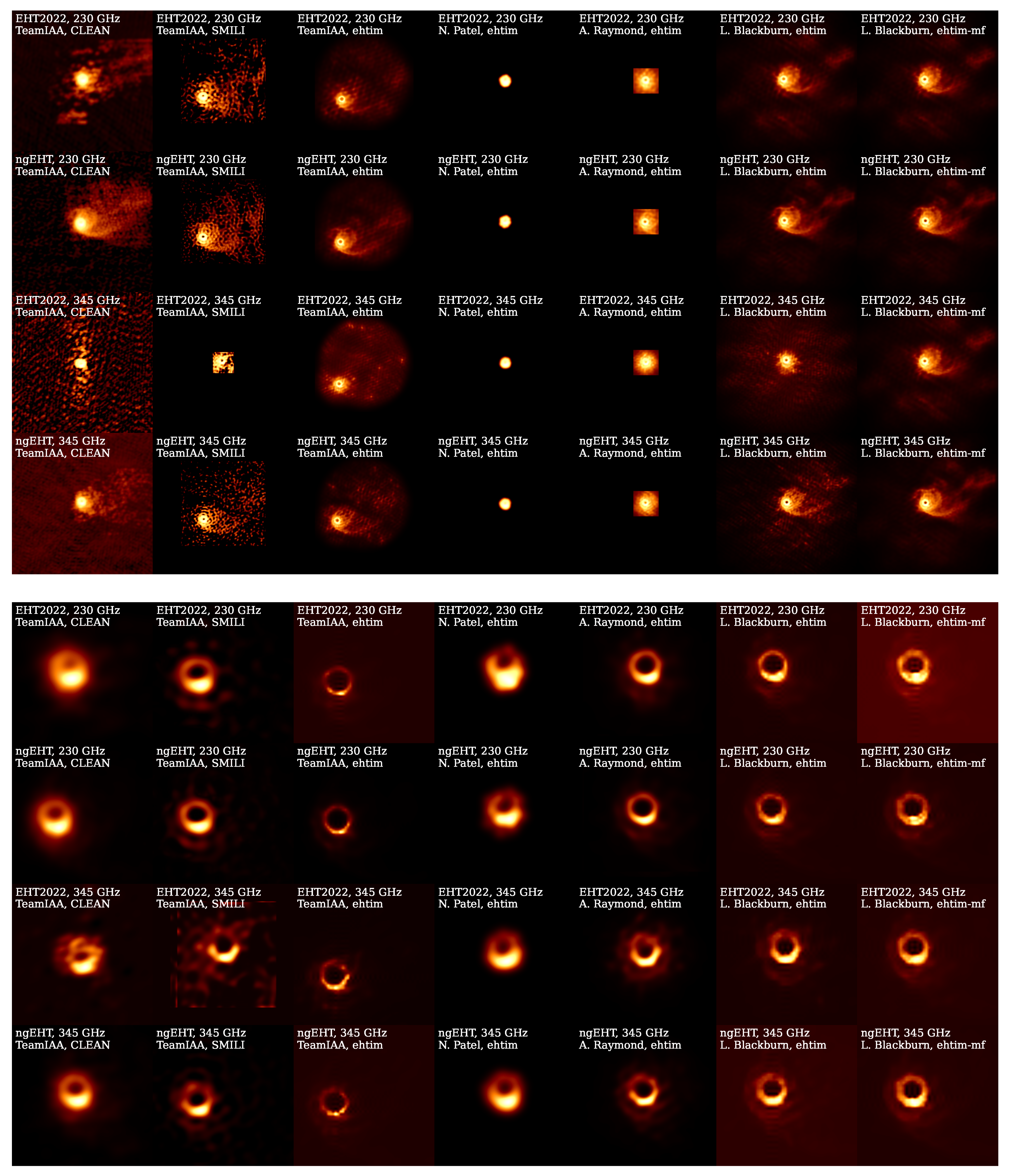
4.4. Results
5. Challenge 2
5.1. Rationale and Charge
5.2. Source Models
5.2.1. M87
5.2.2. Sgr A*
5.3. Synthetic Data
5.4. Results
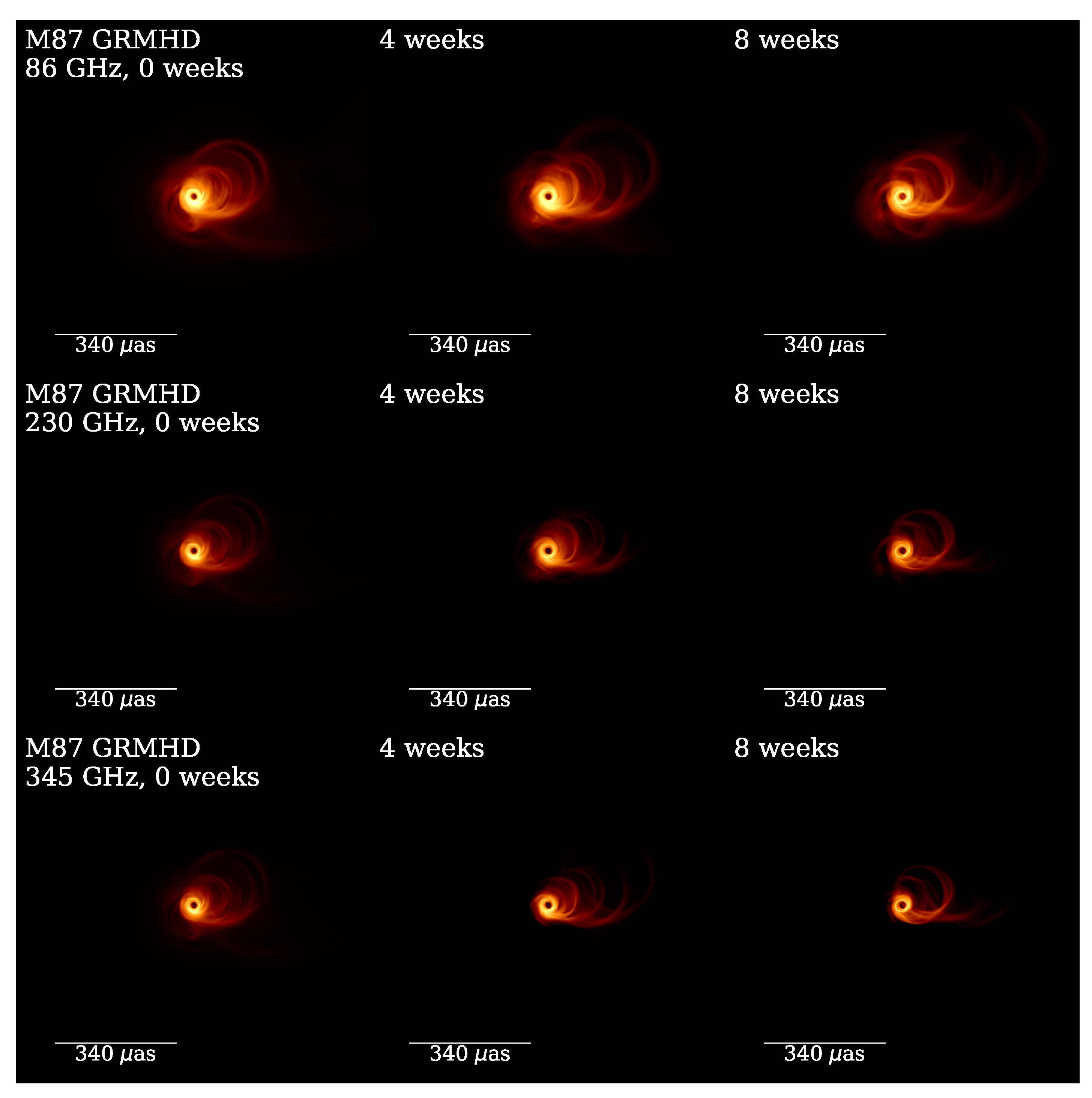
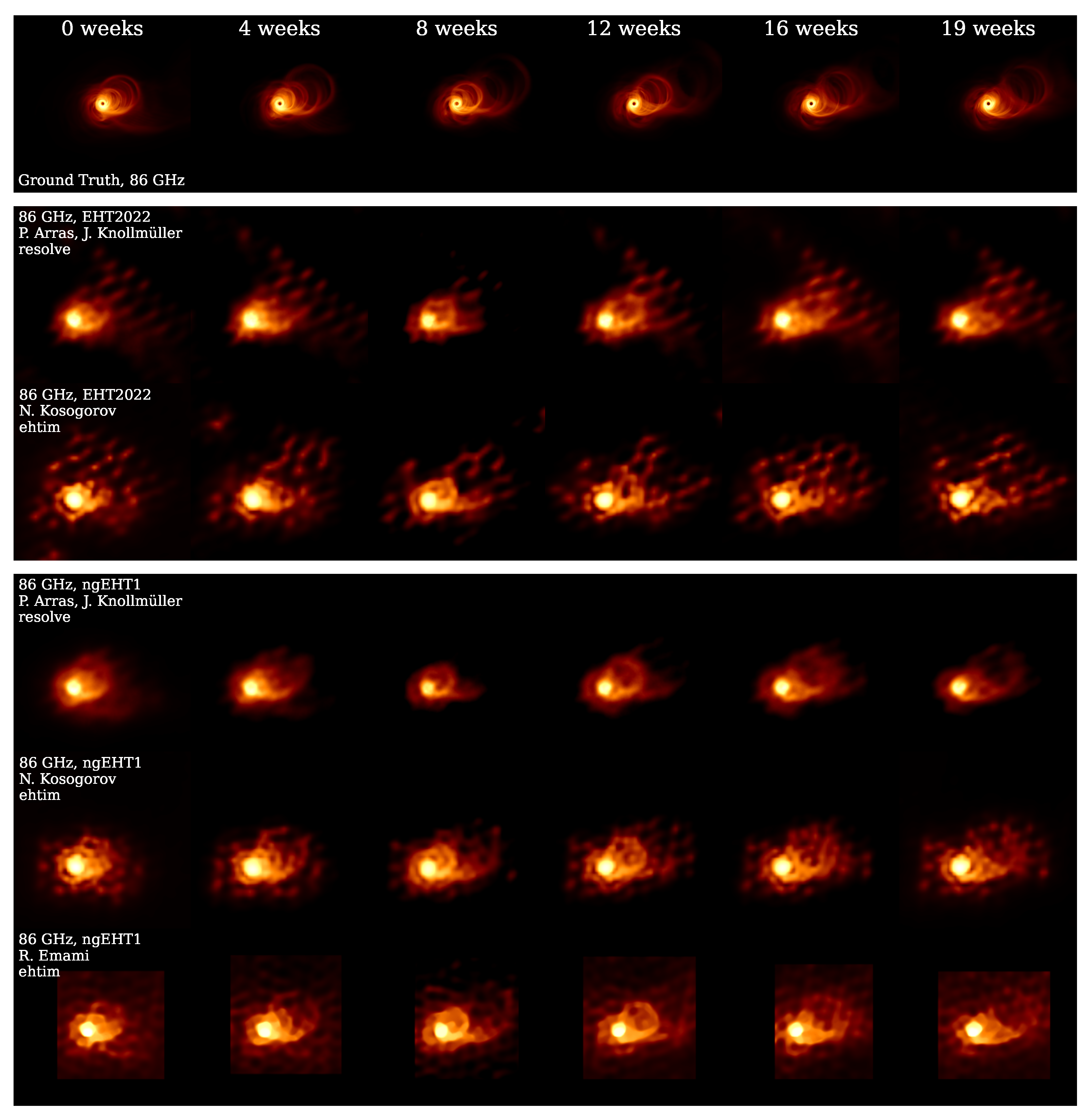
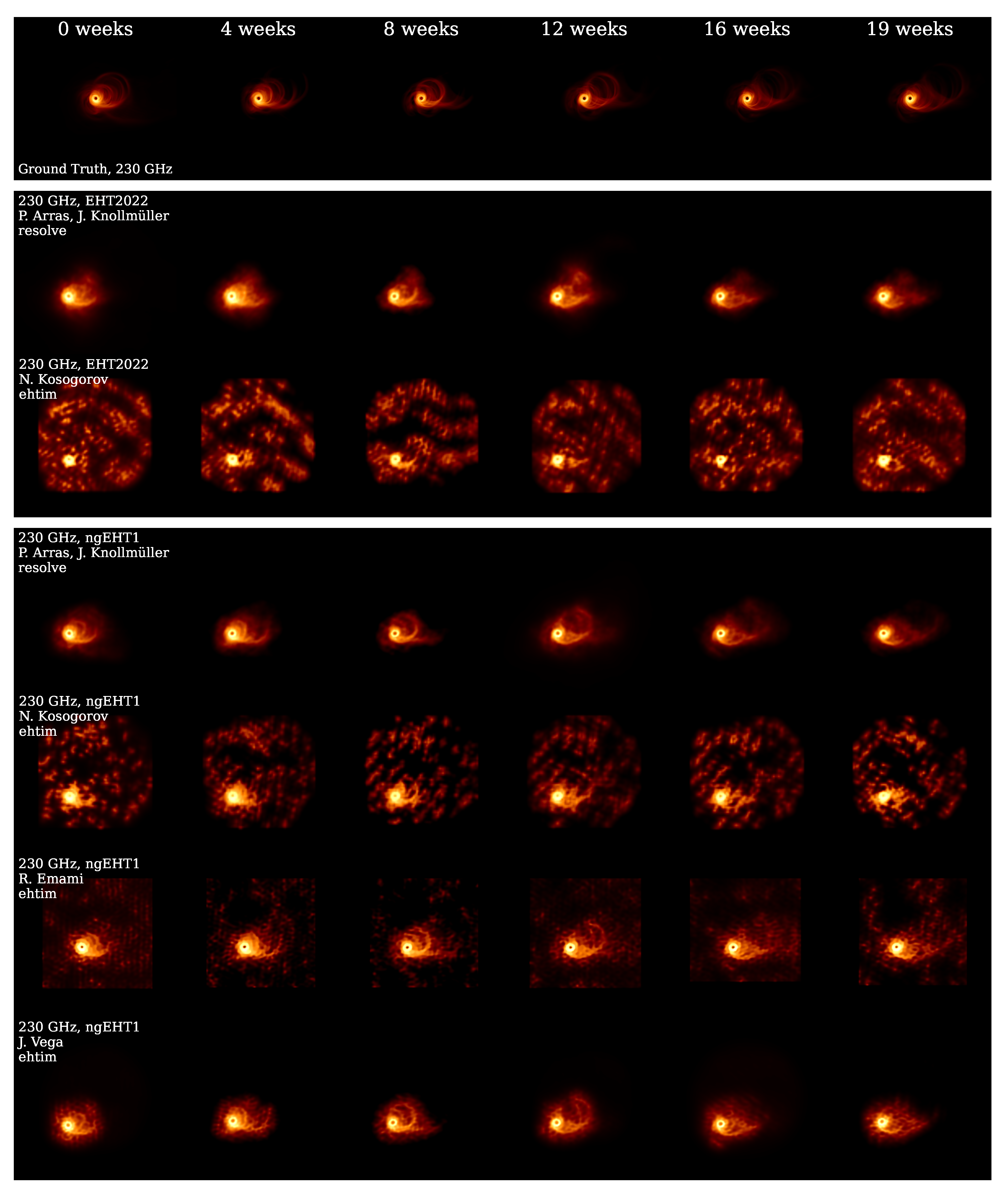
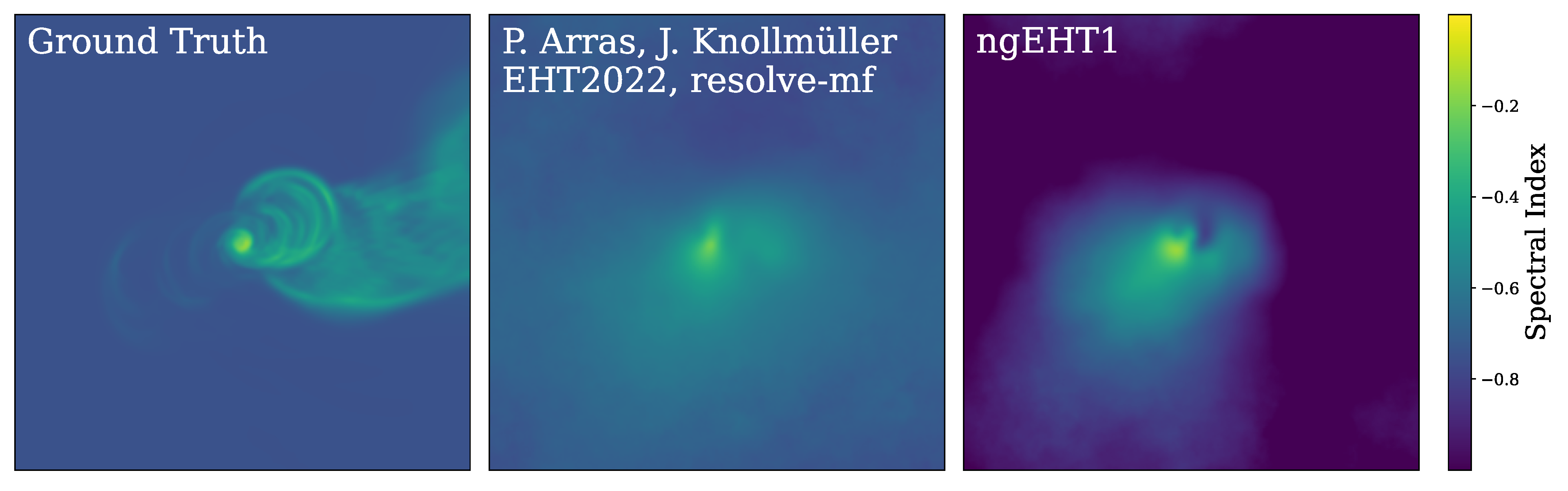
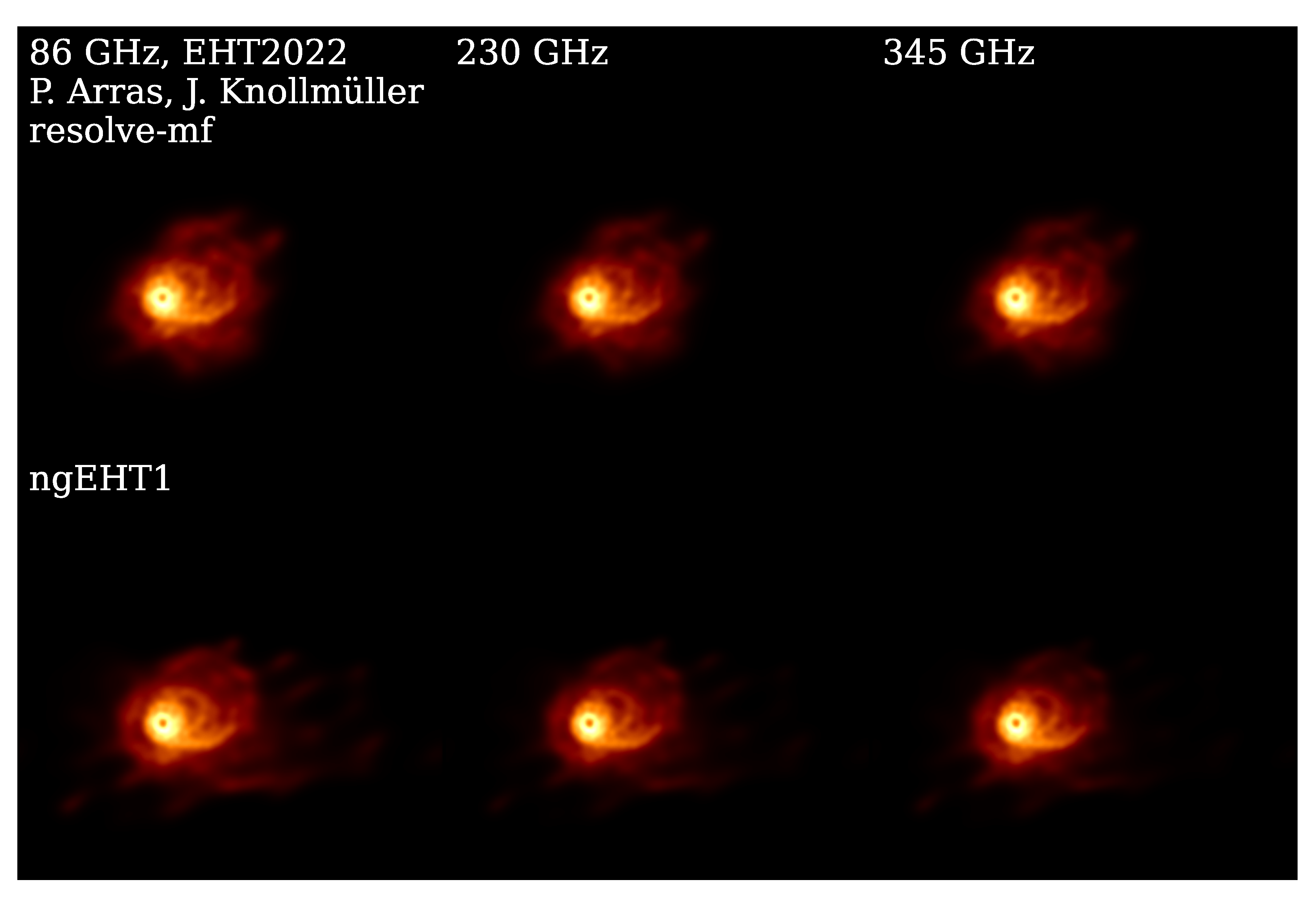
5.4.1. M87 GRMHD
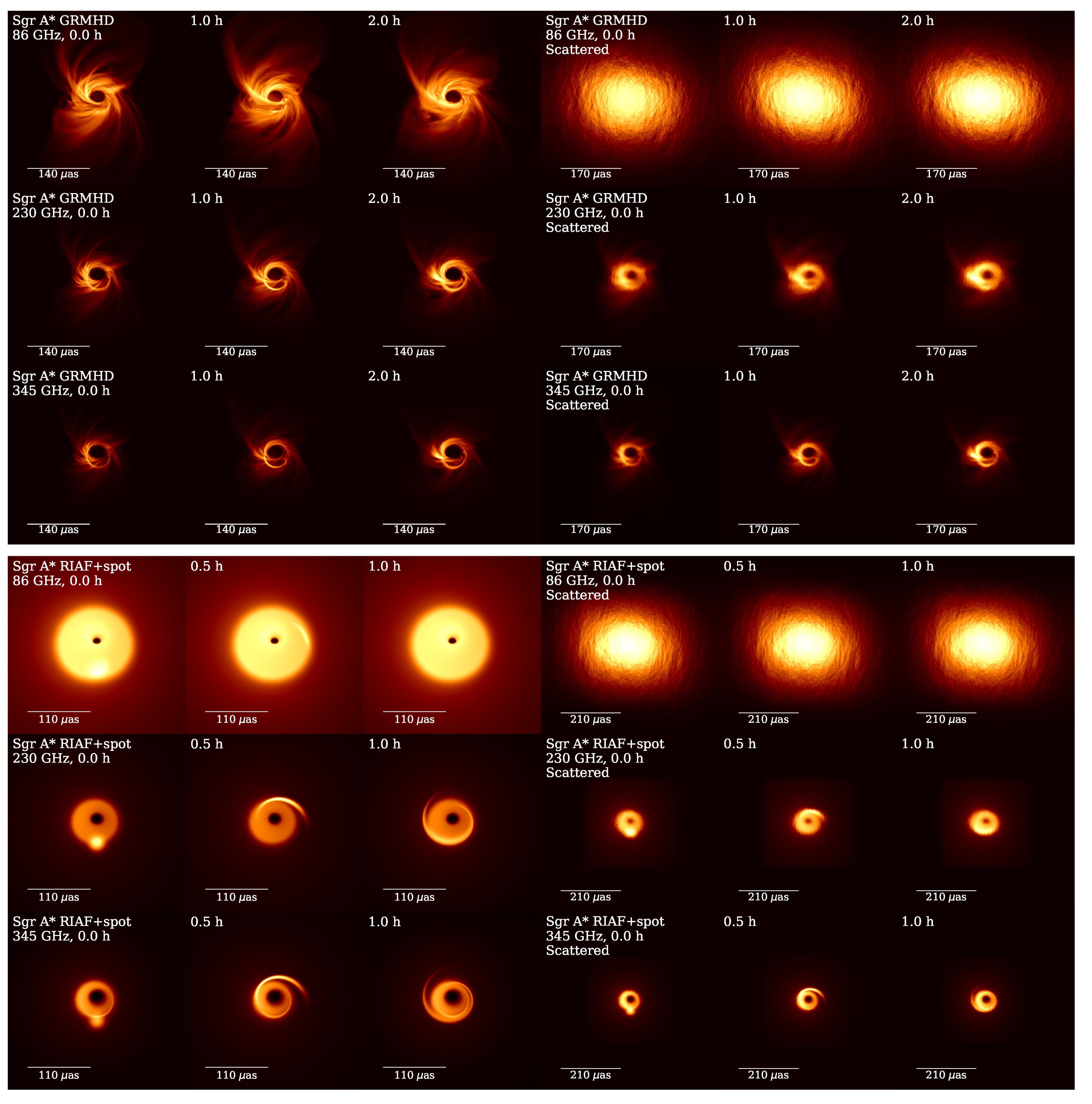
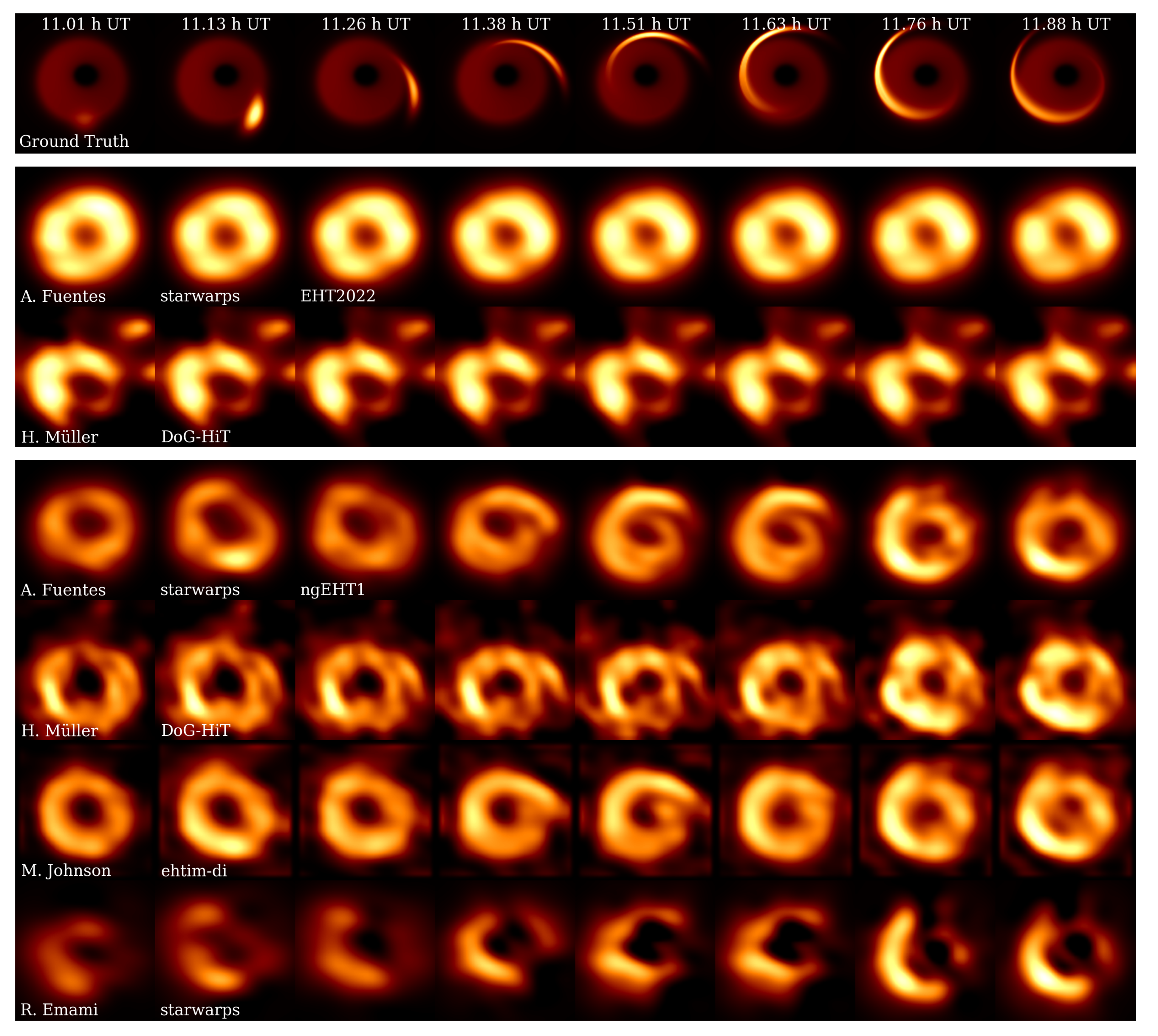
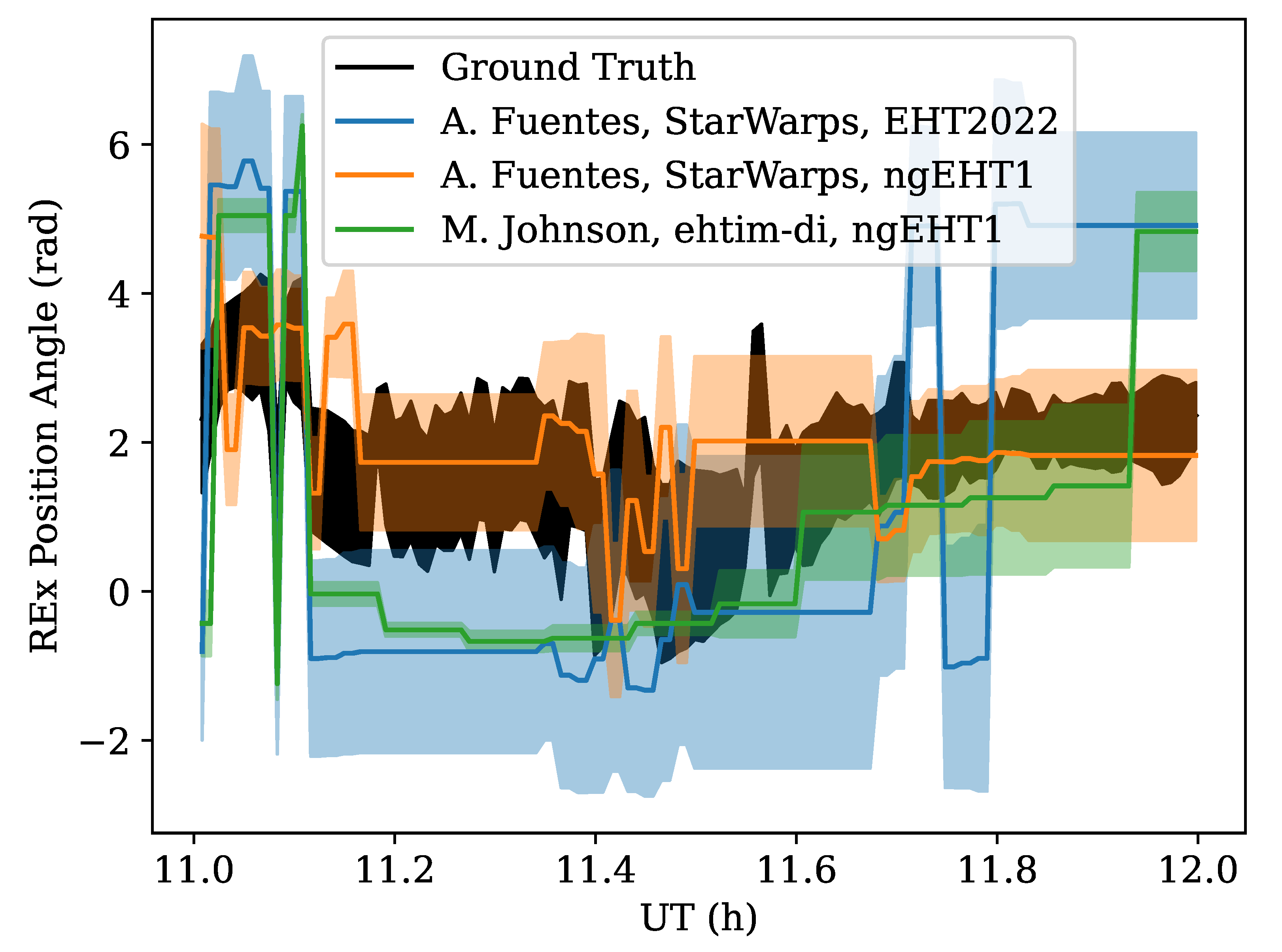
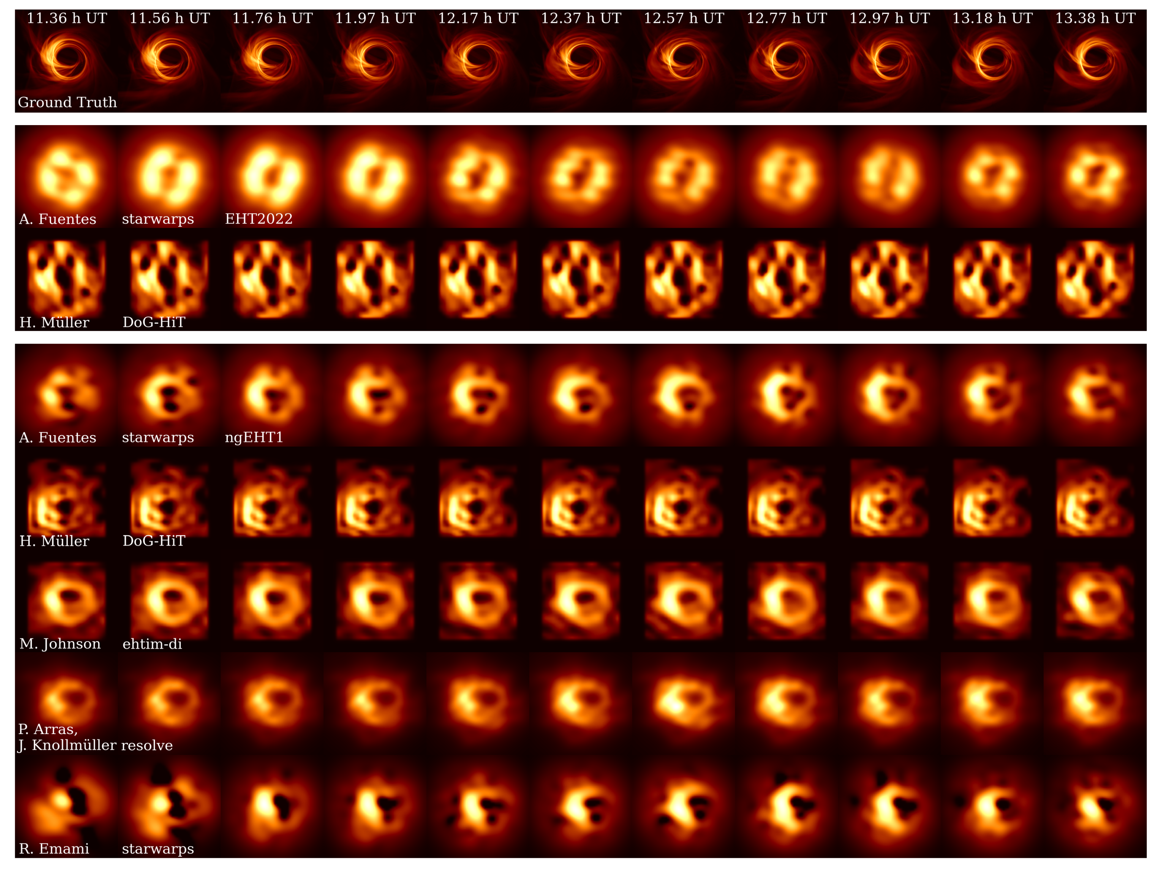
5.4.2. Sgr A* RIAF+hotspot
5.4.3. Sgr A* GRMHD
6. Conclusions and Outlook
Author Contributions
Funding
Data Availability Statement
Conflicts of Interest
| 1 | https://challenge.ngeht.org/ (accessed on 19 December 2022) |
| 2 | https://gitlab.mpcdf.mpg.de/ift/resolve (accessed on 19 December 2022) |
| 3 | https://challenge.ngeht.org/challenge3/ (accessed on 19 December 2022). |
References
- Doeleman, S.; Blackburn, L.; Dexter, J.; Gomez, J.L.; Johnson, M.D.; Palumbo, D.C.; Weintroub, J.; Farah, J.R.; Fish, V.; Loinard, L.; et al. Studying Black Holes on Horizon Scales with VLBI Ground Arrays. Proc. Bull. Am. Astron. Soc. 2019, 51, 256. [Google Scholar]
- Doeleman, S. Reference Array and Design Consideration for the next-generation Event Horizon Telescope. Galaxies 2023. in prep. [Google Scholar]
- Event Horizon Telescope Collaboration; Akiyama, K.; Alberdi, A.; Alef, W.; Asada, K.; Azulay, R.; Baczko, A.K.; Ball, D.; Baloković, M.; Barrett, J.; et al. First M87 Event Horizon Telescope Results. I. The Shadow of the Supermassive Black Hole. Astrophys. J. Lett. 2019, 875, L1. [Google Scholar] [CrossRef]
- Event Horizon Telescope Collaboration; Akiyama, K.; Alberdi, A.; Alef, W.; Asada, K.; Azulay, R.; Baczko, A.K.; Ball, D.; Baloković, M.; Barrett, J.; et al. First M87 Event Horizon Telescope Results. II. Array and Instrumentation. Astrophys. J. Lett. 2019, 875, L2. [Google Scholar] [CrossRef]
- Event Horizon Telescope Collaboration; Akiyama, K.; Alberdi, A.; Alef, W.; Asada, K.; Azulay, R.; Baczko, A.K.; Ball, D.; Baloković, M.; Barrett, J.; et al. First M87 Event Horizon Telescope Results. III. Data Processing and Calibration. Astrophys. J. Lett. 2019, 875, L3. [Google Scholar] [CrossRef]
- Event Horizon Telescope Collaboration; Akiyama, K.; Alberdi, A.; Alef, W.; Asada, K.; Azulay, R.; Baczko, A.K.; Ball, D.; Baloković, M.; Barrett, J.; et al. First M87 Event Horizon Telescope Results. IV. Imaging the Central Supermassive Black Hole. Astrophys. J. Lett. 2019, 875, L4. [Google Scholar] [CrossRef]
- Event Horizon Telescope Collaboration; Akiyama, K.; Alberdi, A.; Alef, W.; Asada, K.; Azulay, R.; Baczko, A.K.; Ball, D.; Baloković, M.; Barrett, J.; et al. First M87 Event Horizon Telescope Results. V. Physical Origin of the Asymmetric Ring. Astrophys. J. Lett. 2019, 875, L5. [Google Scholar] [CrossRef]
- Event Horizon Telescope Collaboration; Akiyama, K.; Alberdi, A.; Alef, W.; Asada, K.; Azulay, R.; Baczko, A.K.; Ball, D.; Baloković, M.; Barrett, J.; et al. First M87 Event Horizon Telescope Results. VI. The Shadow and Mass of the Central Black Hole. Astrophys. J. Lett. 2019, 875, L6. [Google Scholar] [CrossRef]
- Event Horizon Telescope Collaboration; Akiyama, K.; Algaba, J.C.; Alberdi, A.; Alef, W.; Anantua, R.; Asada, K.; Azulay, R.; Baczko, A.K.; Ball, D.; et al. First M87 Event Horizon Telescope Results. VII. Polarization of the Ring. Astrophys. J. Lett. 2021, 910, L12. [Google Scholar] [CrossRef]
- Event Horizon Telescope Collaboration; Akiyama, K.; Algaba, J.C.; Alberdi, A.; Alef, W.; Anantua, R.; Asada, K.; Azulay, R.; Baczko, A.K.; Ball, D.; et al. First M87 Event Horizon Telescope Results. VIII. Magnetic Field Structure near The Event Horizon. Astrophys. J. Lett. 2021, 910, L13. [Google Scholar] [CrossRef]
- Event Horizon Telescope Collaboration; Akiyama, K.; Alberdi, A.; Alef, W.; Algaba, J.C.; Anantua, R.; Asada, K.; Azulay, R.; Bach, U.; Baczko, A.K.; et al. First Sagittarius A* Event Horizon Telescope Results. I. The Shadow of the Supermassive Black Hole in the Center of the Milky Way. Astrophys. J. Lett. 2022, 930, L12. [Google Scholar] [CrossRef]
- Event Horizon Telescope Collaboration; Akiyama, K.; Alberdi, A.; Alef, W.; Algaba, J.C.; Anantua, R.; Asada, K.; Azulay, R.; Bach, U.; Baczko, A.K.; et al. First Sagittarius A* Event Horizon Telescope Results. II. EHT and Multiwavelength Observations, Data Processing, and Calibration. Astrophys. J. Lett. 2022, 930, L13. [Google Scholar] [CrossRef]
- Event Horizon Telescope Collaboration; Akiyama, K.; Alberdi, A.; Alef, W.; Algaba, J.C.; Anantua, R.; Asada, K.; Azulay, R.; Bach, U.; Baczko, A.K.; et al. First Sagittarius A* Event Horizon Telescope Results. III. Imaging of the Galactic Center Supermassive Black Hole. Astrophys. J. Lett. 2022, 930, L14. [Google Scholar] [CrossRef]
- Event Horizon Telescope Collaboration; Akiyama, K.; Alberdi, A.; Alef, W.; Algaba, J.C.; Anantua, R.; Asada, K.; Azulay, R.; Bach, U.; Baczko, A.K.; et al. First Sagittarius A* Event Horizon Telescope Results. IV. Variability, Morphology, and Black Hole Mass. Astrophys. J. Lett. 2022, 930, L15. [Google Scholar] [CrossRef]
- Event Horizon Telescope Collaboration; Akiyama, K.; Alberdi, A.; Alef, W.; Algaba, J.C.; Anantua, R.; Asada, K.; Azulay, R.; Bach, U.; Baczko, A.K.; et al. First Sagittarius A* Event Horizon Telescope Results. V. Testing Astrophysical Models of the Galactic Center Black Hole. Astrophys. J. Lett. 2022, 930, L16. [Google Scholar] [CrossRef]
- Event Horizon Telescope Collaboration; Akiyama, K.; Alberdi, A.; Alef, W.; Algaba, J.C.; Anantua, R.; Asada, K.; Azulay, R.; Bach, U.; Baczko, A.K.; et al. First Sagittarius A* Event Horizon Telescope Results. VI. Testing the Black Hole Metric. Astrophys. J. Lett. 2022, 930, L17. [Google Scholar] [CrossRef]
- Issaoun, S.; Pesce, D.W.; Roelofs, F.; Chael, A.; Dodson, R.; Rioja, M.J.; Akiyama, K.; Aran, R.; Blackburn, L.; Doeleman, S.S.; et al. Enabling transformational ngEHT science via the inclusion of 86 GHz capabilities. Galaxies 2023. submitted. [Google Scholar]
- Pesce, D.W.; Palumbo, D.C.M.; Narayan, R.; Blackburn, L.; Doeleman, S.S.; Johnson, M.D.; Ma, C.P.; Nagar, N.M.; Natarajan, P.; Ricarte, A. Toward Determining the Number of Observable Supermassive Black Hole Shadows. Astrophys. J. Lett. 2021, 923, 260. [Google Scholar] [CrossRef]
- Pesce, D.W.; Palumbo, D.C.M.; Ricarte, A.; Broderick, A.E.; Johnson, M.D.; Nagar, N.M.; Natarajan, P.; Gómez, J.L. Expectations for Horizon-Scale Supermassive Black Hole Population Studies with the ngEHT. Galaxies 2022, 10, 109. [Google Scholar] [CrossRef]
- Bouman, K.L. Extreme Imaging via Physical Model Inversion: Seeing around Corners and Imaging Black Holes. Ph.D. Thesis, Massachusetts Institute of Technology, Cambridge, MA, USA, 2017. [Google Scholar]
- Chatterjee, K.; Chael, A.; Tiede, P.; Mizuno, Y.; Emami, R.; Fromm, C.; Ricarte, A.; Blackburn, L.; Roelofs, F.; Johnson, M.D.; et al. Comparing accretion flow morphology in numerical simulations of black holes from the ngEHT Model Library: The impact of radiation physics. arXiv 2022, arXiv:2212.01804. [Google Scholar]
- Högbom, J.A. Aperture Synthesis with a Non-Regular Distribution of Interferometer Baselines. Astron. Astrophys. Suppl. Ser. 1974, 15, 417. [Google Scholar]
- Wilkinson, P.N.; Readhead, A.C.S.; Purcell, G.H.; Anderson, B. Radio structure of 3C 147 determined by multi-element very long baseline interferometry. Nature 1977, 269, 764–768. [Google Scholar] [CrossRef]
- Cornwell, T.J. Hogbom’s CLEAN algorithm. Impact on astronomy and beyond. Commentary on: Högbom J. A., 1974, A&AS, 15, 417. Astron. Astrophys. 2009, 500, 65–66. [Google Scholar] [CrossRef]
- Shepherd, M.C.; Pearson, T.J.; Taylor, G.B. DIFMAP: An interactive program for synthesis imaging. Proc. Bull. Am. Astron. Soc. 1995, 27, 903. [Google Scholar]
- Frieden, B.R. Restoring with Maximum Likelihood and Maximum Entropy. J. Opt. Soc. Am. 1972, 62, 511–518. [Google Scholar] [CrossRef] [PubMed]
- Coughlan, C.P.; Gabuzda, D.C. High resolution VLBI polarization imaging of AGN with the maximum entropy method. Mon. Not. R. Astron. Soc. 2016, 463, 1980–2001. [Google Scholar] [CrossRef] [Green Version]
- Narayan, R.; Nityananda, R. Maximum Entropy Image Restoration in Astronomy. Annu. Rev. Astron. Astrophys. 1986, 24, 127–170. [Google Scholar] [CrossRef]
- Chael, A.A.; Johnson, M.D.; Bouman, K.L.; Blackburn, L.L.; Akiyama, K.; Narayan, R. Interferometric Imaging Directly with Closure Phases and Closure Amplitudes. Astrophys. J. 2018, 857, 23. [Google Scholar] [CrossRef]
- Chael, A.A.; Johnson, M.D.; Narayan, R.; Doeleman, S.S.; Wardle, J.F.C.; Bouman, K.L. High-resolution Linear Polarimetric Imaging for the Event Horizon Telescope. Astrophys. J. 2016, 829, 11. [Google Scholar] [CrossRef]
- Akiyama, K.; Kuramochi, K.; Ikeda, S.; Fish, V.L.; Tazaki, F.; Honma, M.; Doeleman, S.S.; Broderick, A.E.; Dexter, J.; Mościbrodzka, M.; et al. Imaging the Schwarzschild-radius-scale Structure of M87 with the Event Horizon Telescope Using Sparse Modeling. Astrophys. J. 2017, 838, 1. [Google Scholar] [CrossRef]
- Akiyama, K.; Ikeda, S.; Pleau, M.; Fish, V.L.; Tazaki, F.; Kuramochi, K.; Broderick, A.E.; Dexter, J.; Mościbrodzka, M.; Gowanlock, M.; et al. Superresolution Full-polarimetric Imaging for Radio Interferometry with Sparse Modeling. Astrophys. J. 2017, 153, 159. [Google Scholar] [CrossRef] [Green Version]
- Chael, A.A.; Bouman, K.L.; Johnson, M.D.; Narayan, R.; Doeleman, S.S.; Wardle, J.F.C.; Blackburn, L.L.; Akiyama, K.; Wielgus, M.; Chan, C.k.; et al. ehtim: Imaging, analysis, and simulation software for radio interferometry. Astrophys. Source Code Libr. 2019, ascl-1904. [Google Scholar]
- Chael, A.; Issaoun, S.; Pesce, D.W.; Johnson, M.D.; Ricarte, A.; Fromm, C.M.; Mizuno, Y. Multi-frequency Black Hole Imaging for the Next-Generation Event Horizon Telescope. arXiv 2022, arXiv:2210.12226. [Google Scholar]
- Johnson, M.D.; Narayan, R.; Psaltis, D.; Blackburn, L.; Kovalev, Y.Y.; Gwinn, C.R.; Zhao, G.Y.; Bower, G.C.; Moran, J.M.; Kino, M.; et al. The Scattering and Intrinsic Structure of Sagittarius A* at Radio Wavelengths. Astrophys. J. 2018, 865, 104. [Google Scholar] [CrossRef] [Green Version]
- Johnson, M.D.; Lupsasca, A.; Strominger, A.; Wong, G.N.; Hadar, S.; Kapec, D.; Narayan, R.; Chael, A.; Gammie, C.F.; Galison, P.; et al. Universal interferometric signatures of a black hole’s photon ring. Sci. Adv. 2020, 6, eaaz1310. [Google Scholar] [CrossRef] [PubMed] [Green Version]
- Byrd, R.H.; Lu, P.; Nocedal, J. A Limited Memory Algorithm for Bound Constrained Optimization. SIAM J. Sci. Stat. Comput. 1995, 16, 1190–1208. [Google Scholar] [CrossRef]
- Jones, E.; Oliphant, T.; Peterson, P. SciPy: Open Source Scientific Tools for Python. 2001. Available online: https://github.com/takluyver/scipy.org-new/blob/master/www/scipylib/citing.rst (accessed on 25 August 2015).
- Bouman, K.L.; Johnson, M.D.; Dalca, A.V.; Chael, A.A.; Roelofs, F.; Doeleman, S.S.; Freeman, W.T. Reconstructing Video from Interferometric Measurements of Time-Varying Sources. arXiv 2017, arXiv:1711.01357. [Google Scholar] [CrossRef] [Green Version]
- Emami, R.; Tiede, P.; Doeleman, S.S.; Roelofs, F.; Wielgus, M.; Blackburn, L.; Liska, M.; Chatterjee, K.; Ripperda, B.; Fuentes, A.; et al. Tracing the hot spot motion using the next generation Event Horizon Telescope (ngEHT). arXiv 2022, arXiv:2211.06773. [Google Scholar]
- Arras, P.; Bester, H.L.; Perley, R.A.; Leike, R.; Smirnov, O.; Westermann, R.; Enßlin, T.A. Comparison of classical and Bayesian imaging in radio interferometry. Astron. Astrophys. 2021, 646, A84. [Google Scholar] [CrossRef]
- Arras, P.; Frank, P.; Haim, P.; Knollmüller, J.; Leike, R.; Reinecke, M.; Enßlin, T. Variable structures in M87* from space, time and frequency d interferometry. Nat. Astron. 2022, 6, 259–269. [Google Scholar] [CrossRef]
- Knollmüller, J.; Enßlin, T.A. Metric Gaussian Variational Inference. arXiv 2019, arXiv:1901.11033. [Google Scholar]
- Arras, P.; Reinecke, M.; Westermann, R.; Enßin, T.A. Efficient wide-field radio interferometry response. Astron. Astrophys. 2021, 646, A58. [Google Scholar] [CrossRef]
- Müller, H.; Lobanov, A.P. DoG-HiT: A novel VLBI multiscale imaging approach. Astron. Astrophys. 2022, 666, A137. [Google Scholar] [CrossRef]
- Müller, H.; Lobanov, A. Multi-scale and Multi-directional VLBI Imaging with CLEAN. Astron. Astrophys. 2022. submitted. [Google Scholar]
- Müller, H.; Lobanov, A. Dynamic polarimetry with the multiresolution support. Astron. Astrophys. 2022. submitted. [Google Scholar]
- Thompson, A.R.; Moran, J.M.; Swenson, G.W., Jr. Interferometry and Synthesis in Radio Astronomy, 3rd ed.; Springer Nature: Berlin/Heidelberg, Germany, 2017. [Google Scholar] [CrossRef] [Green Version]
- Bustamante, S.; Blackburn, L.; Narayanan, G.; Schloerb, F.P.; Hughes, D. The Role of the Large Millimeter Telescope in Black Hole Science with the Next-Generation Event Horizon Telescope. Galaxies 2023, 11, 2. [Google Scholar] [CrossRef]
- Mizuno, Y.; Fromm, C.M.; Younsi, Z.; Porth, O.; Olivares, H.; Rezzolla, L. Comparison of the ion-to-electron temperature ratio prescription: GRMHD simulations with electron thermodynamics. Mon. Not. R. Astron. Soc. 2021, 506, 741–758. [Google Scholar] [CrossRef]
- Porth, O.; Olivares, H.; Mizuno, Y.; Younsi, Z.; Rezzolla, L.; Moscibrodzka, M.; Falcke, H.; Kramer, M. The black hole accretion code. Comput. Astrophys. Cosmol. 2017, 4, 1. [Google Scholar] [CrossRef]
- Tchekhovskoy, A.; McKinney, J.C. Prograde and retrograde black holes: Whose jet is more powerful? Mon. Not. R. Astron. Soc. Lett. 2012, 423, L55–L59. [Google Scholar] [CrossRef]
- Younsi, Z.; Wu, K.; Fuerst, S.V. General relativistic radiative transfer: Formulation and emission from structured tori around black holes. Astron. Astrophys. 2012, 545, A13. [Google Scholar] [CrossRef] [Green Version]
- Younsi, Z.; Porth, O.; Mizuno, Y.; Fromm, C.M.; Olivares, H. Modelling the polarised emission from black holes on event horizon-scales. In Proceedings of the Perseus in Sicily: From Black Hole to Cluster Outskirts; Asada, K., de Gouveia Dal Pino, E., Giroletti, M., Nagai, H., Nemmen, R., Eds.; Cambridge University Press: Cambridge, UK, 2020; Volume 342, pp. 9–12. [Google Scholar] [CrossRef] [Green Version]
- Pandya, A.; Zhang, Z.; Chandra, M.; Gammie, C.F. Polarized Synchrotron Emissivities and Absorptivities for Relativistic Thermal, Power-law, and Kappa Distribution Functions. Astrophys. J. 2016, 822, 34. [Google Scholar] [CrossRef] [Green Version]
- Ball, D.; Sironi, L.; Özel, F. Electron and Proton Acceleration in Trans-relativistic Magnetic Reconnection: Dependence on Plasma Beta and Magnetization. Astrophys. J. 2018, 862, 80. [Google Scholar] [CrossRef] [Green Version]
- Davelaar, J.; Olivares, H.; Porth, O.; Bronzwaer, T.; Janssen, M.; Roelofs, F.; Mizuno, Y.; Fromm, C.M.; Falcke, H.; Rezzolla, L. Modeling non-thermal emission from the jet-launching region of M 87 with adaptive mesh refinement. Astron. Astrophys. 2019, 632, A2. [Google Scholar] [CrossRef] [Green Version]
- Fromm, C.M.; Cruz-Osorio, A.; Mizuno, Y.; Nathanail, A.; Younsi, Z.; Porth, O.; Olivares, H.; Davelaar, J.; Falcke, H.; Kramer, M.; et al. Impact of non-thermal particles on the spectral and structural properties of M87. Astron. Astrophys. 2022, 660, A107. [Google Scholar] [CrossRef]
- Broderick, A.E.; Loeb, A. Imaging optically-thin hotspots near the black hole horizon of Sgr A* at radio and near-infrared wavelengths. Mon. Not. R. Astron. Soc. 2006, 367, 905–916. [Google Scholar] [CrossRef]
- Pu, H.Y.; Broderick, A.E. Probing the Innermost Accretion Flow Geometry of Sgr A* with Event Horizon Telescope. Astrophys. J. 2018, 863, 148. [Google Scholar] [CrossRef]
- Tiede, P.; Pu, H.Y.; Broderick, A.E.; Gold, R.; Karami, M.; Preciado-López, J.A. Spacetime Tomography Using the Event Horizon Telescope. Astrophys. J. 2020, 892, 132. [Google Scholar] [CrossRef]
- Zhao, J.H.; Young, K.H.; Herrnstein, R.M.; Ho, P.T.P.; Tsutsumi, T.; Lo, K.Y.; Goss, W.M.; Bower, G.C. Variability of Sagittarius A*: Flares at 1 Millimeter. Astrophys. J. 2003, 586, L29–L32. [Google Scholar] [CrossRef] [Green Version]
- Bower, G.C.; Dexter, J.; Markoff, S.; Gurwell, M.A.; Rao, R.; McHardy, I. A Black Hole Mass-Variability Timescale Correlation at Submillimeter Wavelengths. Astrophys. J. Lett. 2015, 811, L6. [Google Scholar] [CrossRef] [Green Version]
- Bower, G.C.; Dexter, J.; Asada, K.; Brinkerink, C.D.; Falcke, H.; Ho, P.; Inoue, M.; Markoff, S.; Marrone, D.P.; Matsushita, S.; et al. ALMA Observations of the Terahertz Spectrum of Sagittarius A*. Astrophys. J. Lett. 2019, 881, L2. [Google Scholar] [CrossRef]
- Liu, H.B.; Wright, M.C.H.; Zhao, J.H.; Brinkerink, C.D.; Ho, P.T.P.; Mills, E.A.C.; Martín, S.; Falcke, H.; Matsushita, S.; Martí-Vidal, I. Linearly polarized millimeter and submillimeter continuum emission of Sgr A* constrained by ALMA. Astron. Astrophys. 2016, 593, A107. [Google Scholar] [CrossRef] [Green Version]
- Gravity Collaboration; Abuter, R.; Amorim, A.; Bauböck, M.; Berger, J.P.; Bonnet, H.; Brandner, W.; Clénet, Y.; Coudé Du Foresto, V.; de Zeeuw, P.T.; et al. A geometric distance measurement to the Galactic center black hole with 0.3% uncertainty. Astron. Astrophys. 2019, 625, L10. [Google Scholar] [CrossRef] [Green Version]
- Raymond, A.W.; Palumbo, D.; Paine, S.N.; Blackburn, L.; Córdova Rosado, R.; Doeleman, S.S.; Farah, J.R.; Johnson, M.D.; Roelofs, F.; Tilanus, R.P.J.; et al. Evaluation of New Submillimeter VLBI Sites for the Event Horizon Telescope. Astrophys. J. Suppl. Ser. 2021, 253, 5. [Google Scholar] [CrossRef]
- Wielgus, M.; Moscibrodzka, M.; Vos, J.; Gelles, Z.; Martí-Vidal, I.; Farah, J.; Marchili, N.; Goddi, C.; Messias, H. Orbital motion near Sagittarius A*. Constraints from polarimetric ALMA observations. Astron. Astrophys. 2022, 665, L6. [Google Scholar] [CrossRef]
- Liska, M.; Chatterjee, K.; Tchekhovskoy, A.; Yoon, D.; van Eijnatten, D.; Hesp, C.; Markoff, S.; Ingram, A.; van der Klis, M. H-AMR: A New GPU-accelerated GRMHD Code for Exascale Computing With 3D Adaptive Mesh Refinement and Local Adaptive Time-stepping. arXiv 2019, arXiv:1912.10192. [Google Scholar] [CrossRef]
- Mościbrodzka, M.; Gammie, C.F. IPOLE—Semi-analytic scheme for relativistic polarized radiative transport. Mon. Not. R. Astron. Soc. 2018, 475, 43–54. [Google Scholar] [CrossRef] [Green Version]
- Younsi, Z.; Psaltis, D.; Özel, F. Black Hole Images as Tests of General Relativity: Effects of Spacetime Geometry. arXiv 2021, arXiv:2111.01752. [Google Scholar] [CrossRef]
- Broderick, A.E.; Fish, V.L.; Johnson, M.D.; Rosenfeld, K.; Wang, C.; Doeleman, S.S.; Akiyama, K.; Johannsen, T.; Roy, A.L. Modeling Seven Years of Event Horizon Telescope Observations with Radiatively Inefficient Accretion Flow Models. Astrophys. J. 2016, 820, 137. [Google Scholar] [CrossRef]
- Gravity Collaboration; Abuter, R.; Amorim, A.; Anugu, N.; Bauböck, M.; Benisty, M.; Berger, J.P.; Blind, N.; Bonnet, H.; Brandner, W.; et al. Detection of the gravitational redshift in the orbit of the star S2 near the Galactic centre massive black hole. Astron. Astrophys. 2018, 615, L15. [Google Scholar] [CrossRef] [Green Version]
- Roelofs, F.; Janssen, M.; Natarajan, I.; Deane, R.; Davelaar, J.; Olivares, H.; Porth, O.; Paine, S.N.; Bouman, K.L.; Tilanus, R.P.J.; et al. SYMBA: An end-to-end VLBI synthetic data generation pipeline. Simulating Event Horizon Telescope observations of M 87. Astron. Astrophys. 2020, 636, A5. [Google Scholar] [CrossRef]
- Blecher, T.; Deane, R.; Bernardi, G.; Smirnov, O. MEQSILHOUETTE: A mm-VLBI observation and signal corruption simulator. Mon. Not. R. Astron. Soc. 2017, 464, 143–151. [Google Scholar] [CrossRef] [Green Version]
- Natarajan, I.; Deane, R.; Martí-Vidal, I.; Roelofs, F.; Janssen, M.; Wielgus, M.; Blackburn, L.; Blecher, T.; Perkins, S.; Smirnov, O.; et al. MeqSilhouette v2: Spectrally resolved polarimetric synthetic data generation for the event horizon telescope. Mon. Not. R. Astron. Soc. 2022, 512, 490–504. [Google Scholar] [CrossRef]
- Janssen, M.; Goddi, C.; van Bemmel, I.M.; Kettenis, M.; Small, D.; Liuzzo, E.; Rygl, K.; Martí-Vidal, I.; Blackburn, L.; Wielgus, M.; et al. rPICARD: A CASA-based calibration pipeline for VLBI data. Calibration and imaging of 7 mm VLBA observations of the AGN jet in M 87. Astron. Astrophys. 2019, 626, A75. [Google Scholar] [CrossRef] [Green Version]
- Gelaro, R.; McCarty, W.; Suárez, M.J.; Todling, R.; Molod, A.; Takacs, L.; Randles, C.A.; Darmenov, A.; Bosilovich, M.G.; Reichle, R.; et al. The Modern-Era Retrospective Analysis for Research and Applications, Version 2 (MERRA-2). J. Clim. 2017, 30, 5419–5454. [Google Scholar] [CrossRef]
- Paine, S. The am Atmospheric Model. 2019. Available online: https://zenodo.org/record/3406496#.Y7017nZByUk (accessed on 19 December 2022).
- Farah, J.; Galison, P.; Akiyama, K.; Bouman, K.L.; Bower, G.C.; Chael, A.; Fuentes, A.; Gómez, J.L.; Honma, M.; Johnson, M.D.; et al. Selective Dynamical Imaging of Interferometric Data. Astrophys. J. Lett. 2022, 930, L18. [Google Scholar] [CrossRef]
- Chael, A.A. Simulating and Imaging Supermassive Black Hole Accretion Flows. Ph.D. Thesis, Harvard University, Cambridge, MA, USA, 2019. [Google Scholar]
- Bella, N.L.; Issaoun, S.; Roelofs, F.; Fromm, C.; Falcke, H. Expanding Sgr A* dynamical imaging capabilities with an African extension to the Event Horizon Telescope. Astron. Astrophys. 2023. submitted. [Google Scholar]
- Chael, A.; Johnson, M.D.; Lupsasca, A. Observing the Inner Shadow of a Black Hole: A Direct View of the Event Horizon. Astrophys. J. 2021, 918, 6. [Google Scholar] [CrossRef]
- Bronzwaer, T.; Falcke, H. The Nature of Black Hole Shadows. Astrophys. J. 2021, 920, 155. [Google Scholar] [CrossRef]
- Tiede, P.; Johnson, M.D.; Pesce, D.W.; Palumbo, D.C.M.; Chang, D.O.; Galison, P. Measuring Photon Rings with the ngEHT. arXiv 2022, arXiv:2210.13498. [Google Scholar]
- Dodson, R.; Rioja, M.J.; Jung, T.; Goméz, J.L.; Bujarrabal, V.; Moscadelli, L.; Miller-Jones, J.C.A.; Tetarenko, A.J.; Sivakoff, G.R. The science case for simultaneous mm-wavelength receivers in radio astronomy. New Astron. Rev. 2017, 79, 85–102. [Google Scholar] [CrossRef] [Green Version]
- Rioja, M.J.; Dodson, R. Precise radio astrometry and new developments for the next-generation of instruments. Astron. Astrophys. Rev. 2020, 28, 6. [Google Scholar] [CrossRef]


| Source | Array | (GHz) | Submitter | Method | ||||||
|---|---|---|---|---|---|---|---|---|---|---|
| M87 | EHT2022 | 230 | L. Blackburn | ehtim | 1.1 | 1.01 | 0.93 | 0.87 | 5.4 | 856 |
| M87 | EHT2022 | 230 | L. Blackburn | ehtim-mf | 5.17 | 4.36 | 0.88 | 0.9 | 9.8 | 797 |
| M87 | EHT2022 | 230 | N. Patel | ehtim | 3.66 | 1159.56 | 0.77 | 0.52 | 21.2 | 418 |
| M87 | EHT2022 | 230 | TeamIAA | SMILI | 0.99 | 1.06 | 0.83 | 0.79 | 14.6 | 409 |
| M87 | EHT2022 | 230 | TeamIAA | CLEAN | 2.94 | 879.77 | 0.8 | 0.8 | 17.7 | 529 |
| M87 | EHT2022 | 230 | TeamIAA | ehtim | 1.79 | 1.03 | 0.89 | 0.91 | 8.9 | 564 |
| M87 | EHT2022 | 230 | A. Raymond | ehtim | 2.28 | 1.77 | 0.9 | 0.72 | 8.0 | 291 |
| M87 | ngEHT | 230 | L. Blackburn | ehtim-mf | 2.62 | 1.43 | 0.89 | 0.96 | 8.9 | 1681 |
| M87 | ngEHT | 230 | L. Blackburn | ehtim | 1.07 | 1.01 | 0.93 | 0.95 | 5.4 | 1604 |
| M87 | ngEHT | 230 | N. Patel | ehtim | 3.5 | 89.74 | 0.83 | 0.52 | 14.6 | 640 |
| M87 | ngEHT | 230 | TeamIAA | SMILI | 1.01 | 1.03 | 0.87 | 0.85 | 10.8 | 708 |
| M87 | ngEHT | 230 | TeamIAA | CLEAN | 1.32 | 138.45 | 0.84 | 0.91 | 13.6 | 1828 |
| M87 | ngEHT | 230 | TeamIAA | ehtim | 1.08 | 1.01 | 0.91 | 0.97 | 7.1 | 1727 |
| M87 | ngEHT | 230 | A. Raymond | ehtim | 1.65 | 2.14 | 0.92 | 0.73 | 6.2 | 532 |
| M87 | EHT2022 | 345 | L. Blackburn | ehtim-mf | 2.36 | 1.06 | 0.91 | 0.87 | 5.7 | 1403 |
| M87 | EHT2022 | 345 | L. Blackburn | ehtim | 1.19 | 0.62 | 0.91 | 0.72 | 5.7 | 984 |
| M87 | EHT2022 | 345 | N. Patel | ehtim | 1.2 | 7.29 | 0.79 | 0.53 | 16.7 | 734 |
| M87 | EHT2022 | 345 | TeamIAA | SMILI | 1.19 | 0.62 | 0.79 | 0.66 | 16.7 | 645 |
| M87 | EHT2022 | 345 | TeamIAA | ehtim | 1.22 | 0.62 | 0.88 | 0.81 | 8.2 | 700 |
| M87 | EHT2022 | 345 | TeamIAA | CLEAN | 3.34 | 2.77 | 0.82 | 0.38 | 13.7 | 320 |
| M87 | EHT2022 | 345 | A. Raymond | ehtim | 1.19 | 0.62 | 0.88 | 0.74 | 8.2 | 546 |
| M87 | ngEHT | 345 | L. Blackburn | ehtim | 1.15 | 0.97 | 0.92 | 0.89 | 4.9 | 1570 |
| M87 | ngEHT | 345 | L. Blackburn | ehtim-mf | 1.25 | 1.13 | 0.91 | 0.94 | 5.7 | 2244 |
| M87 | ngEHT | 345 | N. Patel | ehtim | 1.2 | 9.99 | 0.79 | 0.54 | 16.7 | 853 |
| M87 | ngEHT | 345 | TeamIAA | CLEAN | 1.31 | 4.39 | 0.84 | 0.75 | 11.8 | 651 |
| M87 | ngEHT | 345 | TeamIAA | SMILI | 1.16 | 1.0 | 0.85 | 0.71 | 10.9 | 766 |
| M87 | ngEHT | 345 | TeamIAA | CLEAN | 1.31 | 4.39 | 0.84 | 0.75 | 11.8 | 651 |
| M87 | ngEHT | 345 | TeamIAA | ehtim | 1.16 | 0.98 | 0.9 | 0.92 | 6.5 | 1638 |
| M87 | ngEHT | 345 | A. Raymond | ehtim | 1.17 | 1.0 | 0.91 | 0.75 | 5.7 | 782 |
| Sgr A* | EHT2022 | 230 | N. Patel | ehtim | 6.08 | 347.88 | 0.8 | - | 45.5 | - |
| Sgr A* | EHT2022 | 230 | TeamIAA | ehtim | 1.11 | 33.13 | 0.95 | - | 14.3 | - |
| Sgr A* | EHT2022 | 230 | TeamIAA | CLEAN | 140.97 | 130.2 | 0.9 | - | 23.4 | - |
| Sgr A* | EHT2022 | 230 | TeamIAA | SMILI | 1.47 | 23.19 | 0.85 | - | 32.6 | - |
| Sgr A* | EHT2022 | 230 | A. Raymond | ehtim | 3.02 | 8.27 | 0.89 | - | 25.2 | - |
| Sgr A* | ngEHT | 230 | N. Patel | ehtim | 20.23 | 122.65 | 0.65 | - | 100.0 | - |
| Sgr A* | ngEHT | 230 | TeamIAA | SMILI | 1.4 | 8.81 | 0.95 | - | 14.3 | - |
| Sgr A* | ngEHT | 230 | TeamIAA | CLEAN | 2.3 | 23.3 | 0.9 | - | 23.4 | - |
| Sgr A* | ngEHT | 230 | TeamIAA | ehtim | 1.06 | 10.61 | 0.97 | - | 10.1 | - |
| Sgr A* | ngEHT | 230 | A. Raymond | ehtim | 1.14 | 1.87 | 0.93 | - | 18.1 | - |
| Sgr A* | EHT2022 | 345 | N. Patel | ehtim | 1.03 | 20.32 | 0.64 | - | 61.9 | - |
| Sgr A* | EHT2022 | 345 | TeamIAA | CLEAN | 71.44 | 66.33 | 0.79 | - | 24.5 | - |
| Sgr A* | EHT2022 | 345 | TeamIAA | ehtim | 1.03 | 1.95 | 0.65 | - | 57.8 | - |
| Sgr A* | EHT2022 | 345 | TeamIAA | SMILI | 1.63 | 1.7 | 0.34 | - | 100.0 | - |
| Sgr A* | EHT2022 | 345 | A. Raymond | ehtim | 1.03 | 0.85 | 0.78 | - | 26.0 | - |
| Sgr A* | ngEHT | 345 | N. Patel | ehtim | 2.18 | 15.58 | 0.64 | - | 61.9 | - |
| Sgr A* | ngEHT | 345 | TeamIAA | ehtim | 1.14 | 1.19 | 0.93 | - | 7.5 | - |
| Sgr A* | ngEHT | 345 | TeamIAA | CLEAN | 2.24 | 4.48 | 0.87 | - | 14.0 | - |
| Sgr A* | ngEHT | 345 | TeamIAA | SMILI | 1.17 | 1.23 | 0.89 | - | 11.7 | - |
| Sgr A* | ngEHT | 345 | A. Raymond | ehtim | 1.14 | 1.15 | 0.9 | - | 10.6 | - |
| Model | Array | (GHz) | Submitter | Method | ||||||
|---|---|---|---|---|---|---|---|---|---|---|
| M87 GRMHD | EHT2022 | 86 | P. Arras, J. Knollmüller | resolve | 1.94 | 2.01 | 0.83 | 0.92 | 24.5 | 1156 |
| M87 GRMHD | EHT2022 | 86 | P. Arras, J. Knollmüller | resolve-mf | 1.71 | 4.82 | 0.96 | 0.97 | 7.0 | 3970 |
| M87 GRMHD | EHT2022 | 86 | N. Kosogorov | ehtim | 7.16 | 2.69 | 0.8 | 0.82 | 32.0 | 585 |
| M87 GRMHD | ngEHT1 | 86 | P. Arras, J. Knollmüller | resolve | 1.45 | 1.4 | 0.85 | 0.96 | 21.2 | 3054 |
| M87 GRMHD | ngEHT1 | 86 | P. Arras, J. Knollmüller | resolve-mf | 1.43 | 1.73 | 0.95 | 0.99 | 8.2 | 7248 |
| M87 GRMHD | ngEHT1 | 86 | R. Emami | ehtim | 1.84 | 1.69 | 0.8 | 0.89 | 30.4 | 1315 |
| M87 GRMHD | ngEHT1 | 86 | N. Kosogorov | ehtim | 2.06 | 1.58 | 0.8 | 0.93 | 30.4 | 919 |
| M87 GRMHD | ngEHT1 | 86 | N. Kosogorov | CLEAN | 193.55 | 10,266.39 | 0.75 | 0.74 | 46.8 | 749 |
| M87 GRMHD | EHT2022 | 230 | P. Arras, J. Knollmüller | resolve | 2.03 | 3.25 | 0.92 | 0.96 | 7.3 | 3881 |
| M87 GRMHD | EHT2022 | 230 | P. Arras, J. Knollmüller | resolve-mf | 2.03 | 6.67 | 0.93 | 0.97 | 7.1 | 6424 |
| M87 GRMHD | EHT2022 | 230 | N. Kosogorov | ehtim | 4.16 | 3.15 | 0.88 | 0.54 | 12.6 | 429 |
| M87 GRMHD | ngEHT1 | 230 | P. Arras, J. Knollmüller | resolve | 2.53 | 2.35 | 0.92 | 0.98 | 6.6 | 8742 |
| M87 GRMHD | ngEHT1 | 230 | P. Arras, J. Knollmüller | resolve-mf | 2.57 | 3.12 | 0.93 | 0.99 | 7.1 | 12,154 |
| M87 GRMHD | ngEHT1 | 230 | J. Vega | ehtim | 2.55 | 2.3 | 0.91 | 0.97 | 8.1 | 4807 |
| M87 GRMHD | ngEHT1 | 230 | R. Emami | ehtim | 2.55 | 2.47 | 0.89 | 0.83 | 10.9 | 2061 |
| M87 GRMHD | ngEHT1 | 230 | N. Kosogorov | ehtim | 2.85 | 2.81 | 0.89 | 0.71 | 11.4 | 1060 |
| M87 GRMHD | ngEHT1 | 230 | N. Kosogorov | CLEAN | 325.47 | 385.28 | 0.79 | 0.6 | 22.6 | 226 |
| M87 GRMHD | EHT2022 | 345 | P. Arras, J. Knollmüller | resolve-mf | 5.26 | 5.79 | 0.93 | 0.97 | 7.2 | 6994 |
| M87 GRMHD | ngEHT1 | 345 | P. Arras, J. Knollmüller | resolve-mf | 6.39 | 6.89 | 0.92 | 0.98 | 7.3 | 9732 |
| M87 GRMHD | ngEHT1 | 345 | R. Emami | ehtim | 6.14 | 5.38 | 0.59 | 0.42 | 61.8 | 61 |
| M87 GRMHD | ngEHT1 | 345 | N. Kosogorov | ehtim | 5.99 | 4.94 | 0.81 | 0.47 | 16.6 | 563 |
| M87 GRMHD | ngEHT1 | 345 | N. Kosogorov | CLEAN | 12.41 | 16.28 | 0.83 | 0.67 | 14.4 | 1157 |
| Sgr A* RIAFSPOT | EHT2022 | 230 | A. Fuentes | StarWarps | 1.85 | 1.78 | 0.83 | - | 37.3 | - |
| Sgr A* RIAFSPOT | EHT2022 | 230 | H. Müller | DoG-HiT | 5.61 | 5.12 | 0.77 | - | 56.8 | - |
| Sgr A* RIAFSPOT | ngEHT1 | 230 | M. Johnson | ehtim-di | 7.39 | 11.78 | 0.87 | - | 24.4 | - |
| Sgr A* RIAFSPOT | ngEHT1 | 230 | A. Fuentes | StarWarps | 4.24 | 3.05 | 0.89 | - | 23.0 | - |
| Sgr A* RIAFSPOT | ngEHT1 | 230 | R. Emami | StarWarps | 6.87 | 11.98 | 0.83 | - | 43.3 | - |
| Sgr A* RIAFSPOT | ngEHT1 | 230 | H. Müller | DoG-HiT | 33.31 | 38.91 | 0.84 | - | 33.0 | - |
| Sgr A* RIAFSPOT | ngEHT1 | 345 | A. Fuentes | StarWarps | 5.37 | 3.63 | 0.85 | - | 28.6 | - |
| Sgr A* RIAFSPOT | ngEHT1 | 345 | R. Emami | StarWarps | 5.7 | 3.86 | 0.74 | - | 56.8 | - |
| Sgr A* GRMHD | EHT2022 | 230 | A. Fuentes | StarWarps | 9.49 | 3.61 | 0.68 | - | 56.0 | - |
| Sgr A* GRMHD | EHT2022 | 230 | H. Müller | DoG-HiT | 153.81 | 32.15 | 0.68 | - | 57.4 | - |
| Sgr A* GRMHD | ngEHT1 | 230 | M. Johnson | ehtim-di | 3.99 | 7.14 | 0.87 | - | 18.4 | - |
| Sgr A* GRMHD | ngEHT1 | 230 | A. Fuentes | StarWarps | 3.97 | 7.47 | 0.85 | - | 21.1 | - |
| Sgr A* GRMHD | ngEHT1 | 230 | R. Emami | StarWarps | 4.0 | 6.91 | 0.87 | - | 17.5 | - |
| Sgr A* GRMHD | ngEHT1 | 230 | H. Müller | DoG-HiT | 13.88 | 8.18 | 0.8 | - | 29.0 | - |
| Sgr A* GRMHD | ngEHT1 | 230 | P. Arras, J. Knollmüller | resolve | 5.57 | 4.52 | 0.84 | - | 21.9 | - |
| Sgr A* GRMHD | ngEHT1 | 345 | R. Emami | StarWarps | 4.94 | 4.19 | 0.61 | - | 56.9 | - |
Disclaimer/Publisher’s Note: The statements, opinions and data contained in all publications are solely those of the individual author(s) and contributor(s) and not of MDPI and/or the editor(s). MDPI and/or the editor(s) disclaim responsibility for any injury to people or property resulting from any ideas, methods, instructions or products referred to in the content. |
© 2023 by the authors. Licensee MDPI, Basel, Switzerland. This article is an open access article distributed under the terms and conditions of the Creative Commons Attribution (CC BY) license (https://creativecommons.org/licenses/by/4.0/).
Share and Cite
Roelofs, F.; Blackburn, L.; Lindahl, G.; Doeleman, S.S.; Johnson, M.D.; Arras, P.; Chatterjee, K.; Emami, R.; Fromm, C.; Fuentes, A.; et al. The ngEHT Analysis Challenges. Galaxies 2023, 11, 12. https://doi.org/10.3390/galaxies11010012
Roelofs F, Blackburn L, Lindahl G, Doeleman SS, Johnson MD, Arras P, Chatterjee K, Emami R, Fromm C, Fuentes A, et al. The ngEHT Analysis Challenges. Galaxies. 2023; 11(1):12. https://doi.org/10.3390/galaxies11010012
Chicago/Turabian StyleRoelofs, Freek, Lindy Blackburn, Greg Lindahl, Sheperd S. Doeleman, Michael D. Johnson, Philipp Arras, Koushik Chatterjee, Razieh Emami, Christian Fromm, Antonio Fuentes, and et al. 2023. "The ngEHT Analysis Challenges" Galaxies 11, no. 1: 12. https://doi.org/10.3390/galaxies11010012