
MLP-PSO Hybrid Algorithm for Heart Disease Prediction


Abstract
:1. Introduction
- Someone in the United States dies from cardiovascular disease every 34 seconds.
- Every year, approximately 610,000 people in the United States die from heart disease, accounting for one out of every four deaths.
- For both men and women, heart disease is the leading cause of death. In 2009, men accounted for more than half of all heart disease deaths.
- Coronary Heart Disease (CHD) is the most common type of heart disease, claiming the lives of over 370,000 people each year.
- Every year, approximately 735,000 Americans suffer a heart attack. A total of 525,000 of these are first-time heart attacks, while 210,000 occur in people who have already had a heart attack.
2. Materials and Methods
2.1. Dataset
- 1.
- Age: indicates the age of the individual.
- 2.
- Sex: displays the individual’s gender in the following format:
- 0 = female.
- 1 = male.
- 3.
- Chest-pain type: displays the individual’s type of chest-pain in the following format:
- 1 = typical angina.
- 2 = atypical angina.
- 3 = non-anginal pain.
- 4 = asymptotic.
- 4.
- Resting Blood Pressure: displays an individual’s resting blood pressure in mmHg (unit).
- 5.
- Serum Cholesterol: displays the serum cholesterol in mg/dL (unit).
- 6.
- Fasting Blood Sugar: compares the fasting blood sugar value of an individual with 120 mg/dL. If fasting blood sugar >120 mg/dL then: 1 (true) else: 0 (false).
- 7.
- Resting ECG: displays resting electrocardiographic results:
- 0 = normal.
- 1 = having ST-T wave abnormality.
- 2 = left ventricular hypertrophy.
- 8.
- Max heart rate achieved: displays an individual’s maximum heart rate attained.
- 9.
- Exercise-induced angina:
- 0 = no.
- 1 = yes.
- 10.
- ST depression induced by exercise relative to rest: displays the value, which can be an integer or float.
- 11.
- Peak exercise ST segment:
- 1 = upsloping.
- 2 = flat.
- 3 = downsloping.
- 12.
- Number of major vessels (0–3) colored by fluoroscopy: displays the value as integer or float.
- 13.
- Thal: displays the thalassemia:
- 3 = normal.
- 6 = fixed defect.
- 7 = reversible defect.
- 14.
- Diagnosis of heart disease: Displays whether the individual is suffering from heart disease or not:
- 0 = absence.
- 1 = present.
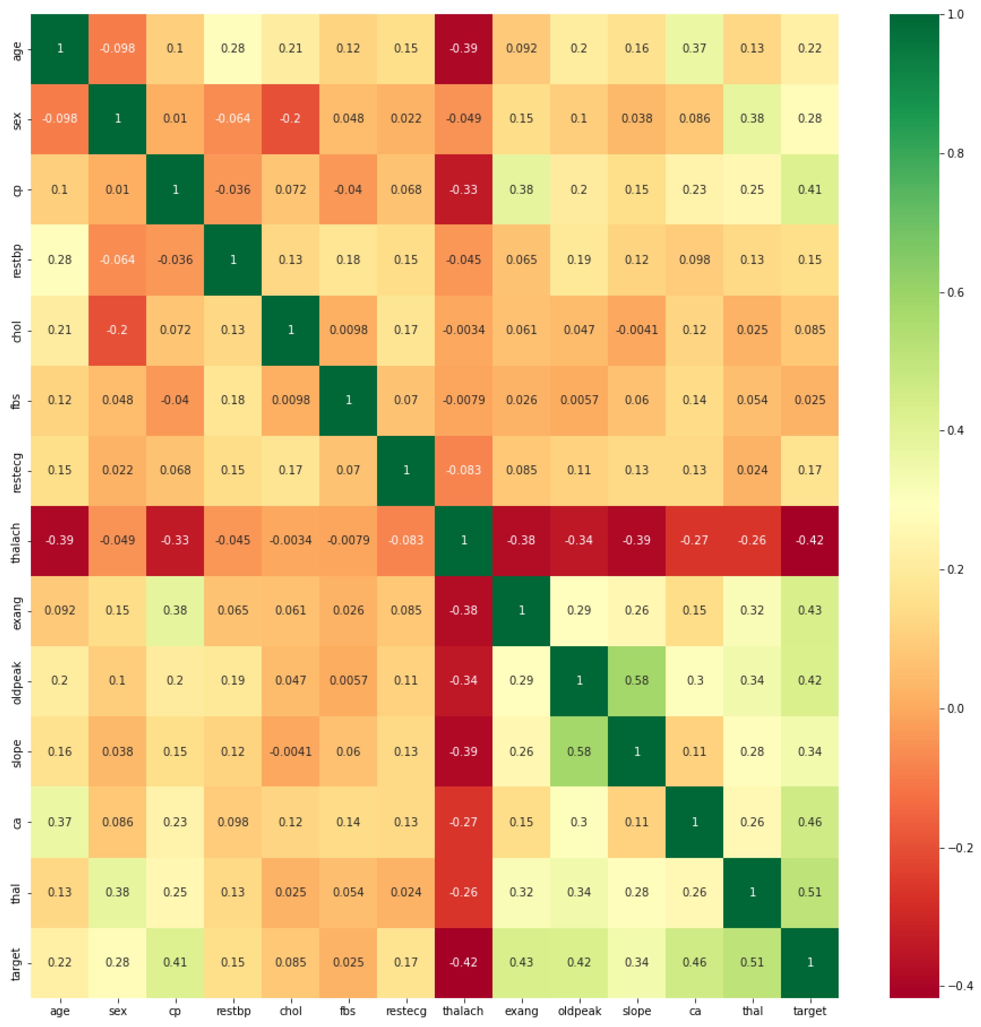
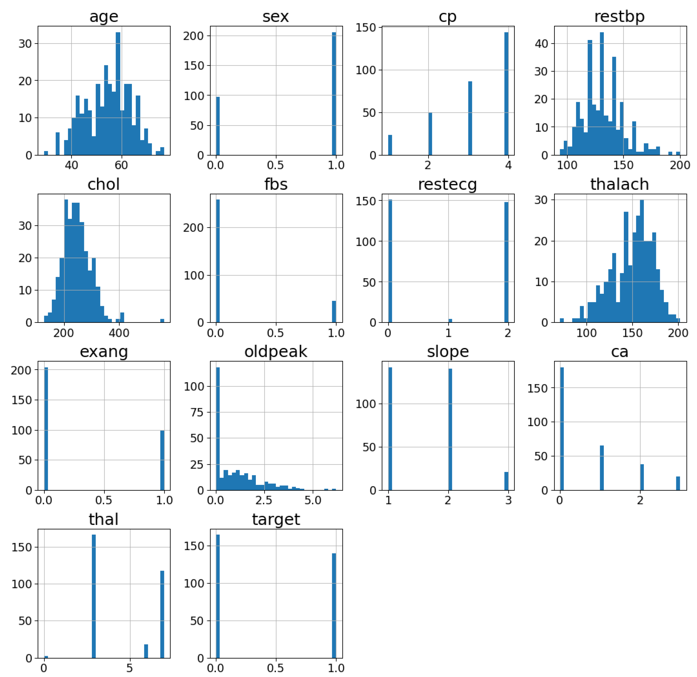
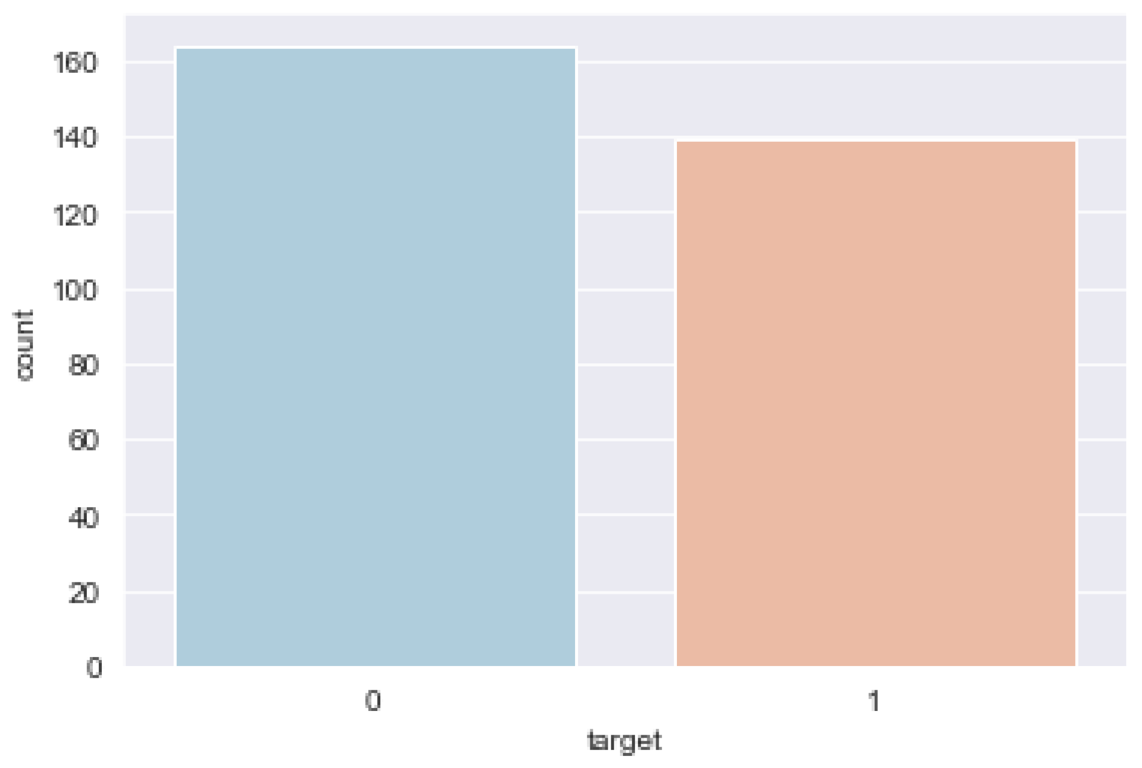
2.1.1. Exploratory Data Analysis
2.1.2. Data Preprocessing
- 1.
- Identifying and handling missing/null valuesIt is critical to correctly identify and handle missing values in data preprocessing; otherwise, we may draw incorrect and erroneous conclusions and inferences from our data. It was observed that there are 6 rows out of the 303 rows containing null values, with four belonging to the variable ‘ca’ and two belonging to the variable ‘thal’. There are two ways to deal with null values: drop or impute. The former is not completely efficient, and it is recommended that we use it only when the dataset has sufficient samples, and we must ensure that there is no additional bias after deleting the data. As a result, we applied the latter and imputed the mean in place of the null values because the null values are few. In this case, we compute the mean of a specific feature, such as ca, that contains a missing value and replace the result for the missing value with the mean. This method can add variance to the dataset and efficiently negate any data loss. Hence, it provides more accurate results than the first method (drop).
- 2.
- Categorical data encodingCategorical data is information that is divided into distinct categories within a dataset. There are some categorical variables in the heart disease dataset: ‘sex’, ‘cp’, ‘fbs’, ‘restecg’, ‘exang’, ‘slope’, ‘ca’ and ‘thal’. Mathematical equations serve as the foundation for ML models. As a result, we can intuitively understand that keeping categorical data in the equation will cause problems because the equations only involve numeric values. For this reason, we converted them to numerical values.
- 3.
- Splitting the dataset into training and testing setsThis step in data preprocessing involves taking the dataset and dividing it into two separate sets. The training dataset is the first subset, which is used to fit or train the model. The second subset, which is referred to as the test dataset, is used is to validate the fit model. In general, we divide the data set into a 70:30 or 80:20 ratio, which means that 70% or 80% of the data is used to train or fit the ML model, and 30% or 20% is used to test or evaluate the trained ML model [37]. However, depending on the shape and size of the data set, the splitting ratio can be changed.
- 4.
- Feature scalingIn data preprocessing, feature scaling is a method for standardizing the independent variables of a dataset within a specific range. To put it another way, feature scaling narrows the range of the independent variables so that we can compare them on common grounds. In the heart disease dataset, we have the variables ‘age’, ‘restbp’, ‘chol’, ‘thalach’, ‘oldpeak’ that do not have the same scale. In such a case, if we compute any two values from the ‘restbp’ and ‘chol’ columns, the ‘chol’ values will dominate the ‘restbp’ values and produce incorrect results. Therefore, we must perform feature scaling in order to eliminate this issue. This is critical for ML algorithms, such as logistic regression, MLP neural networks, and others that use gradient descent as an optimization technique that necessitates data scaling. Furthermore, distance algorithms, such as SVM and KNN, are most influenced by the range of the features. This is due to the fact that they use distances between data points to determine their similarity behind the scenes. The two most-discussed methods to perform feature scaling are Normalization and Standardization.
- NormalizationNormalization is a scaling technique that shifts and rescales values so that they end up ranging between 0 and 1. Min–Max scaling is another name for it. The Normalization equation is written mathematically asHere, and are the minimum and the maximum values of the feature, respectively.
- StandardizationStandardization is a scaling technique in which values are centered around the mean with a unit standard deviation. This means that the features will be rescaled to ensure the mean and the standard deviation are 0 and 1, respectively. For our work, we used the standardization method. The standardization equation is as follows:Here, is the mean of the feature values, and is the standard deviation of the feature values.
2.2. Methodology of the Proposed System
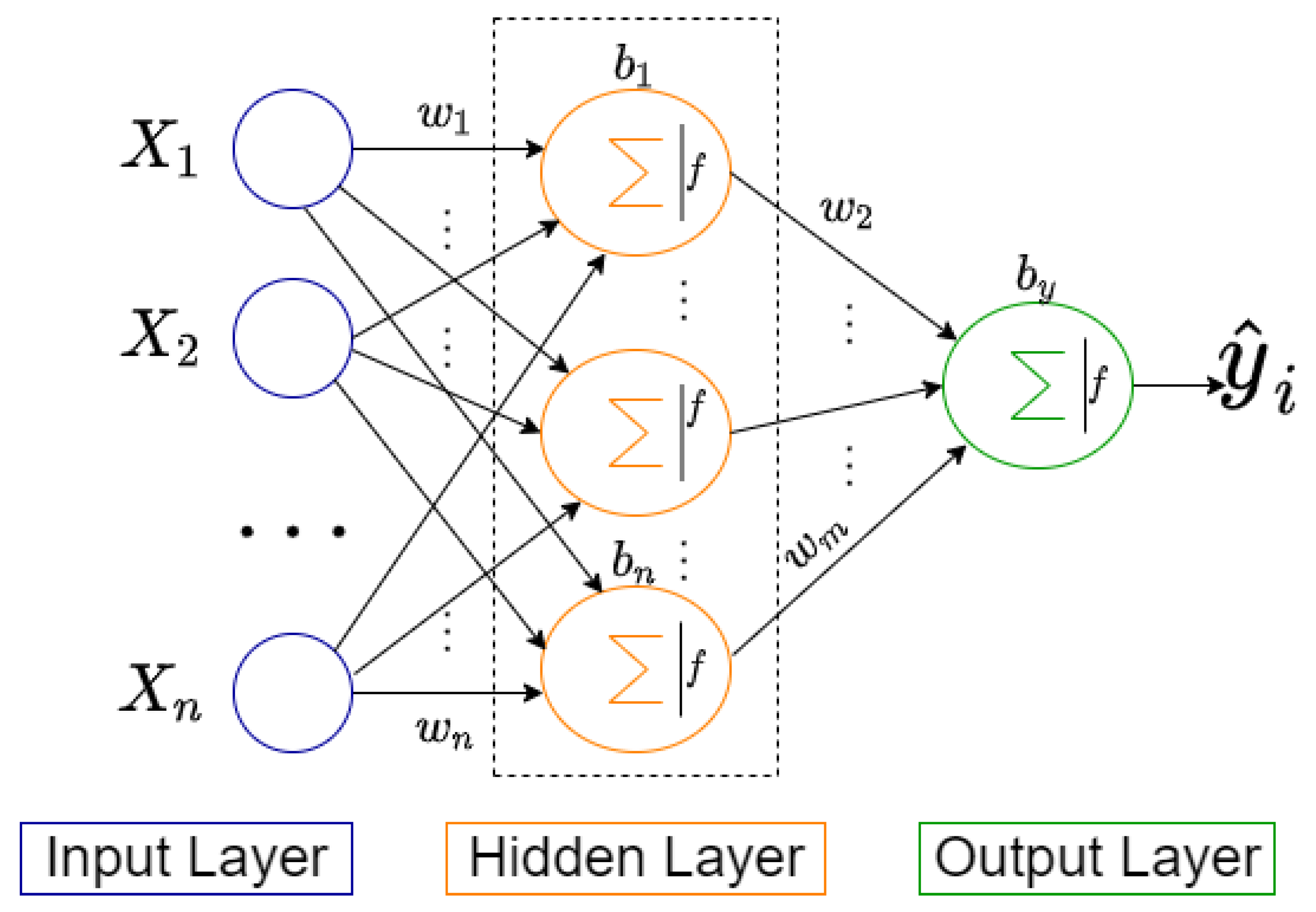
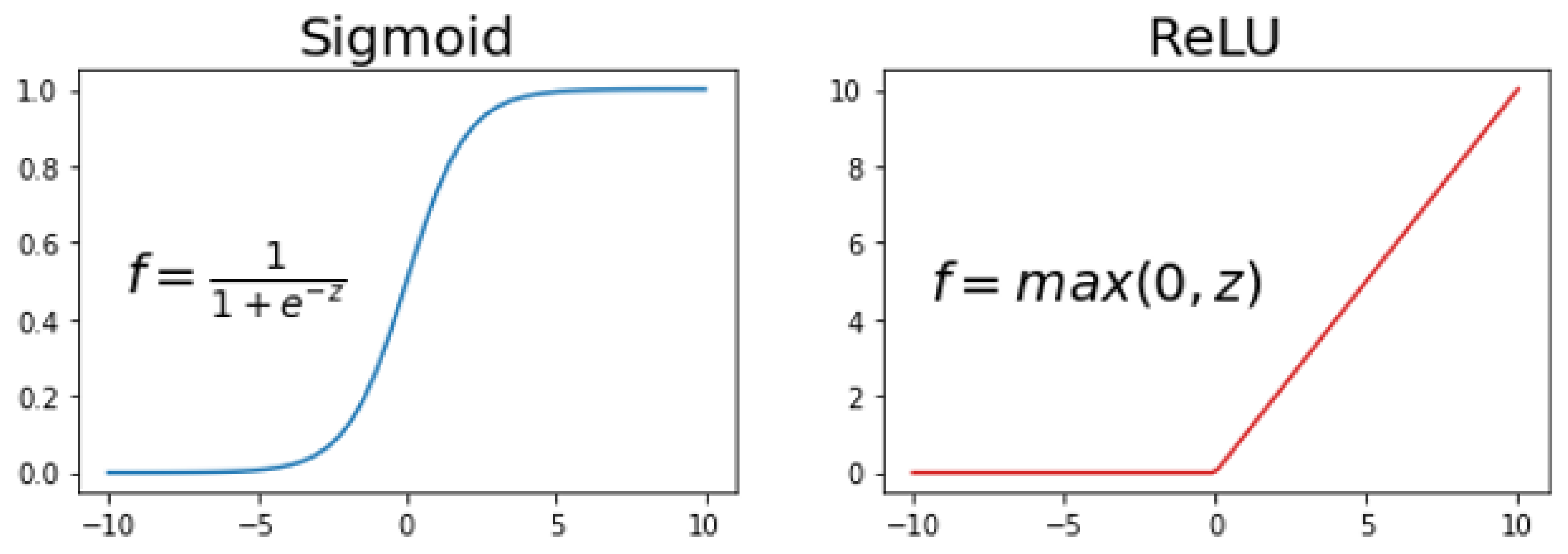
2.2.1. MLP
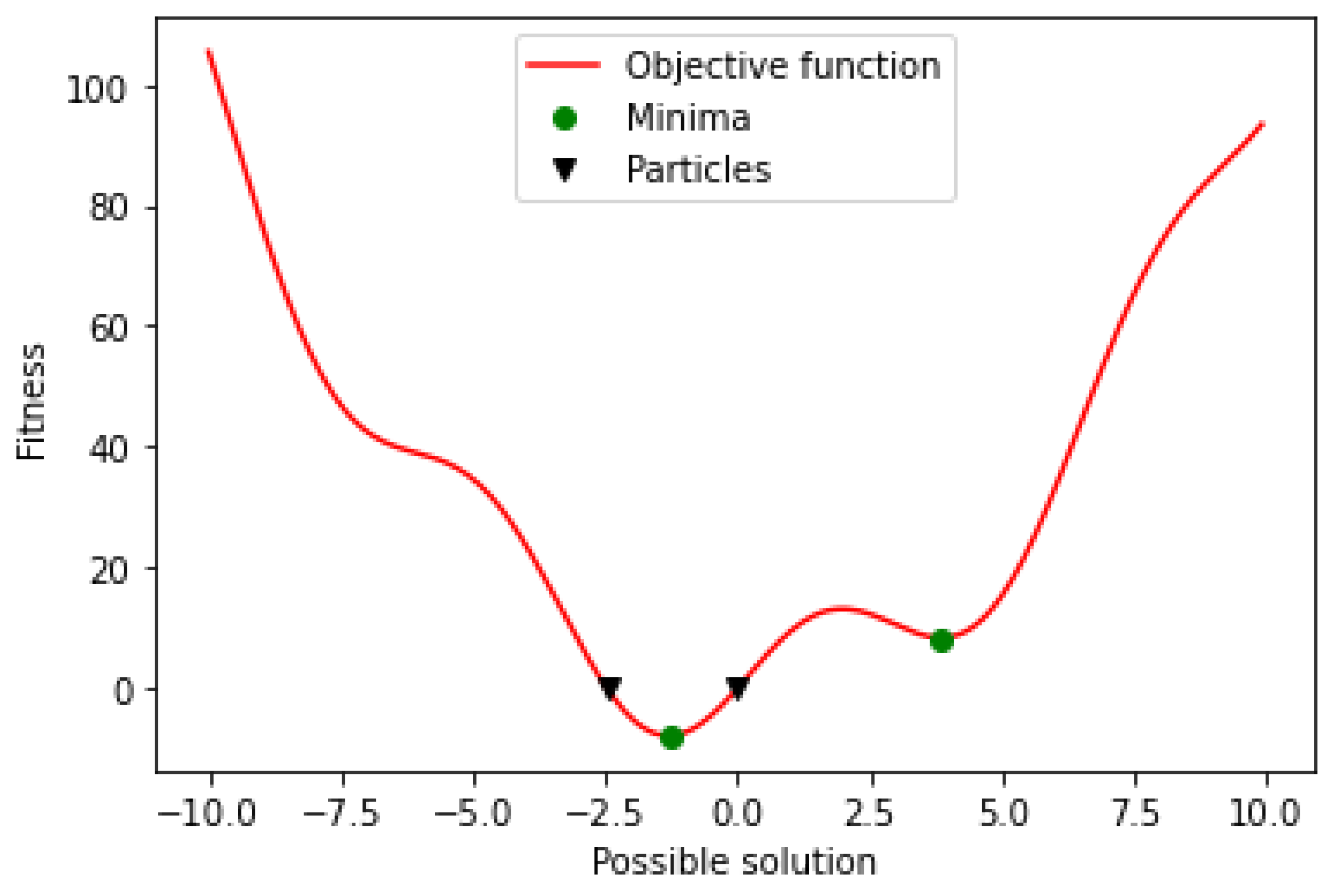
2.2.2. PSO
| Algorithm 1: Pseudocode for the PSO algorithm [53]. |
Input: Output: Population ← ∅; ← ∅; for to do |

|
return |
- 1.
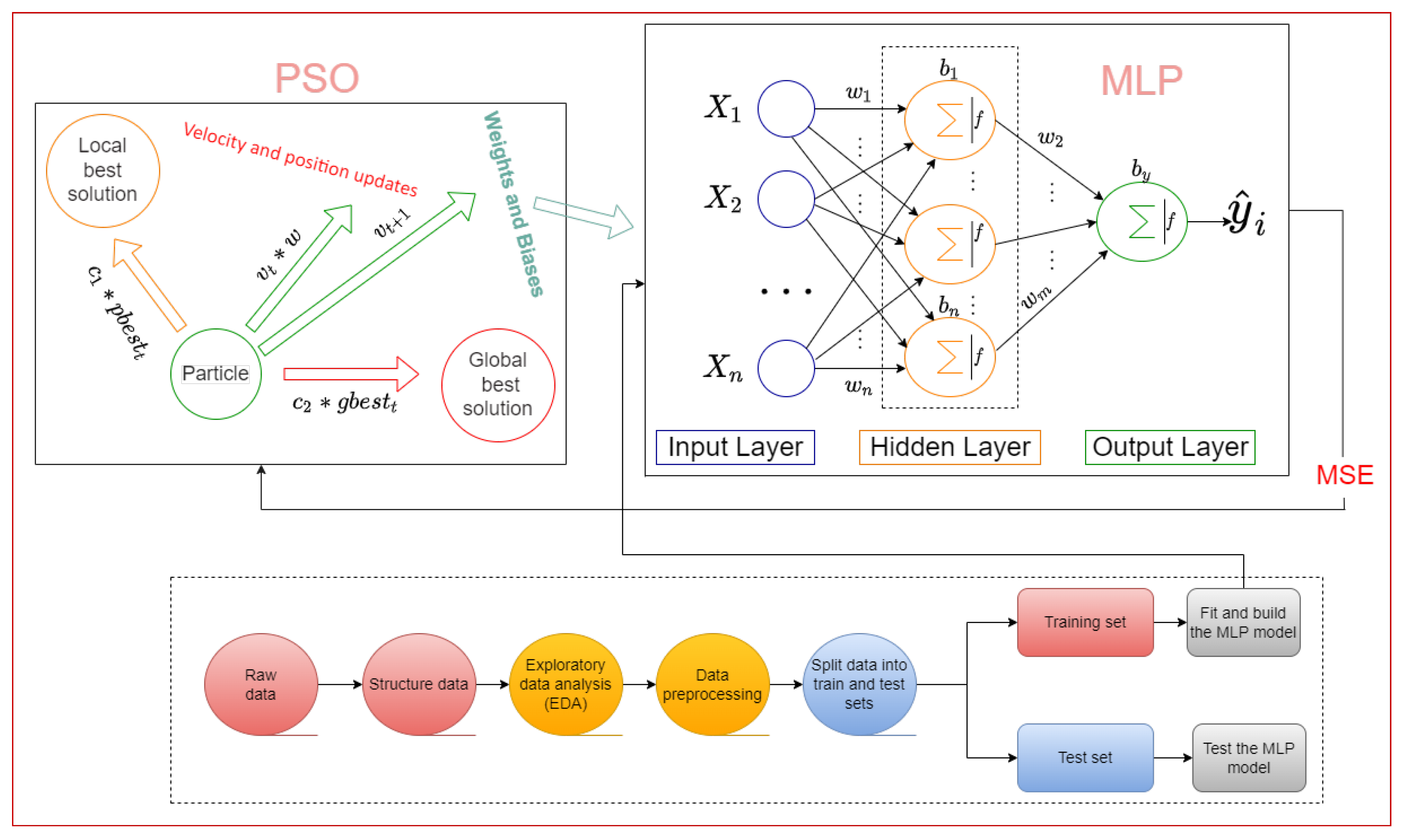
- Evaluate the fitness of each particle or candidate solution in the population using the objective function being optimized.
- 2.
- Update the best individual and global fitnesses and positions by comparing the newly evaluated fitnesses with the prior best individual and global fitnesses and replacing the best fitnesses and positions as needed.
- 3.
- Update the velocity and position of every particle in the population. This updating step is responsible for the optimization ability of the PSO algorithm.
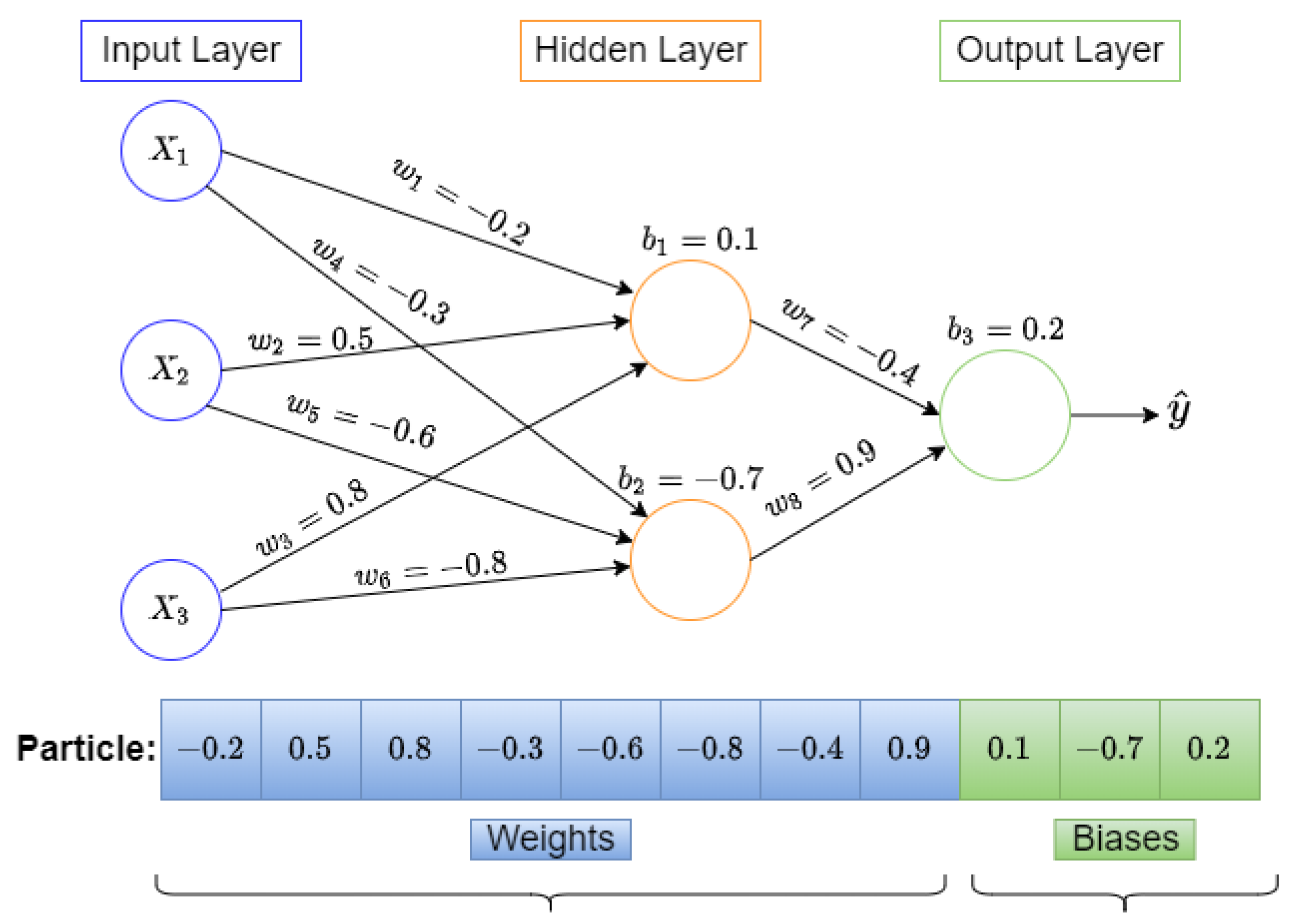
2.2.3. Training MLP Using PSO
2.3. Supervised Machine Learning Algorithms
2.3.1. Logistic Regression
2.3.2. Support Vector Machine
2.3.3. KNN (K-Nearest Neighbors)
2.3.4. Decision Tree
2.3.5. Random Forest
2.3.6. Extra Trees Classifier
2.3.7. Gradient Boosting
2.3.8. Naive Bayes
2.3.9. XGB
3. Experiments and Results
3.1. Experimental Setup
3.2. Performance Evaluation Metrics
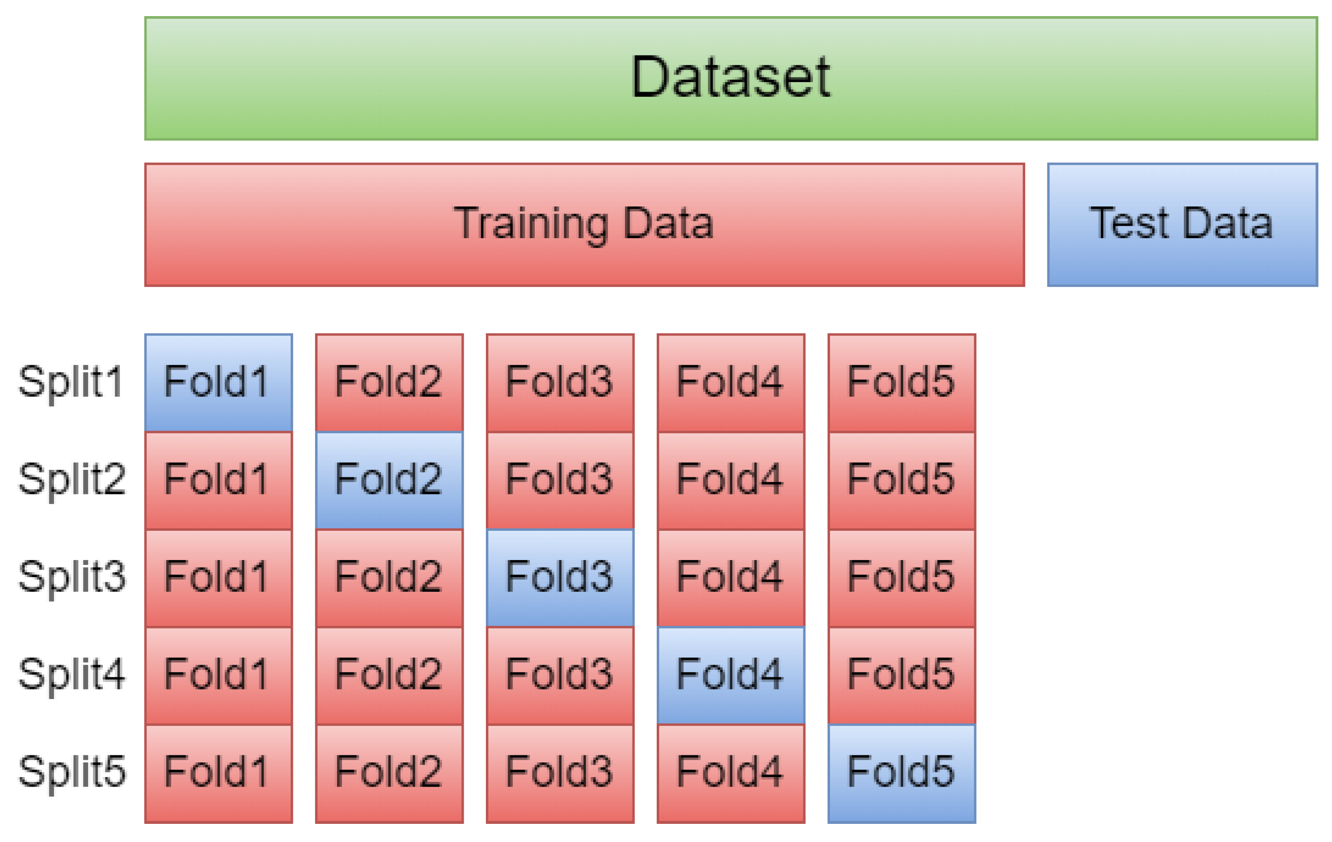
- Randomly shuffle the data.
- Data are split into five groups.
- For each group:
- -
- The model is trained using four of the folds as training data.
- -
- The resulting model is tested on the remaining test data to estimate the performance.

- TP: the number of positive instances in which the model correctly predicts the presence of heart disease.
- TN: the number of negative instances in which the model correctly predicts the absence of heart disease.
- FP: the number of negative instances in which the model incorrectly predicts the presence of heart disease.
- FN: the number of positive instances in which the model incorrectly predicts the absence of heart disease.
- Accuracy: the ratio of correctly predicted instances to all instances, which is defined as follows:
- Precision: the ratio of correctly predicted positive instances to the total number of predicted positive instances, which is defined as follows:
- Recall: the ratio of correctly predicted positive instances to all instances in the actual class (presence), which is defined as follows:
- F1 score: the weighted average of Precision and Recall, which is defined as follows:
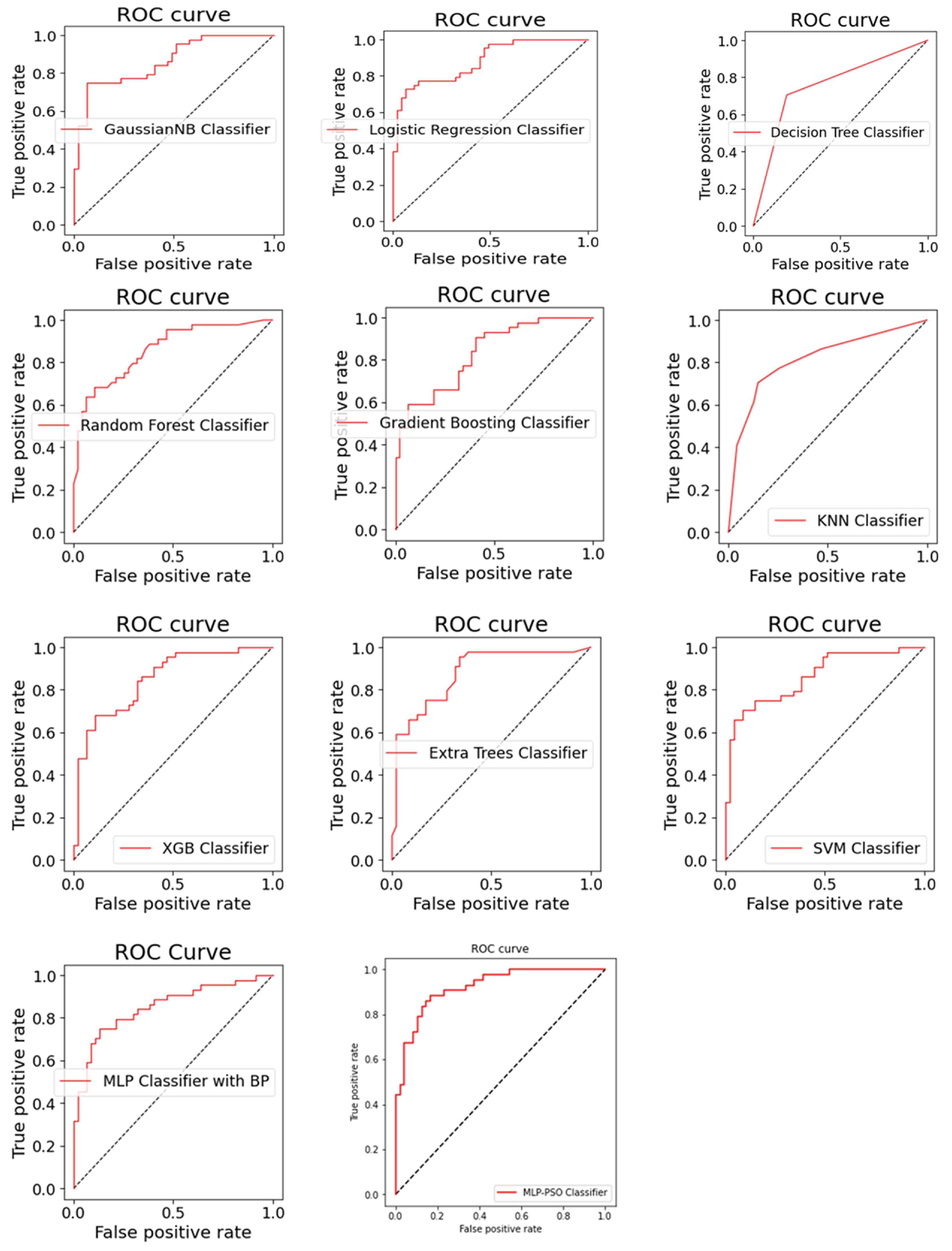
- AUC-ROC Curve: ROC is a probability curve, and AUC represents the measure of a model to distinguish between classes. It tells how much the model is capable of distinguishing between classes. The higher the AUC, the better the model is at distinguishing between the classes. The ROC curve is plotted with the TPR on the y-axis against the FPR on the x-axis. The TPR is a synonym for recall, and FPR is defined as as follows:
3.3. Results and Discussion
4. Conclusions and Future Directions
Author Contributions
Funding
Institutional Review Board Statement
Informed Consent Statement
Data Availability Statement
Conflicts of Interest
Appendix A. MLP Training Problem Representation Using PSO

Appendix B. Model Hyperparameters

| Algorithm | Parameters | Algorithm | Parameters |
|---|---|---|---|
| Decision Tree Classifier | criterion = ‘Gini’ min_samples_leaf = 1 min_samples_split = 2 max_features = log2(n_features) splitter = ‘best’ | Logistic Regression Classifier | C = 1.5 fit_intercpet = ‘True’ Penalty = ‘12’ |
| Extra Trees Classifier | Criterion = ‘Gini’ min_samples_leaf = 1 min_samples_split = 2 max_features = log2(n_features) n_estimators = 100 | MLP Classifier with BP | hidden_layer_size = 30 activation = ‘relu’ learning_rate = ‘adaptive’ momentum = 0.9 optimizer = ‘adam’ |
| GaussianNB Classifier | var_smoothing = 1 priors = ‘None’ | Random Forest Classifier | max_features = sqrt (n_features) n_estimators = 1000 criterion = ‘Gini’ |
| Gradient Boosting Classifier | criterion = ‘friedman_mse’ loss = ‘deviance’ learning_rate = 0.1 n_estimators = 100 max_depth = 3 max_features = log2(n_features) | SVM Classifier | C = 1 coef0 = 10 degree = 3 gamma = 0.1 kernel = ‘rbf’ |
| KNN Classifier | metric = ‘minkowski’ n_neighbors = 5 p = 2 weights = ‘uniform’ | XGB Classifier | colsample_bytree = 0.6 reg_lambda = 0.68 reg_alpha = 72 max_depth = 15 min_child_weight = 1 gamma = 3.27 n_estimators = 300 |
Appendix C. ROC Curves

Appendix D. Source Code
References
- Richens, J.G.; Lee, C.M.; Johri, S. Improving the accuracy of medical diagnosis with causal machine learning. Nat. Commun. 2020, 11, 3923. [Google Scholar] [CrossRef] [PubMed]
- Al Bataineh, A.; Jarrah, A. High Performance Implementation of Neural Networks Learning Using Swarm Optimization Algorithms for EEG Classification Based on Brain Wave Data. Int. J. Appl. Metaheuristic Comput. 2022, 13, 1–17. [Google Scholar] [CrossRef]
- Samieinasab, M.; Torabzadeh, S.A.; Behnam, A.; Aghsami, A.; Jolai, F. Meta-Health Stack: A new approach for breast cancer prediction. Healthc. Anal. 2022, 2, 100010. [Google Scholar] [CrossRef]
- Hameed, B.Z.; Prerepa, G.; Patil, V.; Shekhar, P.; Zahid Raza, S.; Karimi, H.; Paul, R.; Naik, N.; Modi, S.; Vigneswaran, G.; et al. Engineering and clinical use of artificial intelligence (AI) with machine learning and data science advancements: Radiology leading the way for future. Ther. Adv. Urol. 2021, 13, 17562872211044880. [Google Scholar] [CrossRef] [PubMed]
- Committee on Diagnostic Error in Health Care; Board on Health Care Services; Institute of Medicine; The National Academies of Sciences, Engineering, and Medicine. Improving Diagnosis in Health Care; Balogh, E., Miller, B., Ball, J., Eds.; National Academies Press: Washington, DC, USA, 2015.
- Sinsky, C.; Colligan, L.; Li, L.; Prgomet, M.; Reynolds, S.; Goeders, L.; Westbrook, J.; Tutty, M.; Blike, G. Allocation of physician time in ambulatory practice: A time and motion study in 4 specialties. Ann. Intern. Med. 2016, 165, 753–760. [Google Scholar] [CrossRef] [PubMed]
- Yoo, I.; Alafaireet, P.; Marinov, M.; Pena-Hernandez, K.; Gopidi, R.; Chang, J.F.; Hua, L. Data mining in healthcare and biomedicine: A survey of the literature. J. Med. Syst. 2012, 36, 2431–2448. [Google Scholar] [CrossRef] [PubMed]
- Oikonomou, E.K.; Williams, M.C.; Kotanidis, C.P.; Desai, M.Y.; Marwan, M.; Antonopoulos, A.S.; Thomas, K.E.; Thomas, S.; Akoumianakis, I.; Fan, L.M.; et al. A novel machine learning-derived radiotranscriptomic signature of perivascular fat improves cardiac risk prediction using coronary CT angiography. Eur. Heart J. 2019, 40, 3529–3543. [Google Scholar] [CrossRef] [PubMed]
- Warnat-Herresthal, S.; Perrakis, K.; Taschler, B.; Becker, M.; Baßler, K.; Beyer, M.; Günther, P.; Schulte-Schrepping, J.; Seep, L.; Klee, K.; et al. Scalable prediction of acute myeloid leukemia using high-dimensional machine learning and blood transcriptomics. Iscience 2020, 23, 100780. [Google Scholar] [CrossRef] [Green Version]
- Tsao, C.W.; Aday, A.W.; Almarzooq, Z.I.; Alonso, A.; Beaton, A.Z.; Bittencourt, M.S.; Boehme, A.K.; Buxton, A.E.; Carson, A.P.; Commodore-Mensah, Y.; et al. Heart Disease and Stroke Statistics—2022 Update: A Report From the American Heart Association. Circulation 2022, 145, e153–e639. [Google Scholar] [CrossRef] [PubMed]
- Petersen, K.S.; Kris-Etherton, P.M. Diet Quality Assessment and the Relationship between Diet Quality and Cardiovascular Disease Risk. Nutrients 2021, 13, 4305. [Google Scholar] [CrossRef]
- Abubakar, I.; Tillmann, T.; Banerjee, A. Global, regional, and national age-sex specific all-cause and cause-specific mortality for 240 causes of death, 1990–2013: A systematic analysis for the Global Burden of Disease Study 2013. Lancet 2015, 385, 117–171. [Google Scholar]
- Mendis, S.; Puska, P.; Norrving, B.E.; World Health Organization. Global Atlas on Cardiovascular Disease Prevention and Control; World Health Organization: Geneva, Switzerland, 2011. [Google Scholar]
- Urbich, M.; Globe, G.; Pantiri, K.; Heisen, M.; Bennison, C.; Wirtz, H.S.; Di Tanna, G.L. A systematic review of medical costs associated with heart failure in the USA (2014–2020). Pharmacoeconomics 2020, 38, 1219–1236. [Google Scholar] [CrossRef] [PubMed]
- Vamsi, B.; Doppala, B.P.; Thirupathi Rao, N.; Bhattacharyya, D. Comparative Analysis of Prevalent Disease by Preprocessing Techniques Using Big Data and Machine Learning: An Extensive Review. In Machine Intelligence and Soft Computing; Springer: Berlin/Heidelberg, Germany, 2021; pp. 27–38. [Google Scholar]
- Kumar, Y.; Koul, A.; Singla, R.; Ijaz, M.F. Artificial intelligence in disease diagnosis: A systematic literature review, synthesizing framework and future research agenda. J. Ambient. Intell. Humaniz. Comput. 2022, 1–28. [Google Scholar] [CrossRef] [PubMed]
- Al Bataineh, A. A comparative analysis of nonlinear machine learning algorithms for breast cancer detection. Int. J. Mach. Learn. Comput. 2019, 9, 248–254. [Google Scholar] [CrossRef]
- Doppala, B.P.; Bhattacharyya, D. A Novel Approach to Predict Cardiovascular Diseases Using Machine Learning. In Machine Intelligence and Soft Computing; Springer: Berlin/Heidelberg, Germany, 2021; pp. 71–80. [Google Scholar]
- Doppala, B.P.; Bhattacharyya, D.; Chakkravarthy, M.; Kim, T.H. A hybrid machine learning approach to identify coronary diseases using feature selection mechanism on heart disease dataset. Distrib. Parallel Databases 2021, 1–20. [Google Scholar] [CrossRef]
- Mallesh, N.; Zhao, M.; Meintker, L.; Höllein, A.; Elsner, F.; Lüling, H.; Haferlach, T.; Kern, W.; Westermann, J.; Brossart, P.; et al. Knowledge transfer to enhance the performance of deep learning models for automated classification of B cell neoplasms. Patterns 2021, 2, 100351. [Google Scholar] [CrossRef] [PubMed]
- Muibideen, M.; Prasad, R. A Fast Algorithm for Heart Disease Prediction using Bayesian Network Model. arXiv 2020, arXiv:2012.09429. [Google Scholar]
- Khateeb, N.; Usman, M. Efficient heart disease prediction system using K-nearest neighbor classification technique. In Proceedings of the International Conference on Big Data and Internet of Thing, London, UK, 20–22 December 2017; pp. 21–26. [Google Scholar]
- Chang, V.; Bhavani, V.R.; Xu, A.Q.; Hossain, M. An artificial intelligence model for heart disease detection using machine learning algorithms. Healthc. Anal. 2022, 2, 100016. [Google Scholar] [CrossRef]
- Bharti, R.; Khamparia, A.; Shabaz, M.; Dhiman, G.; Pande, S.; Singh, P. Prediction of heart disease using a combination of machine learning and deep learning. Comput. Intell. Neurosci. 2021, 2021, 8387680. [Google Scholar] [CrossRef] [PubMed]
- Muhammad, Y.; Tahir, M.; Hayat, M.; Chong, K.T. Early and accurate detection and diagnosis of heart disease using intelligent computational model. Sci. Rep. 2020, 10, 19747. [Google Scholar] [CrossRef] [PubMed]
- Gudadhe, M.; Wankhade, K.; Dongre, S. Decision support system for heart disease based on support vector machine and artificial neural network. In Proceedings of the 2010 International Conference on Computer and Communication Technology (ICCCT), Allahabad, India, 17–19 September 2010; pp. 741–745. [Google Scholar]
- Ali, L.; Niamat, A.; Khan, J.A.; Golilarz, N.A.; Xingzhong, X.; Noor, A.; Nour, R.; Bukhari, S.A.C. An optimized stacked support vector machines based expert system for the effective prediction of heart failure. IEEE Access 2019, 7, 54007–54014. [Google Scholar] [CrossRef]
- Jalali, S.M.J.; Karimi, M.; Khosravi, A.; Nahavandi, S. An efficient neuroevolution approach for heart disease detection. In Proceedings of the 2019 IEEE International Conference on Systems, Man and Cybernetics (SMC 2019), Bari, Italy, 6–9 October 2019; pp. 3771–3776. [Google Scholar]
- Bhatia, S.; Prakash, P.; Pillai, G. SVM based decision support system for heart disease classification with integer-coded genetic algorithm to select critical features. In Proceedings of the World Congress on Engineering and Computer Science, San Francisco, CA, USA, 22–24 October 2008; pp. 34–38. [Google Scholar]
- Polat, K.; Güneş, S. A hybrid approach to medical decision support systems: Combining feature selection, fuzzy weighted pre-processing and AIRS. Comput. Methods Programs Biomed. 2007, 88, 164–174. [Google Scholar] [CrossRef] [PubMed]
- Zhang, C.; Shao, H.; Li, Y. Particle swarm optimisation for evolving artificial neural network. In Proceedings of the 2000 IEEE International Conference on Systems, Man and Cyberbetics—“Cyberbetics Evolving to Systems, Humans, Organizations, and their Complex Interactions” (SMC 2000), Nashville, TN, USA, 8–11 October 2000; Volume 4, pp. 2487–2490. [Google Scholar]
- Hamed, H.N.A.; Shamsuddin, S.M.; Salim, N. Particle swarm optimization for neural network learning enhancement. J. Teknol. 2008, 49, 13–26. [Google Scholar]
- Beheshti, Z.; Shamsuddin, S.M. Improvement of Multi-Layer Perceptron (MLP) training using optimization algorithms. Technology 2010, 27, 28. [Google Scholar]
- Lee, K.Y.; Park, J.B. Application of particle swarm optimization to economic dispatch problem: Advantages and disadvantages. In Proceedings of the 2006 IEEE PES Power Systems Conference and Exposition, Atlanta, GA, USA, 29 October–1 November 2006; pp. 188–192. [Google Scholar]
- Gad, A.G. Particle Swarm Optimization Algorithm and Its Applications: A Systematic Review. Arch. Comput. Methods Eng. 2022, 29, 2531–2561. [Google Scholar] [CrossRef]
- Janosi, A.; Steinbrunn, W.; Pfisterer, M.; Detrano, R. Heart Disease Data Set. The UCI KDD Archive. 1988. Available online: https://archive.ics.uci.edu/ml/datasets/heart+disease (accessed on 22 June 2022).
- Brownlee, J. Machine Learning Mastery with Python: Understand Your Data, Create Accurate Models, and Work Projects End-to-End; Machine Learning Mastery: San Juan, PR, USA, 2016. [Google Scholar]
- Brownlee, J. Deep Learning with Python: Develop Deep Learning Models on Theano and TensorFlow using Keras; Machine Learning Mastery: San Juan, PR, USA, 2016. [Google Scholar]
- Al Bataineh, A.; Kaur, D. A comparative study of different curve fitting algorithms in artificial neural network using housing dataset. In Proceedings of the IEEE National Aerospace and Electronics Conference (NAECON 2018), Dayton, OH, USA, 23–26 July 2018; pp. 174–178. [Google Scholar]
- Mosteller, F.; Tukey, J.W. Data analysis, including statistics. In Handbook of Social Psychology; Addison-Wesley: Boston, MA, USA, 1968; Volume 2, pp. 80–203. [Google Scholar]
- Bataineh, A.S.A. A gradient boosting regression based approach for energy consumption prediction in buildings. Adv. Energy Res. 2019, 6, 91–101. [Google Scholar]
- LeCun, Y.; Bengio, Y.; Hinton, G. Deep learning. Nature 2015, 521, 436–444. [Google Scholar] [CrossRef]
- Al Bataineh, A.; Mairaj, A.; Kaur, D. Autoencoder based semi-supervised anomaly detection in turbofan engines. Int. J. Adv. Comput. Sci. Appl. 2020, 11, 41–47. [Google Scholar] [CrossRef]
- Rumelhart, D.E.; Hinton, G.E.; Williams, R.J. Learning Internal Representations by Error Propagation; Technical Report; Institute for Cognitive Science, University of California: San Diego, CA, USA, 1985. [Google Scholar]
- Al Bataineh, A.; Kaur, D. Optimal convolutional neural network architecture design using clonal selection algorithm. Int. J. Mach. Learn. Comput. 2019, 9, 788–794. [Google Scholar] [CrossRef]
- Al Bataineh, A.; Kaur, D. Immunocomputing-Based Approach for Optimizing the Topologies of LSTM Networks. IEEE Access 2021, 9, 78993–79004. [Google Scholar] [CrossRef]
- Hofmeyr, S.A.; Forrest, S. Architecture for an artificial immune system. Evol. Comput. 2000, 8, 443–473. [Google Scholar] [CrossRef] [PubMed]
- Bäck, T.; Fogel, D.B.; Michalewicz, Z. Handbook of evolutionary computation. Release 1997, 97, B1. [Google Scholar]
- Kennedy, J. Swarm intelligence. In Handbook of Nature-Inspired and Innovative Computing; Springer: Berlin/Heidelberg, Germany, 2006; pp. 187–219. [Google Scholar]
- Eberhart, R.; Kennedy, J. A new optimizer using particle swarm theory. In Proceedings of the Sixth International Symposium on Micro Machine and Human Science, Nagoya, Japan, 4–6 October 1995; pp. 39–43. [Google Scholar]
- Eberhart, R.C.; Shi, Y.; Kennedy, J. Swarm Intelligence; Elsevier: Amsterdam, The Netherlands, 2001. [Google Scholar]
- Blondin, J. Particle Swarm Optimization: A Tutorial. 2009. Available online: http://http://cs.armstrong.edu/saad/csci8100/pso_tutorial.pdf (accessed on 22 June 2022).
- Brownlee, J. Clever Algorithms: Nature-Inspired Programming Recipes; Lulu Press, Inc.: Research Triangle, NC, USA, 2011. [Google Scholar]
- Van Den Bergh, F. An Analysis of Particle Swarm Optimizers (PSO); University of Pretoria: Pretoria, South Africa, 2001; pp. 78–85. [Google Scholar]
- Hosmer, D.W., Jr.; Lemeshow, S.; Sturdivant, R.X. Applied Logistic Regression; John Wiley & Sons: Hoboken, NJ, USA, 2013; Volume 398. [Google Scholar]
- Cortes, C.; Vapnik, V. Support vector machine. Mach. Learn. 1995, 20, 273–297. [Google Scholar] [CrossRef]
- Cover, T.; Hart, P. Nearest neighbor pattern classification. IEEE Trans. Inf. Theory 1967, 13, 21–27. [Google Scholar] [CrossRef] [Green Version]
- Danielsson, P.E. Euclidean distance mapping. Comput. Graph. Image Process. 1980, 14, 227–248. [Google Scholar] [CrossRef] [Green Version]
- Quinlan, J.R. Probabilistic decision trees. In Machine Learning; Elsevier: Amsterdam, The Netherlands, 1990; pp. 140–152. [Google Scholar]
- Breiman, L. Random forests. Mach. Learn. 2001, 45, 5–32. [Google Scholar] [CrossRef] [Green Version]
- Geurts, P.; Ernst, D.; Wehenkel, L. Extremely randomized trees. Mach. Learn. 2006, 63, 3–42. [Google Scholar] [CrossRef] [Green Version]
- Friedman, J.H. Stochastic gradient boosting. Comput. Stat. Data Anal. 2002, 38, 367–378. [Google Scholar] [CrossRef]
- Rish, I. An empirical study of the naive Bayes classifier. In Proceedings of the IJCAI 2001 Workshop on Empirical Methods in Artificial Intelligence, Seattle, WA, USA, 4–10 August 2001; Volume 3, pp. 41–46. [Google Scholar]
- Chen, T.; Guestrin, C. Xgboost: A scalable tree boosting system. In Proceedings of the 22nd ACM Sigkdd International Conference on Knowledge Discovery and Data Mining, San Francisco, CA, USA, 13–17 August 2016; pp. 785–794. [Google Scholar]
- Oliphant, T.E. Python for Scientific Computing. Comput. Sci. Eng. 2007, 9, 10–20. [Google Scholar] [CrossRef] [Green Version]
- Pedregosa, F.; Varoquaux, G.; Gramfort, A.; Michel, V.; Thirion, B.; Grisel, O.; Blondel, M.; Prettenhofer, P.; Weiss, R.; Dubourg, V.; et al. Scikit-learn: Machine learning in Python. J. Mach. Learn. Res. 2011, 12, 2825–2830. [Google Scholar]
- McKinney, W. Data structures for statistical computing in python. In Proceedings of the 9th Python in Science Conference, Austin, TX, USA, 28 June–3 July 2010; Volume 445, pp. 51–56. [Google Scholar]
- Oliphant, T.E. A Guide to NumPy; Trelgol Publishing: Spanish Fork, UT, USA, 2006; Volume 1. [Google Scholar]
- Hunter, J.D. Matplotlib: A 2D graphics environment. Comput. Sci. Eng. 2007, 9, 90–95. [Google Scholar] [CrossRef]
- Miranda, L.J. PySwarms: A research toolkit for Particle Swarm Optimization in Python. J. Open Source Softw. 2018, 3, 433. [Google Scholar] [CrossRef] [Green Version]
- Brownlee, J. Statistical Methods for Machine Learning: Discover How to Transform Data into Knowledge with Python; Machine Learning Mastery: San Juan, PR, USA, 2018. [Google Scholar]


| Parameter | Value |
|---|---|
| Swarm size | 100 |
| Iterations | 50 |
| 0.4 | |
| 0.5 | |
| 0.5 | |
| 0.3 | |
| w | 0.9 |
| Algorithm | Accuracy | AUC | Precision | Recall | F1 Score |
|---|---|---|---|---|---|
| MLP-PSO Classifier | 0.846 | 0.848 | 0.808 | 0.883 | 0.844 |
| Decision Tree Classifier | 0.758 | 0.756 | 0.775 | 0.704 | 0.738 |
| Extra Trees Classifier | 0.769 | 0.766 | 0.810 | 0.681 | 0.740 |
| GaussianNB Classifier | 0.824 | 0.821 | 0.868 | 0.750 | 0.804 |
| Gradient Boosting Classifier | 0.714 | 0.712 | 0.725 | 0.659 | 0.690 |
| KNN Classifier | 0.780 | 0.777 | 0.815 | 0.704 | 0.756 |
| Logistic Regression Classifier | 0.813 | 0.808 | 0.909 | 0.681 | 0.779 |
| MLP Classifier with BP | 0.802 | 0.799 | 0.861 | 0.704 | 0.775 |
| Random Forest Classifier | 0.791 | 0.787 | 0.857 | 0.681 | 0.759 |
| SVM Classifier | 0.813 | 0.809 | 0.885 | 0.704 | 0.784 |
| XGB Classifier | 0.769 | 0.766 | 0.810 | 0.681 | 0.740 |
Publisher’s Note: MDPI stays neutral with regard to jurisdictional claims in published maps and institutional affiliations. |
© 2022 by the authors. Licensee MDPI, Basel, Switzerland. This article is an open access article distributed under the terms and conditions of the Creative Commons Attribution (CC BY) license (https://creativecommons.org/licenses/by/4.0/).
Share and Cite
Al Bataineh, A.; Manacek, S. MLP-PSO Hybrid Algorithm for Heart Disease Prediction. J. Pers. Med. 2022, 12, 1208. https://doi.org/10.3390/jpm12081208
Al Bataineh A, Manacek S. MLP-PSO Hybrid Algorithm for Heart Disease Prediction. Journal of Personalized Medicine. 2022; 12(8):1208. https://doi.org/10.3390/jpm12081208
Chicago/Turabian StyleAl Bataineh, Ali, and Sarah Manacek. 2022. "MLP-PSO Hybrid Algorithm for Heart Disease Prediction" Journal of Personalized Medicine 12, no. 8: 1208. https://doi.org/10.3390/jpm12081208