
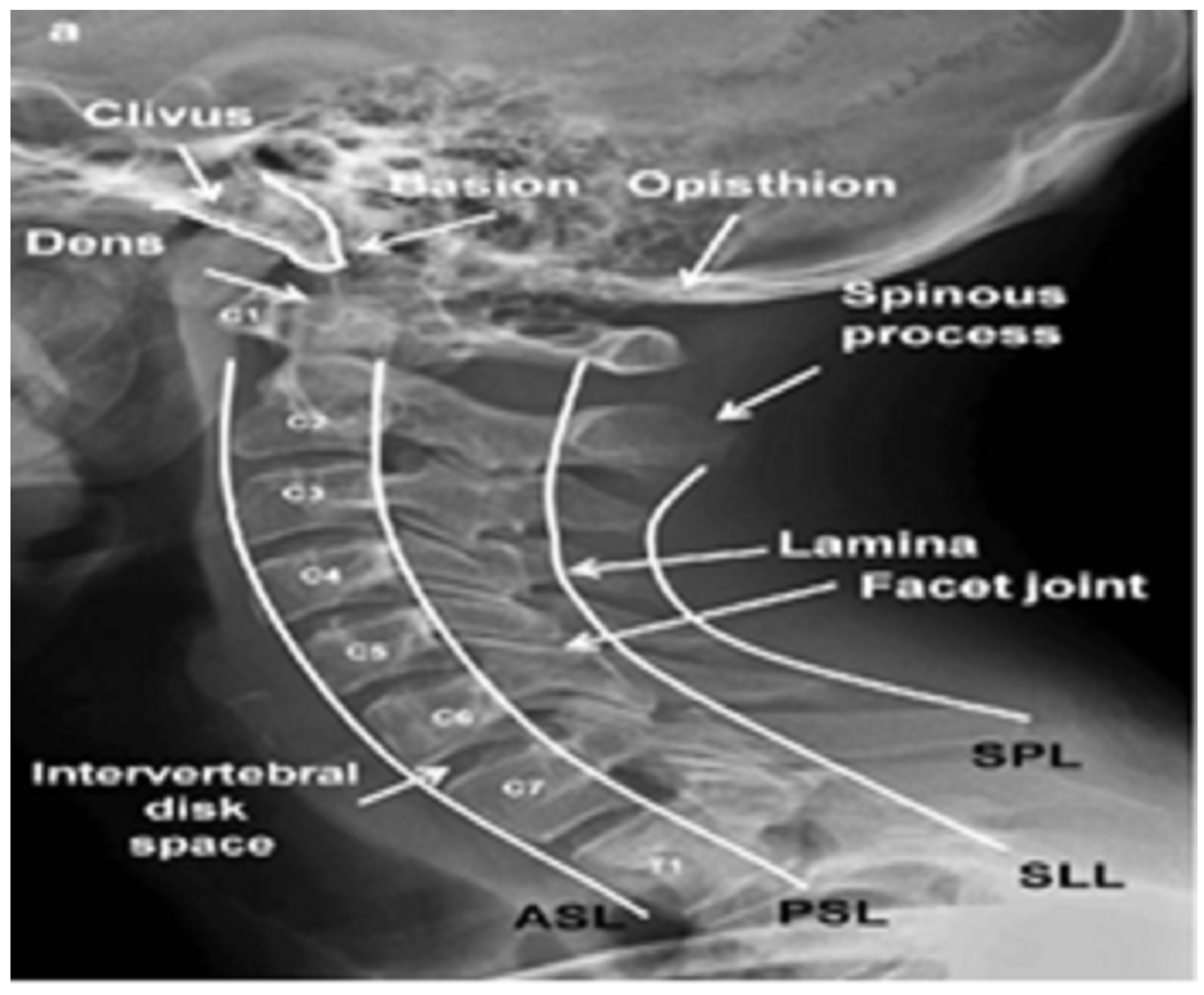
Classification of Cervical Spine Fracture and Dislocation Using Refined Pre-Trained Deep Model and Saliency Map
 , ,
, ,
Abstract
:1. Introduction
- 1.
- Using X-ray images, a new pre-trained CNN-based model for detecting fractures and dislocation in the CS.
- 2.
- The proposed model is efficient, easily installed, and executed using regular configuration PC machines or low-cost embedded systems.
- 3.
- The proposed model successfully classified unlabeled 68 X-ray images of CS.
- 4.
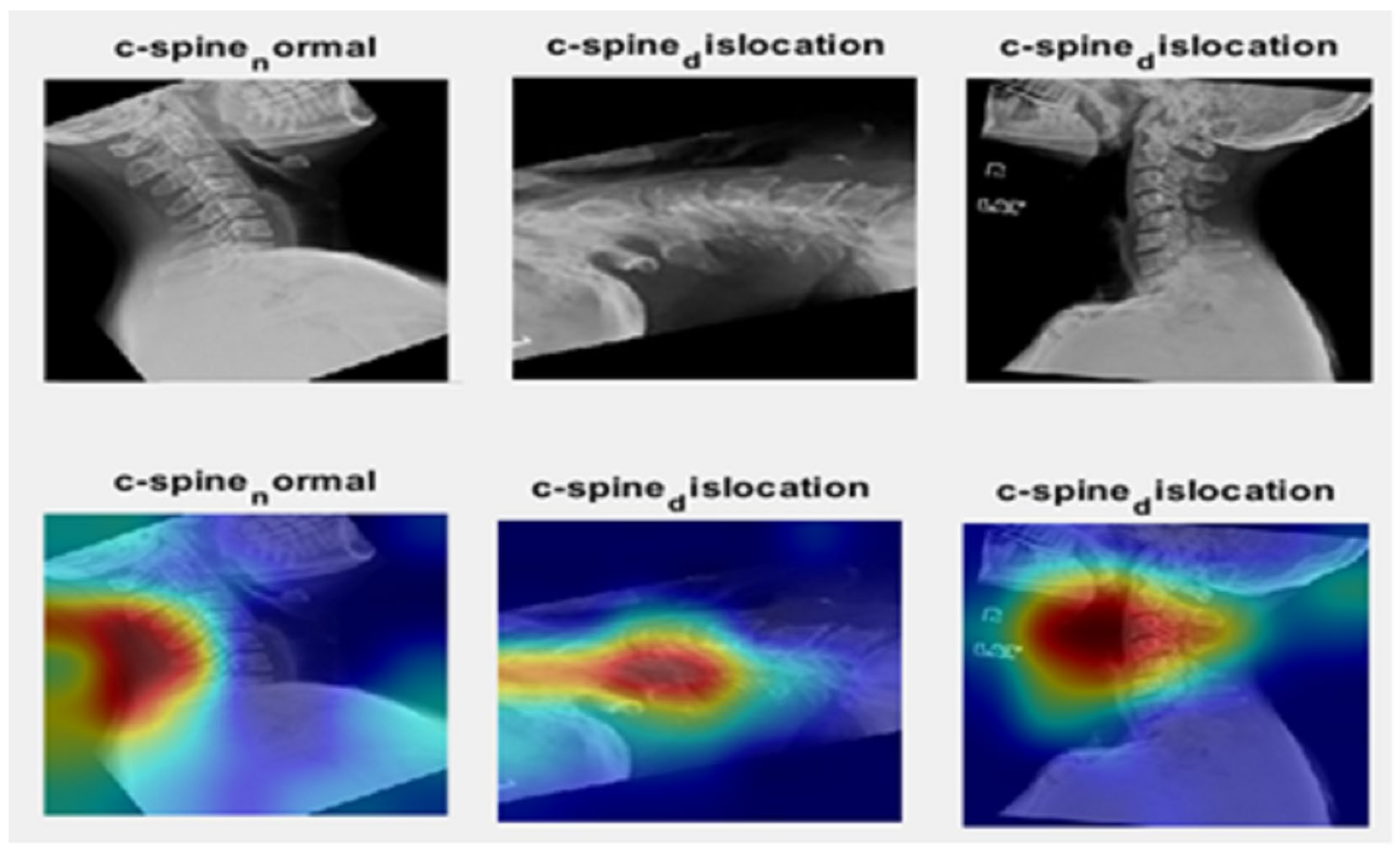
- The ability of the proposed model to successfully detect the cervical spine was proven by the saliency map.
2. Materials and Methods
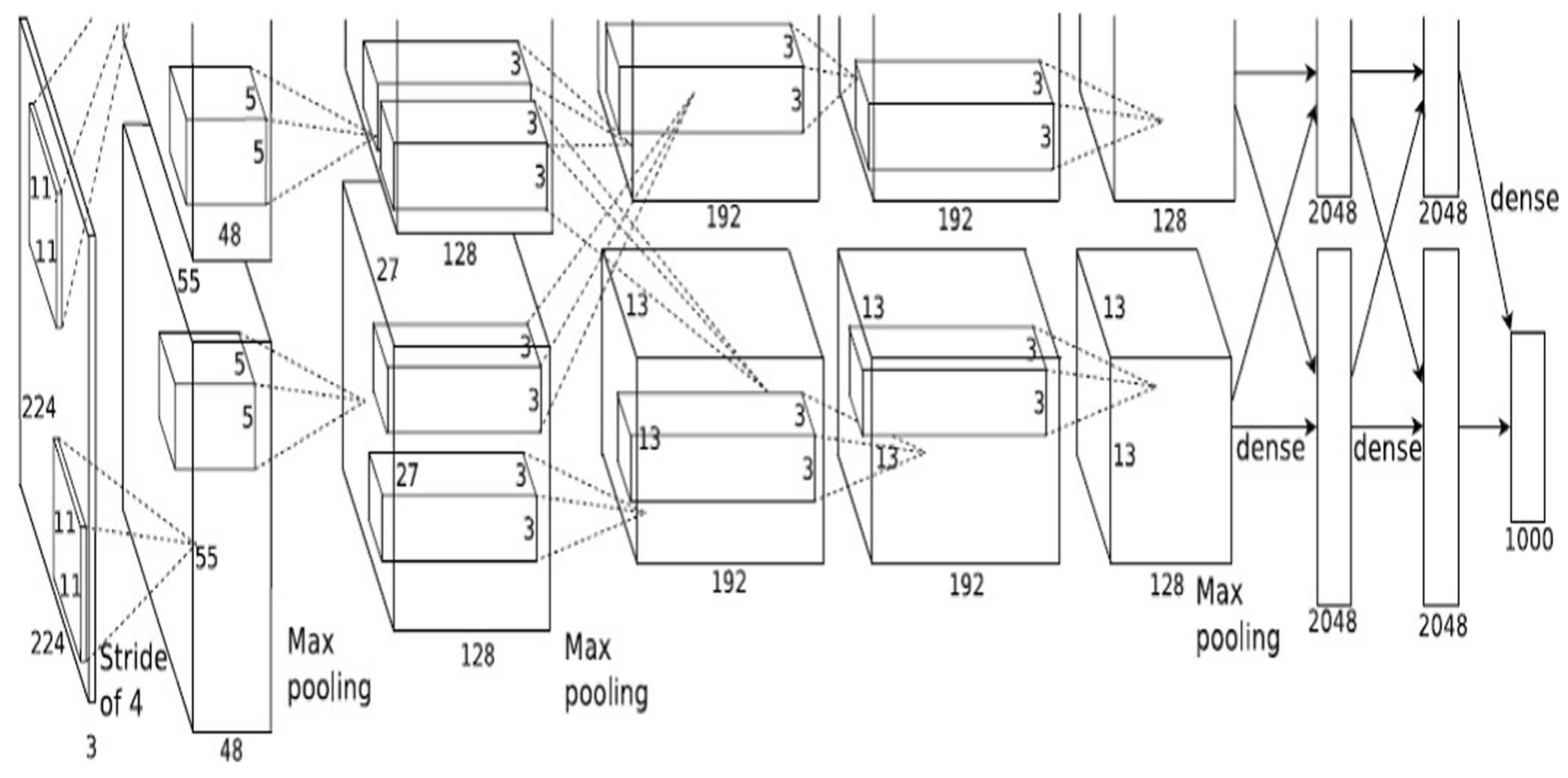
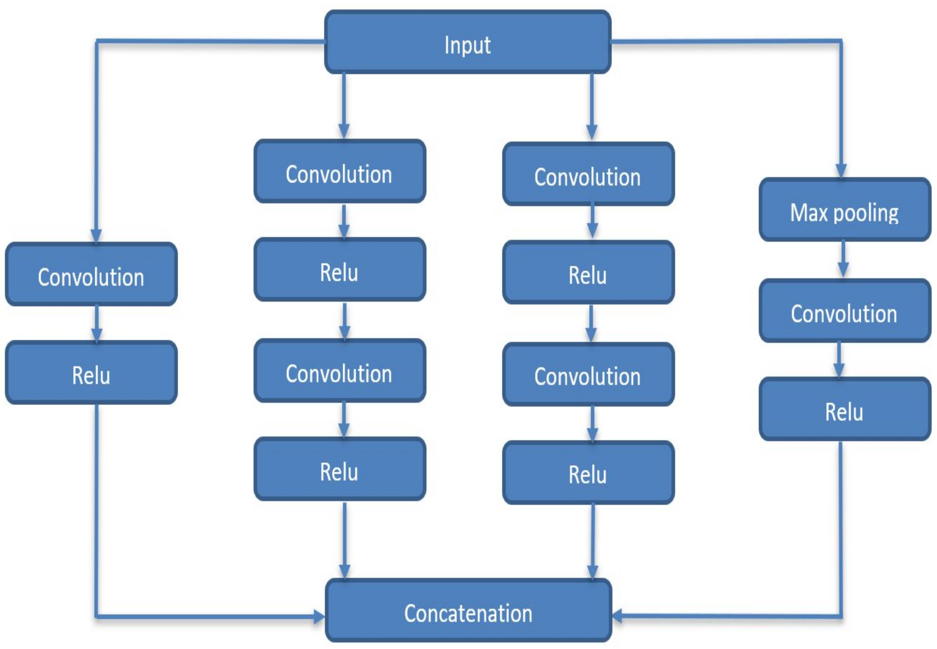
2.1. Deep Neural Networks
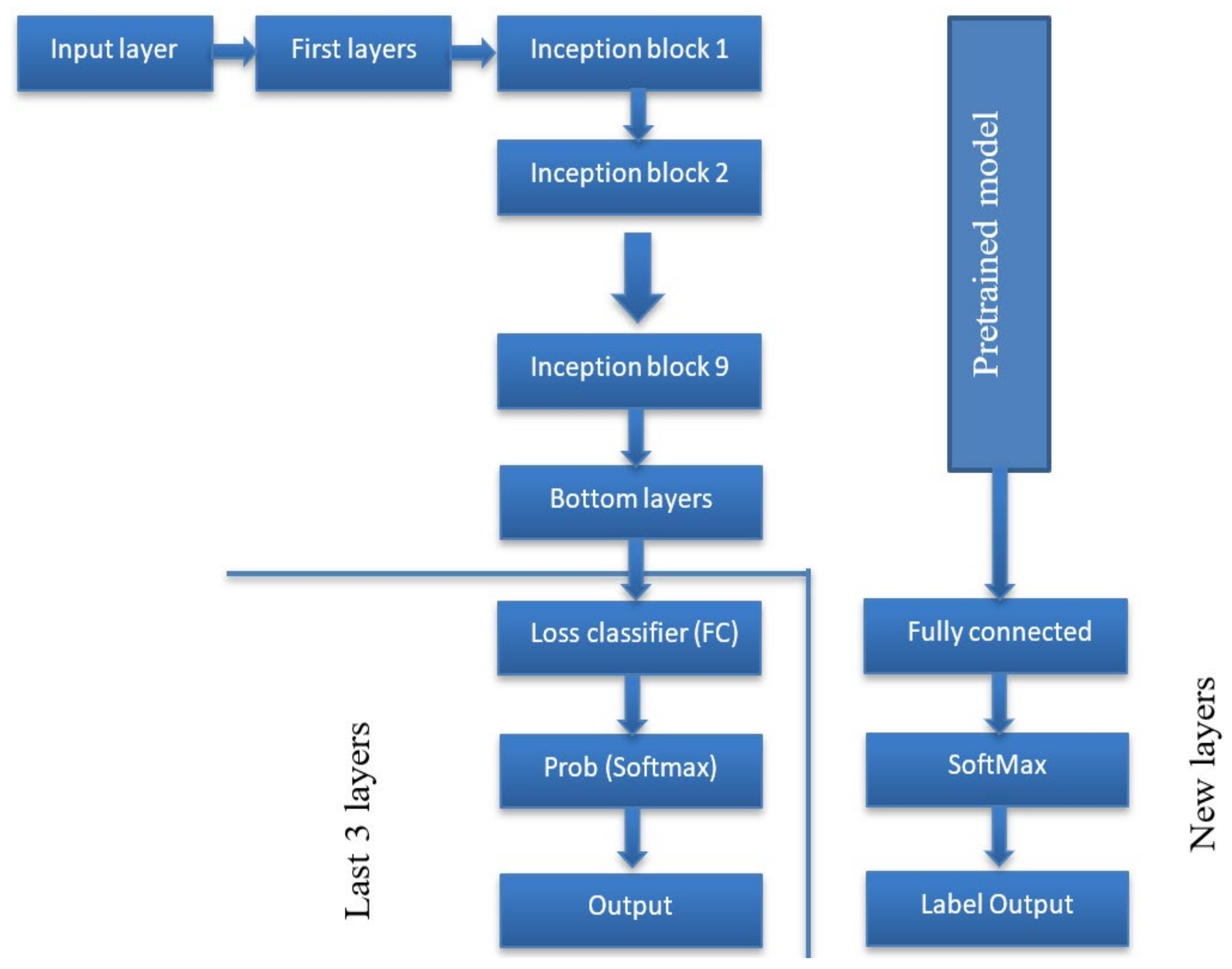
2.2. The Proposed Algorithm
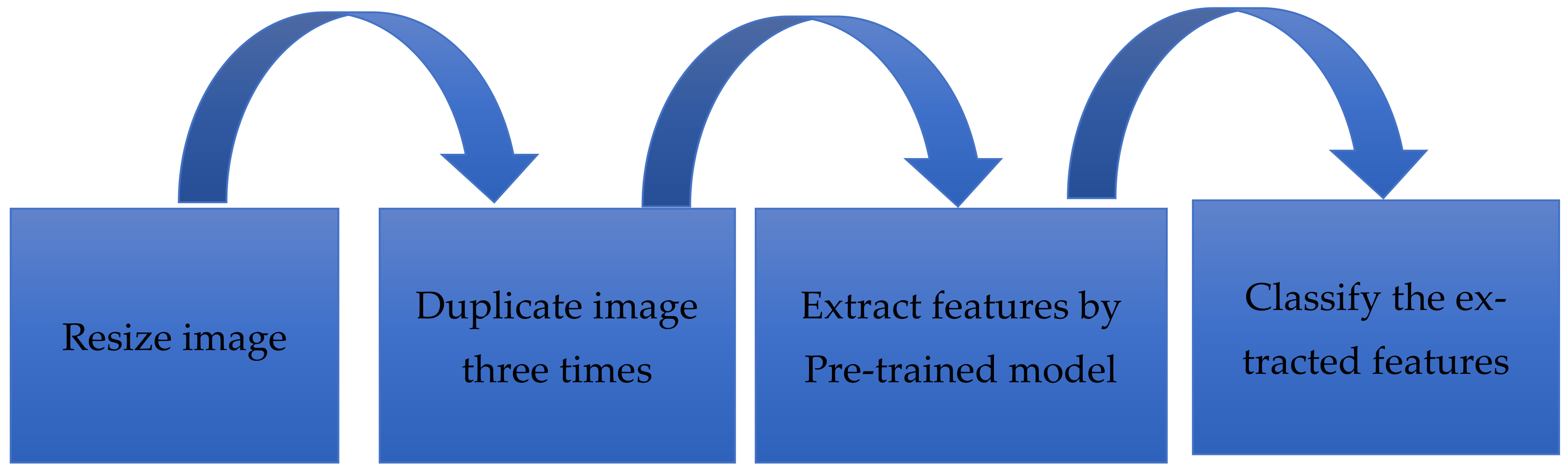
2.2.1. Preprocessing
| Algorithm 1 Duplication image for input channels | |
| Input: one-channel image | |
| Output: Three-channel image | |
| 1 | I = read the image |
| 2 | C = number of channels for (I) |
| 3 | If input image (C,1) |
| 4 | Concatenate arrays along specified dimensions (I, I, I) |
| 5 | Repeat step 1 to 4 for all images in the dataset |
| 6 | END |
| 7 | END |
2.2.2. Feature Extraction
2.2.3. Classification
3. Experiments
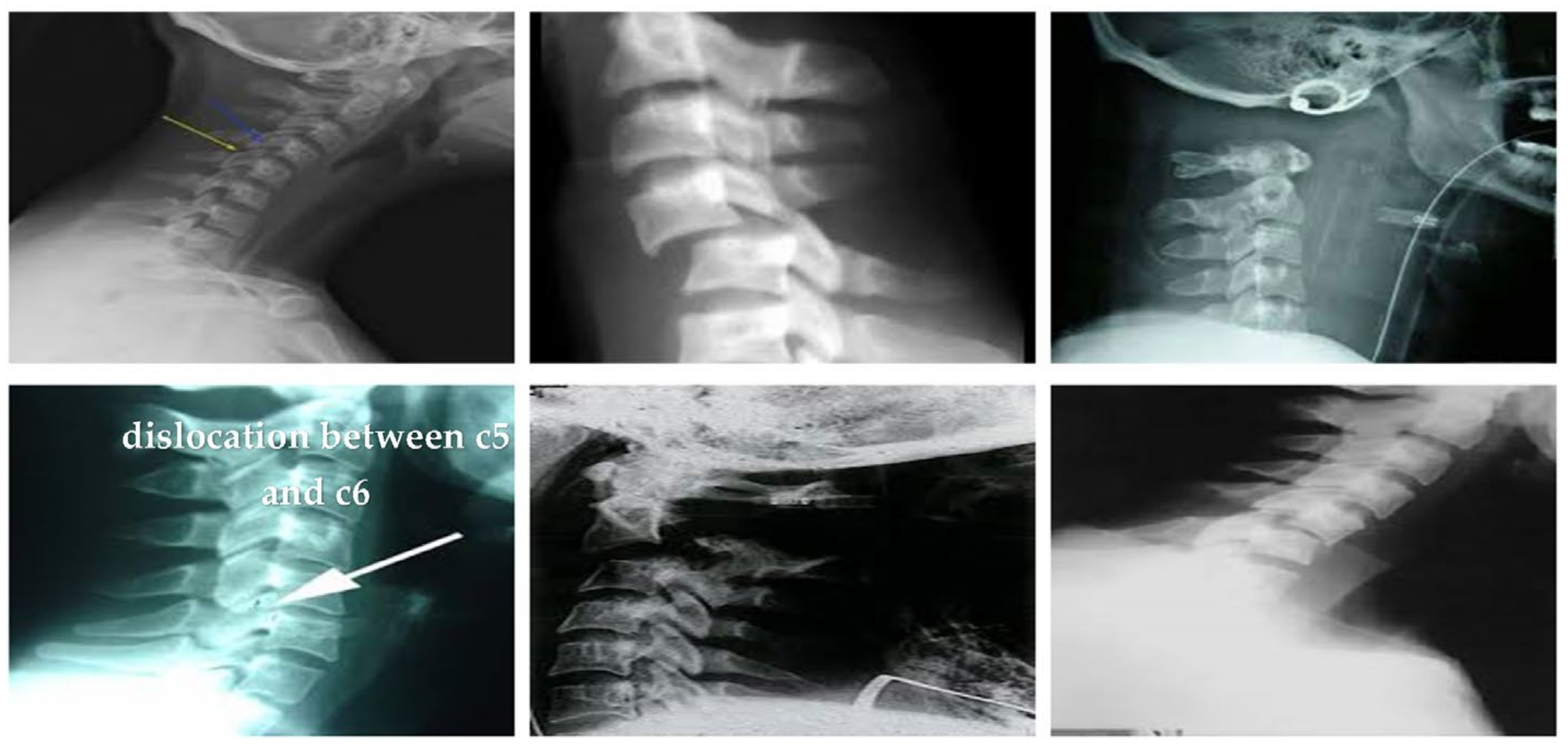
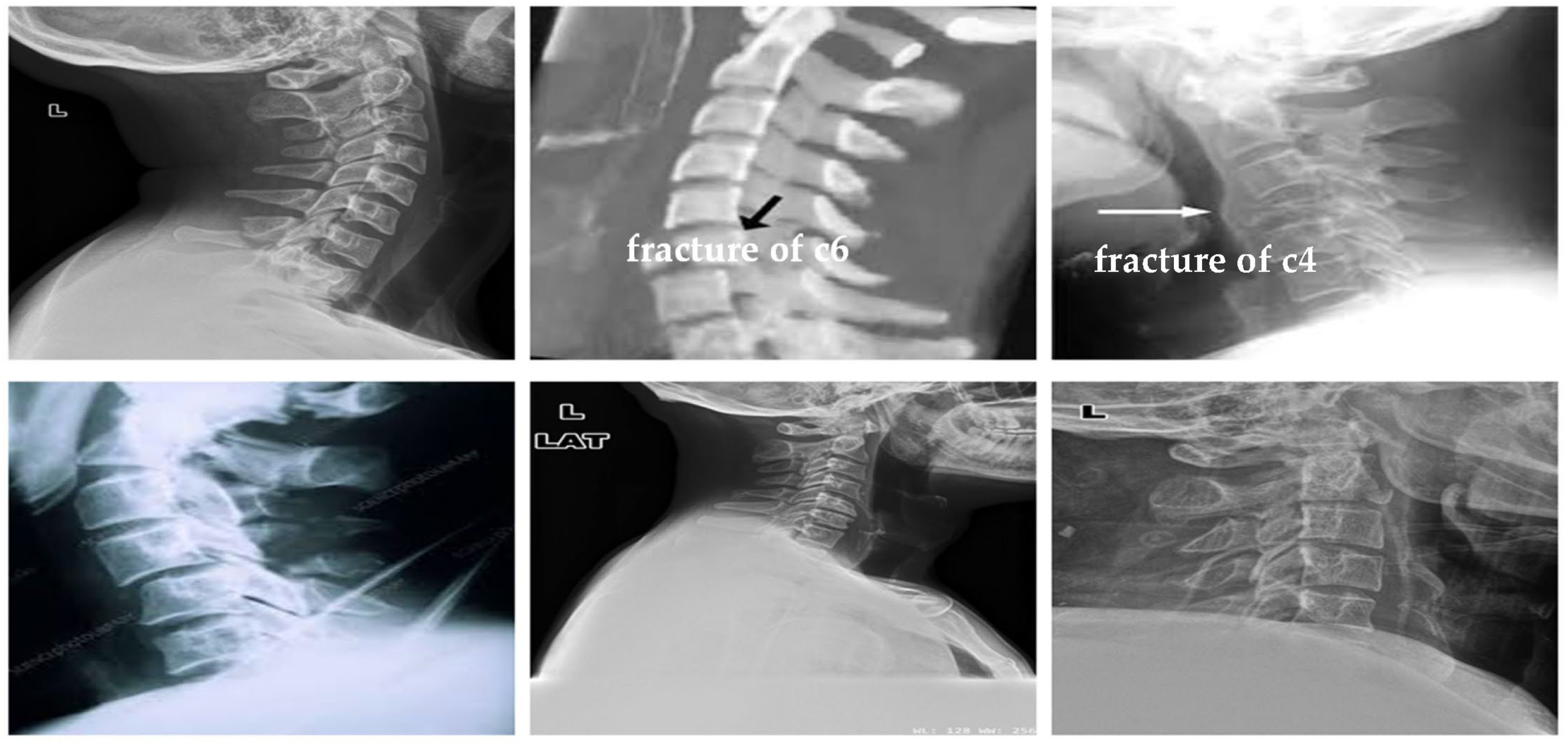
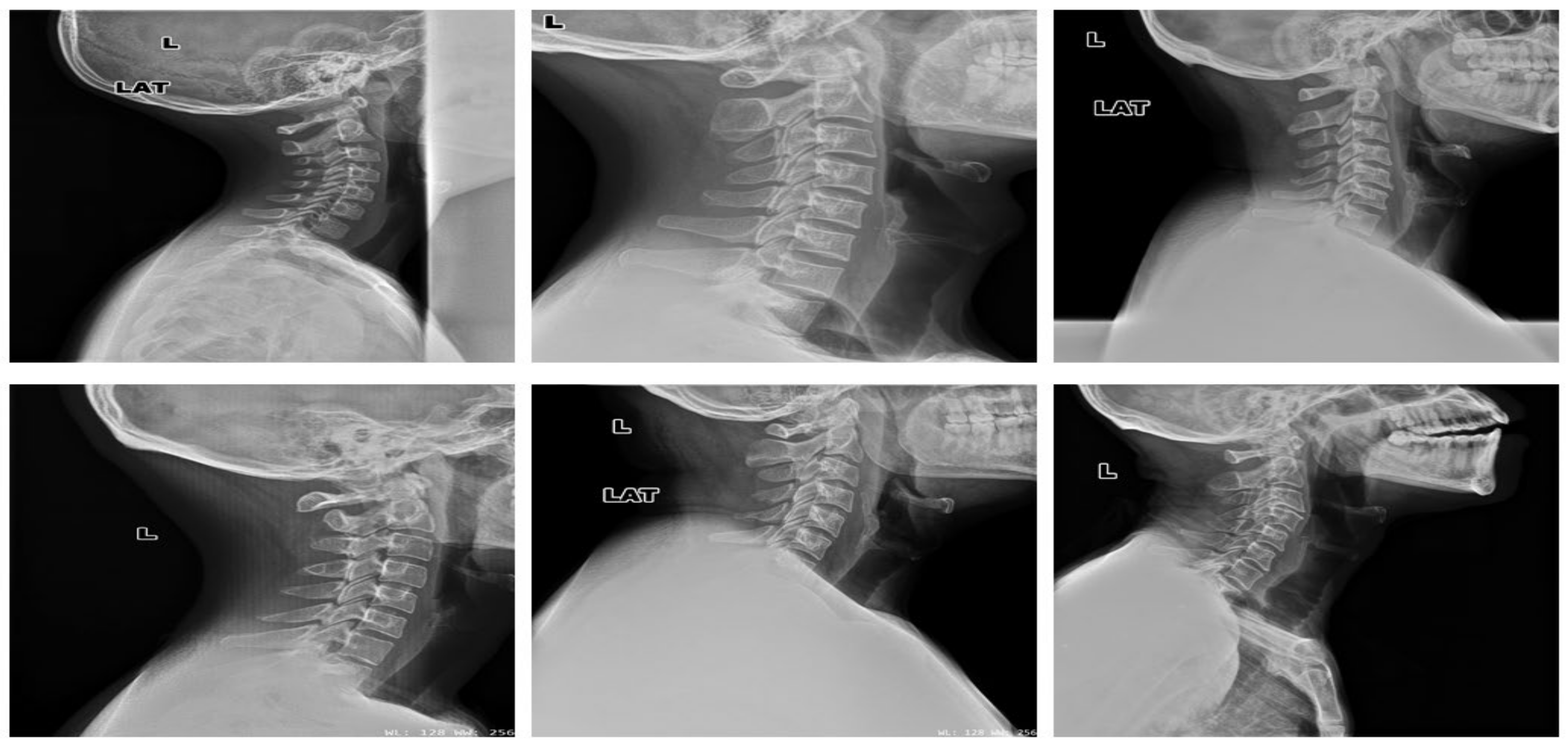
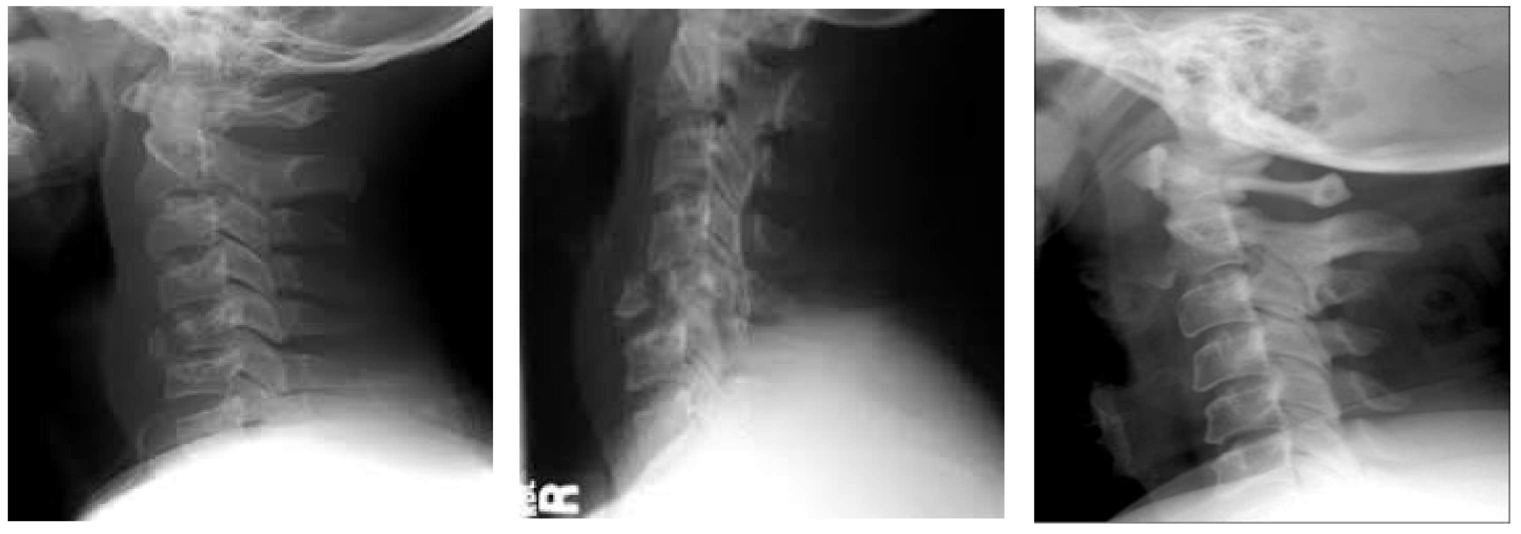
3.1. Datasets
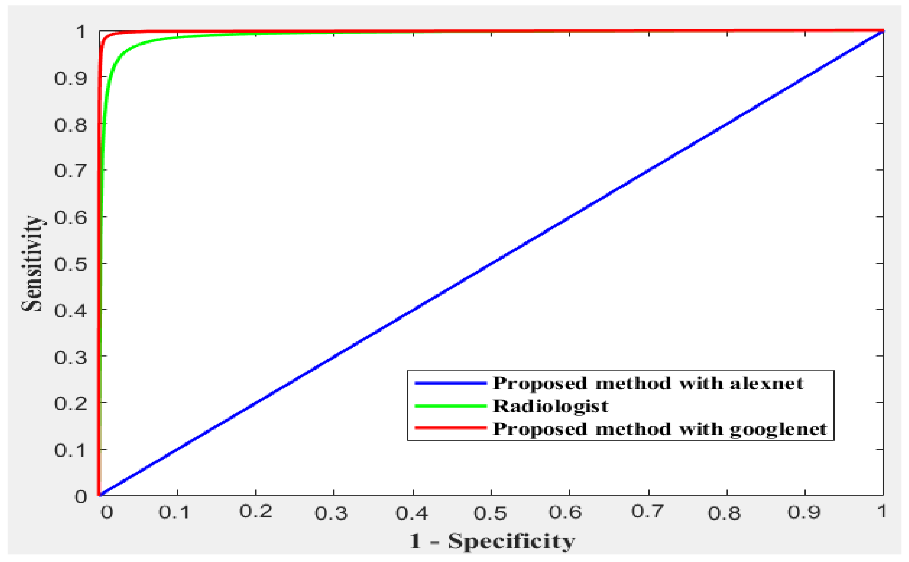
3.2. Performance Matrix
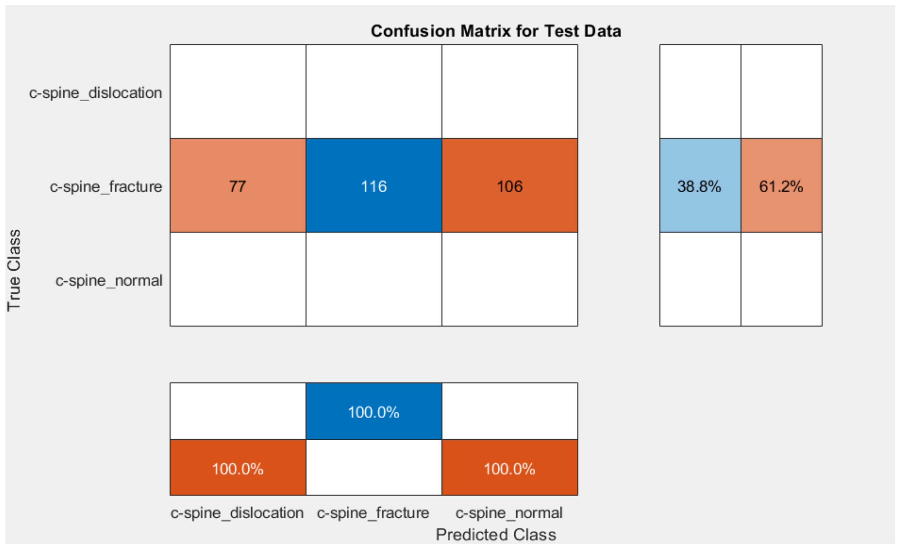
4. Results
4.1. Results and Discussion
4.1.1. Comparative Study
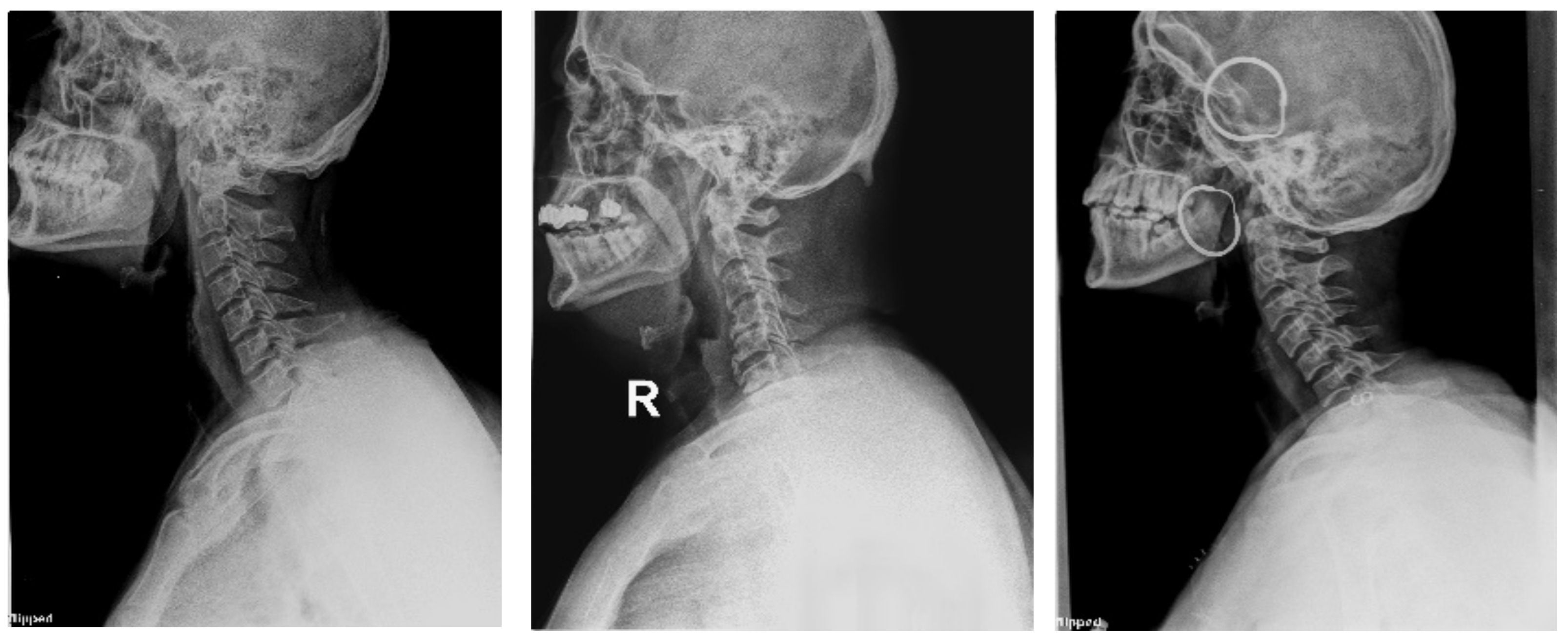
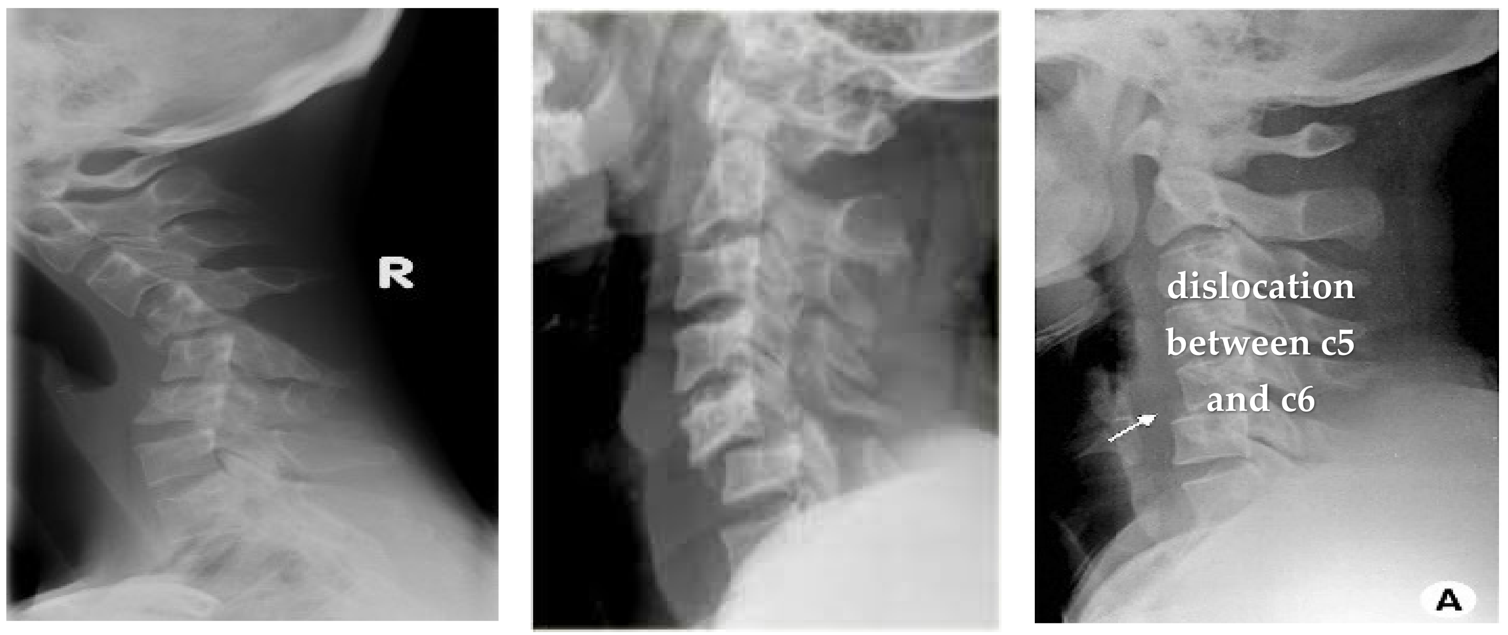
4.1.2. Clinical Case Study
4.1.3. Saliency Map
5. Discussion
6. Conclusions
Author Contributions
Funding
Institutional Review Board Statement
Informed Consent Statement
Data Availability Statement
Acknowledgments
Conflicts of Interest
Abbreviations
| AI | Artificial intelligence |
| ROI | Region of interest |
| CS | Cervical spine |
| CNN | Convolution neural networks |
| ReLU | Nonlinear rectified linear units |
| DCNN | Deep convolutional neural network |
| SGD | Stochastic gradient descent |
| LR | Learning rate |
| CCELF | Categorical cross-entropy loss function |
| ROC | Receiver operating characteristic |
References
- Daniels, J.M.; Hoffman, J.M. (Eds.) Common Musculoskeletal Problems: The Cervical Spine, A Handbook; Springer Science + Business Media: New York, NY, USA, 2010. [Google Scholar]
- Wang, T.Y.; Mehta, V.A.; Dalton, T.; Sankey, E.W.; Goodwin, C.R.; Karikari, I.O.; Shaffrey, C.I.; Than, K.D.; Abd-El-Barr, M.M. Biomechanics, evaluation, and management of subaxial cervical spine injuries: A comprehensive review of the literature. J. Clin. Neurosci. 2021, 83, 131–139. [Google Scholar] [CrossRef] [PubMed]
- Valladares, O.A.; Christenson, B.; Petersen, B.D. Radiologic Imaging of the Spine. In Spine Surgery Basics; Patel, V., Patel, A., Harrop, J., Burger, E., Eds.; Springer: Berlin/Heidelberg, Germany, 2014. [Google Scholar]
- Minja, F.J.; Mehta, K.Y.; Mian, A.Y. Current Challenges in the Use of Computed Tomography and MR Imaging in Suspected Cervical Spine Trauma. Neuroimaging Clin. N. Am. 2018, 28, 483–493. [Google Scholar] [CrossRef] [PubMed]
- Utheim, N.C.; Helseth, E.; Stroem, M.; Rydning, P.; Mejlænder-Evjensvold, M.; Glott, T.; Hoestmaelingen, C.T.; Aarhus, M.; Roenning, P.A.; Linnerud, H. Epidemiology of traumatic cervical spinal fractures in a general Norwegian population. Inj. Epidemiology 2022, 9, 1–13. [Google Scholar] [CrossRef]
- Wang, J.; Adam, E.M.; Eltorai, J.; Mason, D.; Wesley, D.; Reid, D.; Daniels, A.H. Variability in Treatment for Patients with Cervical Spine Fracture and Dislocation: An Analysis of 107,152 Patients. World Neurosurg. 2018, 114, 151–157. [Google Scholar] [CrossRef] [PubMed]
- Nishida, N.; Tripathi, S.; Mumtaz, M.; Kelkar, A.; Kumaran, Y.; Sakai, T.; Goel, V.K. Soft Tissue Injury in Cervical Spine Is a Risk Factor for Intersegmental Instability: A Finite Element Analysis. World Neurosurg. 2022, 164, e358–e366. [Google Scholar] [CrossRef]
- Beauséjour, M.-H.; Petit, Y.; Wagnac, É.; Melot, A.; Troude, L.; Arnoux, P.-J. Cervical spine injury response to direct rear head impact. Clin. Biomech. 2021, 92, 105552. [Google Scholar] [CrossRef]
- Dennis, C. The Vulnerable Neck: What Forensic Audiologists Should Know. Hear. J. 2020, 73, 46–47. [Google Scholar]
- Danka, D.; Szloboda, P.; Nyary, I.; Bojtar, I. The fracture of the human cervical spine. Mater. Today: Proc. 2022, 62, 2495–2501. [Google Scholar] [CrossRef]
- Gao, W.; Wang, B.; Hao, D.; Ziqi, Z.; Guo, H.; Hui, L.; Kong, L. Surgical Treatment of Lower Cervical Fracture-Dislocation with Spinal Cord Injuries by Anterior Approach: 5- to 15-Year Follow-Up. World Neurosurg. 2018, 115, 137–145. [Google Scholar] [CrossRef]
- Small, J.E.; Osler, P.; Paul, A.B.; Kunst, M. Cervical Spine Fracture Detection Using a Convolutional Neural Network. AJNR Am. J. Neuroradiol. 2021, 42, 1341–1347. [Google Scholar] [CrossRef]
- AlGhaithi, A.; Al Maskari, S. Artificial intelligence application in bone fracture detection. J. Musculoskelet. Surg. Res. 2021, 5, 4–9. [Google Scholar] [CrossRef]
- Kriza, C.; Amenta, V.; Zenié, A.; Panidis, D.; Chassaigne, H.; Urbán, P.; Holzwarth, U.; Sauer, A.V.; Reina, V.; Griesinger, C.B. Artificial intelligence for imaging-based COVID-19 detection: Systematic review comparing added value of AI versus human readers. Eur. J. Radiol. 2021, 145, 110028. [Google Scholar] [CrossRef] [PubMed]
- Sakib, A.; Siddique M d Khan, M.; Yasmin, N.; Aziz, A.; Chowdhury, M.; Tasawar, I. Transfer Learning Based Method for Automatic COVID-19 Cases Detection in Chest X-Ray Images. In Proceedings of the 2nd International Conference on Smart Electronics and Communication (ICOSEC), Trichy, India, 7–9 October 2021; pp. 890–895. [Google Scholar]
- Wu, J.; Gur, Y.; Karargyris, A.; Syed, A.B.; Boyko, O.; Moradi, M.; Mahmood, T. Automatic Bounding Box Annotation of Chest X-Ray Data for Localization of Abnormalities. In Proceedings of the IEEE 17th International Symposium on Biomedical Imaging (ISBI), Iowa City, Iowa, USA, 3–7 April 2020; pp. 799–803. [Google Scholar]
- Adams, S.J.; Henderson RD, E.; Yi, X.; Babyn, P. Artificial Intelligence Solutions for Analysis of X-ray Images. Can. Assoc. Radiol. J. 2021, 72, 60–72. [Google Scholar] [CrossRef]
- Rainey, C.; McConnell, J.; Hughes, C.; Bond, R.; McFadden, S. Artificial intelligence for diagnosis of fractures on plain radiographs: A scoping review of current literature. Intell. Med. 2021, 5, 100033. [Google Scholar] [CrossRef]
- Jones, R.M.; Sharma, A.; Hotchkiss, R.; Sperling, J.W.; Hamburger, J.; Ledig, C.; O’Toole, R.; Gardner, M.; Venkatesh, S.; Roberts, M.M.; et al. Assessment of a deep-learning system for fracture detection in musculoskeletal radiographs. NPJ Digit. Med. 2020, 3, 144. [Google Scholar] [CrossRef]
- Hardalaç, F.; Uysal, F.; Peker, O.; Çiçeklidağ, M.; Tolunay, T.; Tokgöz, N.; Kutbay, U.; Demirciler, B.; Mert, F. Fracture Detection in Wrist X-ray Images Using Deep Learning-Based Object Detection Models. Sensors 2022, 22, 1285. [Google Scholar] [CrossRef]
- Lu, S.; Wang, S.; Wang, G. Automated universal fractures detection in X-ray images based on deep learning approach. Multimed. 2022, 81, 44487–44503. [Google Scholar] [CrossRef]
- Salehinejad, S.; Edward, H.; Hui-Ming, L.; Priscila, C.; Oleksandra, S.; Monica, T.; Zamir, M.; Suthiphosuwan, S.; Bharatha, A.; Yeom, K.; et al. Deep Sequential Learning For Cervical Spine Fracture Detection On Computed Tomography Imaging. In Proceedings of the 2021 IEEE 18th International Symposium on Biomedical Imaging (ISBI), Nice, France, 13–16 April 2021; pp. 1911–1914. [Google Scholar]
- Hosny, K.M.; Kassem, M.A. Refined Residual Deep Convolutional Network for Skin Lesion Classification. J Digit. Imaging 2022, 35, 258–280. [Google Scholar] [CrossRef]
- Kassem, M.; Hosny, K.; Damaševičius, R.; Eltoukhy, M. Machine Learning and Deep Learning Methods for Skin Lesion Classification and Diagnosis: A Systematic Review. Diagnostics 2021, 11, 1390. [Google Scholar] [CrossRef]
- Hosny, K.M.; Kassem, M.A.; Fouad, M.M. Skin melanoma classification using ROI and data augmentation with deep convolutional neural networks. Multimed. Tools Appl. 2020, 79, 24029–24055. [Google Scholar] [CrossRef]
- Prusa, J.D.; Khoshgoftaar, T.M. Improving deep neural network design with new text data representations. J. Big Data 2017, 4, 7. [Google Scholar] [CrossRef] [Green Version]
- Yosinski, J.; Clune, J.; Bengio, Y.; Lipson, H. How transferable are features in deep neural networks? Adv. Neural Inf. Process. Syst. 2014, 27, 3320–3328. [Google Scholar]
- Brinker, T.J.; Hekler, A.; Utikal, J.S.; Grabe, N.; Schadendorf, D.; Klode, J.; Kalle, C. Skin cancer classification using convolutional neural networks: Systematic review. J. Med. Internet Res. 2018, 20, e11936. [Google Scholar] [CrossRef]
- LeCun, Y.; Bottou, L.; Bengio, Y.; Haffner, P. Gradient-based learning applied to document recognition. Proc. IEEE 1998, 86, 2278–2324. [Google Scholar] [CrossRef] [Green Version]
- Suraj, S.; Kiran, S.R.; Reddy, M.K.; Nikita, P.; Srinivas, K.; Venkatesh, B.R. A taxonomy of deep convolutional neural nets for computer vision. Front. Robot. AI 2016, 2, 1–36. [Google Scholar]
- Tan, C.; Sun, F.; Kong, T.; Zhang, W.; Yang, C.; Liu, C. A survey on deep transfer learning. In Proceedings of the International Conference on Artificial Neural Networks, Rhodes, Greece, 4–7 October 2018; Springer: Berlin/Heidelberg, Germany, 2018. [Google Scholar]
- Donahue, J.; Jia, Y.; Vinyals, O.; Hoffman, J.; Zhang, N.; Tzeng, E.; Darrell, T.D. A deep convolutional activation feature for generic visual recognition. In Proceedings of the International Conference on Machine Learning, Beijing, China, 21–26 June 2014. [Google Scholar]
- Zeiler, M.D.; Fergus, R. Stochastic pooling for regularization of deep convolutional neural networks. In Proceedings of the 1st International Conference on Learning Representations, Scottsdale, AZ, USA, 2–4 May 2013. [Google Scholar]
- Krizhevsky, A.; Sutskever, I.; Hinton, G. ImageNet Classification with Deep Convolutional Neural Networks. Proc. Neural Inf. Process. Syst. (NIPS) 2012, 1, 1097–1105. [Google Scholar] [CrossRef] [Green Version]
- Szegedy, C.; Liu, W.; Jia, Y.; Sermanet, P.; Reed, S.; Anguelov, D.; Erhan, D.; Vanhoucke, V.; Rabinovich, A. Going deeper with convolutions. In Proceedings of the IEEE Conference on Computer Vision and Pattern Recognition (CVPR), Boston, MA, USA, 7–12 June 2015; pp. 1–9. [Google Scholar]
- Available online: https://www.kaggle.com/datasets/pardonndlovu/chestpelviscspinescans/metadata?select=c-spine_normal (accessed on 5 October 2022).
- Fawcett, T. An Introduction to ROC analysis. Pattern Recogn. Lett. 2006, 27, 861–874. [Google Scholar] [CrossRef]


| Accuracy | Sensitivity | Specificity | Precision | F1-Score | |
|---|---|---|---|---|---|
| Radiologist | 95% | 93% | 96% | 87% | |
| The proposed method with AlexNet | 59.2 | 33.33 | 66.67 | 13.0 | 18.67 |
| The proposed method with GoogleNet | 99.55% | 99.33% | 99.66% | 99.33% | 99.67 |
| No. of Correctly Recognized | No. of Wrongly Recognized | |
|---|---|---|
| The proposed method | 60 (92.16) | 8 (1.84%) |
| Radiologist | 66 (97.1%) | 2 (2.9%) |
| Orthopedic Surgeon | 67 (98.5%) | 1 (1.5%) |
Disclaimer/Publisher’s Note: The statements, opinions and data contained in all publications are solely those of the individual author(s) and contributor(s) and not of MDPI and/or the editor(s). MDPI and/or the editor(s) disclaim responsibility for any injury to people or property resulting from any ideas, methods, instructions or products referred to in the content. |
© 2023 by the authors. Licensee MDPI, Basel, Switzerland. This article is an open access article distributed under the terms and conditions of the Creative Commons Attribution (CC BY) license (https://creativecommons.org/licenses/by/4.0/).
Share and Cite
Naguib, S.M.; Hamza, H.M.; Hosny, K.M.; Saleh, M.K.; Kassem, M.A. Classification of Cervical Spine Fracture and Dislocation Using Refined Pre-Trained Deep Model and Saliency Map. Diagnostics 2023, 13, 1273. https://doi.org/10.3390/diagnostics13071273
Naguib SM, Hamza HM, Hosny KM, Saleh MK, Kassem MA. Classification of Cervical Spine Fracture and Dislocation Using Refined Pre-Trained Deep Model and Saliency Map. Diagnostics. 2023; 13(7):1273. https://doi.org/10.3390/diagnostics13071273
Chicago/Turabian StyleNaguib, Soaad M., Hanaa M. Hamza, Khalid M. Hosny, Mohammad K. Saleh, and Mohamed A. Kassem. 2023. "Classification of Cervical Spine Fracture and Dislocation Using Refined Pre-Trained Deep Model and Saliency Map" Diagnostics 13, no. 7: 1273. https://doi.org/10.3390/diagnostics13071273