
Interpretable Machine Learning Techniques in ECG-Based Heart Disease Classification: A Systematic Review

 , , and
Abstract
:1. Introduction
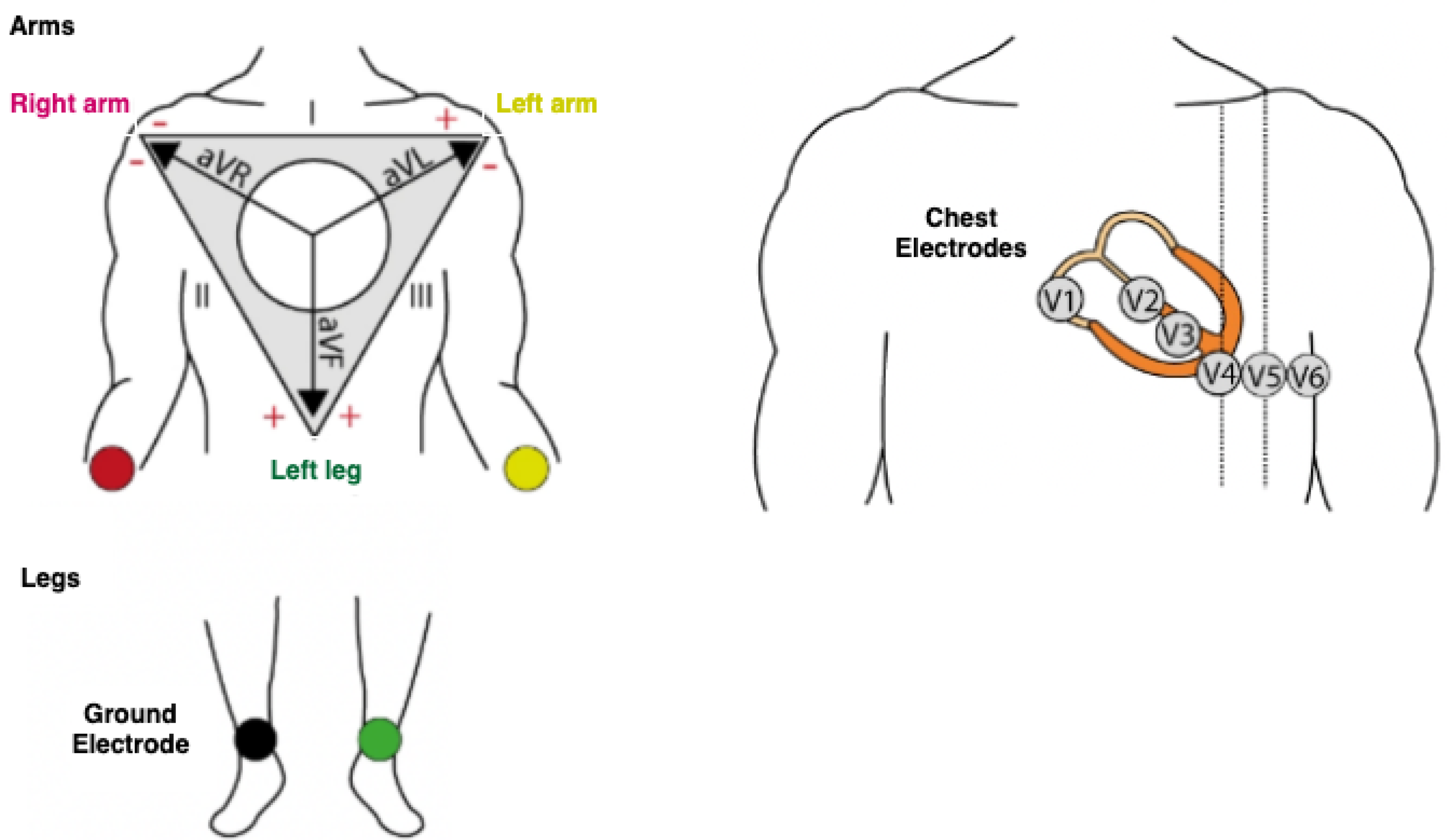
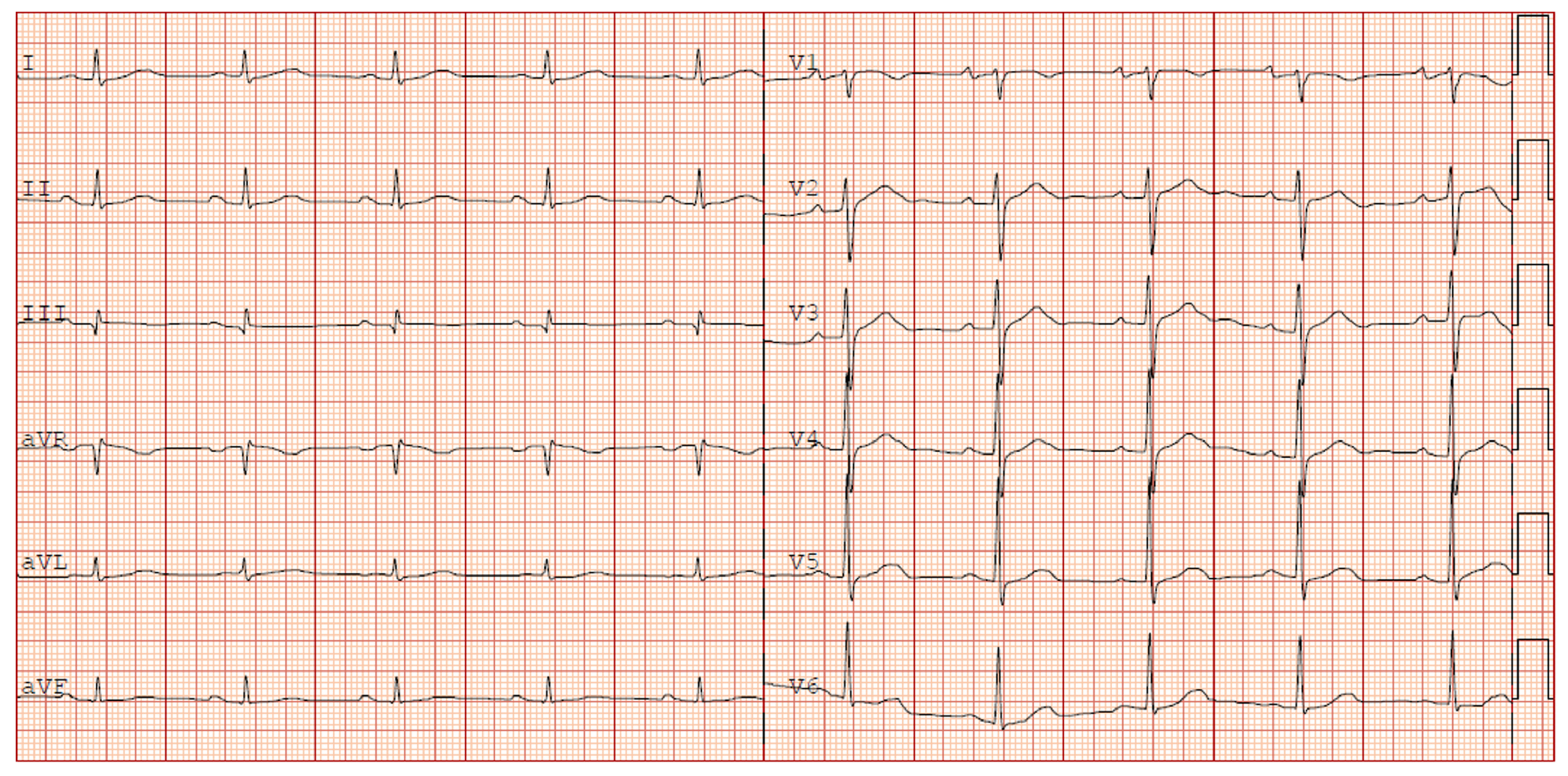
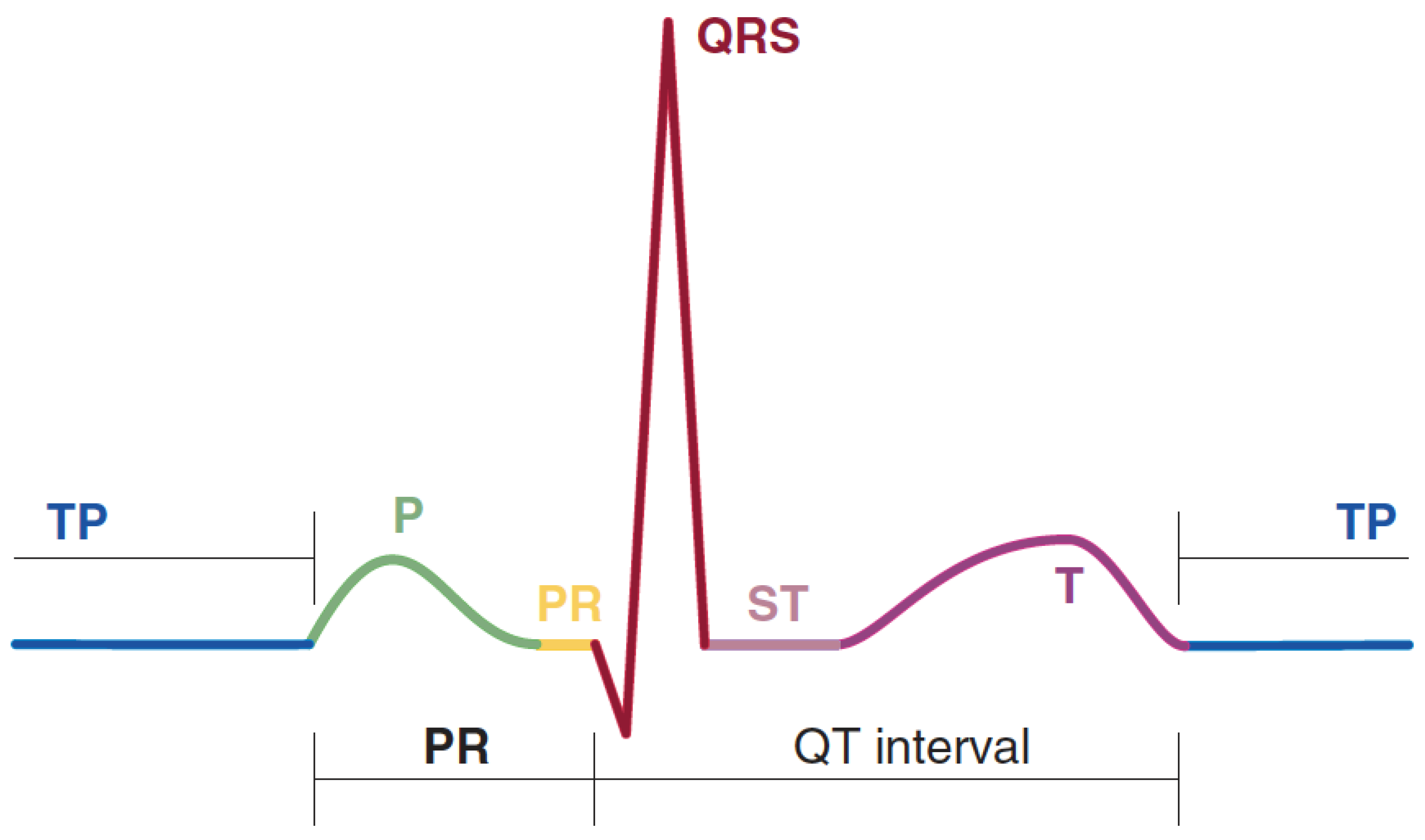
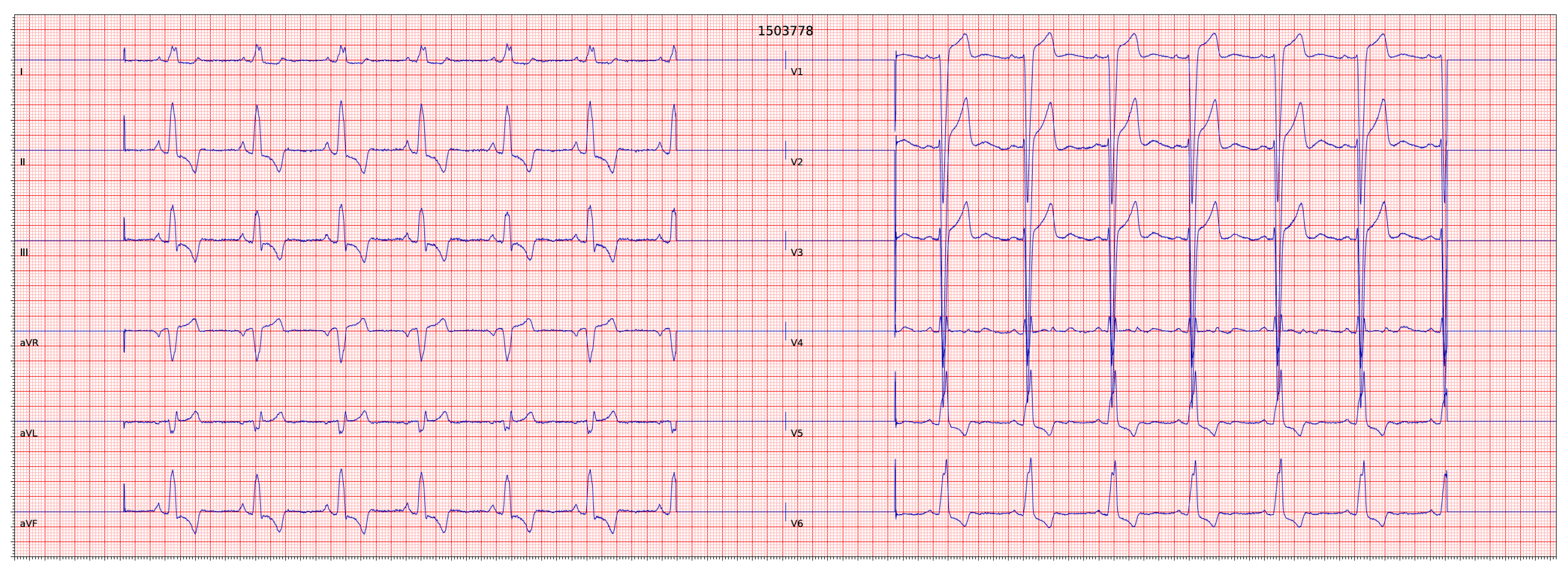
1.1. ECG Signal
1.2. Machine Learning: In an ECG Signal Classification Prescriptive
2. Related Work
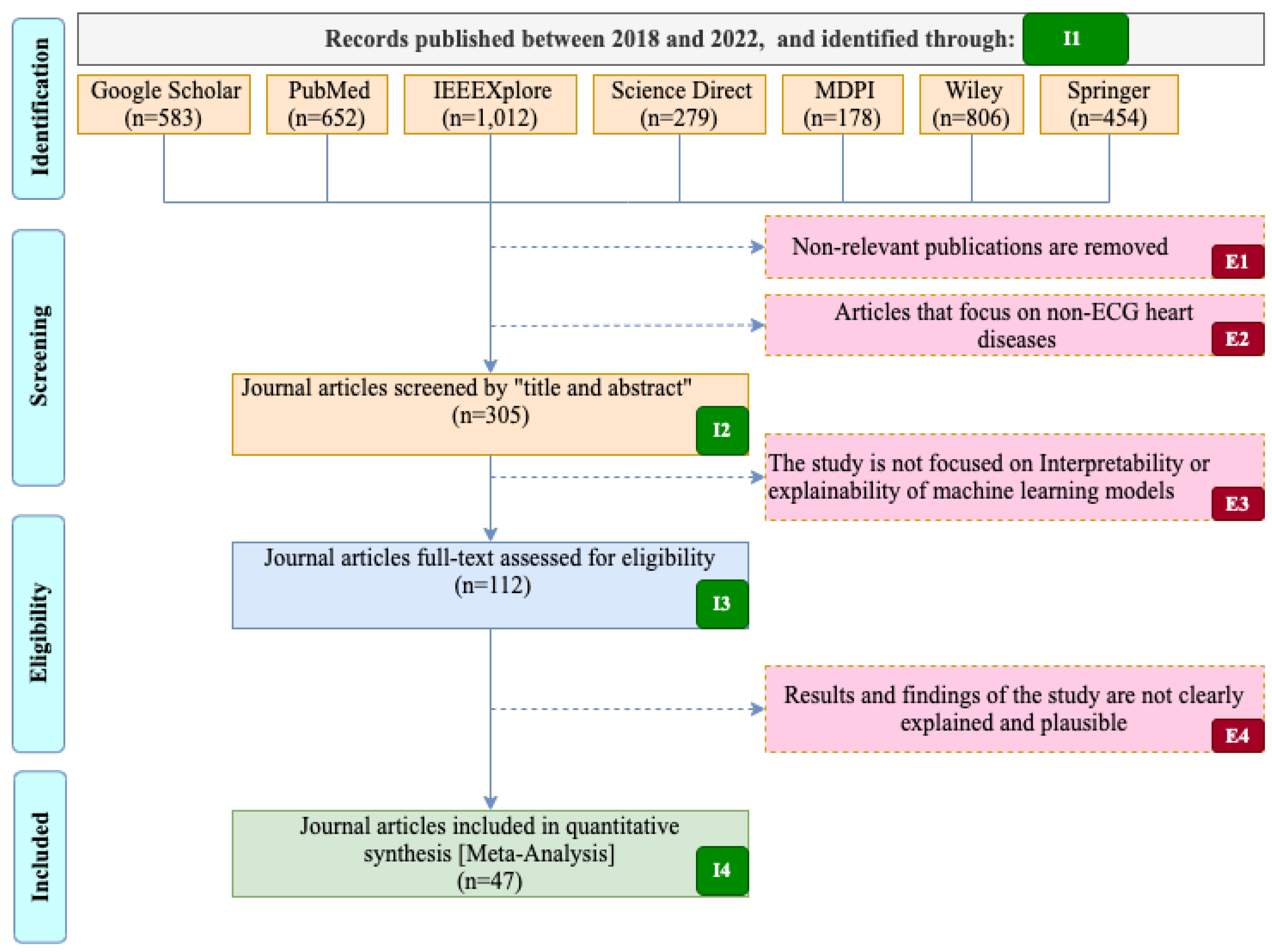
3. Method
- Defining the research questions;
- Based on the research questions, retrieving some keywords to create proper search strings;
- Identifying the databases for performing the search using the created search strings;
- Setting filtering criteria, including the chronological period, the quality, and the type of literature to be included in the review;
- Skimming titles and abstracts to avoid unrelated articles and duplicates from the pool of papers;
- Defining more detailed suitability criteria and using them in a full paper reading of the outlived papers from the previous steps;
- Analyzing and interpreting the outlived articles from all the filtering procedures in line with research questions defined in the beginning;
- Reporting and evaluating the systematic review.
3.1. Research Question
3.2. Search Strategy
- Google Scholar, a scholarly literature search engine that encompasses a wide variety of disciplines and publisher databases;
- PubMed, a database consisted of a large number of literary studies in the biomedical field, primarily from the MEDLINE database;
- IEEE Xplore, this database contains high-quality technical literature in the fields of electrical engineering, electronics, computer science, and other related fields;
- ScienceDirect, using this database, access to journals and technical articles published by Elsevier is possible;
- MDPI, a publisher of open-access peer-reviewed scientific journals;
- Wiley Online Library, this is a repository of published articles in various disciplines, including computational, intelligent systems, and life sciences;
- SpringerLink, through this database, we can access scientific articles published by Springer Nature.
4. Heart Electrocardiogram Diagnosis Datasets

| Dataset | # of Lead | # of Records | Annotation Type | # of Classes [Including Normal] | Samp. Freq. (Hz) | Website URL 1 |
|---|---|---|---|---|---|---|
| MIT-BIH Arrhythmia database [48] | 2 leads | 48 two-channel half-hour recordings |
|
| 360 | https://physionet.org/content/mitdb/1.0.0/ |
| MIT-BIH Atrial Fibrillation Database [49] | 2 leads | 25 two-channel 10-h recordings |
|
| 250 | https://physionet.org/content/afdb/1.0.0/ |
| MIT-BIH Normal Sinus Rhythm Database [50] | 2 leads | 18 two-channel 24-h recordings |
|
| 128 | https://physionet.org/content/nsrdb/1.0.0/ |
| BIDMC-Congestive Heart failure (CHF) database [51] | 2 leads | 15 two-channel 20-h recordings |
|
| 250 | https://physionet.org/content/chfdb/1.0.0/ |
| Normal sinus rhythm RR interval database [52] | 2 leads | 54 two-channel half-hour recordings |
|
| 128 | https://physionet.org/content/nsr2db/1.0.0/ |
5. Interpretable Machine Learning (IML)
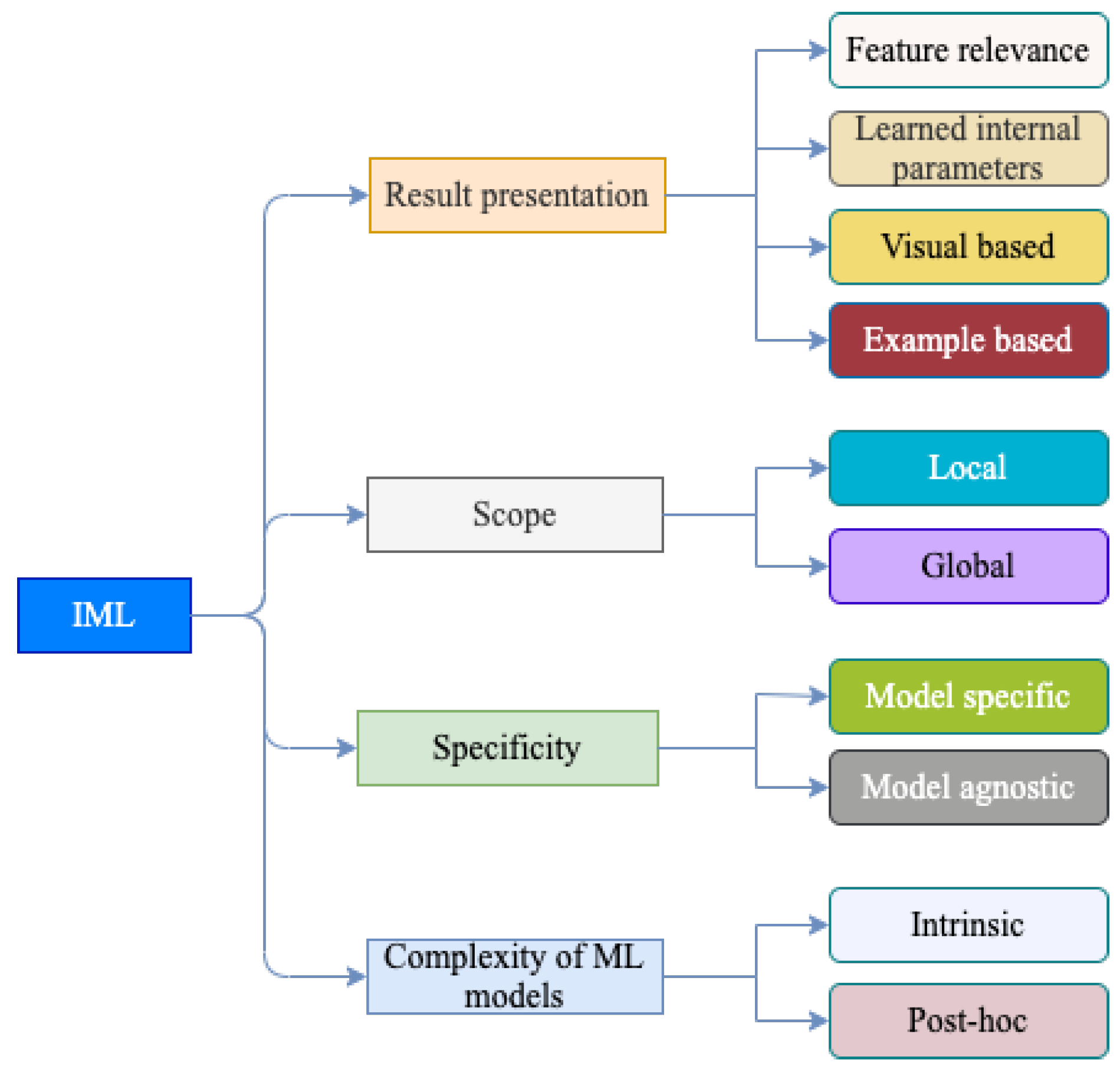
5.1. Taxonomy of IML
5.2. Result Presentation in IML
5.2.1. Interpretation Result Presentation Using Feature Relevance
SHapley Additive exPlanations (SHAP)
Local Interpretable Model-Agnostic Explanations (LIME)
Permutation Feature Importance (PFI)
5.2.2. Interpretation Result Presentation by Learned Internal Parameters of the Model
5.2.3. Interpretation Result Presentation through Visual Explanation
Class Activation Maps
Saliency Maps
Layer-Wise Relevance Propagation (LRP)
Occlusion Map
Attention Mechanisms
5.2.4. Interpretation Result Presentation Using an Example-Based Explanation
5.3. Scope of IML Techniques
5.4. Specificity of IML Techniques
5.5. Complexity of ML Models
5.6. Summary of Taxonomy of IML Techniques
6. Performance Evaluation of Interpretability Methods
6.1. Visual Observation
6.2. Feature Effect
6.3. Attention Score
6.4. Jaccard Index
6.5. Performance Decrease
7. Discussion
8. Challenges and Future Direction
9. Conclusions
- RQ1: Are there any freely available heart ECG signal datasets? What are their characteristics?As discussed in Section 4, there are several annotated heart disease ECG tracing datasets in repositories. These datasets are composed of single-lead and 12-lead ECG tracings (sampled at different sampling frequencies). In addition, the number of recordings in the dataset and classes annotating heart disease also vary. Moreover, the disease classes in these datasets are not balanced. Furthermore, some annotations are at the heartbeat level and others involve whole ECG tracing. Above all, these repositories are not fit for developing and testing IML methods as they do not have clinical reasoning, such as location and morphological manifestations of abnormalities in ECG tracing.
- RQ2: What are IML techniques and commonly investigated interpretable techniques in ECG signal-based heart disease diagnoses?As discussed in Section 5, we identified IML methods and categorized them in a taxonomy to discuss their working principles and spot their gaps. These IML methods attempt to localize the regions of an ECG signal that contributes the most to the classification process. However, they have limitations, such as computational complexity, gradient saturation problem, lack of generalization, and susceptibility to input ECG signal perturbation.
- RQ3: What is the overall progress and performance of IML algorithms in providing evidence-based heart disease diagnoses?The proposed methods in the literature explain the ML model’s output in terms of visual presentation, feature importance, internal ML model parameters, and factual examples. However, the explanations provided are not easily understandable. In addition, due to the lack of commonly agreed-upon performance evaluation metrics and ground truth, the methods are not rigorously evaluated.
- RQ4: Are there any limitations and challenges in IML-based heart disease classifications?Section 8 clearly identifies the existing challenges, such as the absence of standardized evaluation metrics, lack of well-defined use cases, explanation clarity, and ground truth dataset. In addition, future directions are highlighted.
Author Contributions
Funding
Data Availability Statement
Conflicts of Interest
References
- Fact Sheet: Cardiovascular Diseases. Available online: https://www.who.int/news-room/fact-sheets/detail/cardiovascular-diseases-(cvds) (accessed on 23 May 2022).
- Morris, F. ABC of Clinical Electrocardiography; Blackwell Pub: Oxford, UK, 2008. [Google Scholar]
- Manda, Y.R.; Baradhi, K.M. Cardiac Catheterization Risks and Complications; StatPearls Publishing: Treasure Island, FL, USA, 2021. [Google Scholar]
- Jørgensen, M.E.; Andersson, C.; Nørgaard, B.L.; Abdulla, J.; Shreibati, J.B.; Torp-Pedersen, C.; Gislason, G.H.; Shaw, R.E.; Hlatky, M.A. Functional Testing or Coronary Computed Tomography Angiography in Patients With Stable Coronary Artery Disease. J. Am. Coll. Cardiol. 2017, 69, 1761–1770. [Google Scholar] [CrossRef] [PubMed]
- Syed, I.S.; Glockner, J.F.; Feng, D.; Araoz, P.A.; Martinez, M.W.; Edwards, W.D.; Gertz, M.A.; Dispenzieri, A.; Oh, J.K.; Bellavia, D.; et al. Role of Cardiac Magnetic Resonance Imaging in the Detection of Cardiac Amyloidosis. JACC Cardiovasc. Imaging 2010, 3, 155–164. [Google Scholar] [CrossRef]
- Pannu, J.; Poole, S.; Shah, N.; Shah, N.H. Assessing Screening Guidelines for Cardiovascular Disease Risk Factors using Routinely Collected Data. SCient. Rep. 2017, 7, 6488. [Google Scholar] [CrossRef] [PubMed] [Green Version]
- Iragavarapu, T.; Radhakrishna, T.; Babu, K.J.; Sanghamitra, R. Acute coronary syndrome in young—A tertiary care centre experience with reference to coronary angiogram. J. Pract. Cardiovasc. Sci. 2019, 5, 18. [Google Scholar] [CrossRef]
- Rafie, N.; Kashou, A.H.; Noseworthy, P.A. ECG Interpretation: Clinical Relevance, Challenges, and Advances. Hearts 2021, 2, 505–513. [Google Scholar] [CrossRef]
- Cook, D.A.; Oh, S.Y.; Pusic, M.V. Accuracy of Physicians’ Electrocardiogram Interpretations. JAMA Intern. Med. 2020, 180, 1461. [Google Scholar] [CrossRef]
- Higueras, J.; Gómez-Talavera, S.; Cañadas, V.; Bover, R.; P, M.L.; Gómez-Polo, J.C.; Olmos, C.; Fernandez, C.; Villacastín, J.; Macaya, C. Expertise in Interpretation of 12-Lead Electrocardiograms of Staff and Residents Physician: Current Knowledge and Comparison between Two Different Teaching Methods. J. Cardiol. Curr. Res. 2016, 5, 00160. [Google Scholar] [CrossRef] [Green Version]
- Schläpfer, J.; Wellens, H.J. Computer-Interpreted Electrocardiograms. J. Am. Coll. Cardiol. 2017, 70, 1183–1192. [Google Scholar] [CrossRef]
- Martínez-Losas, P.; Higueras, J.; Gómez-Polo, J.C.; Brabyn, P.; Ferrer, J.M.F.; Cañadas, V.; Villacastín, J.P. The influence of computerized interpretation of an electrocardiogram reading. Am. J. Emerg. Med. 2016, 34, 2031–2032. [Google Scholar] [CrossRef]
- Dey, S.; Pal, R.; Biswas, S. Deep Learning Algorithms for Efficient Analysis of ECG Signals to Detect Heart Disorders. In Biomedical Engineering; IntechOpen: London, UK, 2022. [Google Scholar] [CrossRef]
- Moini, J. Chapter 18: The Heart. In Anatomy and Physiology; Jones and Bartlett Learning: Burlington, MA, USA, 2020; pp. 449–471. [Google Scholar]
- Park, J.; An, J.; Kim, J.; Jung, S.; Gil, Y.; Jang, Y.; Lee, K.; Young Oh, I. Study on the use of standard 12-lead ECG data for rhythm-type ECG classification problems. Comput. Methods Programs Biomed. 2021, 21, 106521. [Google Scholar] [CrossRef]
- Rawshani, A. The ECG Leads: Electrodes, Limb Leads, Chest (Precordial) Leads, 12-Lead ECG (EKG). Available online: https://ecgwaves.com/topic/ekg-ecg-leads-electrodes-systems-limb-chest-precordial/ (accessed on 16 June 2022).
- Rautaharju, P.M.; Surawicz, B.; Gettes, L.S. AHA/ACCF/HRS Recommendations for the Standardization and Interpretation of the Electrocardiogram. Circulation 2009, 53, 982–991. [Google Scholar] [CrossRef] [Green Version]
- Ribeiro, A.H.; Ribeiro, M.H.; Paixão, G.M.M.; Oliveira, D.M.; Gomes, P.R.; Canazart, J.A.; Ferreira, M.P.S.; Andersson, C.R.; Macfarlane, P.W.; Meira, W.; et al. Automatic diagnosis of the 12-lead ECG using a deep neural network. Nat. Commun. 2020, 11, 1760. [Google Scholar] [CrossRef] [Green Version]
- Siontis, K.C.; Noseworthy, P.A.; Attia, Z.I.; Friedman, P.A. Artificial intelligence-enhanced electrocardiography in cardiovascular disease management. Nat. Rev. Cardiol. 2021, 18, 465–478. [Google Scholar] [CrossRef]
- Alfaras, M.; Soriano, M.C.; Ortín, S. A Fast Machine Learning Model for ECG-Based Heartbeat Classification and Arrhythmia Detection. Front. Phys. 2019, 7, 103. [Google Scholar] [CrossRef] [Green Version]
- Kashou, A.H.; Ko, W.Y.; Attia, Z.I.; Cohen, M.S.; Friedman, P.A.; Noseworthy, P.A. A comprehensive artificial intelligence–enabled electrocardiogram interpretation program. Cardiovasc. Digit. Health J. 2020, 1, 62–70. [Google Scholar] [CrossRef]
- Hammad, M.; Maher, A.; Wang, K.; Jiang, F.; Amrani, M. Detection of abnormal heart conditions based on characteristics of ECG signals. Measurement 2018, 125, 634–644. [Google Scholar] [CrossRef]
- Aamir, K.M.; Ramzan, M.; Skinadar, S.; Khan, H.U.; Tariq, U.; Lee, H.; Nam, Y.; Khan, M.A. Automatic Heart Disease Detection by Classification of Ventricular Arrhythmias on ECG Using Machine Learning. Comput. Mater. Contin. 2022, 71, 17–33. [Google Scholar] [CrossRef]
- Zhang, X.; Gu, K.; Miao, S.; Zhang, X.; Yin, Y.; Wan, C.; Yu, Y.; Hu, J.; Wang, Z.; Shan, T.; et al. Automated detection of cardiovascular disease by electrocardiogram signal analysis: A deep learning system. Cardiovasc. Diagn. Ther. 2020, 10, 227–235. [Google Scholar] [CrossRef]
- Śmigiel, S.; Pałczyński, K.; Ledziński, D. ECG Signal Classification Using Deep Learning Techniques Based on the PTB-XL Dataset. Entropy 2021, 23, 1121. [Google Scholar] [CrossRef]
- Ortín, S.; Soriano, M.C.; Alfaras, M.; Mirasso, C.R. Automated real-time method for ventricular heartbeat classification. Comput. Methods Programs Biomed. 2019, 169, 1–8. [Google Scholar] [CrossRef]
- Gao, J.; Zhang, H.; Lu, P.; Wang, Z. An Effective LSTM Recurrent Network to Detect Arrhythmia on Imbalanced ECG Dataset. J. Healthc. Eng. 2019, 2019, 6320651. [Google Scholar] [CrossRef] [PubMed] [Green Version]
- Feyisa, D.W.; Debelee, T.G.; Ayano, Y.M.; Kebede, S.R.; Assore, T.F. Lightweight Multireceptive Field CNN for 12-Lead ECG Signal Classification. Comput. Intell. Neurosci. 2022, 2022, 8413294. [Google Scholar] [CrossRef] [PubMed]
- Liu, X.; Wang, H.; Li, Z.; Qin, L. Deep learning in ECG diagnosis: A review. Knowl. Based Syst. 2021, 227, 107187. [Google Scholar] [CrossRef]
- Kashou, A.H.; Mulpuru, S.K.; Deshmukh, A.J.; Ko, W.Y.; Attia, Z.I.; Carter, R.E.; Friedman, P.A.; Noseworthy, P.A. An artificial intelligence–enabled ECG algorithm for comprehensive ECG interpretation: Can it pass the ‘Turing test’? Cardiovasc. Digit. Health J. 2021, 2, 164–170. [Google Scholar] [CrossRef] [PubMed]
- Khan, A.H.; Hussain, M.; Malik, M.K. Cardiac Disorder Classification by Electrocardiogram Sensing Using Deep Neural Network. Complexity 2021, 2021, 5512243. [Google Scholar] [CrossRef]
- Abdullah, T.A.A.; Zahid, M.S.M.; Ali, W. A Review of Interpretable ML in Healthcare: Taxonomy, Applications, Challenges, and Future Directions. Symmetry 2021, 13, 2439. [Google Scholar] [CrossRef]
- Das, A.; Rad, P. Opportunities and Challenges in Explainable Artificial Intelligence (XAI): A Survey. arXiv 2020, arXiv:2006.11371. [Google Scholar]
- Xiong, P.; Lee, S.M.Y.; Chan, G. Deep Learning for Detecting and Locating Myocardial Infarction by Electrocardiogram: A Literature Review. Front. Cardiovasc. Med. 2022, 9, 860032. [Google Scholar] [CrossRef]
- Somani, S.; Russak, A.J.; Richter, F.; Zhao, S.; Vaid, A.; Chaudhry, F.; Freitas, J.K.D.; Naik, N.; Miotto, R.; Nadkarni, G.N.; et al. Deep learning and the electrocardiogram: Review of the current state-of-the-art. EP Europace 2021, 23, 1179–1191. [Google Scholar] [CrossRef]
- Rasheed, K.; Qayyum, A.; Ghaly, M.; Al-Fuqaha, A.; Razi, A.; Qadir, J. Explainable, Trustworthy, and Ethical Machine Learning for Healthcare: A Survey. Comput. Biol. Med. 2021, 106043. [Google Scholar] [CrossRef]
- Yang, G.; Ye, Q.; Xia, J. Unbox the black box for the medical explainable AI via multi-modal and multi-centre data fusion: A mini-review, two showcases and beyond. Inf. Fusion 2022, 77, 29–52. [Google Scholar] [CrossRef]
- Stiglic, G.; Kocbek, P.; Fijacko, N.; Zitnik, M.; Verbert, K.; Cilar, L. Interpretability of machine learning-based prediction models in healthcare. WIREs Data Min. Knowl. Discov. 2020, 10, e1379. [Google Scholar] [CrossRef]
- Du, M.; Liu, N.; Hu, X. Techniques for interpretable machine learning. Commun. ACM 2019, 63, 68–77. [Google Scholar] [CrossRef] [Green Version]
- Carvalho, D.V.; Pereira, E.M.; Cardoso, J.S. Machine Learning Interpretability: A Survey on Methods and Metrics. Electronics 2019, 8, 832. [Google Scholar] [CrossRef] [Green Version]
- Jin, D.; Sergeeva, E.; Weng, W.H.; Chauhan, G.; Szolovits, P. Explainable deep learning in healthcare: A methodological survey from an attribution view. WIREs Mech. Dis. 2022, 14, e1548. [Google Scholar] [CrossRef]
- Brennan, S.E.; Munn, Z. PRISMA 2020: A reporting guideline for the next generation of systematic reviews. JBI Evid. Synth. 2021, 19, 906–908. [Google Scholar] [CrossRef]
- Rethlefsen, M.L.; Kirtley, S.; Waffenschmidt, S.; Ayala, A.P.; Moher, D.; Page, M.J.; Koffel, J.B. PRISMA-S: An extension to the PRISMA Statement for Reporting Literature Searches in Systematic Reviews. Syst. Rev. 2021, 10, 39. [Google Scholar] [CrossRef]
- Liu, F.; Liu, C.; Zhao, L.; Zhang, X.; Wu, X.; Xu, X.; Liu, Y.; Ma, C.; Wei, S.; He, Z.; et al. An Open Access Database for Evaluating the Algorithms of Electrocardiogram Rhythm and Morphology Abnormality Detection. J. Med. Imaging Health Inform. 2018, 8, 1368–1373. [Google Scholar] [CrossRef]
- Tihonenko, V.; Khaustov, A.; Ivanov, S.; Rivin, A. St. Petersburg Institute of Cardiological Technics 12-Lead Arrhythmia Database. 2007. Available online: https://physionet.org/content/incartdb/1.0.0/ (accessed on 25 October 2022). [CrossRef]
- Wagner, P.; Strodthoff, N.; Bousseljot, R.D.; Samek, W.; Schaeffter, T. PTB-XL, a Large Publicly Available Electrocardiography Dataset. 2020. PhysioNet. Available online: https://physionet.org/content/ptb-xl/1.0.1/ (accessed on 25 October 2022). [CrossRef]
- Perez Alday, E.A.; Gu, A.; Shah, A.; Liu, C.; Sharma, A.; Seyedi, S.; Bahrami Rad, A.; Reyna, M.; Clifford, G. Classification of 12-lead ECGs: The PhysioNet/Computing in Cardiology Challenge 2020. Available online: https://physionet.org/content/challenge-2020/1.0.2/ (accessed on 25 October 2022). [CrossRef]
- Moody, G.B.; Mark, R.G. MIT-BIH Arrhythmia Database. 1992. Available online: https://physionet.org/content/mitdb/1.0.0/ (accessed on 25 October 2022). [CrossRef]
- Moody, G.B.; Mark, R.G. MIT-BIH Atrial Fibrillation Database. 1992. Available online: https://physionet.org/content/afdb/1.0.0/ (accessed on 25 October 2022). [CrossRef]
- The Beth Israel Deaconess Medical Center. The MIT-BIH Normal Sinus Rhythm Database. 1990. Available online: https://physionet.org/content/nsrdb/1.0.0/ (accessed on 25 October 2022). [CrossRef]
- Baim, D.S.; Colucci, W.S.; Monrad, E.S.; Smith, H.S.; Wright, R.F.; Lanoue, A.; Gauthier, D.F.; Ransil, B.J.; Grossman, W.; Braunwald, E. The BIDMC Congestive Heart Failure Database. 2000. Available online: https://physionet.org/content/chfdb/1.0.0/ (accessed on 25 October 2022). [CrossRef]
- Stein, P.; Goldsmith, R. Normal Sinus Rhythm RR Interval Database. 2003. Available online: https://physionet.org/content/nsr2db/1.0.0/ (accessed on 25 October 2022). [CrossRef]
- Hannun, A.Y.; Rajpurkar, P.; Haghpanahi, M.; Tison, G.H.; Bourn, C.; Turakhia, M.P.; Ng, A.Y. Cardiologist-level arrhythmia detection and classification in ambulatory electrocardiograms using a deep neural network. Nat. Med. 2019, 25, 65–69. [Google Scholar] [CrossRef]
- Clifford, G.; Liu, C.; Moody, B.; wei Lehman, L.; Silva, I.; Li, Q.; Johnson, A.; Mark, R. AF Classification from a Short Single Lead ECG Recording: The Physionet Computing in Cardiology Challenge 2017. In Proceedings of the Computing in Cardiology Conference (CinC), Computing in Cardiology, Rennes, France, 24–27 September 2017. [Google Scholar] [CrossRef]
- Goldberger, A.L.; Amaral, L.A.N.; Glass, L.; Hausdorff, J.M.; Ivanov, P.C.; Mark, R.G.; Mietus, J.E.; Moody, G.B.; Peng, C.K.; Stanley, H.E. PhysioBank, PhysioToolkit, and PhysioNet. Circulation 2000, 101, e215–e220. [Google Scholar] [CrossRef] [Green Version]
- Alday, E.A.P.; Gu, A.; Shah, A.J.; Robichaux, C.; Wong, A.K.I.; Liu, C.; Liu, F.; Rad, A.B.; Elola, A.; Seyedi, S.; et al. Classification of 12-lead ECGs: The PhysioNet/Computing in Cardiology Challenge 2020. Physiol. Meas. 2020, 41, 124003. [Google Scholar] [CrossRef] [PubMed]
- Zheng, J.; Guo, H.; Chu, H. A Large Scale 12-Lead Electrocardiogram Database for Arrhythmia Study. 2022. Available online: https://physionet.org/content/ecg-arrhythmia/1.0.0/ (accessed on 25 October 2022). [CrossRef]
- Wagner, P.; Strodthoff, N.; Bousseljot, R.D.; Kreiseler, D.; Lunze, F.I.; Samek, W.; Schaeffter, T. PTB-XL, a large publicly available electrocardiography dataset. Sci. Data 2020, 7, 154. [Google Scholar] [CrossRef]
- Liu, H.; Wang, Y.; Chen, D.; Zhang, X.; Li, H.; Bian, L.; Shu, M.; Chen, D. A Large-Scale Multi-Label 12-Lead Electrocardiogram Database with Standardized Diagnostic Statements, 2022. Mapping from Chinese ECG Statements to AHA Codes. Figshare. Dataset. Available online: https://springernature.figshare.com/collections/A_large-scale_multi-label_12-lead_electrocardiogram_database_with_standardized_diagnostic_statements/5779802/1 (accessed on 22 December 2022).
- Shortliffe, E.H. Computer-Based Medical Consultations: Mycin; Elsevier: Amsterdam, The Netherlands, 1976. [Google Scholar] [CrossRef]
- Watson, D.S. Conceptual challenges for interpretable machine learning. Synthese 2022, 200, 65. [Google Scholar] [CrossRef]
- Molnar, C.; Casalicchio, G.; Bischl, B. Interpretable Machine Learning—A Brief History, State-of-the-Art and Challenges. In ECML PKDD 2020 Workshops; Springer International Publishing: Ghent, Belgium, 2020; pp. 417–431. [Google Scholar] [CrossRef]
- Murdoch, W.J.; Singh, C.; Kumbier, K.; Abbasi-Asl, R.; Yu, B. Definitions, methods, and applications in interpretable machine learning. Proc. Natl. Acad. Sci. USA 2019, 116, 22071–22080. [Google Scholar] [CrossRef] [PubMed] [Green Version]
- Arrieta, A.B.; Díaz-Rodríguez, N.; Ser, J.D.; Bennetot, A.; Tabik, S.; Barbado, A.; Garcia, S.; Gil-Lopez, S.; Molina, D.; Benjamins, R.; et al. Explainable Artificial Intelligence (XAI): Concepts, taxonomies, opportunities and challenges toward responsible AI. Inf. Fusion 2020, 58, 82–115. [Google Scholar] [CrossRef] [Green Version]
- Belle, V.; Papantonis, I. Principles and Practice of Explainable Machine Learning. Front. Big Data 2021, 4, 39. [Google Scholar] [CrossRef]
- Lundberg, S.M.; Lee, S.I. A Unified Approach to Interpreting Model Predictions. In Proceedings of the 31st International Conference on Neural Information Processing Systems–NIPS’17, Red Hook, NY, USA, 4–9 December 2017; Curran Associates Inc.: New York, NY, USA, 2017; pp. 4768–4777. [Google Scholar]
- Rothman, D. Hands-On Explainable AI (XAI) with Python; Packt Publishing: Birmingham, UK, 2020. [Google Scholar]
- Angelaki, E.; Marketou, M.E.; Barmparis, G.D.; Patrianakos, A.; Vardas, P.E.; Parthenakis, F.; Tsironis, G.P. Detection of abnormal left ventricular geometry in patients without cardiovascular disease through machine learning: An ECG-based approach. J. Clin. Hypertens. 2021, 23, 935–945. [Google Scholar] [CrossRef]
- Rouhi, R.; Clausel, M.; Oster, J.; Lauer, F. An Interpretable Hand-Crafted Feature-Based Model for Atrial Fibrillation Detection. Front. Physiol. 2021, 12, 657304. [Google Scholar] [CrossRef]
- Anand, A.; Kadian, T.; Shetty, M.K.; Gupta, A. Explainable AI decision model for ECG data of cardiac disorders. Biomed. Signal Process. Control 2022, 75, 103584. [Google Scholar] [CrossRef]
- Ibrahim, L.; Mesinovic, M.; Yang, K.W.; Eid, M.A. Explainable Prediction of Acute Myocardial Infarction Using Machine Learning and Shapley Values. IEEE Access 2020, 8, 210410–210417. [Google Scholar] [CrossRef]
- Aas, K.; Jullum, M.; Løland, A. Explaining individual predictions when features are dependent: More accurate approximations to Shapley values. Artif. Intell. 2021, 298, 103502. [Google Scholar] [CrossRef]
- Rozemberczki, B.; Watson, L.; Bayer, P.; Yang, H.T.; Kiss, O.; Nilsson, S.; Sarkar, R. The Shapley Value in Machine Learning. arXiv 2022, arXiv:2202.05594. [Google Scholar]
- Frye, C.; Rowat, C.; Feige, I. Asymmetric Shapley Values: Incorporating Causal Knowledge into Model-Agnostic Explainability. In Proceedings of the 34th International Conference on Neural Information Processing Systems–NIPS’20, Vancouver, BC, Canada, 6–12 December 2020; Curran Associates Inc.: New York, NY, USA, 2020. [Google Scholar]
- Basu, I.; Maji, S. Multicollinearity Correction and Combined Feature Effect in Shapley Values. In Lecture Notes in Computer Science; Springer International Publishing: Berlin/Heidelberg, Germany, 2022; pp. 79–90. [Google Scholar] [CrossRef]
- Frye, C.; de Mijolla, D.; Begley, T.; Cowton, L.; Stanley, M.; Feige, I. Shapley Explainability on the Data Manifold. arXiv 2020, arXiv:2006.01272. [Google Scholar]
- Yang, J. Fast TreeSHAP: Accelerating SHAP Value Computation for Trees. arXiv 2021, arXiv:2109.09847. [Google Scholar]
- Slack, D.; Hilgard, S.; Jia, E.; Singh, S.; Lakkaraju, H. Fooling LIME and SHAP. In Proceedings of the AAAI/ACM Conference on AI, Ethics and Society, New York, NY, USA, 7–9 February 2020; pp. 180–186. [Google Scholar] [CrossRef]
- Ribeiro, M.T.; Singh, S.; Guestrin, C. “Why Should I Trust You?”: Explaining the Predictions of Any Classifier. In Proceedings of the 22nd ACM SIGKDD International Conference on Knowledge Discovery and Data Mining, San Francisco, CA, USA, 13–17 August 2016; pp. 1135–1144. [Google Scholar] [CrossRef]
- Neves, I.; Folgado, D.; Santos, S.; Barandas, M.; Campagner, A.; Ronzio, L.; Cabitza, F.; Gamboa, H. Interpretable heartbeat classification using local model-agnostic explanations on ECGs. Comput. Biol. Med. 2021, 133, 104393. [Google Scholar] [CrossRef]
- Bodini, M.; Rivolta, M.W.; Sassi, R. Interpretability Analysis of Machine Learning Algorithms in the Detection of ST-Elevation Myocardial Infarction. In Proceedings of the 2020 Computing in Cardiology Conference (CinC), Computing in Cardiology, Rimini, Italy, 14 September 2020. [Google Scholar] [CrossRef]
- Zhou, Z.; Hooker, G.; Wang, F. S-LIME: Stabilized-LIME for Model Explanation; Association for Computing Machinery: New York, NY, USA, 2021; KDD—21; pp. 2429–2438. [Google Scholar] [CrossRef]
- Visani, G.; Bagli, E.; Chesani, F. OptiLIME: Optimized LIME Explanations for Diagnostic Computer Algorithms. arXiv 2020, arXiv:2006.05714. [Google Scholar]
- Zafar, M.R.; Khan, N. Deterministic Local Interpretable Model-Agnostic Explanations for Stable Explainability. Mach. Learn. Knowl. Extr. 2021, 3, 525–541. [Google Scholar] [CrossRef]
- Shankaranarayana, S.M.; Runje, D. ALIME: Autoencoder Based Approach for Local Interpretability. In Intelligent Data Engineering and Automated Learning—IDEAL 2019; Springer International Publishing: Berlin/Heidelberg, Germany, 2019; pp. 454–463. [Google Scholar] [CrossRef] [Green Version]
- Fisher, A.; Rudin, C.; Dominici, F. All Models are Wrong, but Many are Useful: Learning a Variable’s Importance by Studying an Entire Class of Prediction Models Simultaneously. J. Mach. Learn. Res. JMLR 2019, 20, 1–81. [Google Scholar]
- Au, Q.; Herbinger, J.; Stachl, C.; Bischl, B.; Casalicchio, G. Grouped feature importance and combined features effect plot. Data Min. Knowl. Discov. 2022, 36, 1401–1450. [Google Scholar] [CrossRef]
- Sood, A.; Craven, M. Feature Importance Explanations for Temporal Black-Box Models. arXiv 2021, arXiv:2102.11934. [Google Scholar] [CrossRef]
- Hooker, G.; Mentch, L.; Zhou, S. Unrestricted permutation forces extrapolation: Variable importance requires at least one more model, or there is no free variable importance. Stat. Comput. 2021, 31, 82. [Google Scholar] [CrossRef]
- Izza, Y.; Ignatiev, A.; Marques-Silva, J. On Explaining Decision Trees. arXiv 2020, arXiv:2010.11034. [Google Scholar]
- Zhang, Q.; Wu, Y.N.; Zhu, S.C. Interpretable Convolutional Neural Networks. In Proceedings of the 2018 IEEE/CVF Conference on Computer Vision and Pattern Recognition, Salt Lake City, UT, USA, 18–23 June 2018. [Google Scholar] [CrossRef] [Green Version]
- Masís, S. Interpretable Machine Learning with Python; Packt Publishing: Birmingham, UK, 2021. [Google Scholar]
- Sagi, O.; Rokach, L. Approximating XGBoost with an interpretable decision tree. Inf. Sci. 2021, 572, 522–542. [Google Scholar] [CrossRef]
- Rath, A.; Mishra, D.; Panda, G. Imbalanced ECG signal-based heart disease classification using ensemble machine learning technique. Front. Big Data 2022, 5, 1021518. [Google Scholar] [CrossRef]
- Zhang, W.; Li, R.; Shen, S.; Yao, J.; Peng, Y.; Chen, G.; Zhou, B.; Wang, Z. Interpretable Detection and Location of Myocardial Infarction Based on Ventricular Fusion Rule Features. J. Healthc. Eng. 2021, 2021, 4123471. [Google Scholar] [CrossRef]
- Maturo, F.; Verde, R. Pooling random forest and functional data analysis for biomedical signals supervised classification: Theory and application to electrocardiogram data. Stat. Med. 2022, 41, 2247–2275. [Google Scholar] [CrossRef]
- Hohman, F.; Kahng, M.; Pienta, R.; Chau, D.H. Visual Analytics in Deep Learning: An Interrogative Survey for the Next Frontiers. IEEE Trans. Vis. Comput. Graph. 2019, 25, 2674–2693. [Google Scholar] [CrossRef]
- Porumb, M.; Iadanza, E.; Massaro, S.; Pecchia, L. A convolutional neural network approach to detect congestive heart failure. Biomed. Signal Process. Control 2020, 55, 101597. [Google Scholar] [CrossRef]
- Jahmunah, V.; Ng, E.; Tan, R.S.; Oh, S.L.; Acharya, U.R. Explainable detection of myocardial infarction using deep learning models with Grad-CAM technique on ECG signals. Comput. Biol. Med. 2022, 146, 105550. [Google Scholar] [CrossRef]
- Hicks, S.A.; Isaksen, J.L.; Thambawita, V.; Ghouse, J.; Ahlberg, G.; Linneberg, A.; Grarup, N.; Strümke, I.; Ellervik, C.; Olesen, M.S.; et al. Explaining deep neural networks for knowledge discovery in electrocardiogram analysis. Sci. Rep. 2021, 11, 10949. [Google Scholar] [CrossRef]
- Fang, R.; Lu, C.C.; Chuang, C.T.; Chang, W.H. A visually interpretable detection method combines 3-D ECG with a multi-VGG neural network for myocardial infarction identification. Comput. Methods Programs Biomed. 2022, 219, 106762. [Google Scholar] [CrossRef]
- Bodini, M.; Rivolta, M.W.; Sassi, R. Opening the black box: Interpretability of machine learning algorithms in electrocardiography. Philos. Trans. R. Soc. Math. Phys. Eng. Sci. 2021, 379, 20200253. [Google Scholar] [CrossRef]
- Bridge, J.; Fu, L.; Lin, W.; Xue, Y.; Lip, G.Y.H.; Zheng, Y. Artificial intelligence to detect abnormal heart rhythm from scanned electrocardiogram tracings. J. Arrhythmia 2022, 38, 425–431. [Google Scholar] [CrossRef]
- Strodthoff, N.; Wagner, P.; Schaeffter, T.; Samek, W. Deep Learning for ECG Analysis: Benchmarks and Insights from PTB-XL. IEEE J. Biomed. Health Inform. 2021, 25, 1519–1528. [Google Scholar] [CrossRef]
- Mousavi, S.; Afghah, F.; Acharya, U.R. HAN-ECG: An interpretable atrial fibrillation detection model using hierarchical attention networks. Comput. Biol. Med. 2020, 127, 104057. [Google Scholar] [CrossRef]
- Jin, Y.; Liu, J.; Liu, Y.; Qin, C.; Li, Z.; Xiao, D.; Zhao, L.; Liu, C. A Novel Interpretable Method Based on Dual-Level Attentional Deep Neural Network for Actual Multilabel Arrhythmia Detection. IEEE Trans. Instrum. Meas. 2022, 71, 2500311. [Google Scholar] [CrossRef]
- Lee, H.; Shin, M. Learning Explainable Time-Morphology Patterns for Automatic Arrhythmia Classification from Short Single-Lead ECGs. Sensors 2021, 21, 4331. [Google Scholar] [CrossRef]
- Fu, L.; Lu, B.; Nie, B.; Peng, Z.; Liu, H.; Pi, X. Hybrid Network with Attention Mechanism for Detection and Location of Myocardial Infarction Based on 12-Lead Electrocardiogram Signals. Sensors 2020, 20, 1020. [Google Scholar] [CrossRef] [Green Version]
- Wickramasinghe, N.L.; Athif, M. Multi-label classification of reduced-lead ECGs using an interpretable deep convolutional neural network. Physiol. Meas. 2022, 43, 064002. [Google Scholar] [CrossRef]
- Zhang, D.; Yang, S.; Yuan, X.; Zhang, P. Interpretable deep learning for automatic diagnosis of 12-lead electrocardiogram. iScience 2021, 24, 102373. [Google Scholar] [CrossRef]
- Rashed-Al-Mahfuz, M.; Moni, M.A.; Lio’, P.; Islam, S.M.S.; Berkovsky, S.; Khushi, M.; Quinn, J.M.W. Deep convolutional neural networks based ECG beats classification to diagnose cardiovascular conditions. Biomed. Eng. Lett. 2021, 11, 147–162. [Google Scholar] [CrossRef] [PubMed]
- Zhou, B.; Khosla, A.; Lapedriza, A.; Oliva, A.; Torralba, A. Learning Deep Features for Discriminative Localization. In Proceedings of the 2016 IEEE Conference on Computer Vision and Pattern Recognition (CVPR), Las Vegas, NV, USA, 27–30 June 2016. [Google Scholar] [CrossRef] [Green Version]
- Goswami, M.; Boecking, B.; Dubrawski, A. Weak Supervision for Affordable Modeling of Electrocardiogram Data. AMIA Annu. Symp. Proc. AMIA Symp. 2021, 2021, 536–545. [Google Scholar] [PubMed]
- Goodfellow, S.D.; Goodwin, A.; Greer, R.; Laussen, P.C.; Mazwi, M.; Eytan, D. Towards Understanding ECG Rhythm Classification Using Convolutional Neural Networks and Attention Mappings. In Proceedings of the 3rd Machine Learning for Healthcare Conference, Palo Alto, CA, USA, 17–18 August 2018; Volume 85, pp. 83–101. [Google Scholar]
- Wang, J.; Qiao, X.; Liu, C.; Wang, X.; Liu, Y.; Yao, L.; Zhang, H. Automated ECG classification using a non-local convolutional block attention module. Comput. Methods Programs Biomed. 2021, 203, 106006. [Google Scholar] [CrossRef] [PubMed]
- Raza, A.; Tran, K.P.; Koehl, L.; Li, S. Designing ECG monitoring healthcare system with federated transfer learning and explainable AI. Knowl.-Based Syst. 2022, 236, 107763. [Google Scholar] [CrossRef]
- Ganeshkumar, M.; Vinayakumar, R.; Sowmya, V.; Gopalakrishnan, E.A.; Soman, K.P. Explainable Deep Learning-Based Approach for Multilabel Classification of Electrocardiogram. IEEE Trans. Eng. Manag. 2022, 1–13. [Google Scholar] [CrossRef]
- Lopes, R.R.; Bleijendaal, H.; Ramos, L.A.; Verstraelen, T.E.; Amin, A.S.; Wilde, A.A.; Pinto, Y.M.; de Mol, B.A.; Marquering, H.A. Improving electrocardiogram-based detection of rare genetic heart disease using transfer learning: An application to phospholamban p.Arg14del mutation carriers. Comput. Biol. Med. 2021, 131, 104262. [Google Scholar] [CrossRef]
- Li, D.; Wu, H.; Zhao, J.; Tao, Y.; Fu, J. Automatic Classification System of Arrhythmias Using 12-Lead ECGs with a Deep Neural Network Based on an Attention Mechanism. Symmetry 2020, 12, 1827. [Google Scholar] [CrossRef]
- Cho, Y.; Myoung Kwon, J.; Kim, K.H.; Medina-Inojosa, J.R.; Jeon, K.H.; Cho, S.; Lee, S.Y.; Park, J.; Oh, B.H. Artificial intelligence algorithm for detecting myocardial infarction using six-lead electrocardiography. Sci. Rep. 2020, 10, 20495. [Google Scholar] [CrossRef]
- Myoung Kwon, J.; Kim, K.H.; Jeon, K.H.; Lee, S.Y.; Park, J.; Oh, B.H. Artificial intelligence algorithm for predicting cardiac arrest using electrocardiography. Scand. J. Trauma, Resusc. Emerg. Med. 2020, 28, 98. [Google Scholar] [CrossRef]
- Sangha, V.; Mortazavi, B.J.; Haimovich, A.D.; Ribeiro, A.H.; Brandt, C.A.; Jacoby, D.L.; Schulz, W.L.; Krumholz, H.M.; Ribeiro, A.L.P.; Khera, R. Automated multilabel diagnosis on electrocardiographic images and signals. Nat. Commun. 2022, 13, 1583. [Google Scholar] [CrossRef]
- Kwon, J.M.; Lee, S.Y.; Jeon, K.H.; Lee, Y.; Kim, K.H.; Park, J.; Oh, B.H.; Lee, M.M. Deep Learning–Based Algorithm for Detecting Aortic Stenosis Using Electrocardiography. J. Am. Heart Assoc. 2020, 9, e014717. [Google Scholar] [CrossRef]
- Jiang, M.; Qiu, Y.; Zhang, W.; Zhang, J.; Wang, Z.; Ke, W.; Wu, Y.; Wang, Z. Visualization deep learning model for automatic arrhythmias classification. Physiol. Meas. 2022, 43, 085003. [Google Scholar] [CrossRef]
- Aufiero, S.; Bleijendaal, H.; Robyns, T.; Vandenberk, B.; Krijger, C.; Bezzina, C.; Zwinderman, A.H.; Wilde, A.A.M.; Pinto, Y.M. A deep learning approach identifies new ECG features in congenital long QT syndrome. BMC Med. 2022, 20, 162. [Google Scholar] [CrossRef]
- Jung, H.; Oh, Y. Towards Better Explanations of Class Activation Mapping. arXiv 2021, arXiv:2102.05228. [Google Scholar]
- Myoung Kwon, J.; Kim, K.H.; Medina-Inojosa, J.; Jeon, K.H.; Park, J.; Oh, B.H. Artificial intelligence for early prediction of pulmonary hypertension using electrocardiography. J. Heart Lung Transplant. 2020, 39, 805–814. [Google Scholar] [CrossRef]
- Jo, Y.Y.; Myoung Kwon, J.; Jeon, K.H.; Cho, Y.H.; Shin, J.H.; Lee, Y.J.; Jung, M.S.; Ban, J.H.; Kim, K.H.; Lee, S.Y.; et al. Detection and classification of arrhythmia using an explainable deep learning model. J. Electrocardiol. 2021, 67, 124–132. [Google Scholar] [CrossRef]
- Srinivas, S.; Fleuret, F. Full-Gradient Representation for Neural Network Visualization. In Proceedings of the 33rd International Conference on in Neural Information Processing Systems, Vancouver, BC, Canada, 8–14 December 2019; Wallach, H., Larochelle, H., Beygelzimer, A., d’Alché-Buc, F., Fox, E., Garnett, R., Eds.; Curran Associates, Inc.: Red Hook, NY, USA, 2019; Volume 32, pp. 4124–4133. [Google Scholar]
- Mohamed, E.; Sirlantzis, K.; Howells, G. A review of visualisation-as-explanation techniques for convolutional neural networks and their evaluation. Displays 2022, 73, 102239. [Google Scholar] [CrossRef]
- Kindermans, P.J.; Hooker, S.; Adebayo, J.; Alber, M.; Schütt, K.T.; Dähne, S.; Erhan, D.; Kim, B. The (Un)reliability of Saliency Methods. In Explainable AI: Interpreting, Explaining and Visualizing Deep Learning; Springer International Publishing: Berlin/Heidelberg, Germany, 2019; pp. 267–280. [Google Scholar] [CrossRef] [Green Version]
- Montavon, G.; Binder, A.; Lapuschkin, S.; Samek, W.; Müller, K.R. Layer-Wise Relevance Propagation: An Overview. In Explainable AI: Interpreting, Explaining and Visualizing Deep Learning; Springer International Publishing: Berlin/Heidelberg, Germany, 2019; pp. 193–209. [Google Scholar] [CrossRef]
- Samek, W.; Montavon, G.; Lapuschkin, S.; Anders, C.J.; Muller, K.R. Explaining Deep Neural Networks and Beyond: A Review of Methods and Applications. Proc. IEEE 2021, 109, 247–278. [Google Scholar] [CrossRef]
- Montavon, G.; Samek, W.; Müller, K.R. Methods for interpreting and understanding deep neural networks. Digit. Signal Process. 2018, 73, 1–15. [Google Scholar] [CrossRef]
- Jung, Y.J.; Han, S.H.; Choi, H.J. Explaining CNN and RNN Using Selective Layer-Wise Relevance Propagation. IEEE Access 2021, 9, 18670–18681. [Google Scholar] [CrossRef]
- Huang, X.; Jamonnak, S.; Zhao, Y.; Wu, T.H.; Xu, W. A Visual Designer of Layer-wise Relevance Propagation Models. Comput. Graph. Forum 2021, 40, 227–238. [Google Scholar] [CrossRef]
- Gu, J.; Yang, Y.; Tresp, V. Understanding Individual Decisions of CNNs via Contrastive Backpropagation. In Proceedings of the Asian Conference on Computer Vision—ACCV, Perth, Australia, 4–6 December 2018; Jawahar, C.V., Li, H., Mori, G., Schindler, K., Eds.; Springer International Publishing: Cham, Switzerland, 2019; pp. 119–134. [Google Scholar]
- Iwana, B.K.; Kuroki, R.; Uchida, S. Explaining Convolutional Neural Networks using Softmax Gradient Layer-wise Relevance Propagation. In Proceedings of the 2019 IEEE/CVF International Conference on Computer Vision Workshop (ICCVW), Seoul, Korea, 27–28 October 2019. [Google Scholar] [CrossRef] [Green Version]
- Resta, M.; Monreale, A.; Bacciu, D. Occlusion-Based Explanations in Deep Recurrent Models for Biomedical Signals. Entropy 2021, 23, 1064. [Google Scholar] [CrossRef] [PubMed]
- Ancona, M.; Ceolini, E.; Öztireli, C.; Gross, M. Towards better understanding of gradient-based attribution methods for Deep Neural Networks. In Proceedings of the 6th International Conference on Learning Representations, ICLR 2018, Vancouver, BC, Canada, 30 April–3 May 2018. Conference Track Proceedings. OpenReview.net, 2018. [Google Scholar]
- Bleijendaal, H.; Ramos, L.A.; Lopes, R.R.; Verstraelen, T.E.; Baalman, S.W.; Pool, M.D.O.; Tjong, F.V.; Melgarejo-Meseguer, F.M.; Gimeno-Blanes, F.J.; Gimeno-Blanes, J.R.; et al. Computer versus cardiologist: Is a machine learning algorithm able to outperform an expert in diagnosing a phospholamban p.Arg14del mutation on the electrocardiogram? Heart Rhythm 2021, 18, 79–87. [Google Scholar] [CrossRef] [PubMed]
- Ivanovs, M.; Kadikis, R.; Ozols, K. Perturbation-based methods for explaining deep neural networks: A survey. Pattern Recognit. Lett. 2021, 150, 228–234. [Google Scholar] [CrossRef]
- Dissanayake, T.; Fernando, T.; Denman, S.; Sridharan, S.; Ghaemmaghami, H.; Fookes, C. A Robust Interpretable Deep Learning Classifier for Heart Anomaly Detection Without Segmentation. IEEE J. Biomed. Health Inform. 2021, 25, 2162–2171. [Google Scholar] [CrossRef]
- Li, R.; Zhang, X.; Dai, H.; Zhou, B.; Wang, Z. Interpretability Analysis of Heartbeat Classification Based on Heartbeat Activity’s Global Sequence Features and BiLSTM-Attention Neural Network. IEEE Access 2019, 7, 109870–109883. [Google Scholar] [CrossRef]
- Hong, S.; Xiao, C.; Ma, T.; Li, H.; Sun, J. MINA: Multilevel Knowledge-Guided Attention for Modeling Electrocardiography Signals. In Proceedings of the Twenty-Eighth International Joint Conference on Artificial Intelligence, International Joint Conferences on Artificial Intelligence Organization, Vienna, Austria, 10–16 August 2019; pp. 5888–5894. [Google Scholar] [CrossRef] [Green Version]
- Yao, Q.; Wang, R.; Fan, X.; Liu, J.; Li, Y. Multi-class Arrhythmia detection from 12-lead varied-length ECG using Attention-based Time-Incremental Convolutional Neural Network. Inf. Fusion 2020, 53, 174–182. [Google Scholar] [CrossRef]
- Elul, Y.; Rosenberg, A.A.; Schuster, A.; Bronstein, A.M.; Yaniv, Y. Meeting the unmet needs of clinicians from AI systems showcased for cardiology with deep-learning–based ECG analysis. Proc. Natl. Acad. Sci. USA 2021, 118, e2020620118. [Google Scholar] [CrossRef]
- Mousavi, S.S.; Afghah, F.; Razi, A.; Acharya, U.R. ECGNET: Learning where to attend for detection of atrial fibrillation with deep visual attention. In Proceedings of the 2019 IEEE EMBS International Conference on Biomedical & Health Informatics (BHI), Chicago, IL, USA, 19–22 May 2019. [Google Scholar] [CrossRef] [Green Version]
- Bahdanau, D.; Cho, K.; Bengio, Y. Neural Machine Translation by Jointly Learning to Align and Translate. In Proceedings of the 3rd International Conference on Learning Representations, ICLR 2015, San Diego, CA, USA, 7–9 May 2015. Conference Track Proceedings. [Google Scholar]
- Hassanin, M.; Anwar, S.; Radwan, I.; Khan, F.S.; Mian, A. Visual Attention Methods in Deep Learning: An In-Depth Survey. arXiv 2022, arXiv:2204.07756. [Google Scholar]
- Cai, C.J.; Jongejan, J.; Holbrook, J. The effects of example-based explanations in a machine learning interface. In Proceedings of the 24th International Conference on Intelligent User Interfaces, Marina del Ray, CA, USA, 17–20 March 2019. [Google Scholar] [CrossRef] [Green Version]
- Mochaourab, R.; Venkitaraman, A.; Samsten, I.; Papapetrou, P.; Rojas, C.R. Post Hoc Explainability for Time Series Classification: Toward a signal processing perspective. IEEE Signal Process. Mag. 2022, 39, 119–129. [Google Scholar] [CrossRef]
- Guidotti, R. Counterfactual explanations and how to find them: Literature review and benchmarking. Data Min. Knowl. Discov. 2022. [Google Scholar] [CrossRef]
- Han, X.; Hu, Y.; Foschini, L.; Chinitz, L.; Jankelson, L.; Ranganath, R. Deep learning models for electrocardiograms are susceptible to adversarial attack. Nat. Med. 2020, 26, 360–363. [Google Scholar] [CrossRef]
- Suresh, H.; Lewis, K.M.; Guttag, J.; Satyanarayan, A. Intuitively Assessing ML Model Reliability through Example-Based Explanations and Editing Model Inputs. In Proceedings of the 27th International Conference on Intelligent User Interfaces, Helsinki, Finland, 22–25 March 2022. [Google Scholar] [CrossRef]
- Karlsson, I.; Rebane, J.; Papapetrou, P.; Gionis, A. Locally and globally explainable time series tweaking. Knowl. Inf. Syst. 2019, 62, 1671–1700. [Google Scholar] [CrossRef] [Green Version]
- Verma, S.; Dickerson, J.; Hines, K. Counterfactual Explanations for Machine Learning: Challenges Revisited. arXiv 2021, arXiv:2106.07756. [Google Scholar]
- Maratea, A.; Ferone, A. Pitfalls of local explainability in complex black box models. In Proceedings of the WILF 2021, the 13th International Workshop on Fuzzy Logic and Applications, Vietri sul Mare, Italy, 20–22 December 2021; Volume 3074. [Google Scholar]
- Molnar, C.; König, G.; Herbinger, J.; Freiesleben, T.; Dandl, S.; Scholbeck, C.A.; Casalicchio, G.; Grosse-Wentrup, M.; Bischl, B. General Pitfalls of Model-Agnostic Interpretation Methods for Machine Learning Models. In xxAI—Beyond Explainable AI; Lecture Notes in Computer Science; Springer International Publishing: Berlin/Heidelberg, Germany, 2022; Volume 13200, pp. 39–68. [Google Scholar] [CrossRef]
- Setzu, M.; Guidotti, R.; Monreale, A.; Turini, F.; Pedreschi, D.; Giannotti, F. GLocalX—From Local to Global Explanations of Black Box AI Models. Artif. Intell. 2021, 294, 103457. [Google Scholar] [CrossRef]
- Elshawi, R.; Al-Mallah, M.H.; Sakr, S. On the interpretability of machine learning-based model for predicting hypertension. BMC Med. Inform. Decis. Mak. 2019, 19, 146. [Google Scholar] [CrossRef] [Green Version]
- Marton, S.; Lüdtke, S.; Bartelt, C. Explanations for Neural Networks by Neural Networks. Appl. Sci. 2022, 12, 980. [Google Scholar] [CrossRef]
- Jia, S.; Lin, P.; Li, Z.; Zhang, J.; Liu, S. Visualizing surrogate decision trees of convolutional neural networks. J. Vis. 2019, 23, 141–156. [Google Scholar] [CrossRef]
- Krasteva, V.; Christov, I.; Naydenov, S.; Stoyanov, T.; Jekova, I. Application of Dense Neural Networks for Detection of Atrial Fibrillation and Ranking of Augmented ECG Feature Set. Sensors 2021, 21, 6848. [Google Scholar] [CrossRef]
- Hua, Q.; Yaqin, Y.; Wan, B.; Chen, B.; Zhong, Y.; Pan, J. An Interpretable Model for ECG Data Based on Bayesian Neural Networks. IEEE Access 2021, 9, 57001–57009. [Google Scholar] [CrossRef]
- Zhou, J.; Gandomi, A.H.; Chen, F.; Holzinger, A. Evaluating the Quality of Machine Learning Explanations: A Survey on Methods and Metrics. Electronics 2021, 10, 593. [Google Scholar] [CrossRef]
- Chen, V.; Li, J.; Kim, J.S.; Plumb, G.; Talwalkar, A. Interpretable machine learning. Commun. ACM 2022, 65, 43–50. [Google Scholar] [CrossRef]
- Petrutiu, S.; Sahakian, A.V.; Swiryn, S. The Long-Term AF Database. 2008. Available online: https://physionet.org/content/ltafdb/1.0.0/ (accessed on 25 October 2022). [CrossRef]
- Couderc, J. The telemetric and holter ECG warehouse initiative (THEW): A data repository for the design, implementation and validation of ECG-related technologies. In Proceedings of the 2010 Annual International Conference of the IEEE Engineering in Medicine and Biology, Buenos Aires, Argentina, 31 August–4 September 2010. [Google Scholar] [CrossRef] [Green Version]
- Bousseljot, R.D.; Kreiseler, D.; Schnabel, A. The PTB Diagnostic ECG Database. 2004. Available online: https://physionet.org/content/ptbdb/1.0.0/ (accessed on 25 October 2022). [CrossRef]
- Deng, H.; Guo, P.; Zheng, M.; Huang, J.; Xue, Y.; Zhan, X.; Wang, F.; Liu, Y.; Fang, X.; Liao, H.; et al. Epidemiological Characteristics of Atrial Fibrillation in Southern China: Results from the Guangzhou Heart Study. Sci. Rep. 2018, 8, 17829. [Google Scholar] [CrossRef] [PubMed] [Green Version]
- Kim, Y.G.; Shin, D.; Park, M.Y.; Lee, S.; Jeon, M.S.; Yoon, D.; Park, R.W. ECG-ViEW II, a freely accessible electrocardiogram database. PLoS ONE 2017, 12, e0176222. [Google Scholar] [CrossRef] [PubMed] [Green Version]
- Megersa, Y.; Alemu, G. Brain tumor detection and segmentation using hybrid intelligent algorithms. In Proceedings of the AFRICON 2015, Addis Ababa, Ethiopia, 14–17 September 2015. [Google Scholar] [CrossRef]
- Waldamichael, F.G.; Debelee, T.G.; Ayano, Y.M. Coffee disease detection using a robust HSV color-based segmentation and transfer learning for use on smartphones. Int. J. Intell. Syst. 2021, 37, 4967–4993. [Google Scholar] [CrossRef]
- Anand, V.; Gupta, S.; Koundal, D.; Nayak, S.R.; Barsocchi, P.; Bhoi, A.K. Modified U-NET Architecture for Segmentation of Skin Lesion. Sensors 2022, 22, 867. [Google Scholar] [CrossRef]
- Amirkhani, D.; Bastanfard, A. An objective method to evaluate exemplar-based inpainted images quality using Jaccard index. Multimed. Tools Appl. 2021, 80, 26199–26212. [Google Scholar] [CrossRef]
- Ye, L.; Keogh, E. Time series shapelets. In Proceedings of the 15th ACM SIGKDD International Conference on Knowledge Discovery and Data Mining—KDD’09, Paris, France, 28 June–1 July 2009. [Google Scholar] [CrossRef]
- Liu, H.Y.; Gao, Z.Z.; Wang, Z.H.; Deng, Y.H. Time Series Classification with Shapelet and Canonical Features. Appl. Sci. 2022, 12, 8685. [Google Scholar] [CrossRef]


| Article, Year of Publication | Contribution | Limitation |
|---|---|---|
| Abdullah et al. [32], 2021 |
|
|
| Xiong et al. [34], 2022 |
|
|
| Somani et al. [35], 2021 |
|
|
| Rasheed et al. [36], 2021 |
|
|
| Yang et al. [37], 2022 |
|
|
| Stiglic et al. [38], 2020 |
|
|
| Du et al. [39], 2019 |
|
|
| Carvalho et al. [40], 2019 |
|
|
| Jin et al. [41], 2022 |
|
|
| No. | Review Question | Aim to Answer |
|---|---|---|
 | Are there any freely available heart ECG signal datasets? What are their characteristics? |
|
 | What are IML techniques and commonly investigated interpretable techniques in ECG signal-based heart disease diagnosis? | Identify and thoroughly discuss interpretable machine learning that is often used in classifying heart disease from an ECG signal |
 | What is the overall progress and performance of IML algorithms in providing evidence-based heart disease diagnosis? | Identify the progress that has been made so far in providing evidence-based ECG signal interpretation using IML. |
 | Are there any limitations and challenges in IML-based heart disease classification? | Identify limitations, challenges, and future directions in using an IML for evidence-based ECG signal interpretation |
| Inclusion Criteria (I) | Exclusion Criteria (E) |
|---|---|
| I1: Published between 2018 and 2022 | E1: White papers, MSc. thesis, Ph.D. dissertation, magazines, and written other than English language |
| I2: The journal article should focus on one or more IML techniques in heart disease ECG signal interpretation | E2: Articles that focus on non-ECG heart diseases classification |
| I3: The study should clearly discuss the IML method | E3: The study is not focused on the interpretability or explainability of machine learning models |
| I4: The study should quantify the interpretability performance of the IML method | E4: Results and findings of the study are not clearly explained and plausible |
| Technique | Scope | Specificity | Complexity | Result Presentation |
|---|---|---|---|---|
| LIME [80,81] | Local | Model-agnostic | Post hoc |
|
| Feature importance (FI) [80,164,165] | Global | Model-agnostic | Post hoc |
|
| SHAP [68,69,70,71,80,109,110,111] | Local/Global | Model-agnostic | Post hoc |
|
| Attention mechanisms (AMs) [105,106,144,145,146,147,148] | Local | Model-specific | Intrinsic |
|
| Layer-wise relevance propagations (LRPs) [104,132] | Local | Model-agnostic | Post hoc |
|
| Occlusion Maps (OMs) [102,141] | Local | Model-agnostic | Post hoc |
|
| Class-Activation Maps [98,99,100,101,107,113,114,115,116,117,118,119,120,121,122,123,125] | Local | Model-specific [for CNN only] | Post-hoc [needs retraining] |
|
| Saliency Maps (SMs) [102,103,127,128] | Local | Model-agnostic [for any NN] | Post hoc |
|
| Learned internal parameters (LIPs) [94,95,96] | Global | Model-specific | Intrinsic |
|
| Example-based (EB) [155] | Local | Model-agnostic | Post hoc |
|
| Method | Literature | Dataset | Disease Class | Remark |
|---|---|---|---|---|
| Attention Mechanism | Mousavi et al. [105] |
|
| The method highlights important heartbeats from an ECG signal. |
| Jin et al. [106] |
| Authors claimed they made a comparison against the ground truth medical basis. | ||
| Hong et al. [145] |
| Authors showed the proposed explanation is less affected by noises. | ||
| Yao et al. [146] |
|
| A visual illustration was given only for PAV, PVC, and AF. | |
| Elul et al. [147] |
| The proposed model is compared against Grad-CAM both in terms visual explanation and quantitatively using attention scores. | ||
| Mousavi et al. [148] |
|
| The most important segments of an ECG are highlighted to give a visual explanation for the predicted output. |
| Method | Literature | Dataset | Disease Class | Remark |
|---|---|---|---|---|
| Class Activation Maps | Goodfellow et al. [114] |
| The CAM gives a visual presentation of segments of ECG signal that the ML model used more for making classification decision. | |
| Goswami et al. [113] |
|
| CAM is used to reveal the prominent segments of the ECG signal in heuristically driven heartbeat level weakly supervised learning. | |
| Gradient-based CAMs | Porum et al. [98] |
|
| Grad-CAM heat map based visualization of individual heartbeats contributed for CHF classification is implemented. |
| Wang et al. [115] |
|
| Grad-CAM is used to visualize regions of heartbeats contributed most for the classification. | |
| Raza et al. [116] |
|
| Grad-CAM is used to visualize the contribution of beat segments in the classification output. | |
| Ganeshkumar et al. [117] |
|
| Grad-CAM is used to visualize the contribution of ECG segments in the classification output. | |
| Jahmunah et al. [99] |
|
| Grad-CAM is used to visualize the contribution of ECG segments for MI classification. | |
| Lopes et al. [118] |
|
| Important regions of an ECG that contributes the most to the model classification are visualized using Grad-CAM. The result showed QRS complex played a major role. However, other authors reported PLN detection is dependent on T-wave [141]. | |
| Cho et al. [120] |
|
| Grad-CAM is used to highlight the ECG signal segments based on their contribution for final segmentation. | |
| Kwon et al. [121] |
|
| A heatmap from Grad-CAM is used to visualize important regions of an ECG signal-based on their contribution to the model’s prediction. | |
| Lee and Shin [107] |
| The article presented Grad-CAM localized regions on electrocardiomatrix (ECM) at the intermediate block of the model. However, the general interpretability of the overall technique is not simple to be understood by physicians, this is mainly, the signal domain transformation. | ||
| Li et al. [119] |
|
| Grad-CAM heatmap is used to visually highlight the important segments of an ECG used for the classification. However, the explanation technique is not well experimented. | |
| Sangha et al. [122] |
|
| A model trained with mage based ECG is explained using a Grad-CAM for properly classified 25 RBBB and LBBB cases. | |
| Kwon et al. [123] |
|
| A model trained with demographic information, hand-crafted ECG features and raw ECG signals. Grad-CAM is used to explain model’s prediction output through generating a heatmap with scale importance. | |
| Guided Grad-CAM | Aufiero et al. [125] |
|
| Grad-CAM score is used to explain the component of an ECG signal that contributes most for LQTS detection. The Grad-CAM explanation score is obtained after experimenting on correctly classified test dataset. |
| Grad-CAM++ | Fang et al. [101] |
| A Grad-CAM++ is used to visualize an MI prediction model output of a 3-D ECG image. | |
| Jiang et al. [124] |
|
| Grad-CAM++ generates a heatmap that superimposed on an ECG signal to provide an visualize the contribution of various ECG segments. |
| Method | Literature | Dataset | Disease Class | Remark |
|---|---|---|---|---|
| Occlusion Maps | Bodini et al. [102] |
| Relevance of three ECG signal components, i.e., P-wave, QRS complex, and T-wave computed after occlusion and the visual explanation shows the important regions of an ECG signal. | |
| Bleijendaal et al. [141] |
|
| Occlusion maps are generated through the setting-occluded segment of the ECG’s signal to zero. The visual result shows the most important regions of the ECG that the model used for identifying PLN. Furthermore, the technique was validated by an expert cardiologist and showed comparable results. | |
| Saliency Maps | Bodini et al. [102] |
| The visual saliency maps with quantitative relevance values of each segment of an ECG is provided. | |
| Bridge et al. [103] |
|
| The visual explanation is provided by saliency map. However, the model is trained with a very limited scanned ECG image data. | |
| Kwon et al. [127] |
|
| Saliency map is used to visually explain the regions of an ECG that contributes the most in the model’s classification output. | |
| Jo et al. [128] |
|
| Saliency method is used to visually explain the regions of an ECG signal that contributes the most for detecting the ECG features such as AV sequencing. | |
| Layer-wise relevance propagation (LRP) | Strodthoff et al. [104] |
|
| The proof of concept of LRP based visual explanation is provided only done for PVC and rhythm PACE. |
| Method | Literature | Dataset | Disease Class | Remark |
|---|---|---|---|---|
| SHAP | Angelaki et al. [68] |
|
| The SHAP ranked the global feature importance of an ECG signal and provided a local explanation for the model’s classification output. |
| Rouhi et al. [69] |
| The authors did not evaluate the clarity and soundness of their proposed technique but showed the improvement SHAP techniques bring to the random forest classifier. | ||
| Anand et al. [70] |
| The SHAP highlights the important morphological segments of an ECG signal to emphasize the features that lead the model to the particular classification output. | ||
| Ibrahim et al. [71] |
|
| The SHAP ranked the ECG signal features on their level of impact on the model output. | |
| Neves et al. [80] |
|
| The SHAP identified morphological regions of an ECG signal to emphasize the features that contribute the most to the model to decide the classification output. In addition, to measure the interpretation performance, the authors used quantitative techniques. | |
| Al-Mahfuz et al. [111] |
|
| The SHAP values showed the contribution of the ECG signal frequency components in output prediction using a time-frequency representation of the ECG signal. | |
| Wickrammsinghe and Athif [109] |
|
| The SHAP values showed features around a segment of an ECG signal that dominates the classification output | |
| Zhang et al. [110] |
|
| The SHAPs the important morphological segments of an ECG signal to emphasize the features that lead the model to the particular classification output. | |
| Feature-Importance | Neves et al. [80] |
|
| The authors used PFI to measure the importance of a feature through perturbing it and witnessing the model’s output performance. The more important the feature, the higher the loss in performance |
| Krasteva et al. [164] |
| Authors identified influential features by their relative importance for the ML classification output. | ||
| Hua et al. [165] |
|
| Authors identified features that have meaningful clinical context. | |
| LIME | Bodini et al. [81] |
|
| A LIME is used to localize segments of an ECG signal that contributed most for the classification. |
| Neves et al. [80] |
|
| A local surrogate model is used to identify important features that contribute the most to the model’s output classification. |
Disclaimer/Publisher’s Note: The statements, opinions and data contained in all publications are solely those of the individual author(s) and contributor(s) and not of MDPI and/or the editor(s). MDPI and/or the editor(s) disclaim responsibility for any injury to people or property resulting from any ideas, methods, instructions or products referred to in the content. |
© 2022 by the authors. Licensee MDPI, Basel, Switzerland. This article is an open access article distributed under the terms and conditions of the Creative Commons Attribution (CC BY) license (https://creativecommons.org/licenses/by/4.0/).
Share and Cite
Ayano, Y.M.; Schwenker, F.; Dufera, B.D.; Debelee, T.G. Interpretable Machine Learning Techniques in ECG-Based Heart Disease Classification: A Systematic Review. Diagnostics 2023, 13, 111. https://doi.org/10.3390/diagnostics13010111
Ayano YM, Schwenker F, Dufera BD, Debelee TG. Interpretable Machine Learning Techniques in ECG-Based Heart Disease Classification: A Systematic Review. Diagnostics. 2023; 13(1):111. https://doi.org/10.3390/diagnostics13010111
Chicago/Turabian StyleAyano, Yehualashet Megersa, Friedhelm Schwenker, Bisrat Derebssa Dufera, and Taye Girma Debelee. 2023. "Interpretable Machine Learning Techniques in ECG-Based Heart Disease Classification: A Systematic Review" Diagnostics 13, no. 1: 111. https://doi.org/10.3390/diagnostics13010111