
Modular Point-of-Care Breath Analyzer and Shape Taxonomy-Based Machine Learning for Gastric Cancer Detection

 , , , , ,
Abstract
:1. Introduction
2. Materials and Methods
2.1. Ethics
2.2. Study Participants
- -
- known active malignant diseases other than gastric cancer,
- -
- ongoing neoadjuvant chemotherapy,
- -
- a history of stomach surgery (except vagotomy and ulcer suturing),
- -
- inflammatory bowel disease (Crohn’s disease and ulcerative colitis),
- -
- end-stage renal insufficiency,
- -
- diabetes mellitus type I,
- -
- active bronchial asthma, and
- -
- a history of small bowel resections.
- -
- fast for at least 12 h;
- -
- refrain from drinking coffee, tea and soft drinks for at least 12 h;
- -
- refrain from smoking for at least two hours;
- -
- avoid alcohol for at least 24 h;
- -
- do not clean your teeth within two hours before the procedure (no brushing, no mouthwash, no flossing if the floss has any aroma);
- -
- avoid chewing gum and using any mouth fresheners for at least 12 h;
- -
- refrain from using cosmetics/fragrances on the day of the test prior to the procedure;
- -
- avoid excessive physical activity (the gym, jogging, cycling, intense physical work) for at least two hours prior to the test.
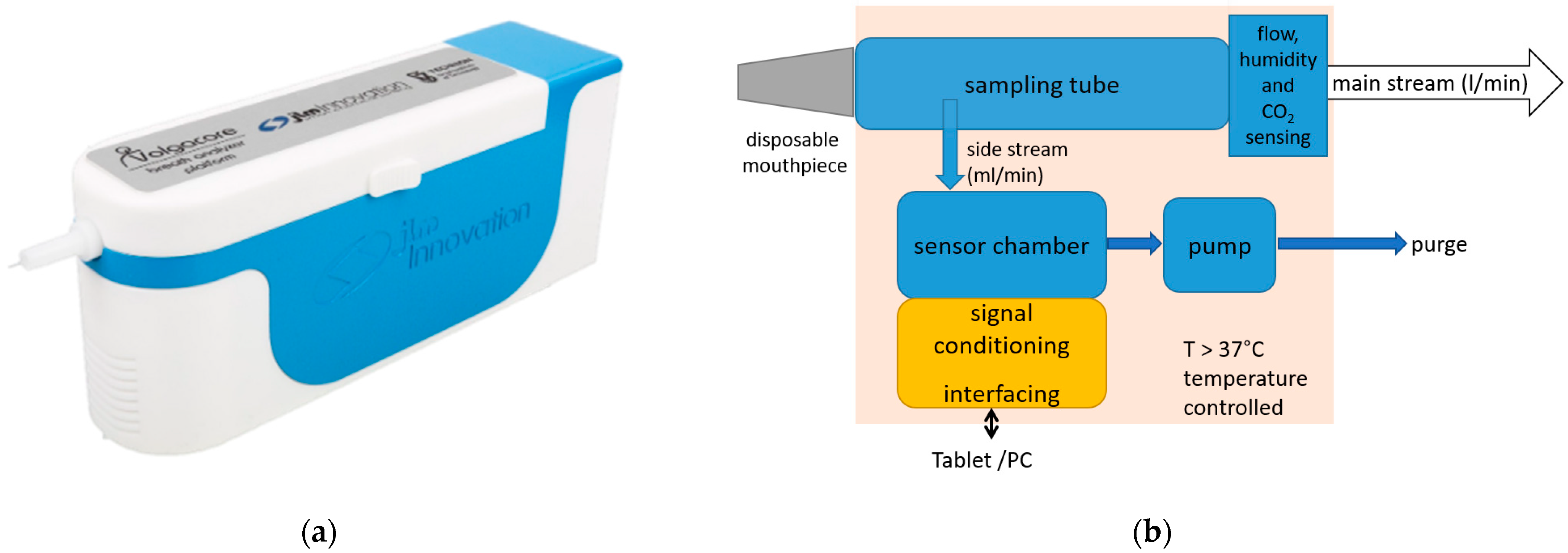
2.3. Breath Measurement
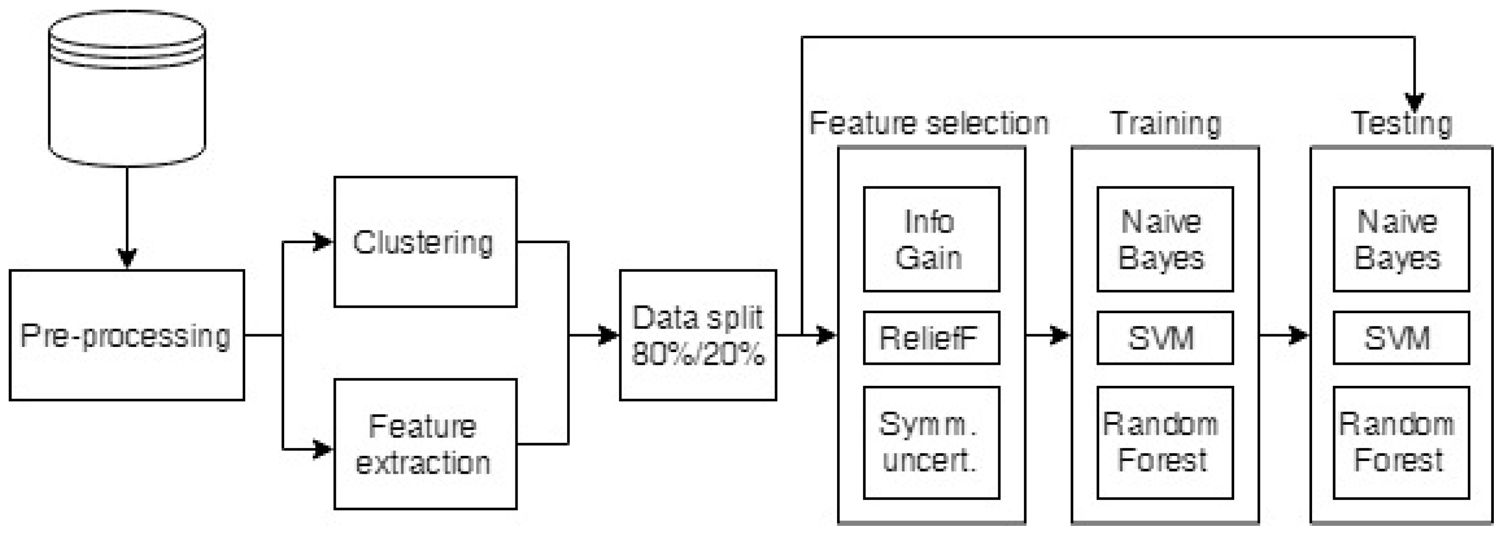
2.4. Data Analysis
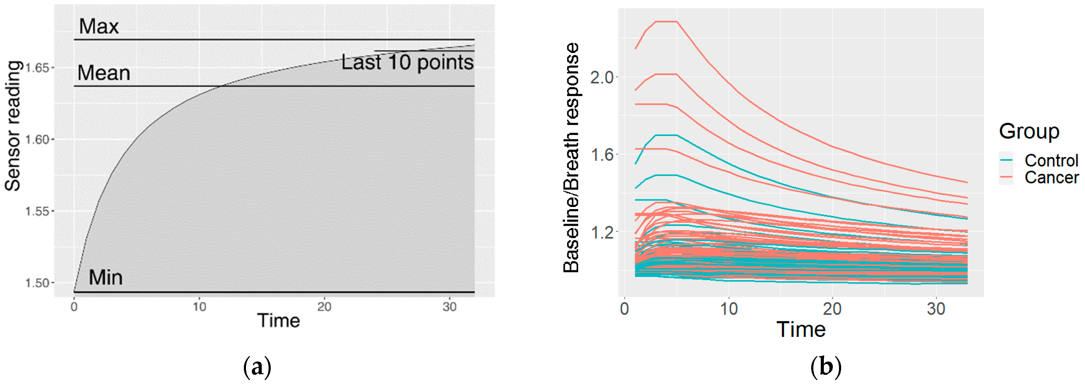
2.4.1. Preprocessing of the Raw Data
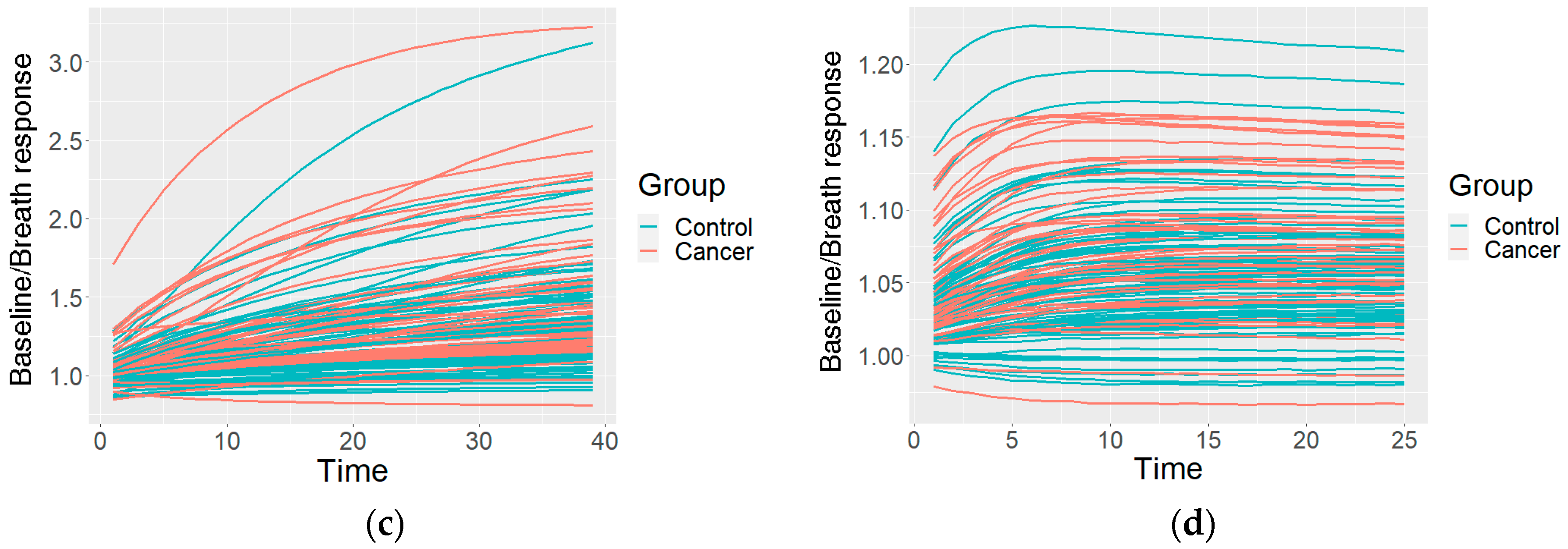
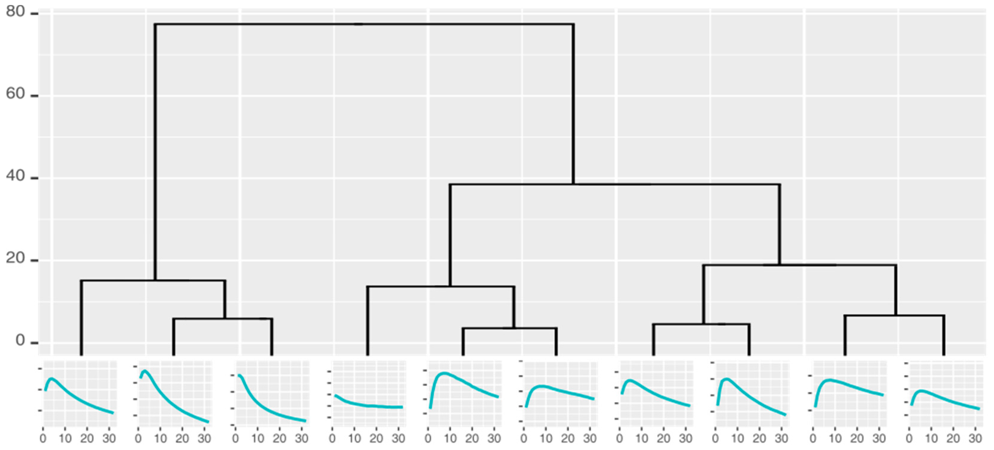
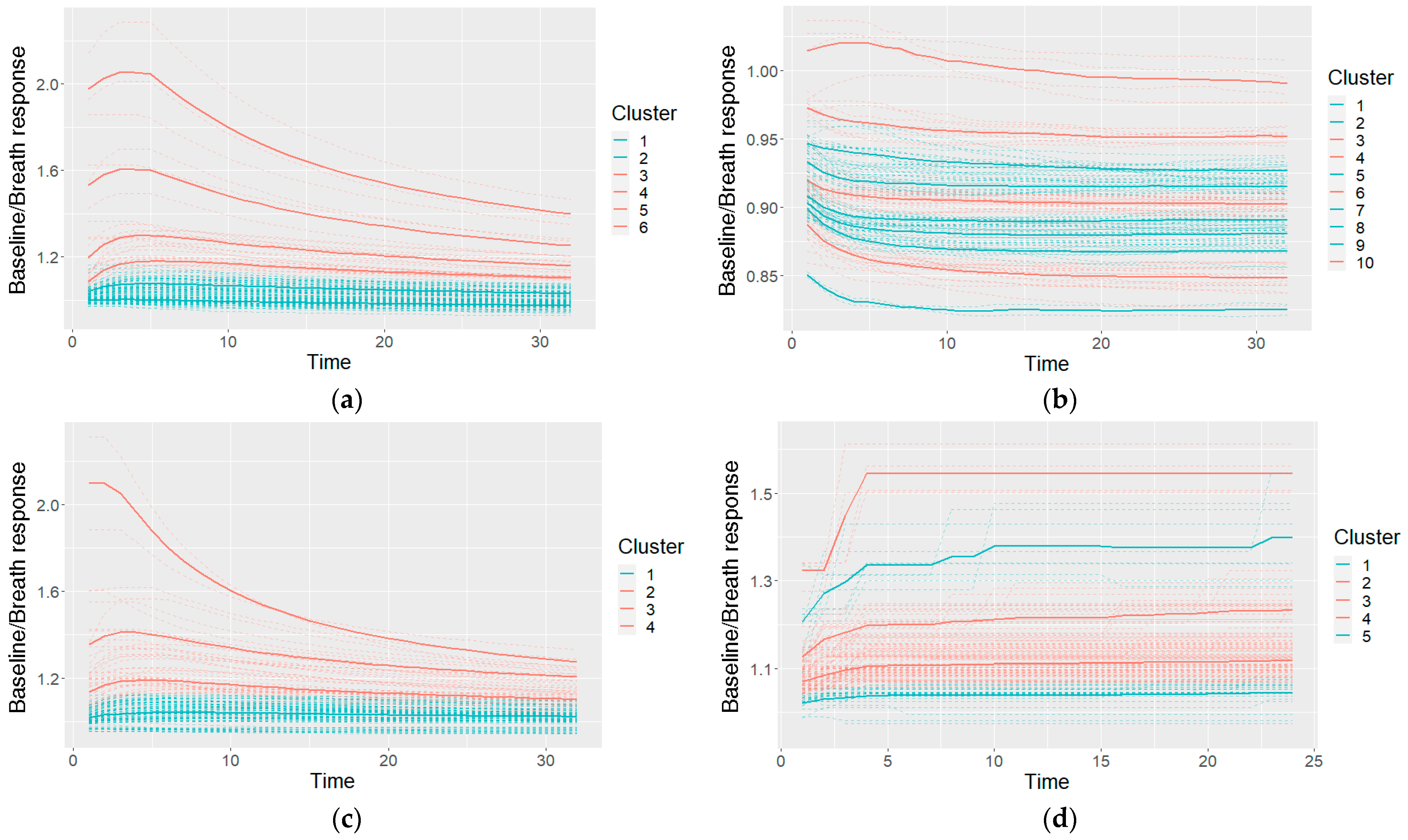
2.4.2. Clustering of the Measurements
2.4.3. Classification
3. Results
4. Discussion
5. Conclusions
Supplementary Materials
Author Contributions
Funding
Institutional Review Board Statement
Informed Consent Statement
Data Availability Statement
Conflicts of Interest
References
- Tan, Y.K.; Fielding, J.W.L. Early diagnosis of early gastric cancer. Eur. J. Gastroenterol. Hepatol. 2006, 18, 821–829. [Google Scholar] [CrossRef] [PubMed]
- Daniel, D.A.P.; Thangavel, K. Breathomics for gastric cancer classification using back-propagation neural network. J. Med. Signals Sens. 2016, 6, 172–182. [Google Scholar] [CrossRef] [PubMed]
- Amor, R.E.; Nakhleh, M.K.; Barash, O.; Haick, H. Breath analysis of cancer in the present and the future. Eur. Respir. Rev. 2019, 28, 190002. [Google Scholar] [CrossRef] [PubMed]
- Yang, H.-Y.; Chen, W.-C.; Tsai, R.-C. Accuracy of the Electronic Nose Breath Tests in Clinical Application: A Systematic Review and Meta-Analysis. Biosensors 2021, 11, 469. [Google Scholar] [CrossRef] [PubMed]
- Peng, G.; Hakim, M.; Broza, Y.Y.; Billan, S.; Abdah-Bortnyak, R.; Kuten, A.; Tisch, U.; Haick, H. Detection of lung, breast, colorectal, and prostate cancers from exhaled breath using a single array of nanosensors. Br. J. Cancer 2010, 103, 542–551. [Google Scholar] [CrossRef]
- Haddad, G.; Schouwenburg, S.; Altesha, A.; Xu, W.; Liu, G. Using breath analysis as a screening tool to detect gastric cancer: A systematic review. J. Breath Res. 2020, 175, 016013. [Google Scholar] [CrossRef]
- Amal, H.; Leja, M.; Funka, K.; Skapars, R.; Liepniece-Karele, I.; Kikuste, I.; Vanags, A.; Tolmanis, I.; Haick, H. Sa1896 Nanomaterial-Based Sensor Technology Can Detect Gastric Cancer and Peptic Ulcer Disease With a High Accuracy From an Exhaled Air Sample. Gastroenterology 2014, 146, S-323. [Google Scholar] [CrossRef]
- Miekisch, W.; Schubert, J.K.; Noeldge-Schomburg, G.F. Diagnostic potential of breath analysis—focus on volatile organic compounds. Clin. Chim. Acta 2004, 347, 25–39. [Google Scholar] [CrossRef]
- Gouzerh, F.; Bessière, J.-M.; Ujvari, B.; Thomas, F.; Dujon, A.M.; Dormont, L. Odors and cancer: Current status and future directions. Biochim. Biophys. Acta (BBA) Rev. Cancer 2021, 1877, 188644. [Google Scholar] [CrossRef]
- Zhang, J.; Tian, Y.; Luo, Z.; Qian, C.; Li, W.; Duan, Y. Breath volatile organic compound analysis: An emerging method for gastric cancer detection. J. Breath Res. 2021, 15, 044002. [Google Scholar] [CrossRef]
- Xiang, L.; Wu, S.; Hua, Q.; Bao, C.; Liu, H. Volatile Organic Compounds in Human Exhaled Breath to Diagnose Gastrointestinal Cancer: A Meta-Analysis. Front. Oncol. 2021, 11, 606915. [Google Scholar] [CrossRef] [PubMed]
- Shreffler, J.; Huecker, M.R. Diagnostic Testing Accuracy: Sensitivity, Specificity, Predictive Values and Likelihood Ratios; StatPearls Publishing: Treasure Island, FL, USA, 2020. [Google Scholar]
- Baldini, C.; Billeci, L.; Sansone, F.; Conte, R.; Domenici, C.; Tonacci, A. Electronic Nose as a Novel Method for Diagnosing Cancer: A Systematic Review. Biosensors 2020, 10, 84. [Google Scholar] [CrossRef] [PubMed]
- Bassi, P.; Di Gianfrancesco, L.; Salmaso, L.; Ragonese, M.; Palermo, G.; Sacco, E.; Giancristofaro, R.A.; Ceccato, R.; Racioppi, M. Improved Non-Invasive Diagnosis of Bladder Cancer with an Electronic Nose: A Large Pilot Study. J. Clin. Med. 2021, 10, 4984. [Google Scholar] [CrossRef] [PubMed]
- Kononov, A.; Korotetsky, B.; Jahatspanian, I.; Gubal, A.; Vasiliev, A.; Arsenjev, A.; Nefedov, A.; Barchuk, A.; Gorbunov, I.; Kozyrev, K.; et al. Online breath analysis using metal oxide semiconductor sensors (electronic nose) for diagnosis of lung cancer. J. Breath Res. 2019, 14, 016004. [Google Scholar] [CrossRef] [PubMed]
- Broza, Y.Y.; Khatib, S.; Gharra, A.; Krilaviciute, A.; Amal, H.; Polaka, I.; Parshutin, S.; Kikuste, I.; Gasenko, E.; Skapars, R.; et al. Screening for gastric cancer using exhaled breath samples. Br. J. Surg. 2019, 106, 1122–1125. [Google Scholar] [CrossRef] [PubMed]
- Xu, Z.-Q.; Broza, Y.Y.; Ionsecu, R.; Tisch, U.; Ding, L.; Liu, H.; Song, Q.; Pan, Y.-Y.; Xiong, F.-X.; Gu, K.-S.; et al. A nanomaterial-based breath test for distinguishing gastric cancer from benign gastric conditions. Br. J. Cancer 2013, 108, 941–950. [Google Scholar] [CrossRef] [Green Version]
- Su, Y.; Chen, G.; Chen, C.; Gong, Q.; Xie, G.; Yao, M.; Tai, H.; Jiang, Y.; Chen, J. Self-Powered Respiration Monitoring Enabled By a Triboelectric Nanogenerator. Adv. Mater. 2021, 33, 2101262. [Google Scholar] [CrossRef]
- Su, Y.; Wang, J.; Wang, B.; Yang, T.; Yang, B.; Xie, G.; Zhou, Y.; Zhang, S.; Tai, H.; Cai, Z.; et al. Alveolus-Inspired Active Membrane Sensors for Self-Powered Wearable Chemical Sensing and Breath Analysis. ACS Nano 2020, 14, 6067–6075. [Google Scholar] [CrossRef]
- Su, Y.; Yang, T.; Zhao, X.; Cai, Z.; Chen, G.; Yao, M.; Chen, K.; Bick, M.; Wang, J.; Li, S.; et al. A wireless energy transmission enabled wearable active acetone biosensor for non-invasive prediabetes diagnosis. Nano Energy 2020, 74, 104941. [Google Scholar] [CrossRef]
- Su, Y.; Chen, C.; Pan, H.; Yang, Y.; Chen, G.; Zhao, X.; Li, W.; Gong, Q.; Xie, G.; Zhou, Y.; et al. Muscle Fibers Inspired High-Performance Piezoelectric Textiles for Wearable Physiological Monitoring. Adv. Funct. Mater. 2021, 31, 2010962. [Google Scholar] [CrossRef]
- Wang, S.; Jiang, Y.; Tai, H.; Liu, B.; Duan, Z.; Yuan, Z.; Pan, H.; Xie, G.; Du, X.; Su, Y. An integrated flexible self-powered wearable respiration sensor. Nano Energy 2019, 63, 103829. [Google Scholar] [CrossRef]
- Wilson, A.D. Application of Electronic-Nose Technologies and VOC-Biomarkers for the Noninvasive Early Diagnosis of Gastrointestinal Diseases. Sensors 2018, 18, 2613. [Google Scholar] [CrossRef] [PubMed] [Green Version]
- Amal, H.; Leja, M.; Funka, K.; Skapars, R.; Sivins, A.; Ancans, G.; Liepniece-Karele, I.; Kikuste, I.; Lasina, I.; Haick, H. Detection of precancerous gastric lesions and gastric cancer through exhaled breath. Gut 2015, 65, 400–407. [Google Scholar] [CrossRef] [PubMed]
- Turppa, E.; Polaka, I.; Vasiljevs, E.; Kortelainen, J.M.; Shani, G.; Leja, M.; Haick, H. Repeatability Study on a Classifier for Gastric Cancer Detection from Breath Sensor Data. In Proceedings of the 2019 IEEE 19th International Conference on Bioinformatics and Bioengineering (BIBE), Athens, Greece, 28–30 October 2019; pp. 450–453. [Google Scholar] [CrossRef]
- Leja, M.; Kortelainen, J.M.; Polaka, I.; Turppa, E.; Mitrovics, J.; Padilla, M.; Mochalski, P.; Shuster, G.; Pohle, R.; Kashanin, D.; et al. Sensing gastric cancer via point-of-care sensor breath analyzer. Cancer 2021, 127, 1286–1292. [Google Scholar] [CrossRef]
- Rodionova, O.Y.; Pomerantsev, A.L. Detection of Outliers in Projection-Based Modeling. Anal. Chem. 2019, 92, 2656–2664. [Google Scholar] [CrossRef]
- Scott, S.; James, D.; Ali, Z. Data analysis for electronic nose systems. Mikrochim. Acta 2006, 156, 183–207. [Google Scholar] [CrossRef]
- Yan, J.; Guo, X.; Duan, S.; Jia, P.; Wang, L.; Peng, C.; Zhang, S. Electronic Nose Feature Extraction Methods: A Review. Sensors 2015, 15, 27804–27831. [Google Scholar] [CrossRef]
- Berndt, D.; Clifford, J. Using dynamic time warping to find patterns in time series. KDD Workshop 1994, 10, 359–370. [Google Scholar] [CrossRef]
- Wang, X.; Mueen, A.; Ding, H.; Trajcevski, G.; Scheuermann, P.; Keogh, E. Experimental comparison of representation methods and distance measures for time series data. Data Min. Knowl. Discov. 2012, 26, 275–309. [Google Scholar] [CrossRef] [Green Version]
- Johnpaul, C.I.; Prasad, M.V.; Nickolas, S.; Gangadharan, G.R. A novel probabilistic representational structures for clustering the time series data. Expert Syst. Appl. 2020, 145, 113119. [Google Scholar] [CrossRef]
- Kullback, S.; Leibler, R.A. On Information and Sufficiency. Ann. Math. Stat. 1951, 22, 79–86. [Google Scholar] [CrossRef]
- Kononenko, I.; Šimec, E.; Robnik-Šikonja, M. Overcoming the Myopia of Inductive Learning Algorithms with RELIEFF. Appl. Intell. 1997, 7, 39–55. [Google Scholar] [CrossRef]
- Robnik-Šikonja, M.; Kononenko, I. Theoretical and Empirical Analysis of ReliefF and RReliefF. Mach. Learn. 2003, 53, 23–69. [Google Scholar] [CrossRef] [Green Version]
- Yu, L.; Liu, H. Feature selection for high-dimensional data: A fast correlation-based filter solution. In Proceedings of the Twentieth International Conference on Machine Learning (ICML-2003), Washington, DC, USA, 21–24 August 2003; pp. 856–863. [Google Scholar]
- Frank, E.; Hall, M.A.; Witten, I.H. The WEKA Workbench. Online Appendix. In Data Mining: Practical Machine Learning Tools and Techniques, 4th ed.; Morgan Kaufmann Publishers Inc.: Burlington, MA, USA, 2016. [Google Scholar]
- John, G.H.; Langley, P. Estimating Continuous Distributions in Bayesian Classifiers. In UAI’ 95: Proceedings of the Eleventh Conference on Uncertainty in Artificial Intelligence, 1995; Morgan Kaufmann Publishers Inc.: Montréal, QC, Canada; pp. 338–345. [CrossRef]
- Keerthi, S.S.; Shevade, S.K.; Bhattacharyya, C.; Murthy, K.R.K. Improvements to Platt’s SMO Algorithm for SVM Classifier Design. Neural Comput. 2001, 13, 637–649. [Google Scholar] [CrossRef]
- Breiman, L. Random forests. Mach. Learn. 2001, 45, 5–32. [Google Scholar] [CrossRef] [Green Version]
- Karakaya, D.; Ulucan, O.; Turkan, M. Electronic Nose and Its Applications: A Survey. Int. J. Autom. Comput. 2019, 17, 179–209. [Google Scholar] [CrossRef] [Green Version]
- Chen, Y.; Zhang, Y.; Pan, F.; Liu, J.; Wang, K.; Zhang, C.; Cheng, S.; Lu, L.; Zhang, W.; Zhang, Z.; et al. Breath Analysis Based on Surface-Enhanced Raman Scattering Sensors Distinguishes Early and Advanced Gastric Cancer Patients from Healthy Persons. ACS Nano 2016, 10, 8169–8179. [Google Scholar] [CrossRef]
- Gharra, A.; Broza, Y.Y.; Yu, G.; Mao, W.; Shen, D.; Deng, L.; Wu, C.; Wang, Q.; Sun, X.; Huang, J.; et al. Exhaled breath diagnostics of lung and gastric cancers in China using nanosensors. Cancer Commun. 2020, 40, 273–278. [Google Scholar] [CrossRef]
- Nakhleh, M.K.; Amal, H.; Jeries, R.; Broza, Y.Y.; Aboud, M.; Gharra, A.; Ivgi, H.; Khatib, S.; Badarneh, S.; Har-Shai, L.; et al. Diagnosis and Classification of 17 Diseases from 1404 Subjects via Pattern Analysis of Exhaled Molecules. ACS Nano 2017, 11, 112–125. [Google Scholar] [CrossRef] [Green Version]
- Aslam, M.A.; Xue, C.; Chen, Y.; Zhang, A.; Liu, M.; Wang, K.; Cui, D. Breath analysis based early gastric cancer classification from deep stacked sparse autoencoder neural network. Sci. Rep. 2021, 11, 4014. [Google Scholar] [CrossRef]
- Kim, C.; Raja, I.S.; Lee, J.-M.; Lee, J.H.; Kang, M.S.; Lee, S.H.; Oh, J.-W.; Han, D.-W. Recent Trends in Exhaled Breath Diagnosis Using an Artificial Olfactory System. Biosensors 2021, 11, 337. [Google Scholar] [CrossRef] [PubMed]
- Schuermans, V.N.E.; Li, Z.; Jongen, A.C.H.M.; Wu, Z.; Shi, J.; Ji, J.; Bouvy, N.D. Pilot Study: Detection of Gastric Cancer from Exhaled Air Analyzed with an Electronic Nose in Chinese Patients. Surg. Innov. 2018, 25, 429–434. [Google Scholar] [CrossRef] [PubMed]
- Durán-Acevedo, C.M.; Jaimes-Mogollón, A.L.; Gualdrón-Guerrero, O.E.; Welearegay, T.G.; Martinez-Marín, J.D.; Caceres-Tarazona, J.M.; Acevedo, Z.C.S.; Beleño-Saenz, K.D.J.; Cindemir, U.; Österlund, L.; et al. Exhaled breath analysis for gastric cancer diagnosis in Colombian patients. Oncotarget 2018, 9, 28805–28817. [Google Scholar] [CrossRef] [PubMed]


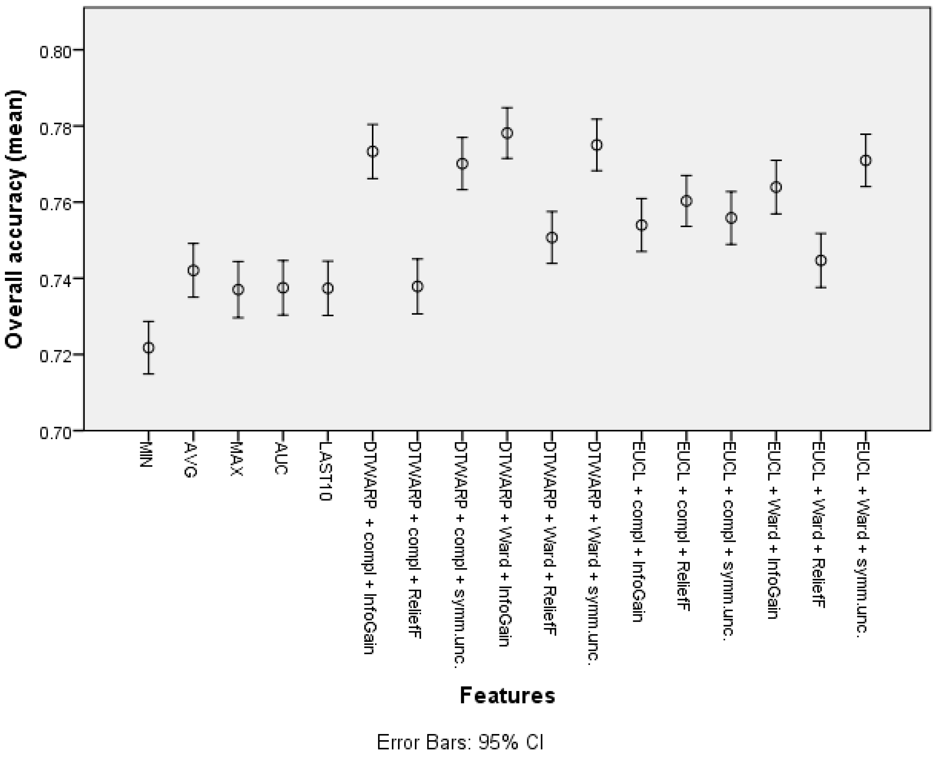
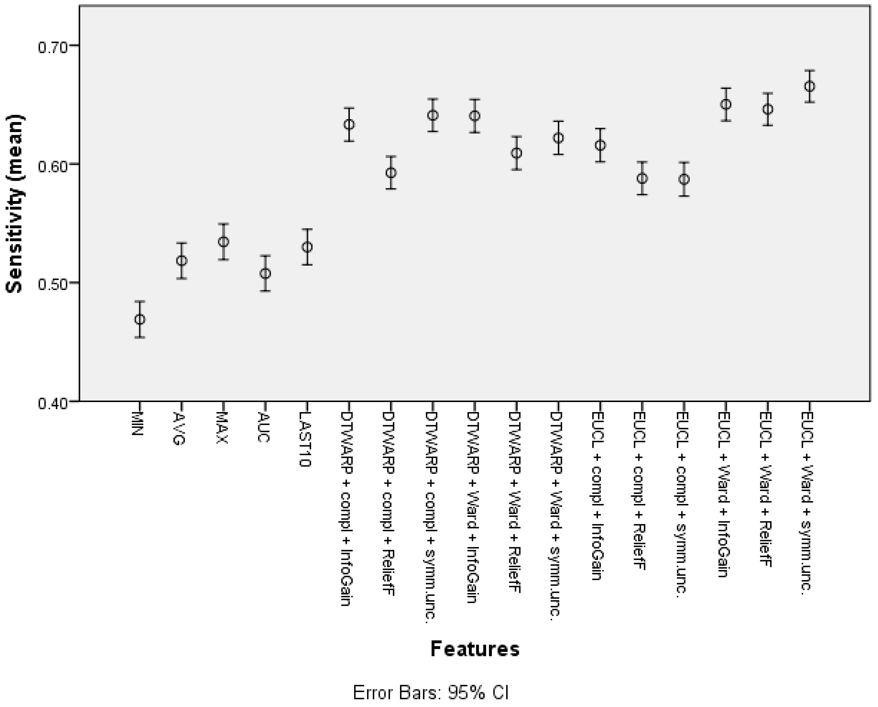
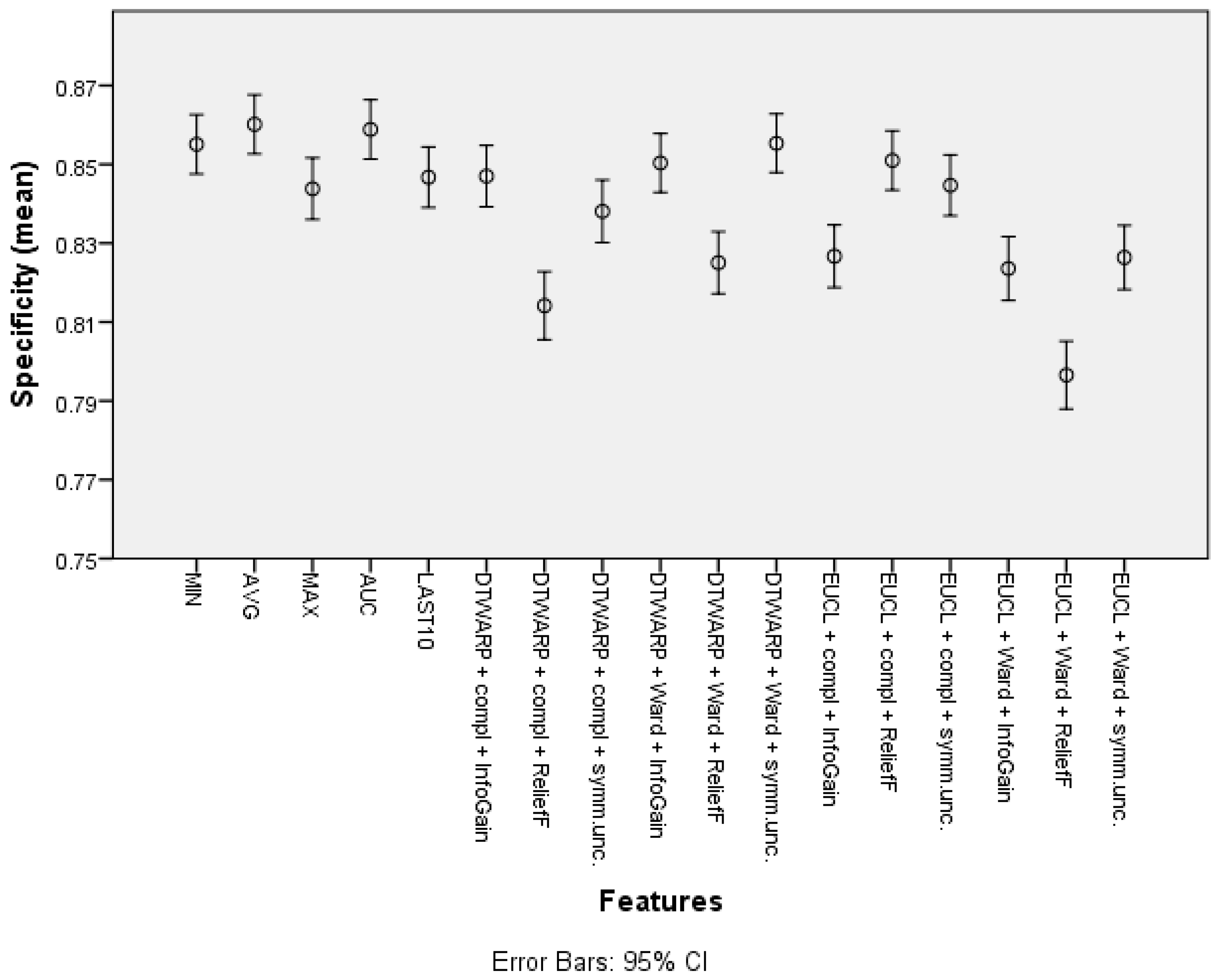
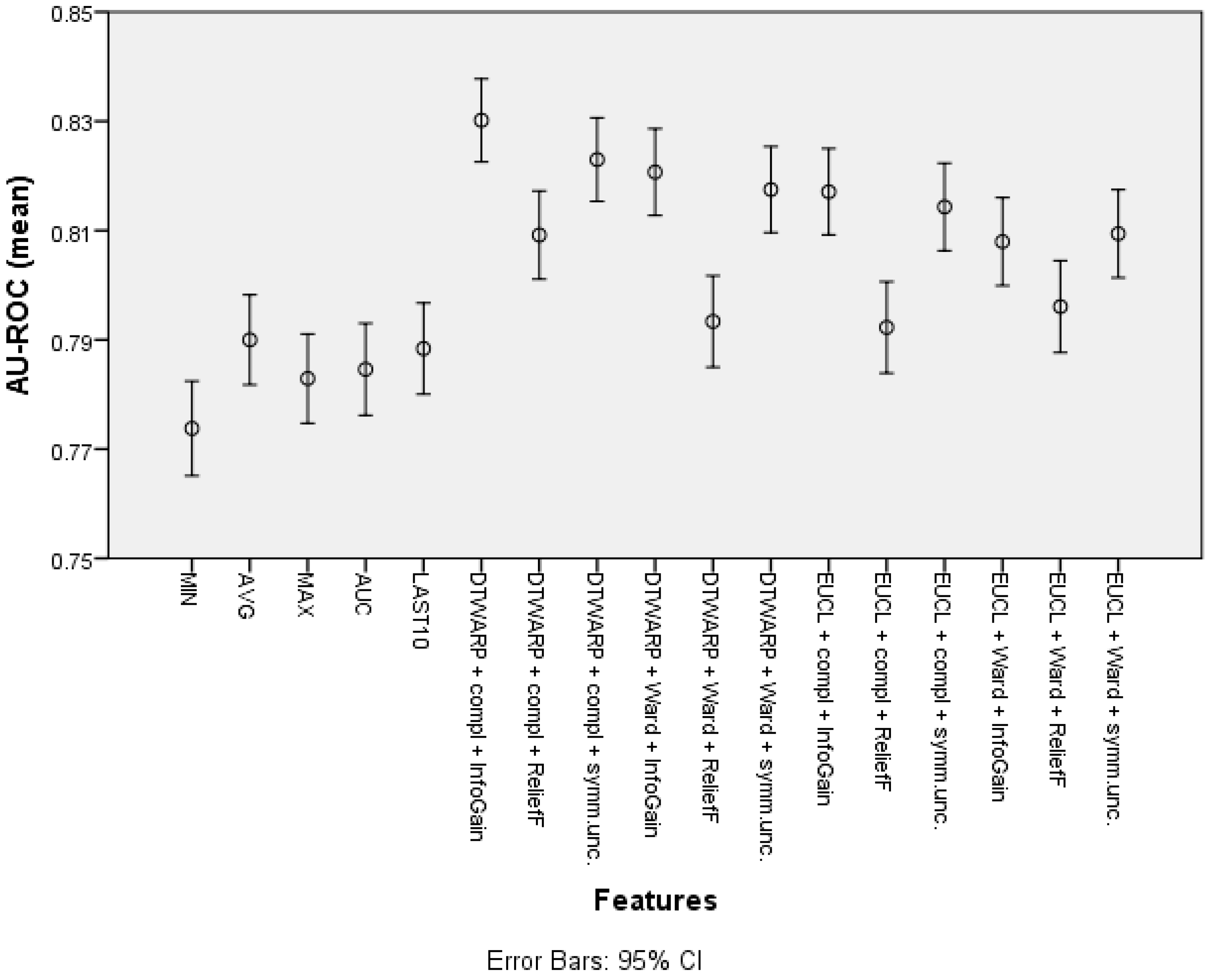
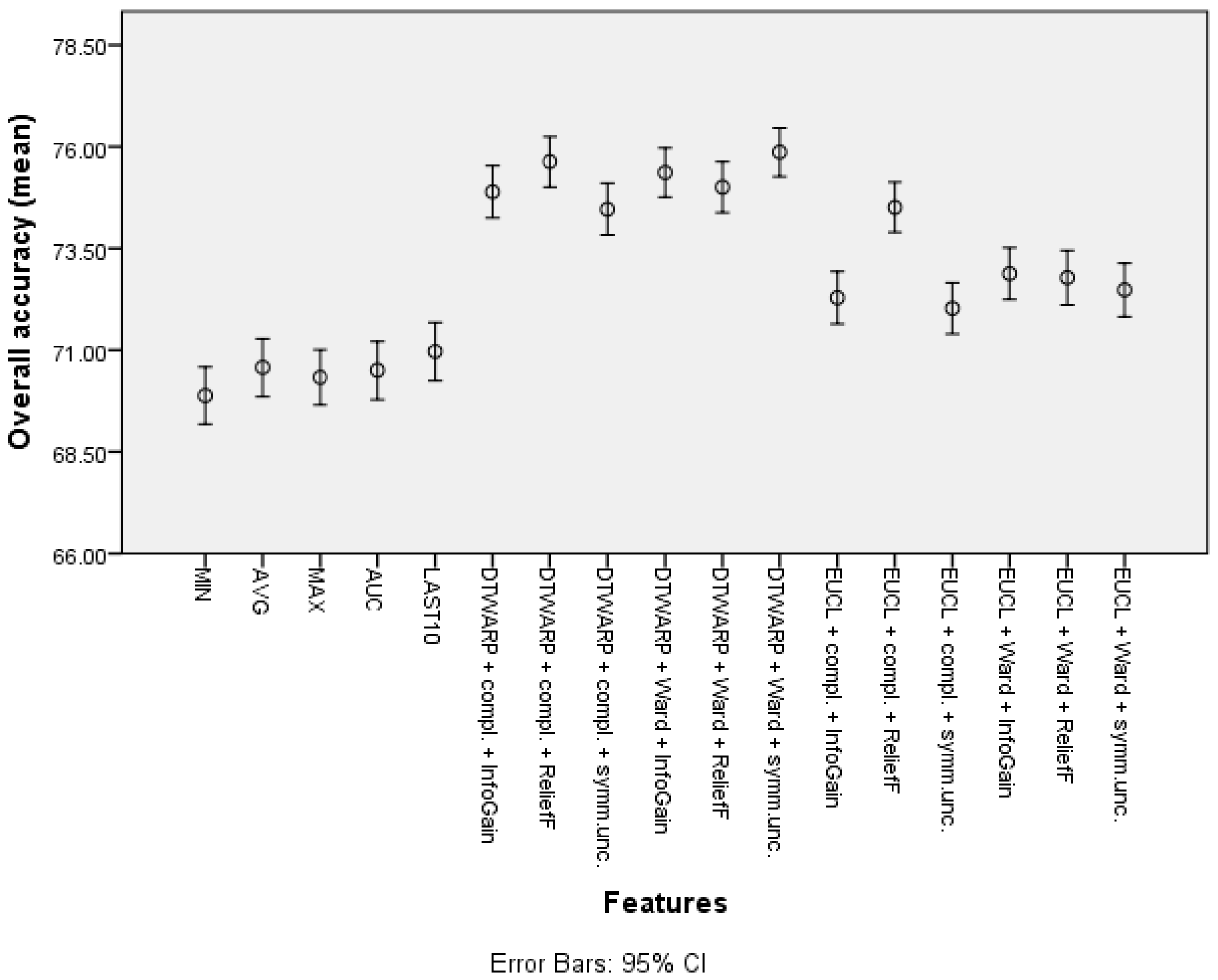
| Feature | Overall Accuracy | Sensitivity | Specificity |
|---|---|---|---|
| Minimum | 72.18% (71.49–72.87%) | 46.9% (45.39–48.41%) | 85.51% (84.76–86.26%) |
| Average | 74.21% (73.5–74.91%) | 51.85% (50.35–53.34%) | 86.02% (85.27–86.76%) |
| Maximum | 73.7% (72.96–74.44%) | 53.44% (51.94–54.94%) | 84.38% (83.6–85.16%) |
| Average of the last 10 time points | 73.74% (73.02–74.45%) | 53.00% (51.51–54.49%) | 84.67% (83.9–85.44%) |
| Area under the curve | 73.75% (73.04–74.47%) | 50.77% (49.28–52.26%) | 85.88% (85.13–86.64%) |
| Cluster (DTWARP distance, Ward linkage, InfoGain) | 77.81% (77.15–78.48%) | 64.05% (62.66–65.44%) | 85.04% (84.29–85.78%) |
| Cluster (Euclidean distance, Ward linkage, Symm.Unc.) | 77.1% (76.41–77.79%) | 66.54% (65.21–67.87%) | 82.64% (81.83–83.45%) |
| Feature | Overall Accuracy | Sensitivity | Specificity |
|---|---|---|---|
| Minimum | 69.89% (69.19–70.59%) | 45.3% (43.87–46.73%) | 82.93% (82.12–83.74%) |
| Average | 70.58% (69.86–71.29%) | 47% (45.56–48.45%) | 83.13% (82.3–83.95%) |
| Maximum | 70.33% (69.66–71.01%) | 43.23% (41.82–44.64%) | 84.72% (83.95–85.49%) |
| Average of the last 10 time points | 70.97% (70.25–71.69%) | 48.79% (47.32–50.25%) | 82.78% (81.96–83.6%) |
| Area under the curve | 70.51% (69.79–71.23%) | 46.54% (45.1–47.99%) | 83.27% (82.44–84.1%) |
| Cluster (DTWARP distance, Ward linkage, ReliefF) | 75.01% (74.39–75.63%) | 46.52% (45.13–47.91%) | 90.12% (89.5–90.74%) |
| Cluster (Euclidean distance, complete linkage, ReliefF) | 74.51% (73.90–75.13%) | 46.04% (44.68–47.41%) | 89.66% (89.01–90.30%) |
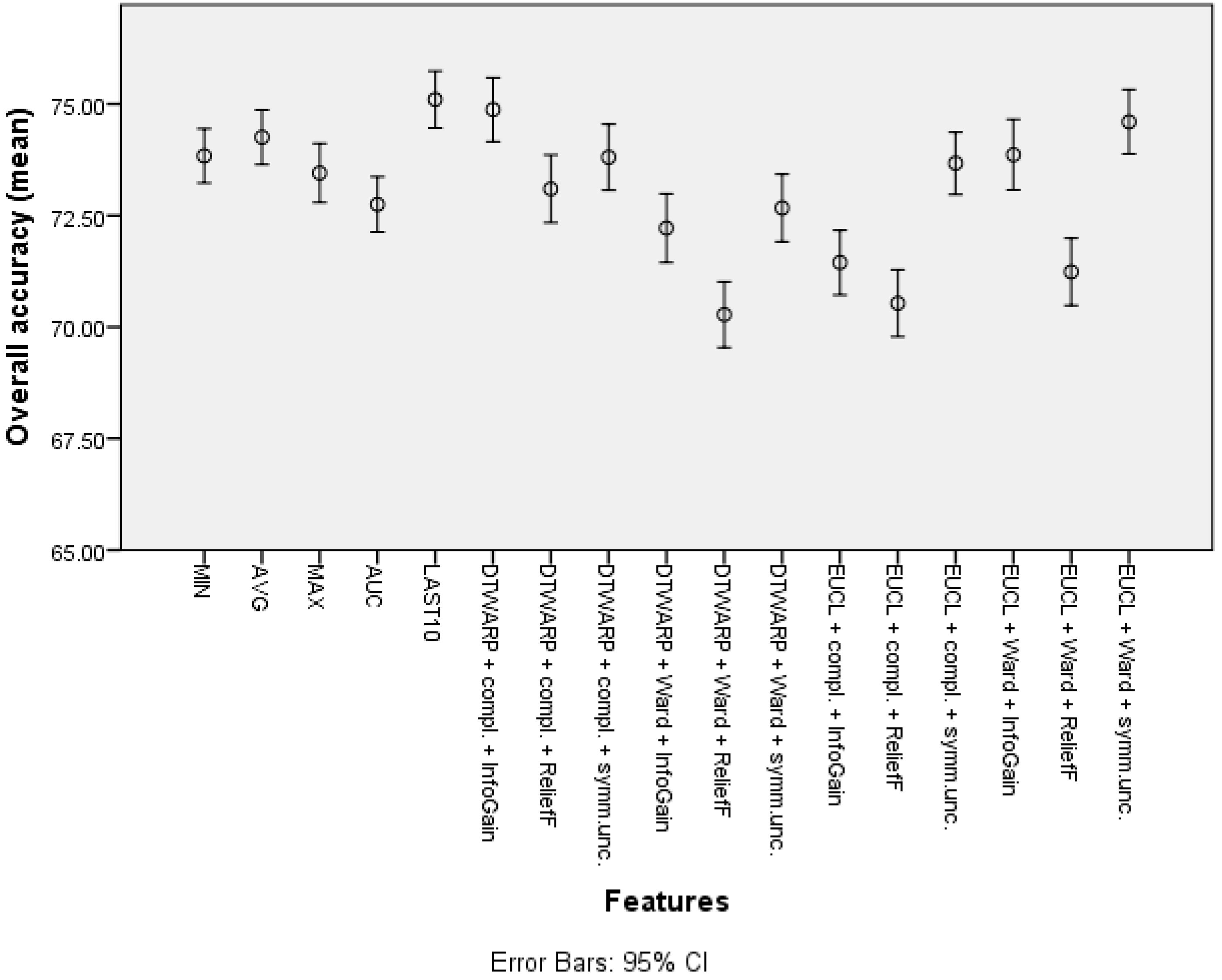
| Feature | Overall Accuracy | Sensitivity | Specificity |
|---|---|---|---|
| Minimum | 73.84% (73.23–74.45%) | 41.31% (39.99–42.64%) | 91.14% (90.51–91.78%) |
| Maximum | 73.45% (72.79–74.11%) | 45.72% (44.31–47.14%) | 88.2% (87.53–88.88%) |
| Average | 74.26% (73.64–74.87%) | 43.16% (41.77–44.55%) | 90.74% (90.12–91.37%) |
| Average of the last 10 time points | 75.1% (74.47–75.74%) | 48.33% (46.94–49.71%) | 89.27% (88.62–89.92%) |
| Area under the curve | 72.75% (72.13–73.37%) | 40.86% (39.48–42.25%) | 89.68% (89.02–90.33%) |
| Cluster (DTWARP distance, complete linkage, InfoGain) | 74.87% (74.16–75.59%) | 60.73% (59.31–62.15%) | 82.48% (81.66–83.30%) |
| Cluster (Euclidean distance, Ward linkage, InfoGain) | 73.86% (73.07–74.65%) | 61.05% (59.52–62.58%) | 80.72% (79.84–81.6%) |
Publisher’s Note: MDPI stays neutral with regard to jurisdictional claims in published maps and institutional affiliations. |
© 2022 by the authors. Licensee MDPI, Basel, Switzerland. This article is an open access article distributed under the terms and conditions of the Creative Commons Attribution (CC BY) license (https://creativecommons.org/licenses/by/4.0/).
Share and Cite
Polaka, I.; Bhandari, M.P.; Mezmale, L.; Anarkulova, L.; Veliks, V.; Sivins, A.; Lescinska, A.M.; Tolmanis, I.; Vilkoite, I.; Ivanovs, I.; et al. Modular Point-of-Care Breath Analyzer and Shape Taxonomy-Based Machine Learning for Gastric Cancer Detection. Diagnostics 2022, 12, 491. https://doi.org/10.3390/diagnostics12020491
Polaka I, Bhandari MP, Mezmale L, Anarkulova L, Veliks V, Sivins A, Lescinska AM, Tolmanis I, Vilkoite I, Ivanovs I, et al. Modular Point-of-Care Breath Analyzer and Shape Taxonomy-Based Machine Learning for Gastric Cancer Detection. Diagnostics. 2022; 12(2):491. https://doi.org/10.3390/diagnostics12020491
Chicago/Turabian StylePolaka, Inese, Manohar Prasad Bhandari, Linda Mezmale, Linda Anarkulova, Viktors Veliks, Armands Sivins, Anna Marija Lescinska, Ivars Tolmanis, Ilona Vilkoite, Igors Ivanovs, and et al. 2022. "Modular Point-of-Care Breath Analyzer and Shape Taxonomy-Based Machine Learning for Gastric Cancer Detection" Diagnostics 12, no. 2: 491. https://doi.org/10.3390/diagnostics12020491