
Review of Semantic Segmentation of Medical Images Using Modified Architectures of UNET

Abstract
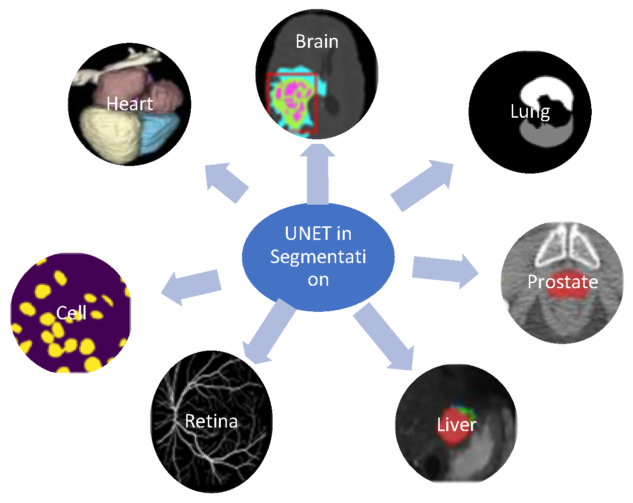
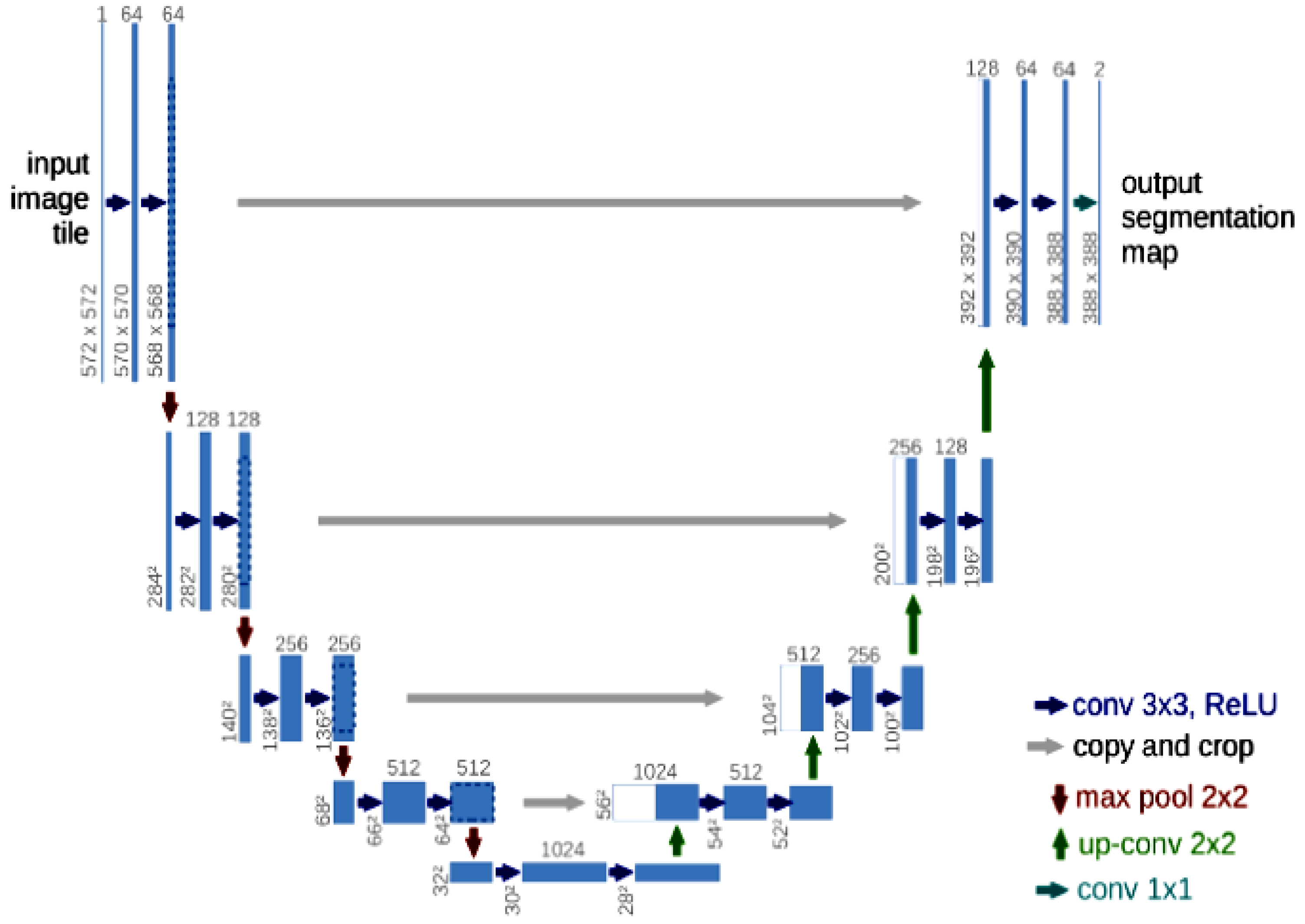
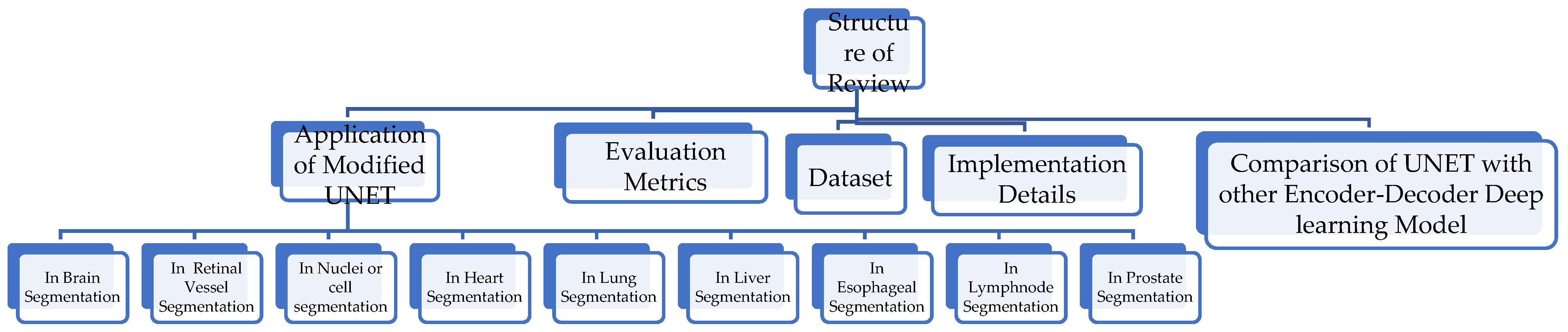
:1. Introduction
![Diagnostics 12 03064 i001]()
- In-depth review of UNET-modified architectures;
![Diagnostics 12 03064 i001]()
- Benchmark datasets and semantic architectures specifically designed for medical image segmentation;
![Diagnostics 12 03064 i001]()
- Presents the application of modified architectures of UNET in the segmentation of anatomical structures and a lesion in different organs to diagnose diseases;
![Diagnostics 12 03064 i001]()
- An updated survey of the improvement mechanisms, latest techniques, evaluation metrics, and challenges.

2. Study Method
3. Application of Modified UNET
3.1. InBrain Segmentation
3.1.1. UNET with Generalized Pooling
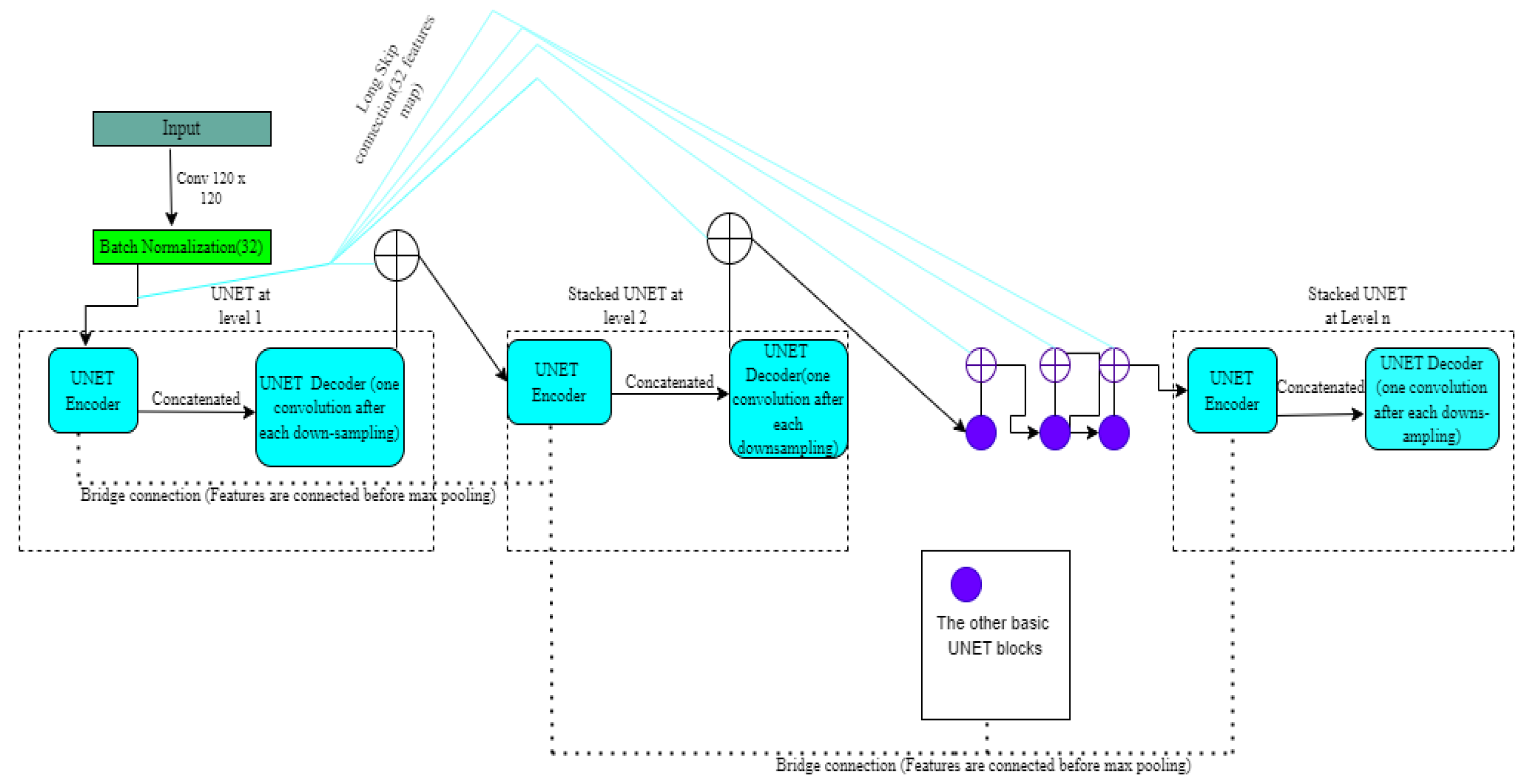
3.1.2. Stack Multi-Connection Simple Reducing Net (SMCSRNET)
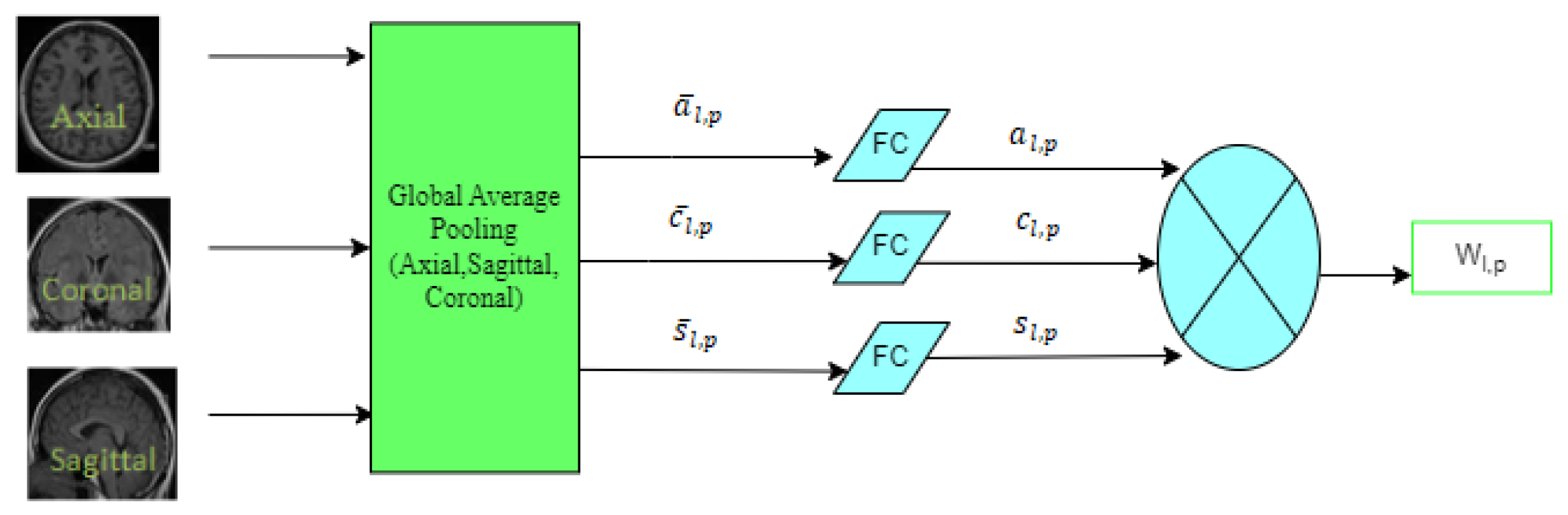
3.1.3. 3D Spatial Weighted UNET
3.1.4. Anatomical Guided UNET
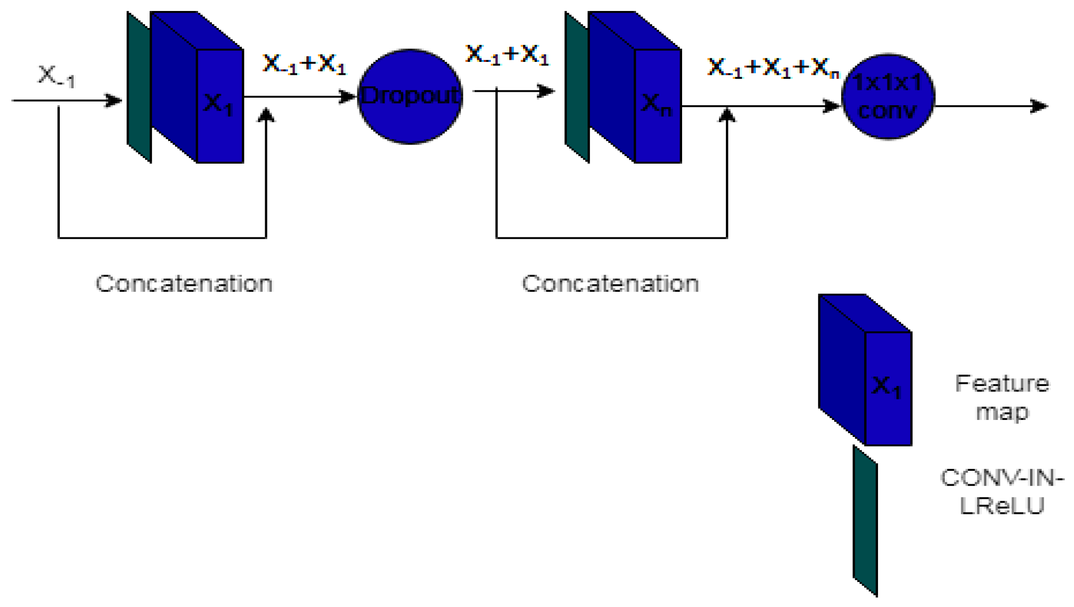
3.1.5. MH-UNET
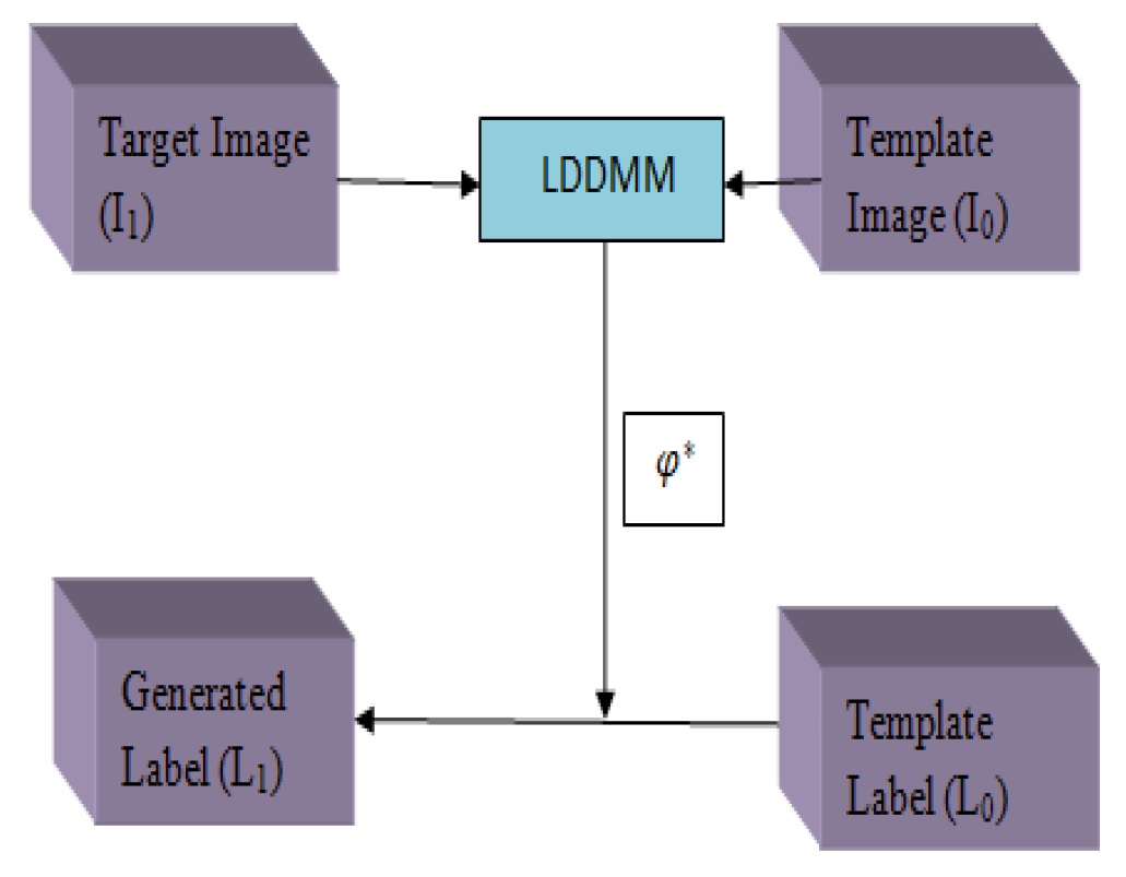
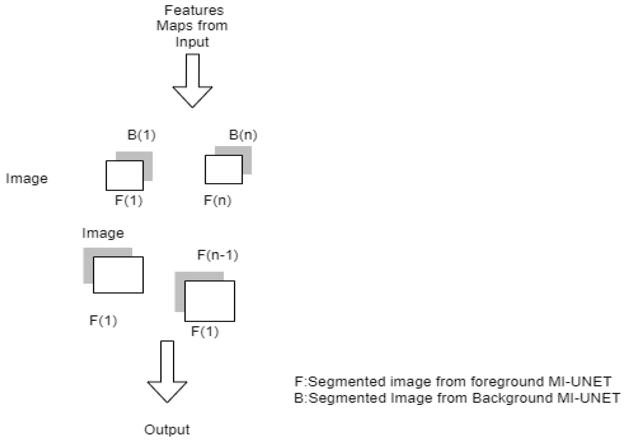
3.1.6. MI-UNET
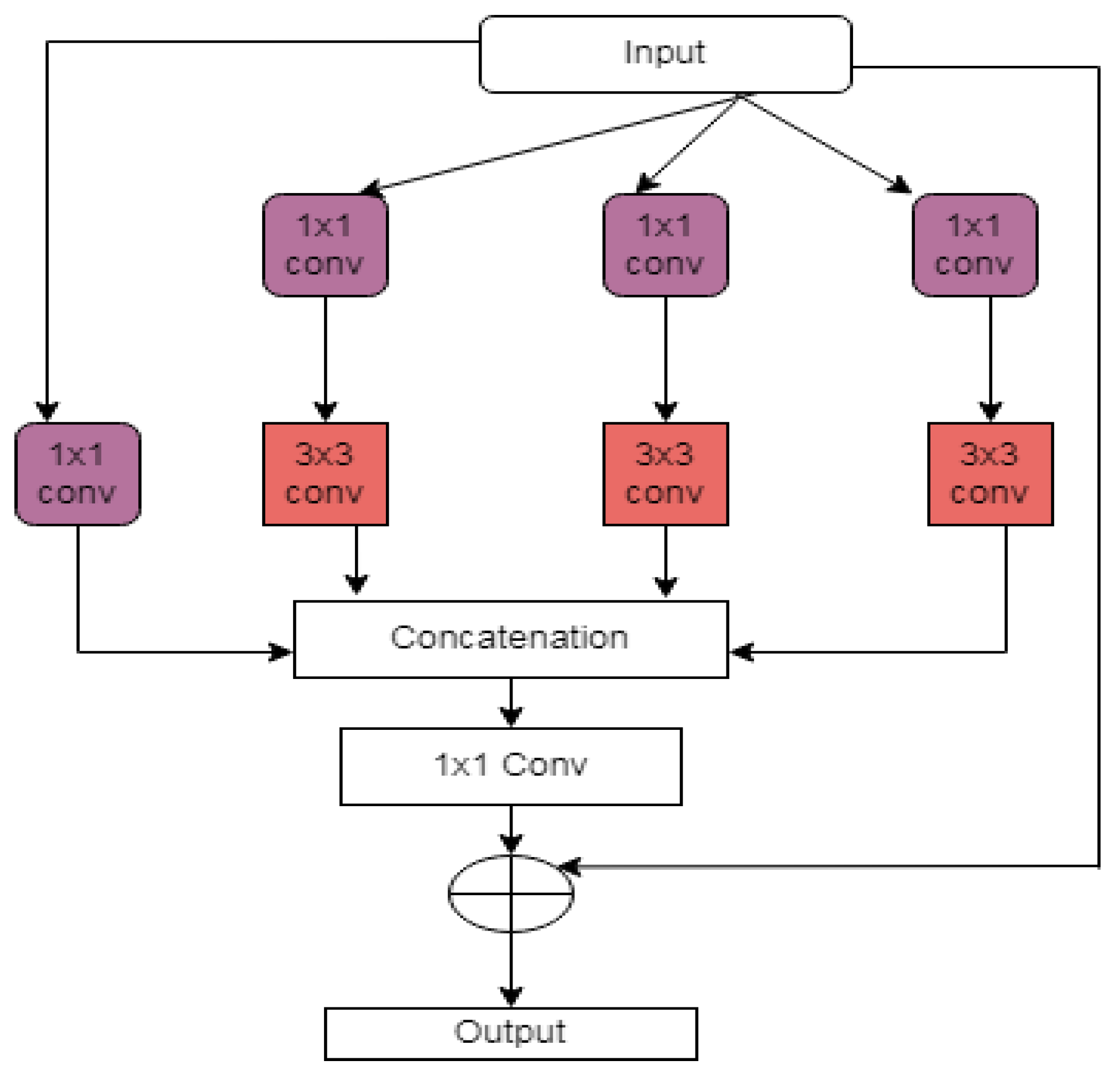
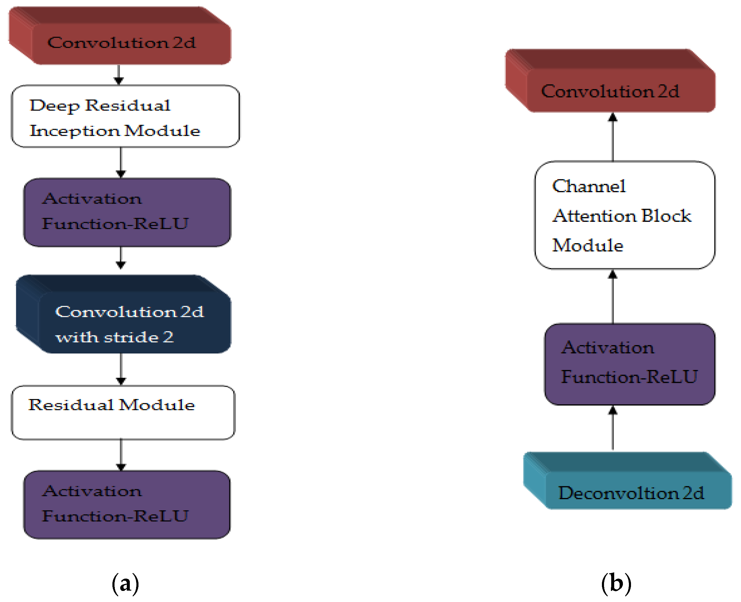
3.1.7. Multi-Res Attention UNET
3.2. In Retinal Vessel Segmentation
3.2.1. GLUE [29]
3.2.2. S-UNET
3.3. In Nuclei or Cell Segmentation
3.3.1. As-Unet
3.3.2. RIC-UNET
3.4. UNET in Heart CT Segmentation
3.4.1. Modified 2D UNET
3.4.2. UCNET with Attention Mechanism
3.5. UNET in Lung Segmentation
3.5.1. Cascaded UNET [36]
3.5.2. Res-D-UNET
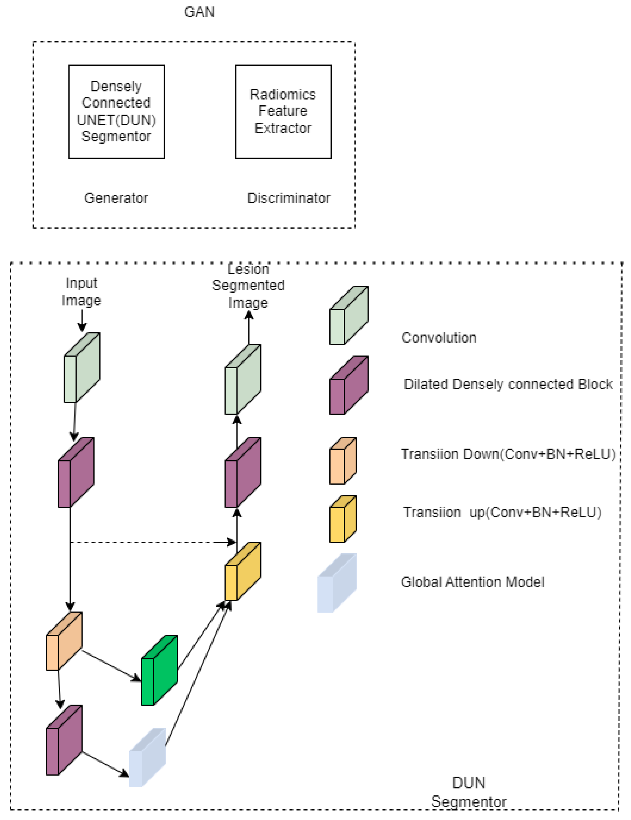
3.6. UNET in Liver Segmentation
3.7. UNET in Esophageal Segmentation
3.8. UNET in Lymphnodes Segmentation
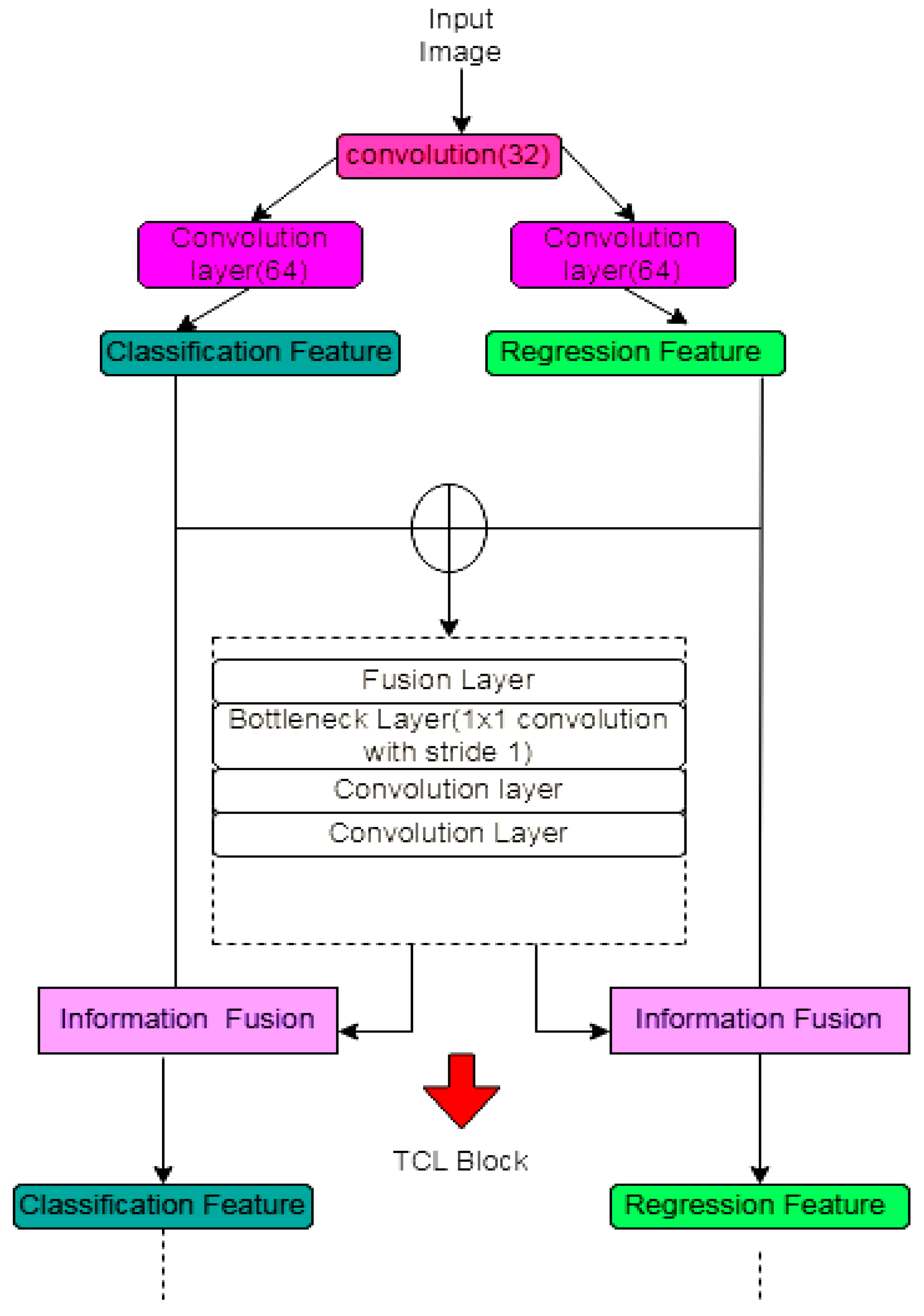
3.9. UNET in Prostate Segmentation
4. Evaluation Metrics
- DSC
- PPV–positive predictive value or precision
- Accuracy
- Sensitivity or recall
- F1 score
- AUC (area under curve) [56]
- The 95th percentile Hausdroff distance
- Absolute volume difference
- Jaccard score or IOU [59]
- Matthews correlation coefficients (MCC) [60]
5. Datasets
5.1. MRBrainS18 [61,62]
5.2. IBRS
5.3. BRATS
5.4. ADNI
5.5. ATLAS
5.6. CHASE_DB1
5.7. DRIVE
5.8. STARE [71]
5.9. RITE [72,73]
5.10. CCAP IEEE Data Port [74]
5.11. SARS-CoV-2 CT-Scan Dataset [75]
5.12. CHAOS [76]
5.13. ISLES [77]
5.14. TCGA [78]
5.15. MOD [79]
5.16. BNS [80]
5.17. Medical Segmentation Decathlon (MSD) [81]
6. Implementation Details
- Deep learning primitives are pre-built building blocks that can be used to define training elements such as tensor transformations, activation functions, and convolutions;
- Deep learning inference engine, a runtime you may use to deploy models in real-world settings;
- GPU-accelerated transcoding and inference are made possible by deep learning for video analytics, which also offers a high-level C++ runtime and API;
- Linear algebra—uses GPU acceleration to provide functionality for BLAS (basic linear algebra subprograms). Compared to the CPU this is 6–17 times faster;
- Sparse matrix operations let to use of GPU-accelerated BLAS with sparse matrices, such asthose required for natural language processing (NLP);
- Multi-GPU communication—allows for group communications over up to eight GPUs, including broadcast, reduction, and all-gather.
7. Comparison of UNET with Other Encoder–Decoder Deep Learning Model
8. Discussion
9. Conclusions and Future Work
Author Contributions
Funding
Institutional Review Board Statement
Informed Consent Statement
Data Availability Statement
Conflicts of Interest
References
- Li, B.N.; Wang, X.; Wang, R.; Zhou, T.; Gao, R.; Ciaccio, E.J.; Green, P.H. Celiac Disease Detection from Videocapsule Endoscopy Images Using Strip Principal Component Analysis. IEEE/ACM Trans. Comput. Biol. Bioinform. 2021, 18, 1396–1404. [Google Scholar] [CrossRef] [PubMed]
- Chang, H.-H.; Hsieh, C.-C. Brain segmentation in MR images using a texture-based classifier associated with mathematical morphology. In Proceedings of the 2017 39th Annual International Conference of the IEEE Engineering in Medicine and Biology Society (EMBC), Jeju Island, Republic of Korea, 11–15 July 2017; pp. 3421–3424. [Google Scholar] [CrossRef]
- Venkatachalam, K.; Siuly, S.; Bacanin, N.; Hubalovsky, S.; Trojovsky, P. An Efficient Gabor Walsh-Hadamard Transform Based Approach for Retrieving Brain Tumor Images from MRI. IEEE Access 2021, 9, 119078–119089. [Google Scholar] [CrossRef]
- Haghighi, S.J.; Komeili, M.; Hatzinakos, D.; El Beheiry, H. 40-Hz ASSR for Measuring Depth of Anaesthesia During Induction Phase. IEEE J. Biomed. Health Inform. 2018, 22, 1871–1882. [Google Scholar] [CrossRef] [PubMed]
- Tang, C.; Yu, C.; Gao, Y.; Chen, J.; Yang, J.; Lang, J.; Liu, C.; Zhong, L.; He, Z.; Lv, J. Deep learning in the nuclear industry: A survey. Big Data Min. Anal. 2022, 5, 140–160. [Google Scholar] [CrossRef]
- Jalali, S.M.J.; Osorio, G.J.; Ahmadian, S.; Lotfi, M.; Campos, V.M.A.; Shafie-Khah, M.; Khosravi, A.; Catalao, J.P.S. New Hybrid Deep Neural Architectural Search-Based Ensemble Reinforcement Learning Strategy for Wind Power Forecasting. IEEE Trans. Ind. Appl. 2022, 58, 15–27. [Google Scholar] [CrossRef]
- Tran, M.-Q.; Elsisi, M.; Liu, M.-K.; Vu, V.Q.; Mahmoud, K.; Darwish, M.M.F.; Abdelaziz, A.Y.; Lehtonen, M. Reliable Deep Learning and IoT-Based Monitoring System for Secure Computer Numerical Control Machines Against Cyber-Attacks with Experimental Verification. IEEE Access 2022, 10, 23186–23197. [Google Scholar] [CrossRef]
- Cao, Q.; Zhang, W.; Zhu, Y. Deep learning-based classification of the polar emotions of “moe”-style cartoon pictures. Tsinghua Sci. Technol. 2021, 26, 275–286. [Google Scholar] [CrossRef]
- Liu, S.; Xia, Y.; Shi, Z.; Yu, H.; Li, Z.; Lin, J. Deep Learning in Sheet Metal Bending with a Novel Theory-Guided Deep Neural Network. IEEE/CAA J. Autom. Sin. 2021, 8, 565–581. [Google Scholar] [CrossRef]
- Monteiro, N.R.C.; Ribeiro, B.; Arrais, J.P. Drug-Target Interaction Prediction: End-to-End Deep Learning Approach. IEEE/ACM Trans. Comput. Biol. Bioinform. 2020, 18, 2364–2374. [Google Scholar] [CrossRef]
- Mohsen, S.; Elkaseer, A.; Scholz, S.G. Industry 4.0-Oriented Deep Learning Models for Human Activity Recognition. IEEE Access 2021, 9, 150508–150521. [Google Scholar] [CrossRef]
- Lee, S.Y.; Tama, B.A.; Choi, C.; Hwang, J.-Y.; Bang, J.; Lee, S. Spatial and Sequential Deep Learning Approach for Predicting Temperature Distribution in a Steel-Making Continuous Casting Process. IEEE Access 2020, 8, 21953–21965. [Google Scholar] [CrossRef]
- Usamentiaga, R.; Lema, D.G.; Pedrayes, O.D.; Garcia, D.F. Automated Surface Defect Detection in Metals: A Comparative Review of Object Detection and Semantic Segmentation Using Deep Learning. IEEE Trans. Ind. Appl. 2022, 58, 4203–4213. [Google Scholar] [CrossRef]
- Minaee, S.; Boykov, Y.Y.; Porikli, F.; Plaza, A.J.; Kehtarnavaz, N.; Terzopoulos, D. Image segmentation using deep learning: A survey. arXiv 2020, arXiv:2001.05566. [Google Scholar] [CrossRef] [PubMed]
- Liu, L.; Cheng, J.; Quan, Q.; Wu, F.-X.; Wang, Y.-P.; Wang, J. A survey on U-shaped networks in medical image segmentations. Neurocomputing 2020, 409, 244–258. [Google Scholar] [CrossRef]
- Ronneberger, O.; Fischer, P.; Brox, T. U-Net: Convolutional Networks for Biomedical Image Segmentation. In Medical Image Computing and Computer-Assisted Intervention—MICCAI 2015; Navab, N., Hornegger, J., Wells, W.M., Frangi, A.F., Eds.; Springer: Cham, Switzerland, 2015; pp. 234–241. [Google Scholar] [CrossRef] [Green Version]
- Xu, Y.; Zhou, Z.; Li, X.; Zhang, N.; Zhang, M.; Wei, P. FFU-Net: Feature Fusion U-Net for Lesion Segmentation of Diabetic Retinopathy. BioMed Res. Int. 2021, 2021, 6644071. [Google Scholar] [CrossRef]
- Du, G.; Cao, X.; Liang, J.; Chen, X.; Zhan, Y. Medical Image Segmentation based on U-Net: A Review. J. Imaging Sci. Technol. 2020, 64, 20508. [Google Scholar] [CrossRef]
- Siddique, N.; Paheding, S.; Elkin, C.P.; Devabhaktuni, V. U-Net and its variants for medical image segmentation: A review of theory and applications. IEEE Access 2021, 9, 82031–82057. [Google Scholar] [CrossRef]
- Hao, K.; Lin, S.; Qiao, J.; Tu, Y. A Generalized Pooling for Brain Tumor Segmentation. IEEE Access 2021, 9, 159283–159290. [Google Scholar] [CrossRef]
- Ding, Y.; Chen, F.; Zhao, Y.; Wu, Z.; Zhang, C.; Wu, D. A Stacked Multi-Connection Simple Reducing Net for Brain Tumor Segmentation. IEEE Access 2019, 7, 104011–104024. [Google Scholar] [CrossRef]
- Sun, L.; Ma, W.; Ding, X.; Huang, Y.; Liang, D.; Paisley, J. A 3D Spatially Weighted Network for Segmentation of Brain Tissue From MRI. IEEE Trans. Med. Imaging 2020, 39, 898–909. [Google Scholar] [CrossRef]
- Sun, L.; Shao, W.; Zhang, D.; Liu, M. Anatomical Attention Guided Deep Networks for ROI Segmentation of Brain MR Images. IEEE Trans. Med. Imaging 2020, 39, 2000–2012. [Google Scholar] [CrossRef] [PubMed]
- Ahmad, P.; Jin, H.; Alroobaea, R.; Qamar, S.; Zheng, R.; Alnajjar, F.; Aboudi, F. MH UNet: A Multi-Scale Hierarchical Based Architecture for Medical Image Segmentation. IEEE Access 2021, 9, 148384–148408. [Google Scholar] [CrossRef]
- Zhang, Y.; Wu, J.; Liu, Y.; Chen, Y.; Wu, E.X.; Tang, X. MI-UNet: Multi-Inputs UNet Incorporating Brain Parcellation for Stroke Lesion Segmentation from T1-Weighted Magnetic Resonance Images. IEEE J. Biomed. Health Inform. 2020, 25, 526–535. [Google Scholar] [CrossRef] [PubMed]
- Wu, J.; Tang, X. A Large Deformation Diffeomorphic Framework for Fast Brain Image Registration via Parallel Computing and Optimization. Neuroinformatics 2020, 18, 251–266. [Google Scholar] [CrossRef]
- Thomas, E.; Pawan, S.J.; Kumar, S.; Horo, A.; Niyas, S.; Vinayagamani, S.; Kesavadas, C.; Rajan, J. Multi-Res-Attention UNet: A CNN Model for the Segmentation of Focal Cortical Dysplasia Lesions from Magnetic Resonance Images. IEEE J. Biomed. Health Inform. 2021, 25, 1724–1734. [Google Scholar] [CrossRef]
- Ibtehaz, N.; Rahman, M.S. MultiResUNet: Rethinking the U-Net architecture for multimodal biomedical image segmentation. Neural Netw. 2020, 121, 74–87. [Google Scholar] [CrossRef]
- Lian, S.; Li, L.; Lian, G.; Xiao, X.; Luo, Z.; Li, S. A Global and Local Enhanced Residual U-Net for Accurate Retinal Vessel Segmentation. IEEE/ACM Trans. Comput. Biol. Bioinform. 2019, 18, 852–862. [Google Scholar] [CrossRef]
- Pour, A.M.; Seyedarabi, H.; Jahromi, S.H.A.; Javadzadeh, A. Automatic Detection and Monitoring of Diabetic Retinopathy Using Efficient Convolutional Neural Networks and Contrast Limited Adaptive Histogram Equalization. IEEE Access 2020, 8, 136668–136673. [Google Scholar] [CrossRef]
- Hu, J.; Wang, H.; Gao, S.; Bao, M.; Liu, T.; Wang, Y.; Zhang, J. S-UNet: A Bridge-Style U-Net Framework with a Saliency Mechanism for Retinal Vessel Segmentation. IEEE Access 2019, 7, 174167–174177. [Google Scholar] [CrossRef]
- Pan, X.; Li, L.; Yang, D.; He, Y.; Liu, Z.; Yang, H. An Accurate Nuclei Segmentation Algorithm in Pathological Image Based on Deep Semantic Network. IEEE Access 2019, 7, 110674–110686. [Google Scholar] [CrossRef]
- Zeng, Z.; Xie, W.; Zhang, Y.; Lu, Y. RIC-Unet: An Improved Neural Network Based on Unet for Nuclei Segmentation in Histology Images. IEEE Access 2019, 7, 21420–21428. [Google Scholar] [CrossRef]
- Cheung, W.K.; Bell, R.; Nair, A.; Menezes, L.J.; Patel, R.; Wan, S.; Chou, K.; Chen, J.; Torii, R.; Davies, R.H.; et al. A Computationally Efficient Approach to Segmentation of the Aorta and Coronary Arteries Using Deep Learning. IEEE Access 2021, 9, 108873–108888. [Google Scholar] [CrossRef]
- Wang, W.; Ye, C.; Zhang, S.; Xu, Y.; Wang, K. Improving Whole-Heart CT Image Segmentation by Attention Mechanism. IEEE Access 2020, 8, 14579–14587. [Google Scholar] [CrossRef]
- Wu, D.; Gong, K.; Arru, C.D.; Homayounieh, F.; Bizzo, B.; Buch, V.; Ren, H.; Kim, K.; Neumark, N.; Xu, P.; et al. Severity and Consolidation Quantification of COVID-19 From CT Images Using Deep Learning Based on Hybrid Weak Labels. IEEE J. Biomed. Health Inform. 2020, 24, 3529–3538. [Google Scholar] [CrossRef]
- Zhu, W.; Vang, Y.S.; Huang, Y.; Xie, X. Deepem: Deep 3d convnets with em for weakly supervised pulmonary nodule detection. In Proceedings of the International Conference on Medical Image Computing and Computer-Assisted Intervention, Granada, Spain, 16–20 September 2018; pp. 812–820. [Google Scholar] [CrossRef] [Green Version]
- Yuan, H.; Liu, Z.; Shao, Y.; Liu, M. ResD-Unet Research and Application for Pulmonary Artery Segmentation. IEEE Access 2021, 9, 67504–67511. [Google Scholar] [CrossRef]
- Shiradkar, R.; Ghose, S.; Jambor, I.; Taimen, P.; Ettala, O.; Purysko, A.S.; Madabhushi, A. Radiomic features from pretreatment biparametric MRI predict prostate cancer biochemical recurrence: Preliminary findings. J. Magn. Reson. Imaging 2018, 48, 1626–1636. [Google Scholar] [CrossRef]
- Xiao, X.; Qiang, Y.; Zhao, J.; Yang, X.; Yang, X. Segmentation of Liver Lesions without Contrast Agents with Radiomics-Guided Densely UNet-Nested GAN. IEEE Access 2020, 9, 2864–2878. [Google Scholar] [CrossRef]
- Krizhevsky, A.; Sutskever, I.; Hinton, G.E. ImageNet classification with deep convolutional neural networks. NIPS 2017, 60, 84–90. [Google Scholar] [CrossRef] [Green Version]
- van Griethuysen, J.J.M.; Fedorov, A.; Parmar, C.; Hosny, A.; Aucoin, N.; Narayan, V.; Beets-Tan, R.G.H.; Fillion-Robin, J.-C.; Pieper, S.; Aerts, H.J.W.L. Computational radiomics system to decode the radiographic phenotype. Cancer Res. 2017, 77, e104–e107. [Google Scholar] [CrossRef] [Green Version]
- Yousefi, S.; Sokooti, H.; Elmahdy, M.S.; Lips, I.M.; Shalmani, M.T.M.; Zinkstok, R.T.; Dankers, F.J.W.M.; Staring, M. Esophageal Tumor Segmentation in CT Images Using a Dilated Dense Attention Unet (DDAUnet). IEEE Access 2021, 9, 99235–99248. [Google Scholar] [CrossRef]
- Wang, M.; Jiang, H.; Shi, T.; Yao, Y.-D. HD-RDS-UNet: Leveraging Spatial-Temporal Correlation Between the Decoder Feature Maps for Lymphoma Segmentation. IEEE J. Biomed. Health Inform. 2022, 26, 1116–1127. [Google Scholar] [CrossRef] [PubMed]
- He, K.; Lian, C.; Zhang, B.; Zhang, X.; Cao, X.; Nie, D.; Gao, Y.; Zhang, J.; Shen, D. HF-UNet: Learning Hierarchically Inter-Task Relevance in Multi-Task U-Net for Accurate Prostate Segmentation in CT Images. IEEE Trans. Med. Imaging 2021, 40, 2118–2128. [Google Scholar] [CrossRef]
- Dice, L.R. Measures of the amount of ecologic association between species. Ecology 1945, 26, 297–302. [Google Scholar] [CrossRef]
- Fleiss, J.L. The measurement of interrater agreement. In Statistical Methods for Rates and Proportions, 2nd ed.; John Wiley & Sons: New York, NY, USA, 1981; pp. 212–236. [Google Scholar]
- Oktay, O.; Ferrante, E.; Kamnitsas, K.; Heinrich, M.; Bai, W.; Caballero, J.; Cook, S.A.; De Marvao, A.; Dawes, T.; O’Regan, D.P.; et al. Anatomically constrained neural networks (ACNNs): Application to cardiac image enhancement and segmentation. IEEE Trans. Med. Imaging 2018, 37, 384–395. [Google Scholar] [CrossRef] [Green Version]
- Dalca, A.V.; Guttag, J.; Sabuncu, M.R. Anatomical priors in convolutional networks for unsupervised biomedical segmentation. In Proceedings of the IEEE/CVF Computer Vision and Pattern Recognition, Salt Lake City, UT, USA, 18–23 June 2018; pp. 9290–9299. [Google Scholar] [CrossRef] [Green Version]
- Larrazabal, A.J.; Martinez, C.; Ferrante, E. Anatomical priors for image segmentation via post-processing with denoising autoencoders. In Proceedings of the International Conference on Medical Image Computing and Computer-Assisted Intervention, Shenzhen, China, 13–17 October 2019; Springer: Cham, Switzerland, 2021; Volume 9, pp. 585–593. [Google Scholar] [CrossRef] [Green Version]
- Ito, R.; Nakae, K.; Hata, J.; Okano, H.; Ishii, S. Semi-supervised deep learning of brain tissue segmentation. Neural Netw. 2019, 116, 25–34. [Google Scholar] [CrossRef] [PubMed]
- de Vos, B.D.; Berendsen, F.F.; Viergever, M.A.; Sokooti, H.; Staring, M.; Išgum, I. A deep learning framework for unsupervised affine and deformable image registration. Med. Image Anal. 2019, 52, 128–143. [Google Scholar] [CrossRef] [Green Version]
- Chi, W.; Ma, L.; Wu, J.; Chen, M.; Lu, W.; Gu, X. Deep learning-based medical image segmentation with limited labels. Phys. Med. Biol. 2020, 65, 235001. [Google Scholar] [CrossRef]
- He, Y.; Yang, G.; Chen, Y.; Kong, Y.; Wu, J.; Tang, L.; Zhu, X.; Dillenseger, J.-L.; Shao, P.; Zhang, S.; et al. DPA-DenseBiasNet: Semi-supervised 3D fine renal artery segmentation with dense biased network and deep prior anatomy. In Proceedings of the International Conference on Medical Image Computing and Computer-Assisted Intervention, Shenzhen, China, 13–17 October 2019; Springer: Cham, Switzerland, 2019; pp. 139–147. [Google Scholar]
- Dong, S.; Luo, G.; Tam, C.; Wang, W.; Wang, K.; Cao, S.; Chen, B.; Zhang, H.; Li, S. Deep atlas network for efficient 3D left ventricle segmentation on echocardiography. Med. Image Anal. 2020, 61, 101638. [Google Scholar] [CrossRef]
- Zheng, H.; Lin, L.; Hu, H.; Zhang, Q.; Chen, Q.; Iwamoto, Y.; Han, X.; Chen, Y.-W.; Tong, R.; Wu, J. Semi-supervised segmentation of liver using adversarial learning with deep atlas prior. In Proceedings of the International Conference on Medical Image Computing and Computer-Assisted Intervention, Shenzhen, China, 13–17 October 2019; Springer: Cham, Switzerland, 2019; pp. 148–156. [Google Scholar] [CrossRef]
- Imran, A.; Li, J.; Pei, Y.; Yang, J.-J.; Wang, Q. Comparative Analysis of Vessel Segmentation Techniques in Retinal Images. IEEE Access 2019, 7, 114862–114887. [Google Scholar] [CrossRef]
- García, V.; Dominguez, H.D.J.O.; Mederos, B. Analysis of Discrepancy Metrics Used in Medical Image Segmentation. IEEE Lat. Am. Trans. 2015, 13, 235–240. [Google Scholar] [CrossRef]
- Eelbode, T.; Bertels, J.; Berman, M.; Vandermeulen, D.; Maes, F.; Bisschops, R.; Blaschko, M.B. Optimization for Medical Image Segmentation: Theory and Practice When Evaluating with Dice Score or Jaccard Index. IEEE Trans. Med. Imaging 2020, 39, 3679–3690. [Google Scholar] [CrossRef]
- Khan, M.Z.; Gajendran, M.K.; Lee, Y.; Khan, M.A. Deep Neural Architectures for Medical Image Semantic Segmentation: Review. IEEE Access 2021, 9, 83002–83024. [Google Scholar] [CrossRef]
- Landman, B.A.; Warfield, S. MICCAI 2012: Grand challenge and workshop on multi-atlas labeling. In Proceedings of the International Conference on Medical Image Computing and Computer-Assisted Intervention, Nice, France, 1–5 October 2012; Volume 2012. [Google Scholar]
- Mendrik, A.M.; Vincken, K.L.; Kuijf, H.J.; Breeuwer, M.; Bouvy, W.H.; de Bresser, J.; Alansary, A.; de Bruijne, M.; Carass, A.; El-Baz, A.; et al. MRBrains challenge: Online evaluation framework for brain image segmentation in 3T MRI scans. Comput. Intell. Neurosci. 2015, 2015, 813696. [Google Scholar] [CrossRef] [Green Version]
- Valverde, S.; Oliver, A.; Cabezas, M.; Roura, E.; Lladó, X. Comparison of 10 brain tissue segmentation methods using revisited IBSR annotations. J. Magn. Reson. Imaging 2015, 41, 93–101. [Google Scholar] [CrossRef] [PubMed]
- Menze, B.H.; Jakab, A.; Bauer, S.; Kalpathy-Cramer, J.; Farahani, K.; Kirby, J.; Burren, Y.; Porz, N.; Slotboom, J.; Wiest, R.; et al. The multimodal brain tumor image segmentation benchmark (BRATS). IEEE Trans. Med. Imaging 2015, 34, 1993–2024. [Google Scholar] [CrossRef]
- Available online: https://www.med.upenn.edu/sbia/brats2018/registration.html (accessed on 22 April 2022).
- Jack, C.R.; Bernstein, M.A.; Fox, N.C.; Thompson, P.; Alexander, G.; Harvey, D.; Borowski, B.; Britson, P.J.; Whitwell, J.L.; Ward, C.; et al. The Alzheimer’s disease neuroimaging initiative (ADNI): MRI methods. J. Magn. Reson. Image. 2008, 27, 685–691. [Google Scholar] [CrossRef] [Green Version]
- Available online: http://adni.loni.usc.edu/ADNI (accessed on 15 December 2020).
- Shattuck, D.W.; Mirza, M.; Adisetiyo, V.; Hojatkashani, C.; Salamon, G.; Narr, K.L.; Poldrack, R.A.; Bilder, R.M.; Toga, A.W. Construction of a 3D probabilistic atlas of human cortical structures. NeuroImage 2008, 39, 1064–1080. [Google Scholar] [CrossRef] [Green Version]
- Owen, C.G.; Rudnicka, A.; Mullen, R.; Barman, S.; Monekosso, D.; Whincup, P.; Ng, J.; Paterson, C. Measuring retinal vessel tortuosity in 10-year-old children: Validation of the computer-assisted image analysis of the retina (CAIAR) program. Investig. Opthalmol. Vis. Sci. 2009, 50, 2004–2010. [Google Scholar] [CrossRef] [PubMed] [Green Version]
- Available online: https://drive.grand-challenge.org/ (accessed on 23 January 2022).
- Available online: https://cecas.clemson.edu/ahoover/stare/ (accessed on 4 March 2022).
- Hu, Q.; Abràmoff, M.D.; Garvin, M.K. Automated separation of binary overlapping trees in low-contrast color retinal images. In Proceedings of the International Conference on Medical Image Computing and Computer-Assisted Intervention, Nagoya, Japan, 22–26 September 2013; Springer: Berlin/Heidelberg, Germany, 2013; pp. 436–443. [Google Scholar] [CrossRef]
- Hoover, A.; Kouznetsova, V.; Goldbaum, M. Locating blood vessels in retinal images by piecewise threshold probing of a matched filter response. IEEE Trans. Med. Imaging 2000, 19, 203–210. [Google Scholar] [CrossRef] [PubMed] [Green Version]
- Yan, T. CCAP, IEEE Dataport, 2020. 2020. Available online: https://doi.org/10.21227/ccgv-5329 (accessed on 4 March 2022).
- Soares, E.; Angelov, P.; Biaso, S.; Froes, M.H.; Abe, D.K. SARS-CoV-2 CT-scan dataset: A large dataset of real patients CT scans for SARS-CoV-2 identification. MedRxiv 2020. [Google Scholar] [CrossRef]
- CHAOS-Combined (CT-MR) Healthy Abdominal Organ Segmentation. Available online: https://chaos.grand-challenge.org/Combined_Healthy_Abdominal_Organ_Segmentation/ (accessed on 6 May 2022).
- The ISLES Challenge 2018 Website. Available online: https://www.smir.ch/ISLES/Start2018 (accessed on 5 November 2021).
- The Cancer Genome Atlas (TCGA). Available online: http://cancergenome.nih.gov/ (accessed on 14 May 2016).
- Kumar, N.; Verma, R.; Sharma, S.; Bhargava, S.; Vahadane, A.; Sethi, A. A dataset and a technique for generalized nuclear segmentation for computational pathology. IEEE Trans. Med. Imaging 2017, 36, 1550–1560. [Google Scholar] [CrossRef]
- Naylor, P.; Lae, M.; Reyal, F.; Walter, T. Nuclei segmentation in histopathology images using deep neural networks. In Proceedings of the 2017 IEEE 14th International Symposium on Biomedical Imaging (ISBI), Melbourne, VIC, Australia, 18–21 April 2017; pp. 933–936. [Google Scholar] [CrossRef]
- Available online: http://medicaldecathlon.com/index.html (accessed on 19 September 2022).
- Available online: https://developer.nvidia.com/deep-learning-software (accessed on 7 June 2022).
- Available online: https://www.tensorflow.org/ (accessed on 9 February 2022).
- Abadi, M.; Barham, P.; Chen, J.; Chen, Z.; Davis, A.; Dean, J.; Devin, M.; Ghemawat, S.; Irving, G.; Isard, M.; et al. Tensorflow: A system for large-scale machine learning. In Proceedings of the 12th USENIX conference on Operating Systems Design and Implementation, Savannah, GA, USA, 2–4 November 2016; pp. 28–265. [Google Scholar]
- Available online: https://keras.io (accessed on 10 August 2022).
- Li, A.; Li, Y.-X.; Li, X.-H. Tensor flow and Keras-based convolutional neural network in CAT image recognition. In Proceedings of the 2nd International Conference Computational Modeling, Simulation Applied Mathematics (CMSAM), Beijing, China, 22 October 2017; p. 5. [Google Scholar]
- Long, J.; Shelhamer, E.; Darrell, T. Fully convolutional networks for semantic segmentation. In Proceedings of the IEEE/CVF Computer Vision and Pattern Recognition Conference (CVPR), Boston, MA, USA, 7–12 June 2015; pp. 3431–3440. [Google Scholar]
- Lin, T.-Y.; Dollár, P.; Girshick, R.; He, K.; Hariharan, B.; Belongie, S. Feature pyramid networks for object detection. In Proceedings of the IEEE/CVF Computer Vision and Pattern Recognition Conference (CVPR), Honolulu, HI, USA, 21–26 July 2017; pp. 2117–2125. [Google Scholar]
- Syazwany, N.S.; Nam, J.-H.; Lee, S.-C. MM-BiFPN: Multi-Modality Fusion Network with Bi-FPN for MRI Brain Tumor Segmentation. IEEE Access 2021, 9, 160708–160720. [Google Scholar] [CrossRef]
- Saood, A.; Hatem, I. COVID-19 lung CT image segmentation using deep learning methods: U-Net versus SegNet. BMC Med. Imaging 2021, 21, 19. [Google Scholar] [CrossRef]
- Dayananda, C.; Choi, J.Y.; Lee, B. A Squeeze U-SegNet Architecture Based on Residual Convolution for Brain MRI Segmentation. IEEE Access 2022, 10, 52804–52817. [Google Scholar] [CrossRef]
- Chen, L.C.; Papandreou, G.; Kokkinos, I.; Murphy, K.; Yuille, A.L. Deeplab: Semantic image segmentation with deep convolutional nets, atrous convolution, and fully connected crfs. IEEE Trans. Pattern Anal. Mach. Intell. 2017, 40, 834–848. [Google Scholar] [CrossRef]


| Model | Type of Disease Diagnosed | Evaluation Metrics | Limitations | ||
|---|---|---|---|---|---|
| UNET with generalized pooling [17] | Tumor | For the BRATS 18 dataset
TC-0.6594 ET-0.7341
TC-0.6564 ET-0.8175
TC-0.7169 ET-0.7367 | For the BRATS19 dataset
TC-0.7465 ET-0.7926
TC-0.7667 ET-0.8801
TC-0.8568 ET-0.8167 | Assigning the average initial weight to each element complicates the model. | |
| Stack Multi-Connection Simple Reducing Net (SMCSRNet) [18] | Tumor | Dice score-0.831 PPV-0.73 Sensitivity-0.87 | When stacking more basic blocks (after 10),the performance decreases, and the number of parameters continuously increases. Therefore, it does not perform well for enhanced tumors. However, it is the end-to-end model which predicts the entire image. | ||
| 3D spatial weighted UNET [19] | Psychological changes in the brain with age. |
WM-89.87 ± 1.43% CSF-84.81 ± 2.33%
WM-1.73 ± 0.50 CSF-1.84 ± 0.31
WM-5.47 ± 5.19 CSF-6.84 ± 4.14 | It can be implemented only in the 3D input. | ||
| AnatomicallygatedUNET [20] | Alzheimer’s disease | ADNI DC-0.8864 ± 0.0212 ASD-0.386 ± 0.058 | LONI DC-0.8067 ± 0.0383 ASD-1.070 ± 0.036 | Two sub-networks increase the segmentation’s memory burden. The similarity between an atlas and a segmented MRI is not considered. Image intensity data is not included | |
| MH-UNET [21] | Tumor, stroke | Tumor-
TC-83% ET-78% HD WT-4.164 TC-9.809 ET-32.200 | Stroke DSC-82% HD-17.69 Average Distance-0.68 Precision-77 Recall-0.37 AVD-5.61 | During the segmentation of whole tumor, dice score will become zero. | |
| MI-UNET [22] | Stroke | DC-56.72% HD-23.94 ASSD-7 Precision-65.45 Recall-59.38 | The registration step occupies computational time. Difficult to segment the small lesions | ||
| Multi-Res Attention UNET [24] | Epilepsy | DC-76.62% Precision-87.97% Recall-67.09% | Attention gating signal should be optimally chosen to increase the recall rate | ||
| GLUE [26] | Ophthalmic diseases | ForDRIVE Dataset Accuracy-0.9692 Sensitivity-0.8278 Specificity-0.9861 Precision-0.8637 | For STARE Dataset Accuracy-0.9740 Sensitivity-0.8342 Specificity-0.9916 Precision-0.8823 | The model’s first part (WUN) has 23.49 M parameters, and the second part (WRUN) has 32.43 M parameters. Therefore, it has to be separately trained. | |
| S-UNET [28] | For CHASE-DB1 dataset MCC-0.8065 SE-0.8044 SP-0.9841 Accuracy-0.9.58 AUC-0.9867 F1 score-0.8242 | ForTONGREEN Dataset MCC-0.7806 SE-0.7822 SP-0.9830 Accuracy-0.9652 AUC-0.9824 F1 score-0.7994 | For DRIVE dataset MCC-0.8055 SE-0.8312 SP-0.9751 Accuracy-0.9567 AUC-0.9821 F1 score-0.8303 | Not applicable for Patch-based segmentation | |
| UNET with atrous Separable [29] | Cancer | For MOD dataset Accuracy-92.82 ± 0.43 Precision-88.54 ± 0.58 Recall-86.46 ± 0.84 F1 score-87.35 ± 0.75 IoU-77.72 ± 1.15 | For BNS dataset Accuracy-96.86 ± 0.26 Precision-88.29 ± 0.80 Recall-86.19 ± 0.67 F1 score-86.97 ± 0.1 IoU-77.31 ± 0.11 | 3.96 million parameters for sepconvolution with atrous and 1.01 million parameters without atrous. | |
| RIC UNET [30] | Cancer | Aggregated Jaccard index-0.5635 Dice-0.8008 F1 score-0.8278 | It has a more substantial discrimination effect on some deeper backgrounds. | ||
| Modified 2D UNET [31] | Coronary artery disease | Only aorta- DC-91.20% IoU-83.82% | Aorta with coronary artery DC-88.80% IoU-79.85% | Small regions of the proximal coronary artery are occasionally missed while using this model.Cannot produce high accuracy for segmenting aorta with coronary artery. | |
| UCNET with attention Mechanism [32] | Cardiac arrhythmia and Congenital cardiac diseases | Single modality DSC-0.9112 Jaccard-0.8420 | Multimodality DSC-0.91112 | Attention mechanisms must be carefully selected for each task based on their characteristics | |
| Cascaded UNET [33] | COVID-19 | DSC-62.8% | The tradeoff between TPR and FPR rate. | ||
| Res-D-UNET [35] | Pulmonary embolism | For CT lung dataset DSC-0.982 Precision-0.985 Recall-0.980 SSIM-0.961 | For CHAOS dataset DSC-0.969 Precision-0.966 Recall-0.968 SSIM-0.951 | Hyper-parameters must be set through many experiments and adjustments. | |
| Radiomics guided –DUN GAN [37] | Liver lesions | DSC-93.47 ± 0.83 Accuracy-96.23 Recall-91.79 | Segmentor and discriminator have to be trained separately. | ||
| Dilated Dense attention UNET [40] | Esophageal tumor segmentation | DSC-0.79 ± 0.20, Mean surface distance-5.4 ± 20.2 mm 95% Hausdorff distance-14.7 ± 25.0 mm | Performance is worse for Smaller tumor cells (30cc), while patients with a disturbance in esophageal, hiatal hernia, proximal tumor had no discernible network strength. | ||
| HDRDS UNET [41] | Lymph node cancer | DSC-0.7811 SEN-0.9357 HMSD-0.8514 | Only 60% of the training volumes are used in model selection, reducing the trained models’ generalization ability and validation performance. | ||
| HF-UNET [42] | Prostate cancer | DC-0.88 ASD-1.31 SEN-0.88 PPV-0.89 | Choosing the information weight as 0 and 1 will degrade the late and dual branch network. | ||
| References | Modification in UNET | Dataset | Area of Segmentation | Contributions | Computational Time | |
|---|---|---|---|---|---|---|
| Clinically Available Dataset | Publically Available Dataset | |||||
| [17] | Generalized pooling and adaptive weight. | BRAT 2018 and BRAT 2019 | Brain | Extract valuable features during down-sampling. Generalized pooling is applied to varying data. | Learning rate is 0.0001. | |
| [18] | Stacking three SRUNET. In total, 32 feature maps are added in the last UNET, stacked by a long skip connection to the input image. | BRAT2015 | Reduces 4/5 parameters compared to the original UNET. Additionally, it reduces multi-scale feature fusion. | Learning rate-4 × 10⁻⁵. Epoch-12. This model takes 9.6 s to segment the tumor, and training time is 4 h 29 min (two stack level). Therefore, the learning rate is 4 × 10⁻⁵. Batch size is 10. Reduces the computational time. | ||
| [19] | A volumetric feature recalibration layer is included. | Multi-atlas Labeling (MIAL) MICCAI 2012 Grand Challenge | Spatial information loss can be avoided, and the power of the features can be enhanced. | This model s trained for 20,000 iteration with initial learning rate is 0.001. After that, the learning rate becomes half every 5000 iterations. It takes 1 day to train the model. | ||
| [20] | The anatomical gate learns the anatomical features from the brain atlases and guides the segmentation network for segmenting the correct region of interest. | ADNI and LONI-LPBA40 | The feature map learned from the input image fuses with the multi-label atlases to increase segmentation performance. | It takes approximately one day to train the model. Learning rate-0.001, number of epoch is 1000, minibatch size-1. | ||
| [21] | Dense block, residual inception block, and hierarchical blocks are included | MICCAI BraTS and ISLES | Gradient vanishing and exploitation gets reduced. Less learnable parameter | For MICCAI BrasChallengedatase, The learning rate is 4 × 10⁻⁵. Batch size is 1. Epochs-300. For ISLES dataset, Initial learning rate 5 × 10⁻⁴, Epochs-300, batch size-4 | ||
| [22] | The LDDMM algorithm performs brain parcellation. | ATLAS | It can be applied to all types of input regardless of the dimensions. | Learning rate 0.001. It takes 140 s to segment strokes. Batch size-32. | ||
| [24] | The chain of the 3 × 3 kernel is connected in series. | SCTIMST, Trivandrum, India. | Consider the large semantic gap feature map between encoder and decoder. It suppresses redundant features. It reduces higher memory requirements. | The learning rate is 0.0001 | ||
| [26] | Weighted attention mechanism, and skip connection are added. | DRIVE and STARE dataset | Eye | Data imbalance reduced. | Learning rate is 5 × 10⁻⁵. (batch size 128). A number of epochs is 60. DRIVE dataset takes 91 minto train and STARE dataset takes 65 min to train the model. Segments the 20 retinal images within 6.2 s. | |
| [28] | Two MI-UNET with saliency mechanism is included. | TONGREN | DRIVE, HASE_DB1 | Data imbalance reduced. | DRIVE dataset-It takes 3 h to train the model and segment the vessel within 33 ms. TONGREN dataset-9 h for training and 0.49 s to segment. CHASE-DB1 dataset-5hours for trainingand 91 ms to segment | |
| [29] | Convolutional operation is changed into sep convolution. | MOD and BNS | Cell or nuclei | Size, trainable parameter, and evolution time reduced. | The learning rate is 1 × 10⁻³. Epochs-50 | |
| [30] | Residual block, channel gate, and multi-scale are applied in UNET. | The Cancer Genomic Atlas | Extract the different cell shapes from the dense cell. | The learning rate is 0.0001, which is reduced by ten percent per 1000 iterations. Batch size is 2. Epoch-100 | ||
| [31] | Batch normalization and dropout layer are added. | University College Hospital London and Barts Health NHS Trust. | Heart | Reduced overfitting and stabilized the training process. | The learning rate is 1 × 10⁻⁵. Epochs-200. Segmenting time is 40–141 s. | |
| [32] | SNEM, attention mechanism, and clique UNET are included. | Cardiac CT angiography at Shuguang Hospital, Shanghai, China. | More salient features can focus. | Learning rate 0.001, drop out rate is 0.8. Epochs-80,000 | ||
| [33] | Expectation maximization algorithm. | CT datasets from Iran, Italy, South Korea, and the United States from multiple institutions | Lung | Semantic label not required. | The learning rate is 0.0005 | |
| [35] | Residual and dense networks are embedded in UNET. | China-Japan Friendship Hospital, | CHAOS CT images | Attenuate the problem of degradation and vanishing gradient. Overfitting gets reduced. | Learning Rate 2 × 10⁻⁴ (batch size is 4). Running time 1096.7 s. Numberofepochs is 100. | |
| [37] | Radiomics features, dense layer, and GAN are added. | McGill University Health Centre | Liver | Network converges faster and smoother. | The learning rate is 1 × 10⁻⁶ for segmentoranddiscriminator. Batch size is 2 for segmentor and 64 for discriminator. | |
| [40] | Dilated dense spatial attention gate and channel attention gate are included. | Dataset approved by Leiden University Medical Center’s Medical Ethics Review Committee in The Netherlands | Esophageal | Receptive field increases without increasing the network size | Training time-6 days. Batch size 7 | |
| [41] | Hyper dense encoder and recurrent dense siamesedecoder are added. | General Hospital of Shenyang Military Area Command(F-FDG PET/CT Scan) | Lymphoma | Stable gradient, explore spatial-temporal correlation. | The initial learning rate is 0.001, and it will be halved after each 10,000 iterations. Validationof model is performedafter each 200 iterations. | |
| [42] | The contour extracts the prostate region. Attention-based task consistency learning block learns the data from segmentation and regression. | National Cancer Institute—International Symposium on Biomedical Imaging (NCI-ISBI) 2013 Automated Segmentation of Prostate Structures Challenge dataset. | Prostate | Accurate contours are created to segment the prostate. | A number of epochs 60. The learning rate is decreased from 0.01 to 0.0001 by a step size of 2 × 10⁻⁵ | |
Publisher’s Note: MDPI stays neutral with regard to jurisdictional claims in published maps and institutional affiliations. |
© 2022 by the authors. Licensee MDPI, Basel, Switzerland. This article is an open access article distributed under the terms and conditions of the Creative Commons Attribution (CC BY) license (https://creativecommons.org/licenses/by/4.0/).
Share and Cite
Krithika alias AnbuDevi, M.; Suganthi, K. Review of Semantic Segmentation of Medical Images Using Modified Architectures of UNET. Diagnostics 2022, 12, 3064. https://doi.org/10.3390/diagnostics12123064
Krithika alias AnbuDevi M, Suganthi K. Review of Semantic Segmentation of Medical Images Using Modified Architectures of UNET. Diagnostics. 2022; 12(12):3064. https://doi.org/10.3390/diagnostics12123064
Chicago/Turabian StyleKrithika alias AnbuDevi, M., and K. Suganthi. 2022. "Review of Semantic Segmentation of Medical Images Using Modified Architectures of UNET" Diagnostics 12, no. 12: 3064. https://doi.org/10.3390/diagnostics12123064