Multimodal Brain Tumor Classification Using Deep Learning and Robust Feature Selection: A Machine Learning Application for Radiologists

 , , , and
Abstract
:1. Introduction
1.1. Significant Challenges and Motivation
1.2. Major Contributions
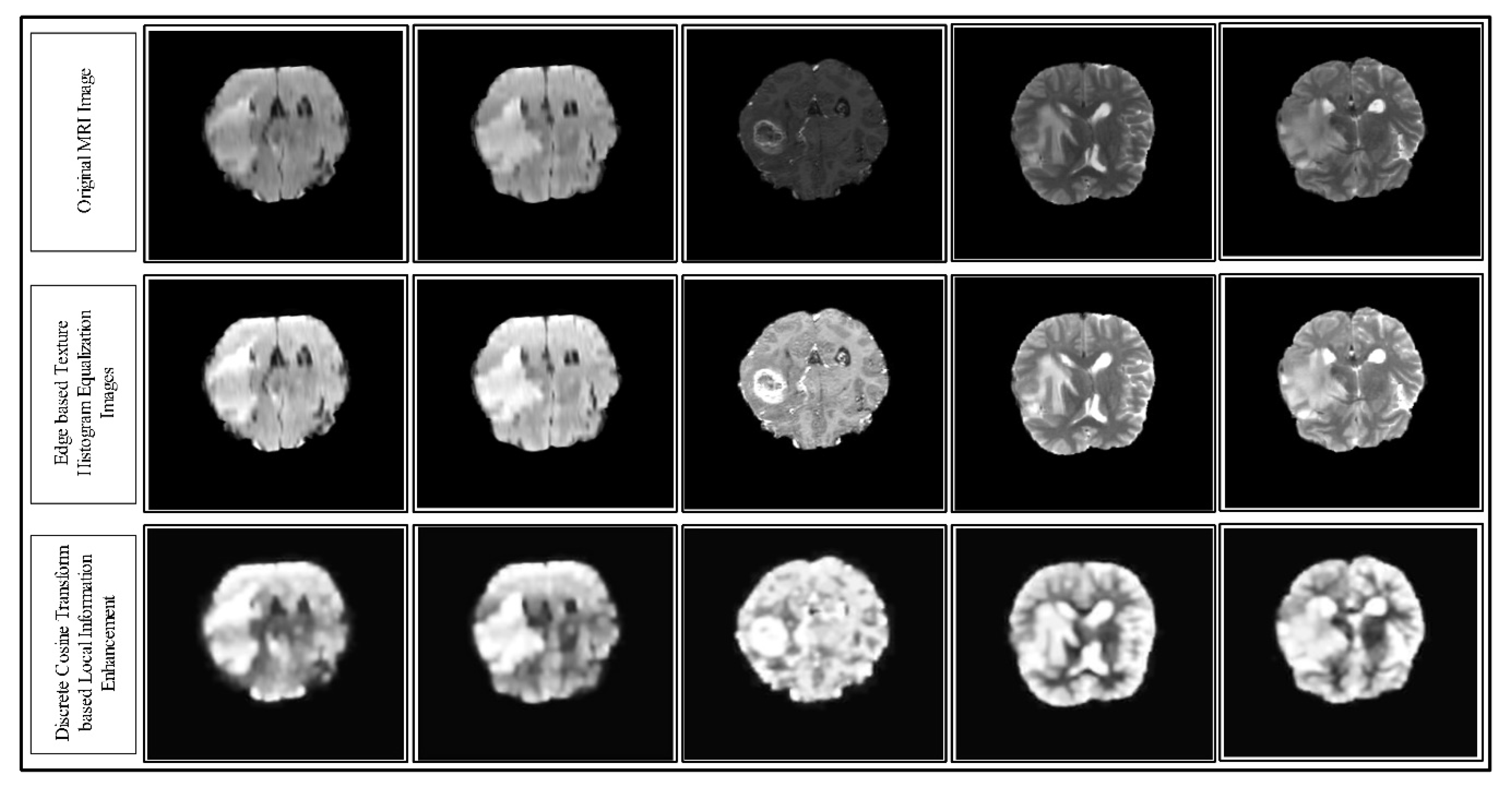
- We divided the image into two clusters based on a K-Means clustering algorithm and applied edge-based histogram equalization on each image. Further, the discrete cosine transform (DCT) was utilized for local information enhancement.
- Deep learning features were extracted from two pre-trained CNN models through transfer learning (TL). The last FC layer was used in both models for feature extraction.
- The Partial Least Square (PLS) based features of both CNN models were fused in one matrix.
- The robust features were selected using correntropy-based joint group learning. The robust features were finally classified using the ELM classifier.
- Three datasets such as BRATS 2015, BRATS 2017, and BRATS 2018 were used for the experiments and the statistical analysis to examine the scalability of the proposed classification scheme.
2. Related Work
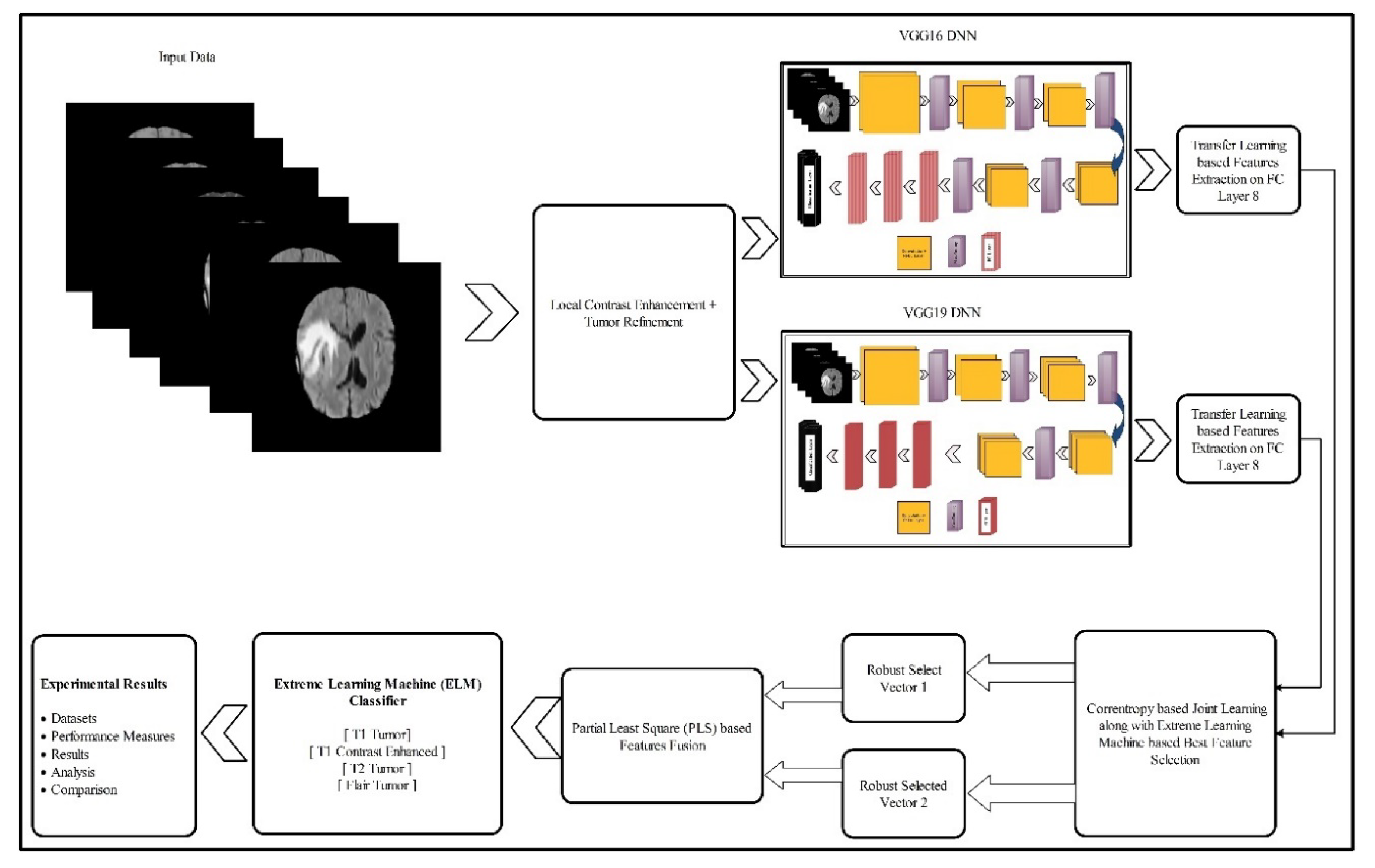
3. Proposed Methodology
3.1. Linear Contrast Enhancement
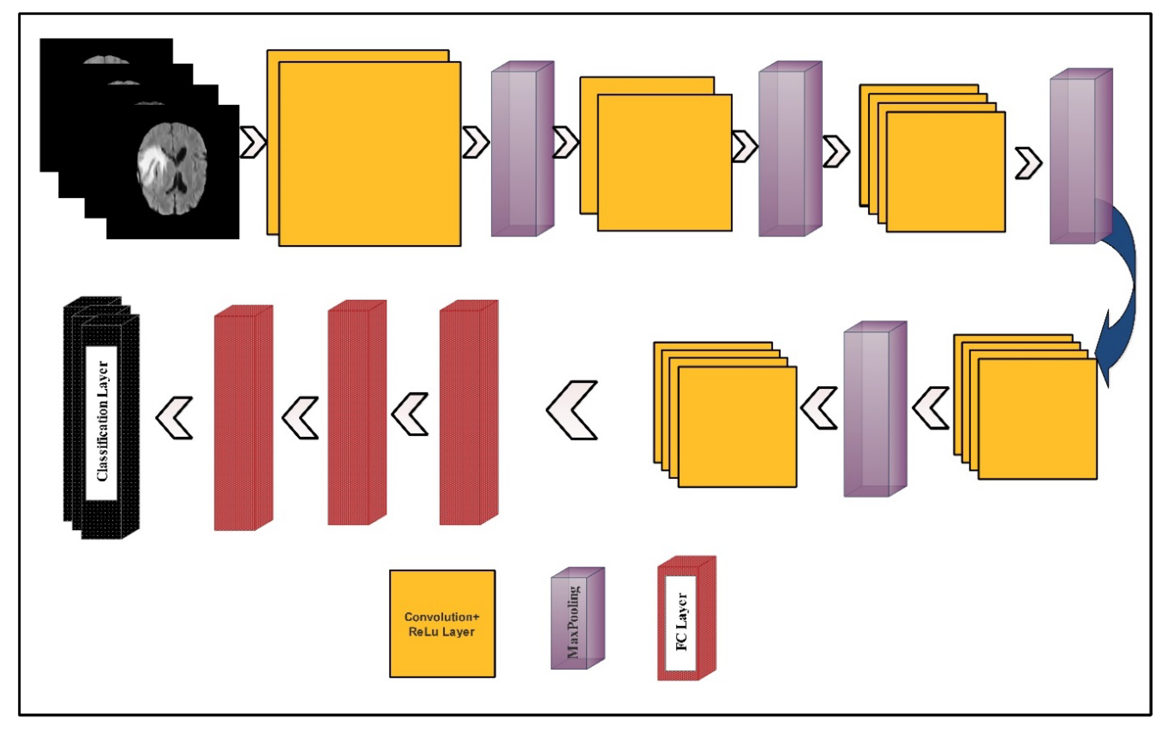
3.2. Deep Learning Features
3.3. Network Modification for Transfer Learning
3.4. Feature Selection
| Algorithm 1 Proposed feature selection method using CML-ELM. |
| Input:, |
| Output: |
| Start |
| Step 1: Parameters Initialization |
| Step 2: Forto K |
| do |
| Step 3: Update |
| Step 4: Find the minimum value ofamong, |
| ,,…) |
| :- |
| Step 5: Passed computed LR values in ELM classifier |
| Step 6: Find MSER for ELM classifier |
| Step 7: If MSER |
| Update |
| Step 8: |
| End For |
| End |
3.5. Feature Fusion and Classification
3.6. Experimental Results and Analysis
3.7. Results for the BraTS 2015 Dataset
3.8. Results for the BraTS 2017 Dataset
3.9. Results of the BraTS 2018 Dataset
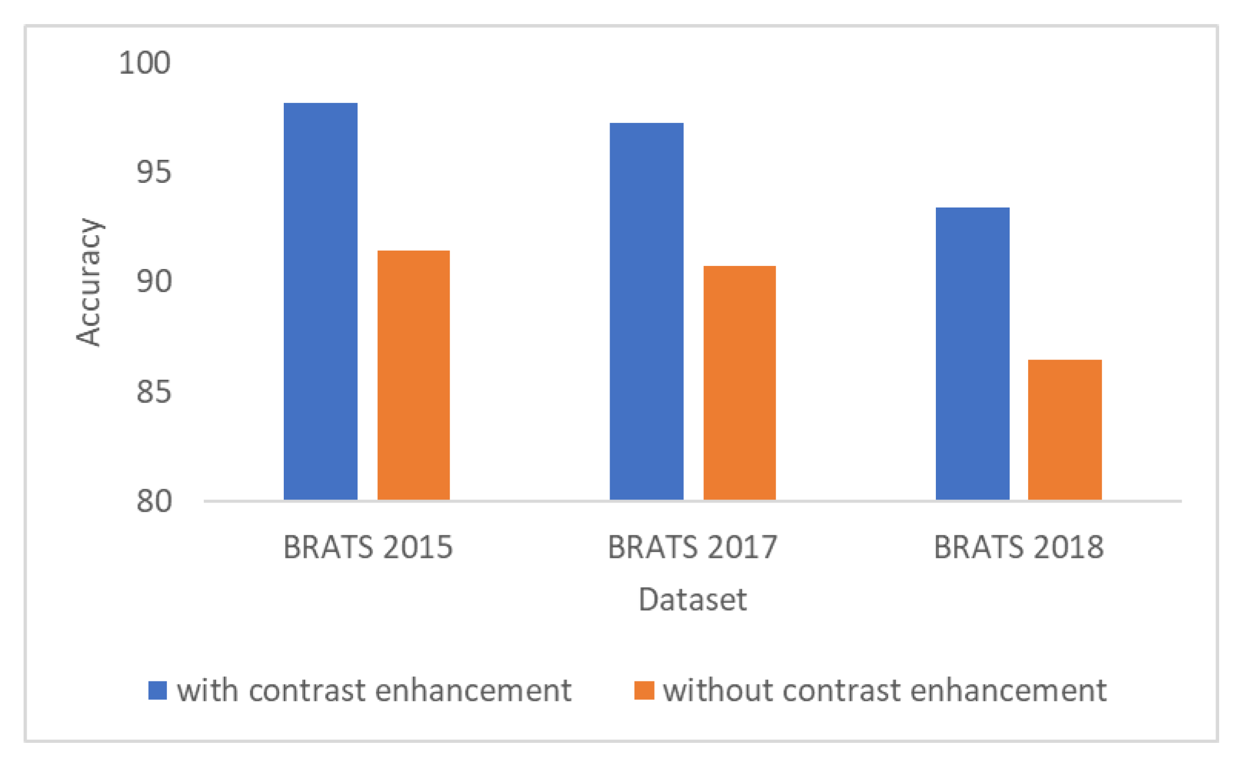
3.10. Results of the Contrast Enhancement
3.11. Statistical Analysis of Results
4. Discussion
5. Conclusions
Author Contributions
Funding
Conflicts of Interest
References
- Deepak, S.; Ameer, P. Brain tumor classification using deep CNN features via transfer learning. Comput. Biol. Med. 2019, 111, 103345. [Google Scholar] [CrossRef] [PubMed]
- Sert, E.; Özyurt, F.; Doğantekin, A. A new approach for brain tumor diagnosis system: Single image super resolution based maximum fuzzy entropy segmentation and convolutional neural network. Med. Hypotheses 2019, 133, 109413. [Google Scholar] [CrossRef] [PubMed]
- Cancer.Net, Brain Tumor Statistics. 2020. Available online: https://www.cancer.net/cancer-types/brain-tumor/statistics (accessed on 24 July 2020).
- Roy, S.; Bandyopadhyay, S.K. Detection and Quantification of Brain Tumor from MRI of Brain and It’s Symmetric Analysis. Int. J. Inf. Commun. Technol. Res. 2012, 2, 477–483. [Google Scholar]
- Pereira, S.; Pinto, A.; Alves, V.; Silva, C.A. Brain tumor segmentation using convolutional neural networks in MRI images. IEEE Trans. Med. Imaging 2016, 35, 1240–1251. [Google Scholar] [CrossRef]
- Tiwari, A.; Srivastava, S.; Pant, M. Brain tumor segmentation and classification from magnetic resonance images: Review of selected methods from 2014 to 2019. Pattern Recognit. Lett. 2020, 131, 244–260. [Google Scholar] [CrossRef]
- Hussain, U.N.; Khan, M.A.; Lali, I.U.; Javed, K.; Ashraf, I.; Tariq, J.; Ali, H.; Din, A. A Unified Design of ACO and Skewness based Brain Tumor Segmentation and Classification from MRI Scans. J. Control Eng. Appl. Inf. 2020, 22, 43–55. [Google Scholar]
- Bakas, S.; Reyes, M.; Jakab, A.; Bauer, S.; Rempfler, M.; Crimi, A.; Shinohara, R.T.; Berger, C.; Ha, S.M.; Rozycki, M. Identifying the best machine learning algorithms for brain tumor segmentation, progression assessment, and overall survival prediction in the BRATS challenge. arXiv 2018, arXiv:1811.02629. [Google Scholar]
- Chen, L.C.; Zhu, Y.; Papandreou, G.; Schroff, F.; Adam, H. Encoder-decoder with atrous separable convolution for semantic image segmentation. In Proceedings of the European Conference on Computer Vision (ECCV), Munich, Germany, 8–14 September 2018; pp. 801–818. [Google Scholar]
- Milletari, F.; Navab, N.; Ahmadi, S.A. V-net: Fully convolutional neural networks for volumetric medical image segmentation. In Proceedings of the 2016 Fourth International Conference on 3D Vision (3DV), Stanford, CA, USA, 25–28 October 2016; pp. 565–571. [Google Scholar]
- Rashid, M.; Khan, M.A.; Alhaisoni, M.; Wang, S.-H.; Naqvi, S.R.; Rehman, A.; Saba, T. A Sustainable Deep Learning Framework for Object Recognition Using Multi-Layers Deep Features Fusion and Selection. Sustainability 2020, 12, 5037. [Google Scholar] [CrossRef]
- Khan, M.A.; Khan, M.A.; Ahmed, F.; Mittal, M.; Goyal, L.M.; Hemanth, D.J.; Satapathy, S.C. Gastrointestinal diseases segmentation and classification based on duo-deep architectures. Pattern Recognit. Lett. 2020, 131, 193–204. [Google Scholar] [CrossRef]
- Majid, A.; Khan, M.A.; Yasmin, M.; Rehman, A.; Yousafzai, A.; Tariq, U. Classification of stomach infections: A paradigm of convolutional neural network along with classical features fusion and selection. Microsc. Res. Tech. 2020, 83, 562–576. [Google Scholar] [CrossRef]
- Rauf, H.T.; Shoaib, U.; Lali, M.I.; Alhaisoni, M.; Irfan, M.N.; Khan, M.A. Particle Swarm Optimization with Probability Sequence for Global Optimization. IEEE Access 2020, 8, 110535–110549. [Google Scholar] [CrossRef]
- Isensee, F.; Kickingereder, P.; Wick, W.; Bendszus, M.; Maier-Hein, K.H. Brain tumor segmentation and radiomics survival prediction: Contribution to the brats 2017 challenge. In Proceedings of the International MICCAI Brainlesion Workshop, BrainLes 2017, Quebec City, QC, Canada, 14 September 2017; pp. 287–297. [Google Scholar]
- Swati, Z.N.K.; Zhao, Q.; Kabir, M.; Ali, F.; Ali, Z.; Ahmed, S.; Lu, J. Brain tumor classification for MR images using transfer learning and fine-tuning. Comput. Med. Imaging Graph. 2019, 75, 34–46. [Google Scholar] [CrossRef] [PubMed]
- Gumaei, A.; Hassan, M.M.; Hassan, M.R.; Alelaiwi, A.; Fortino, G. A hybrid feature extraction method with regularized extreme learning machine for brain tumor classification. IEEE Access 2019, 7, 36266–36273. [Google Scholar] [CrossRef]
- Liu, J.; Liu, H.; Tang, Z.; Gui, W.; Ma, T.; Gong, S.; Gao, Q.; Xie, Y.; Niyoyita, J.P. IOUC-3DSFCNN: Segmentation of brain tumors via IOU constraint 3D symmetric full convolution network with multimodal auto-context. Sci. Rep. 2020, 10, 6256. [Google Scholar] [CrossRef] [PubMed]
- Ghassemi, N.; Shoeibi, A.; Rouhani, M. Deep neural network with generative adversarial networks pre-training for brain tumor classification based on MR images. Biomed. Signal. Process. Control 2020, 57, 101678. [Google Scholar] [CrossRef]
- Myronenko, A. 3D MRI brain tumor segmentation using autoencoder regularization. In Proceedings of the International MICCAI Brainlesion Workshop BrainLes 2018, Granada, Spain, 16 September 2018; pp. 311–320. [Google Scholar]
- Zhou, C.; Chen, S.; Ding, C.; Tao, D. Learning contextual and attentive information for brain tumor segmentation. In Proceedings of the International MICCAI Brainlesion Workshop BrainLes 2018, Granada, Spain, 16 September 2018; pp. 497–507. [Google Scholar]
- Amin, J.; Sharif, M.; Gul, N.; Yasmin, M.; Shad, S.A. Brain tumor classification based on DWT fusion of MRI sequences using convolutional neural network. Pattern Recognit. Lett. 2020, 129, 115–122. [Google Scholar] [CrossRef]
- Sajjad, M.; Khan, S.; Muhammad, K.; Wu, W.; Ullah, A.; Baik, S.W. Multi-grade brain tumor classification using deep CNN with extensive data augmentation. J. Comput. Sci. 2019, 30, 174–182. [Google Scholar] [CrossRef]
- Sharif, M.I.; Li, J.P.; Khan, M.A.; Saleem, M.A. Active deep neural network features selection for segmentation and recognition of brain tumors using MRI images. Pattern Recognit. Lett. 2020, 129, 181–189. [Google Scholar] [CrossRef]
- Seetha, J.; Raja, S.S. Brain tumor classification using convolutional neural networks. Biomed. Pharmacol. J. 2018, 11, 1457–1461. [Google Scholar] [CrossRef]
- Vijh, S.; Sharma, S.; Gaurav, P. Brain Tumor Segmentation Using OTSU Embedded Adaptive Particle Swarm Optimization Method and Convolutional Neural Network. In Data Visualization and Knowledge Engineering; Springer: Cham, Switzerland, 2020; pp. 171–194. [Google Scholar]
- Arunkumar, N.; Mohammed, M.A.; Mostafa, S.A.; Ibrahim, D.A.; Rodrigues, J.J.; de Albuquerque, V.H.C. Fully automatic model-based segmentation and classification approach for MRI brain tumor using artificial neural networks. Concurr. Comput. Pract. Exp. 2020, 32, e4962. [Google Scholar] [CrossRef]
- Sharif, M.; Amin, J.; Raza, M.; Anjum, M.A.; Afzal, H.; Shad, S.A. Brain tumor detection based on extreme learning. Neural Comput. Appl. 2020, 1–13. [Google Scholar] [CrossRef]
- Ismael, S.A.A.; Mohammed, A.; Hefny, H. An enhanced deep learning approach for brain cancer MRI images classification using residual networks. Artif. Intel. Med. 2020, 102, 101779. [Google Scholar] [CrossRef] [PubMed]
- Sharif, M.; Tanvir, U.; Munir, E.U.; Khan, M.A.; Yasmin, M. Brain tumor segmentation and classification by improved binomial thresholding and multi-features selection. J. Amb. Intel. Hum. Comp. 2018, 1–20. [Google Scholar] [CrossRef]
- Khan, M.A.; Lali, I.U.; Rehman, A.; Ishaq, M.; Sharif, M.; Saba, T.; Zahoor, S.; Akram, T. Brain tumor detection and classification: A framework of marker-based watershed algorithm and multilevel priority features selection. Microsc. Res. Tech. 2019, 82, 909–922. [Google Scholar] [CrossRef] [PubMed]
- Ke, Q.; Zhang, J.; Wei, W.; Damaševičius, R.; Woźniak, M. Adaptive independent subspace analysis of brain magnetic resonance imaging data. IEEE Access 2019, 7, 12252–12261. [Google Scholar] [CrossRef]
- Rehman, A.; Naz, S.; Razzak, M.I.; Akram, F.; Imran, M. A deep learning-based framework for automatic brain tumors classification using transfer learning. Circ. Syst. Signal. Pr. 2020, 39, 757–775. [Google Scholar] [CrossRef]
- Ghosal, P.; Nandanwar, L.; Kanchan, S.; Bhadra, A.; Chakraborty, J.; Nandi, D. Brain Tumor Classification Using ResNet-101 Based Squeeze and Excitation Deep Neural Network. In Proceedings of the Second International Conference on Advanced Computational and Communication Paradigms (ICACCP), Gangtok, India, 25–28 February 2019; pp. 1–6. [Google Scholar]
- Toğaçar, M.; Cömert, Z.; Ergen, B. Classification of brain MRI using hyper column technique with convolutional neural network and feature selection method. Expert Syst. Appl. 2020, 149, 113274. [Google Scholar] [CrossRef]
- Muhammad, K.; Khan, S.; Del Ser, J.; de Albuquerque, V.H.C. Deep Learning for Multigrade Brain Tumor Classification in Smart Healthcare Systems: A Prospective Survey. IEEE Trans. Neural Netw. Learn. Syst. 2020. [Google Scholar] [CrossRef]
- Rehman, A.; Khan, M.A.; Mehmood, Z.; Saba, T.; Sardaraz, M.; Rashid, M. Microscopic melanoma detection and classification: A framework of pixel-based fusion and multilevel features reduction. Microsc. Res. Tech. 2020, 83, 410–423. [Google Scholar] [CrossRef]
- Khan, M.A.; Sharif, M.; Akram, T.; Bukhari, S.A.C.; Nayak, R.S. Developed Newton-Raphson based deep features selection framework for skin lesion recognition. Pattern Recognit. Lett. 2020, 129, 293–303. [Google Scholar] [CrossRef]
- Gabryel, M.; Damaševičius, R. The image classification with different types of image features. In Proceedings of the International Conference on Artificial Intelligence and Soft Computing, ICAISC 2017, Zakopane, Poland, 11–15 June 2017; pp. 497–506. [Google Scholar] [CrossRef]
- Khan, M.A.; Rubab, S.; Kashif, A.; Sharif, M.I.; Muhammad, N.; Shah, J.H.; Zhang, Y.-D.; Satapathy, S.C. Lungs cancer classification from CT images: An integrated design of contrast based classical features fusion and selection. Pattern Recognit. Lett. 2020, 129, 77–85. [Google Scholar] [CrossRef]
- Chouhan, V.; Singh, S.K.; Khamparia, A.; Gupta, D.; Tiwari, P.; Moreira, C.; Damaševičius, R.; de Albuquerque, V.H.C. A novel transfer learning based approach for pneumonia detection in chest X-ray images. Appl. Sci. 2020, 10, 559. [Google Scholar] [CrossRef] [Green Version]
- Ke, Q.; Zhang, J.; Wei, W.; Połap, D.; Woźniak, M.; Kośmider, L.; Damaševičius, R. A neuro-heuristic approach for recognition of lung diseases from X-ray images. Expert Syst. Appl. 2019, 126, 218–232. [Google Scholar] [CrossRef]
- Weiss, K.; Khoshgoftaar, T.M.; Wang, D. A survey of transfer learning. J. Big Data 2016, 3, 9. [Google Scholar] [CrossRef] [Green Version]
- Huang, G.-B.; Zhu, Q.-Y.; Siew, C.-K. Extreme learning machine: A new learning scheme of feedforward neural networks. In Proceedings of the 2004 IEEE International Joint Conference on Neural Networks, Budapest, Hungary, 25–29 July 2004; pp. 985–990. [Google Scholar]


| Classifier | Feature Selection Technique | Validation Measures | ||
|---|---|---|---|---|
| Accuracy (%) | FNR (%) | Testing Time (s) | ||
| Naïve Bayes | Pro-FC7 | 93.29 | 6.71 | 117.68 |
| Proposed | 94.19 | 5.81 | 104.02 | |
| MSVM | Pro-FC7 | 92.59 | 7.41 | 136.31 |
| Proposed | 94.66 | 5.34 | 101.66 | |
| Softmax | Pro-FC7 | 91.48 | 8.52 | 96.69 |
| Proposed | 93.98 | 6.02 | 81.02 | |
| Ensemble Tree | Pro-FC7 | 92.43 | 7.57 | 137.60 |
| Proposed | 95.67 | 4.33 | 104.59 | |
| ELM | Pro-FC7 | 96.02 | 3.98 | 99.42 |
| Proposed | 98.16 | 1.74 | 87.41 | |
| Class | T1 | T1CE | T2 | Flair |
|---|---|---|---|---|
| T1 | 98.42% | <1% | 0% | <1% |
| T1CE | 1% | 96.00% | 2% | 1% |
| T2 | 0% | 0% | 99.46% | <1% |
| Flair | <1% | <1% | <1% | 98.80% |
| Class | T1 | T1CE | T2 | Flair |
|---|---|---|---|---|
| T1 | 97.16% | <1% | 2% | 0% |
| T1CE | <1% | 95.24% | 3% | 1% |
| T2 | <1% | 2% | 97.60% | 0% |
| Flair | 0% | 2% | 3% | 94.00% |
| Classifier | Feature Selection Technique | Validation Measure | ||
|---|---|---|---|---|
| Accuracy (%) | FNR (%) | Testing Time (s) | ||
| Naïve Bayes | Pro-FC7 | 91.59 | 8.41 | 197.46 |
| Proposed | 93.66 | 6.34 | 104.59 | |
| MSVM | Pro-FC7 | 90.09 | 9.91 | 211.62 |
| Proposed | 94.58 | 5.42 | 171.42 | |
| Softmax | Pro-FC7 | 91.67 | 8.33 | 111.44 |
| Proposed | 93.98 | 6.02 | 91.25 | |
| Ensemble Tree | Pro-FC7 | 93.69 | 6.31 | 147.38 |
| Proposed | 95.42 | 4.58 | 101.29 | |
| ELM | Pro-FC7 | 95.82 | 4.18 | 107.59 |
| Proposed | 97.26 | 2.74 | 89.64 | |
| Class | T1 | T1CE | T2 | Flair |
|---|---|---|---|---|
| T1 | 96.24% | 2% | 1% | <1% |
| T1CE | <1% | 98.66% | 0% | 1% |
| T2 | 2% | 0% | 97.20 | <1% |
| Flair | 1% | 0% | 2% | 97.00% |
| Class | T1 | T1 CE | T2 | Flair |
|---|---|---|---|---|
| T1 | 94.20% | 4% | 1% | <1% |
| T1 CE | 4% | 94.84% | 3% | 2% |
| T2 | 0% | 3% | 96.68% | <1% |
| Flair | <1% | 1% | 2% | 96.02% |
| Classifier | Feature Selection Technique | Validation Measure | ||
|---|---|---|---|---|
| Accuracy | FNR | Testing Time (s) | ||
| Naïve Bayes | Pro-FC7 | 87.63 | 12.37 | 204.31 |
| Proposed | 89.49 | 10.51 | 117.62 | |
| MSVM | Pro-FC7 | 88.19 | 11.81 | 207.56 |
| Proposed | 91.34 | 8.66 | 167.49 | |
| Softmax | Pro-FC7 | 90.26 | 9.74 | 131.31 |
| Proposed | 92.42 | 7.58 | 91.63 | |
| Ensemble Tree | Pro-FC7 | 89.16 | 10.84 | 151.34 |
| Proposed | 91.79 | 8.21 | 106.12 | |
| ELM | Pro-FC7 | 91.69 | 8.31 | 97.04 |
| Proposed | 93.40 | 6.60 | 63.83 | |
| Class | T1 | T1CE | T2 | Flair |
|---|---|---|---|---|
| T1 | 89.40% | 7% | <1% | 3% |
| T1CE | 3% | 94.60% | <1% | 2% |
| T2 | 2% | 4% | 93.20% | <1% |
| Flair | 1% | 0% | 3% | 96.00% |
| Class | T1 | T1CE | T2 | Flair |
|---|---|---|---|---|
| T1 | 88.18% | 6% | 3% | <3% |
| T1CE | <1% | 92.16% | 6% | 1% |
| T2 | 1% | 7% | 91.62% | <1% |
| Flair | 2% | <1% | 5% | 92.14% |
| Method | Min (%) | Avg (%) | Max (%) | SEM | ||
|---|---|---|---|---|---|---|
| Naïve Bayes | 92.47 | 93.33 | 94.9 | 0.493 | 0.7021 | 0.4054 |
| MSVM | 92.19 | 93.42 | 96.66 | 1.016 | 1.0083 | 0.5821 |
| Softmax | 91.63 | 92.8 | 93.98 | 0.920 | 0.9593 | 0.5539 |
| ET | 92.98 | 94.32 | 95.67 | 1.206 | 1.0981 | 0.6340 |
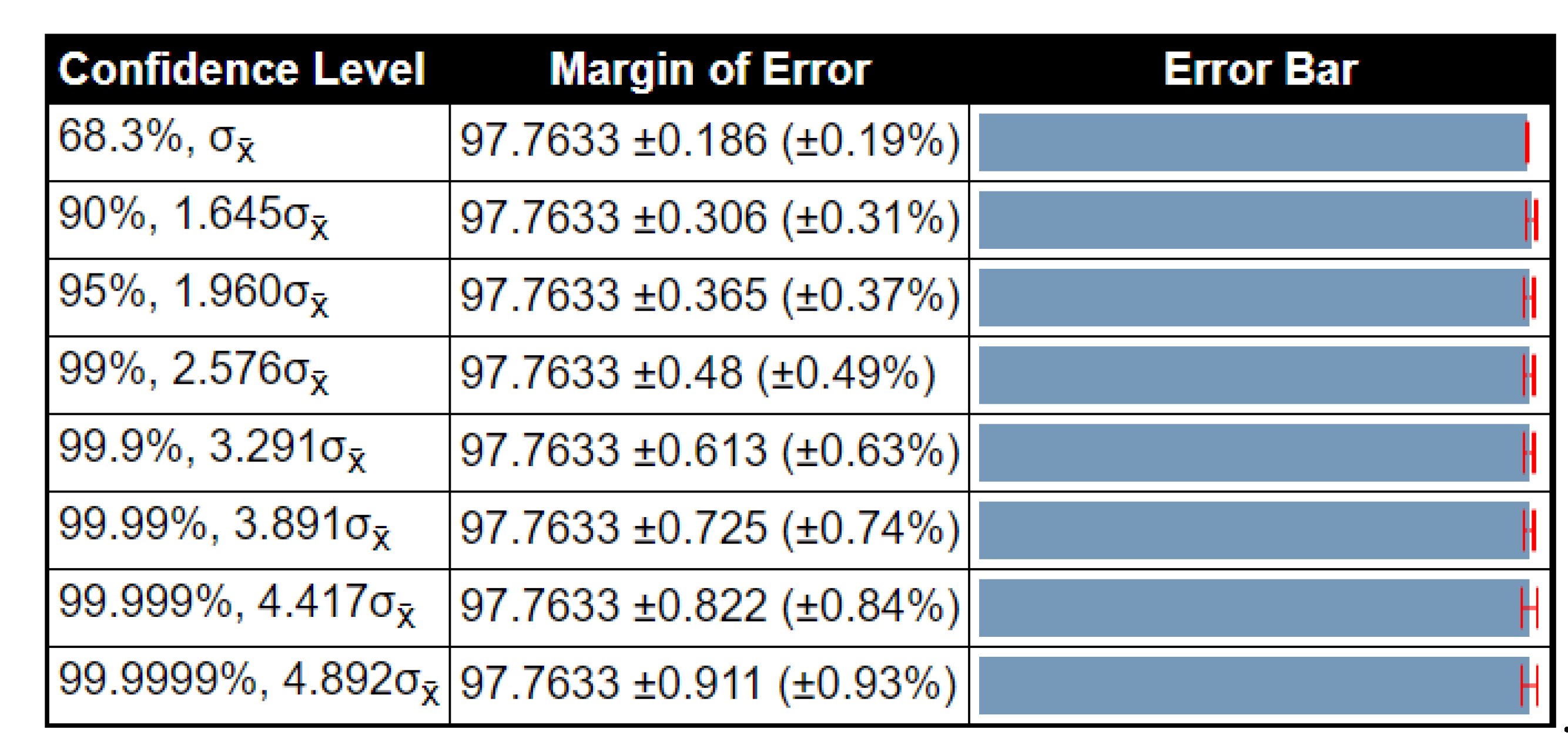
| ELM | 97.37 | 97.76 | 98.16 | 0.104 | 0.3225 | 0.1862 |
| Method | Min (%) | Avg (%) | Max (%) | SEM | ||
|---|---|---|---|---|---|---|
| Naïve Bayes | 91.04 | 92.35 | 93.66 | 1.144 | 1.0696 | 0.6175 |
| MSVM | 92.67 | 93.62 | 94.58 | 0.608 | 0.7797 | 0.451 |
| Softmax | 90.29 | 92.13 | 93.98 | 2.2693 | 1.5064 | 0.8697 |
| ET | 93.16 | 94.29 | 95.42 | 0.8512 | 0.9226 | 0.5326 |
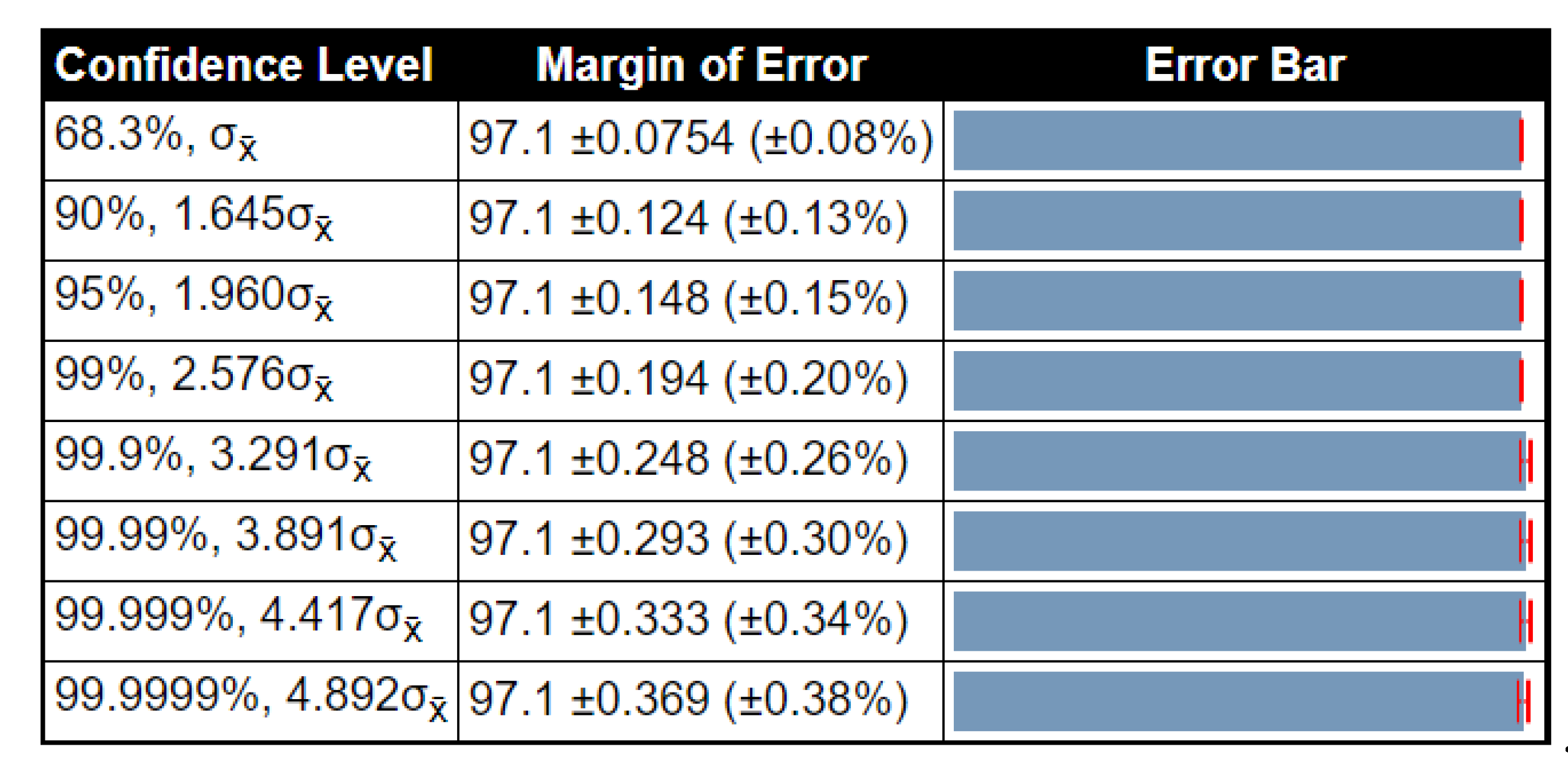
| ELM | 96.94 | 97.1 | 97.26 | 0.017 | 0.1306 | 0.0754 |
| Method | Min (%) | Avg (%) | Max (%) | SEM | ||
|---|---|---|---|---|---|---|
| Naïve Bayes | 87.42 | 88.45 | 89.49 | 0.7141 | 0.8450 | 0.4879 |
| MSVM | 86.69 | 90.01 | 91.34 | 1.1704 | 1.0818 | 0.6246 |
| Softmax | 91.04 | 91.73 | 92.42 | 0.3174 | 0.5633 | 0.3252 |
| ET | 88.64 | 90.21 | 91.79 | 1.6537 | 1.2859 | 0.7424 |
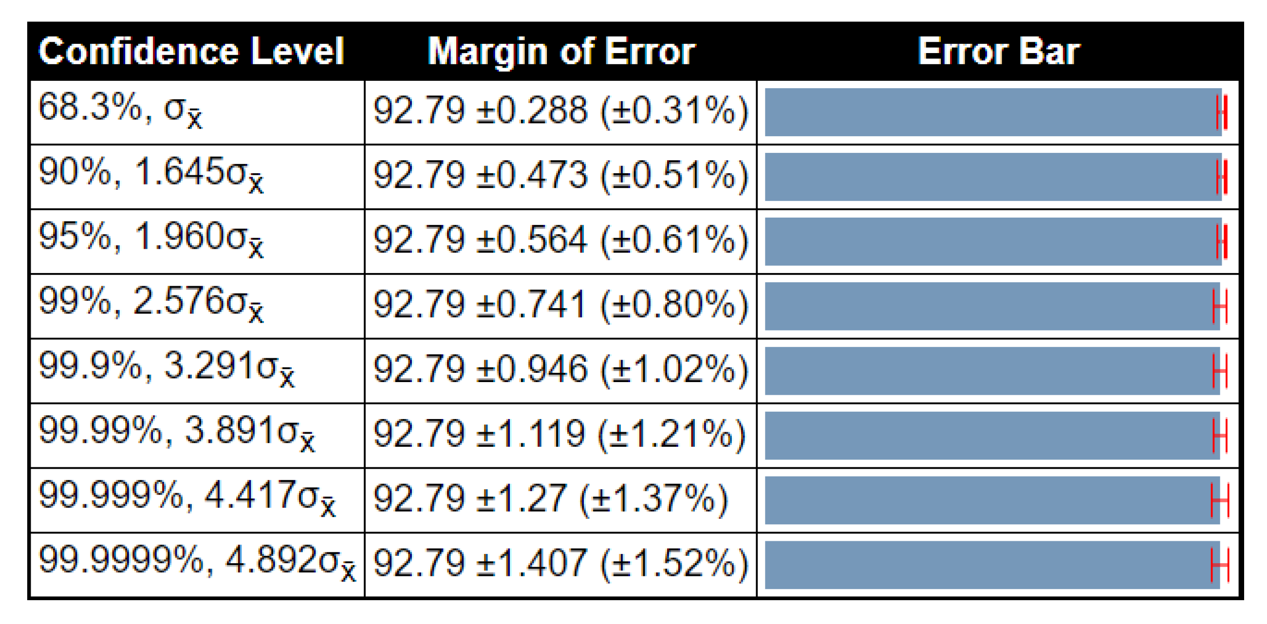
| ELM | 92.18 | 92.79 | 93.40 | 0.2480 | 0.4980 | 0.2875 |
| Dataset | Pro-FC7 | Proposed | MCC |
|---|---|---|---|
| BRATS2015 | √ | 0.8690 | |
| √ | 0.8804 | ||
| BRATS2017 | √ | 0.8523 | |
| √ | 0.8764 | ||
| BRATS2018 | √ | 0.8036 | |
| √ | 0.8244 |
© 2020 by the authors. Licensee MDPI, Basel, Switzerland. This article is an open access article distributed under the terms and conditions of the Creative Commons Attribution (CC BY) license (http://creativecommons.org/licenses/by/4.0/).
Share and Cite
Khan, M.A.; Ashraf, I.; Alhaisoni, M.; Damaševičius, R.; Scherer, R.; Rehman, A.; Bukhari, S.A.C. Multimodal Brain Tumor Classification Using Deep Learning and Robust Feature Selection: A Machine Learning Application for Radiologists. Diagnostics 2020, 10, 565. https://doi.org/10.3390/diagnostics10080565
Khan MA, Ashraf I, Alhaisoni M, Damaševičius R, Scherer R, Rehman A, Bukhari SAC. Multimodal Brain Tumor Classification Using Deep Learning and Robust Feature Selection: A Machine Learning Application for Radiologists. Diagnostics. 2020; 10(8):565. https://doi.org/10.3390/diagnostics10080565
Chicago/Turabian StyleKhan, Muhammad Attique, Imran Ashraf, Majed Alhaisoni, Robertas Damaševičius, Rafal Scherer, Amjad Rehman, and Syed Ahmad Chan Bukhari. 2020. "Multimodal Brain Tumor Classification Using Deep Learning and Robust Feature Selection: A Machine Learning Application for Radiologists" Diagnostics 10, no. 8: 565. https://doi.org/10.3390/diagnostics10080565