Dynamic Handling Characterization and Set-Up Optimization for a Formula SAE Race Car via Multi-Body Simulation

Abstract

There is a growing interest towards multi-body modelling and simulation that play a critical role in the development and testing of new mechanical systems, in general, and formula cars specifically to avoid expensive and time-consuming experimental track testing. Recent advances in computer-aided engineering packages, allows one not only to evaluate the basic properties that define the dynamic behavior of a newly-designed formula car, but as well as to investigate the impact on the performance of the many adjustable parameters that collectively are referred to as the car set-up. Therefore, by providing a rapid feedback of a given set-up expectation, optimal configurations can be obtained ensuring the highest level of performance. In this paper, a Formula SAE vehicle is expressly targeted. First, a full multi-body model of the prototype is described detailing the properties of each subassembly, e.g., suspensions and antiroll bars, steering system, and powertrain. Then, the basic handling characteristics are obtained via simulated track testing. Based on vehicle dynamics principles, the fine tuning of the vehicle setup is thoroughly discussed to gain the best performance in each of the contest events of the Formula SAE competition. For example, in the skidpad event where cars are required to drive along an eight-shaped track, an almost 2 km/h gain in the maximum travel velocity can be achieved by adjusting the camber angles of all tires.

1. Introduction

The Society of Automotive Engineers (SAE) sponsors the student competition Formula SAE (FSAE) where worldwide students are involved in a contest to design, build and race using a scaled-down formula car [1]. The FSAE contest comprises static and dynamic events. The former are the cost assessment, business plan, and engineering design. The dynamic events include a skid-pad of 15.25 m diameter, an acceleration test of 75 m, 1500 m autocross, endurance race of 22,000 m and fuel consumption [2].

The handling properties of a formula car depend on the interplay of many parameters [3]. Some of them are set during the design stage and cannot be changed after the car has been assembled. The vehicle mass, location of the center of mass, the attachment points of the front and rear suspension system on the chassis are examples of these “fixed” parameters. Nevertheless, the vehicle response and overall performance can be fine-tuned by operating on a set of adjustable parameters including tire inflation pressure, suspension and roll stiffness, braking ratio and tire camber angle. The parameters that can be adjusted to control the handling properties are collectively referred to as the “set-up” of the car. It should be noted that for a race car, it is very difficult or impossible to find a single optimal set-up that ensures the highest level of performance in any race track and contest event. If one set-up performs well over a certain track, it does not mean that the same set-up will provide the best performance in another track or different event.

Typically, engineers change vehicle configurations to correct low performing response. This is done manually via successive adjustments that can be tedious and often made ad-hoc, which adversely affects the quality of the overall engineering process. Car set-up is performed via a laborious heuristic approach through which engineers adjust some car parameters and drivers evaluate the car performance on track, usually performed during testing session before the event. This approach is tightly connected with the knowledge developed by the engineers through experience. It does not guarantee the delivery of the full potential of a formula car. Often, car set-up provides sub-optimal performance levels.

Pursuing the objective to avoid, as much as possible, any manual adjustment while improving at the same time the overall quality of the intended regulations, this paper presents a comprehensive approach to modelling, simulation, and optimization of formula cars that draws on vehicle dynamic principles. The virtual prototyping model of FSAE race car is built by a multi-body dynamics simulation software. The ability to compute, test, assess, and debug suitable configurations would reduce the time and cost of vehicle development. Performance prediction and optimization based on virtual prototyping technology would contribute to reach more easily the optimal set-up for any given event or race.

Related research efforts have been devoted to the introduction and development of modern design methodologies. The typical engineering design of a formula car comprises three main stages: definition of the technical requirements, building of the vehicle to fulfil these specifications and performance of test runs on track for fine-tuning of vehicle parameters towards performance maximization.

In the last few years, virtual prototyping has attracted much attention as a key technology that allows the conceptualization, design, and optimization of vehicles to be improved and streamlined by simulation [4]. These testbeds provide the ability to interact with the prototype to get an in-depth understanding of possible flaws as early as possible during the design process. Typical application fields are space robotics [5,6,7,8], marine [9] and ground vehicles [10], whether manned [11] or unmanned [12]. Virtual prototypes offer a sophisticated physically based simulation of both the vehicle and its operating field, along with real-time, immersive rendering and 3D interaction methods for direct feedback and manipulation of the vehicle. Beyond the design stage, the same virtual testbeds can be re-used as well for training and supervision purposes. Finally, virtual prototyping can be a cost-efficient solution in applications such as planetary exploration missions or autonomous driving where setting up real mockups for testing would be too expensive [13].

In this study, the dynamics simulation software MSC Adams is used to virtual prototyping a FSAE race car. MSC Adams was used in previous research to evaluate the stability to crosswind in FSAE racing cars [14] and to analyze the performance of single vehicle subsystems including the suspension system [15,16,17]. Here, the problem of full-vehicle handling characterization and set-up optimization is tackled to gain the highest level of performance in the contest events of the FSAE competition. Even when considering advanced virtual environments, it is still challenging to identify the underlying mechanisms that govern the system dynamic response. In this respect, it is important to put forward the principles of vehicle dynamics. Throughout the paper, basic knowledge of vehicle and suspension design is assumed.

Section 2 recalls principles of multi-body dynamic analysis, whereas Section 3 presents the vehicle full assembly providing details about the different car subcomponent. The characterization of the handling properties is described in Section 4, where the set of adjustable parameters that defines the set-up of the car is defined as well. Section 5 describes the set-up optimization for the main events of the formula SAE contest. Conclusions and lessons learned are drawn in Section 6.

2. Basis of Multi-Body Dynamics

For any given multi-body systems (MBS) being considered, the position problem consists of solving the constraint equations, which form the following set of equations:

$$\phi \left(\mathit{q},t\right)=0$$

(1)

where q is the vector of the system generalized coordinates. It is assumed that the number of equations is equal to the number of unknown variables. By taking first derivative of Equation (1), the velocity kinematic constraint equations are obtained as

$${\mathit{\phi }}_{\mathit{q}}\dot{\mathit{q}}=0$$

(2)

${\mathit{\phi }}_{\mathit{q}}$being the Jacobian matrix of Equation (1) with respect to q, and $\dot{q}$ the vector of generalized velocities. By differentiating Equation (2), one obtains the acceleration kinematic equations:

$${\mathit{\phi }}_{\mathit{q}}\ddot{\mathit{q}}=-{\dot{\mathit{\phi }}}_{\mathit{q}}\dot{\mathit{q}}$$

(3)

where $\ddot{\mathit{q}}$ is the vector of generalized accelerations. Equations (1) through (3) can be seen as constraints that the generalized coordinates and corresponding derivates must fulfill for a consistent time evolution of the system under investigation.

By applying the classical Newton’s law and by taking into account constraints, the dynamic problem can be addressed through the following set of differential equations

$$\mathit{M}\ddot{\mathit{q}}+{\mathit{\phi }}_{\mathit{q}}{}^{\mathit{T}}\mathit{\lambda }=\mathit{Q}$$

(4)

M being the mass matrix, Q the vector containing the external forces and $\mathit{\lambda }$ the vector of Lagrangian multipliers. By adding the m Equations (3), Equation (4), which is a system of n equations (n: number of dofs) in n + m variables, can be solved as

$$\left[\begin{array}{cc}\mathit{M}& {\mathit{\phi }}_{\mathit{q}}{}^{\mathit{T}}\\ {\mathit{\phi }}_{\mathit{q}}& \mathbf{0}\end{array}\right]\left[\begin{array}{c}\ddot{\mathit{q}}\\ \mathit{\lambda }\end{array}\right]=\left[\begin{array}{c}\mathit{Q}\\ \mathit{\tau }\end{array}\right]$$

(5)

The system of Equation (5) can be used for simultaneous solution of the accelerations and Lagrange multipliers [18].

3. Full-Vehicle Modeling via Multi-Body Approach

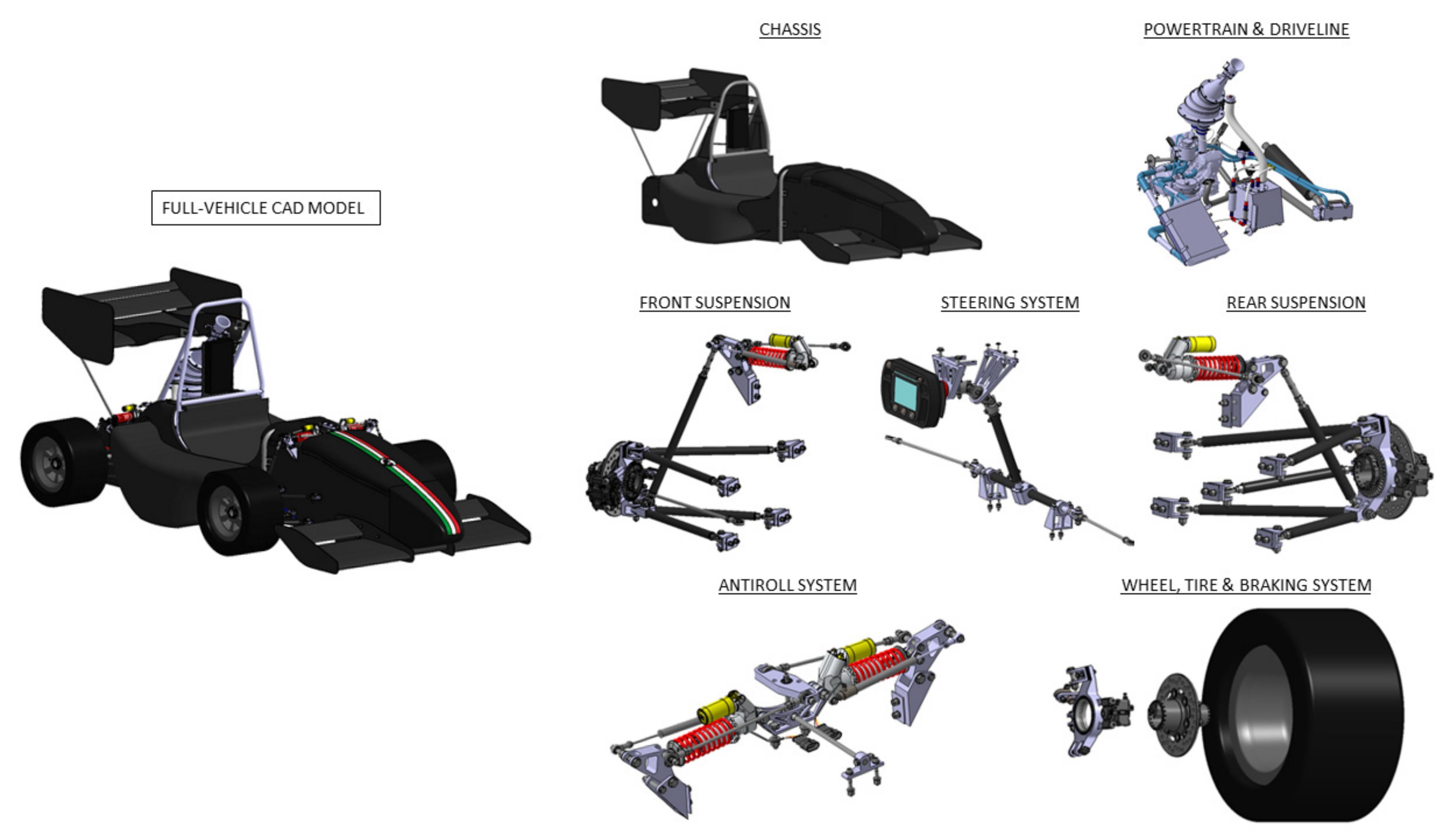
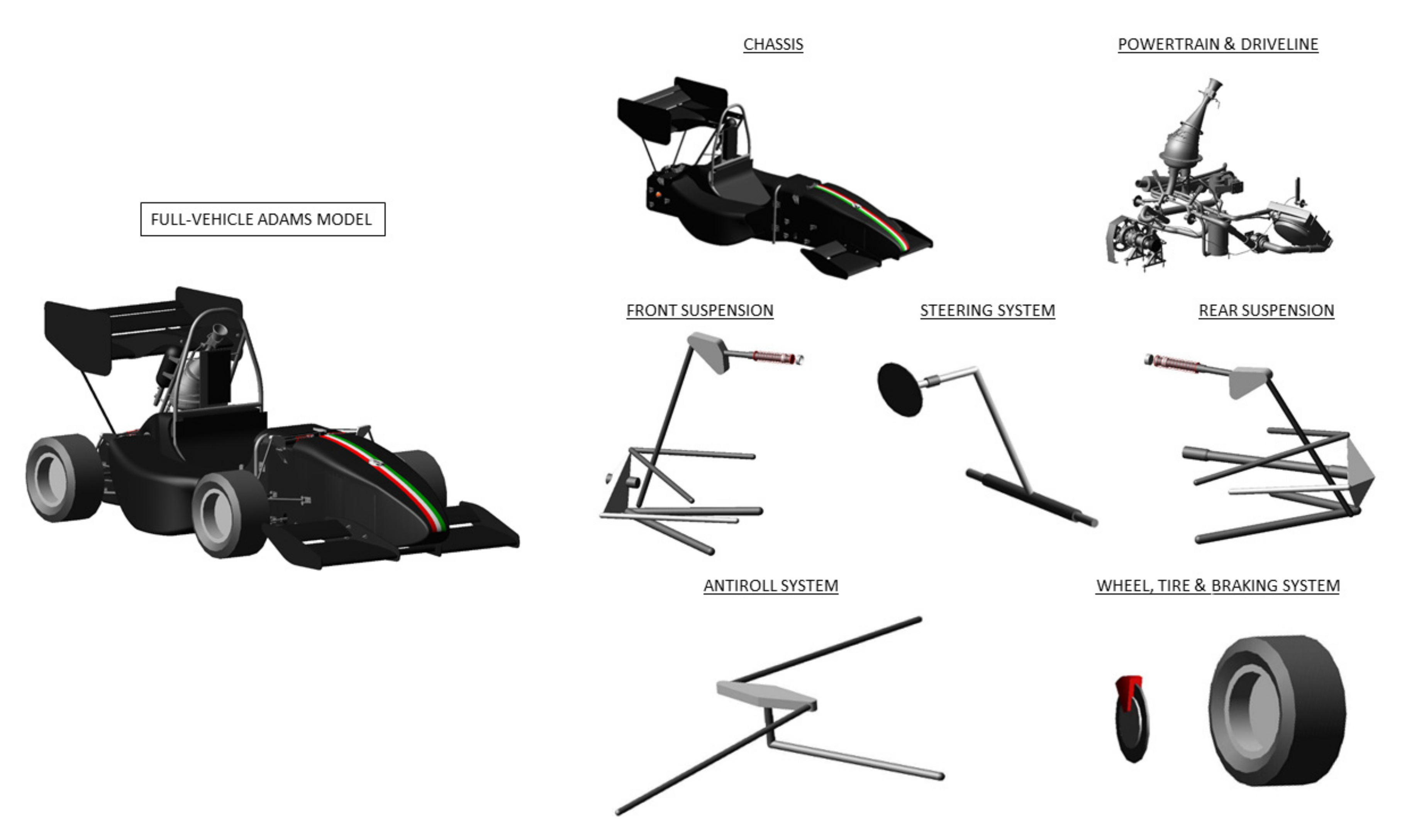
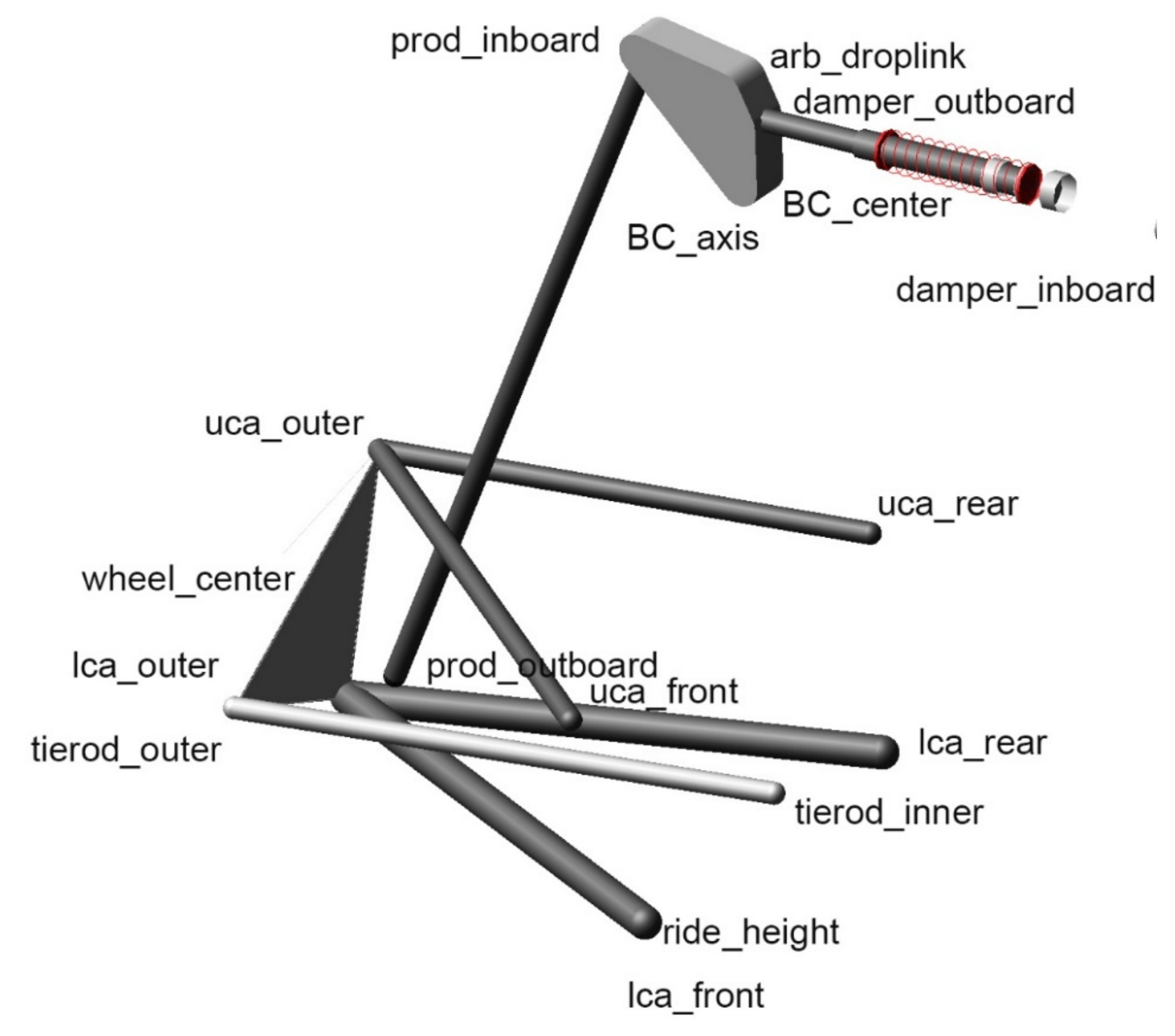
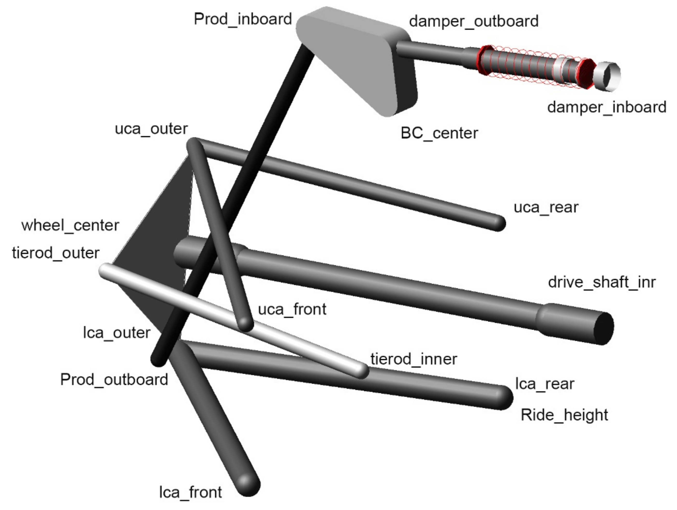
In order to create and simulate the dynamics of a full vehicle system, many sub-systems need to be modelled and assembled. The chassis, engine, driveline, and body areas of the vehicle are examples of components that can be modelled and simulated through the use of modern multi-body systems (MBS) software (2017.2, MSC Adams, Newport Beach, California) [19]. Figure 1 and Figure 2 explain well the concept. MBS models for the main sub-systems are linked together to build a detailed “literal” representation of the full vehicle. Suspension systems, anti-roll bars, steering mechanism, brake system and drive inputs to the wheels are all modelled to a level appropriate for a high-fidelity simulation of the vehicle dynamics. It will be assumed that the chassis and suspension can be treated as rigid bodies, resulting in some errors because the compliance characteristic of chassis and suspension is neglected.

The vehicle features monocoque type chassis ensuring at the same time lightness and high torsional stiffness. The aerodynamic package comprises a front wing, lateral badge board and a rear wing. Both front and rear suspensions follow a double-wishbone solution with carbon fiber links and push-rod system, adjustable anti-roll bars, and a steering system with aluminum rack and carbon steering column and wheel.

The tire assembly is composed by magnesium rims of 10 inch, slick and radial-ply tires, Al7075 hubs and uprights, and disk brakes with aluminum pads with high efficiency and adjustable brake balance. The powertrain comprises a twin-cylinder 550 cc engine, nylon 3D printed intake and titanium alloy exhaust, equipped with specific differential for formula SAE with electro pneumatic shift.

Finally, the overall vehicle dimensions are 1.55 m wheelbase with 1.15 m front track and 1.10 m rear track. The combined ready-to-race vehicle/driver total weight is 275 kg, with 50/50 front/rear distribution. All subcomponents have been accurately modelled in MSC Adams [20], as shown Figure 2 to reflect with high fidelity the geometric and inertial properties. Hoosier 43105 R25B tires (Hoosier Racing Tire, Lakeville, IN, USA) have been simulated adopting a PAC2002 model [21], whose parameters were obtained by fitting the measurement data for the whole range of tire behavior available through the FSAE Tire Test consortium [22]. For confidentiality reasons, details are not reported here. However, “.tir” files used in the simulations are available upon requests. Further details of the multi-body Formula Student assembly can be found in Appendix A.

4. Dynamic Handling Characterization and Baseline Vehicle Set-Up

Vehicle handling properties can be typically evaluated by referring to the understeer gradient $K_{US}$ that defines the under/oversteer tendency [19]. With reference to an equivalent single-track model, the fundamental handling relation at steady-state can be expressed by the following:

$${\delta }_p=\frac{l}{R}+K_{US}\frac{a_y}{g}$$

(6)

where

• ${\delta }_p$ is the front tire steer angle;
• $l$ is the vehicle wheelbase;
• $R$ is the cornering radius;
• $a_y$ is the lateral acceleration;
• $g$ is the gravity acceleration.

In practice, the understeer gradient can be determined finding the relationship between the tire steer angle and the lateral acceleration via track testing, performing for example a set of step-steer maneuvers. Here, the same “experimental” procedure is performed via MBS simulation.

Since a direct measurement of the tire steer angle tice, ${\delta }_p$ is difficult in practice, it is indirectly estimated via the measurement of the steering wheel angle that can be obtained using, for example, a “virtual” rotary potentiometer. The transmission ratio between the tire steer angle and the steering wheel angle needs to be introduced ${\tau }_s=\frac{{\delta }_p}{{\delta }_v}$ and measured. To this aim, a so-defined geometrically-correct or Ackermann steering maneuver is simulated where the vehicle follows a skid-pad of known radius (R = 50 m) at low speed (about 4 km/h). At this speed, the tire slip angles can be neglected and Equation (6) reduces to ${\delta }_p=\frac{l}{R}$. The results obtained in the simulation are collected in

Table 1. Results obtained in the Ackermann steering maneuver.

Parameter	Value
$l$	$1.55 \mathrm{m}$
${\delta }_v$	$0.170 \mathrm{rad}$
${\delta }_p$	$0.031 \mathrm{rad}$
${\tau }_s$	$0.182$

:

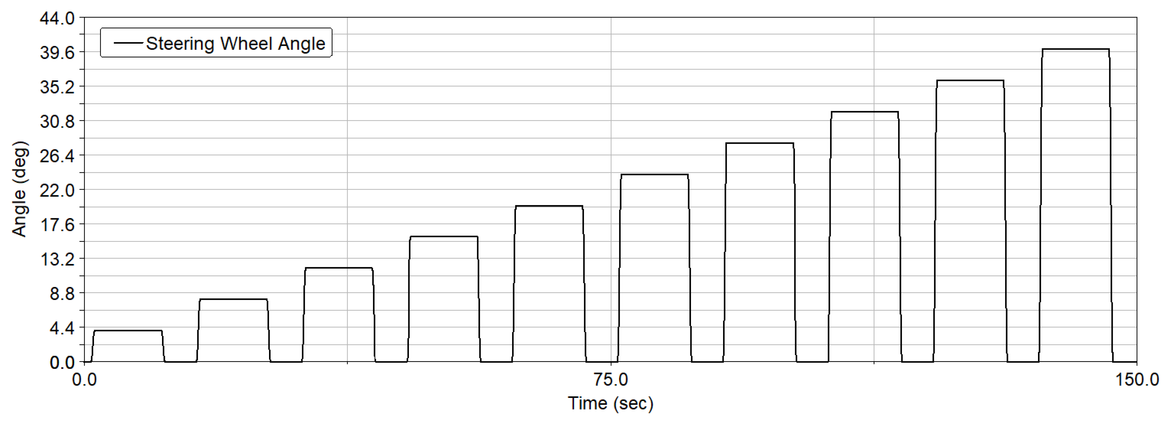
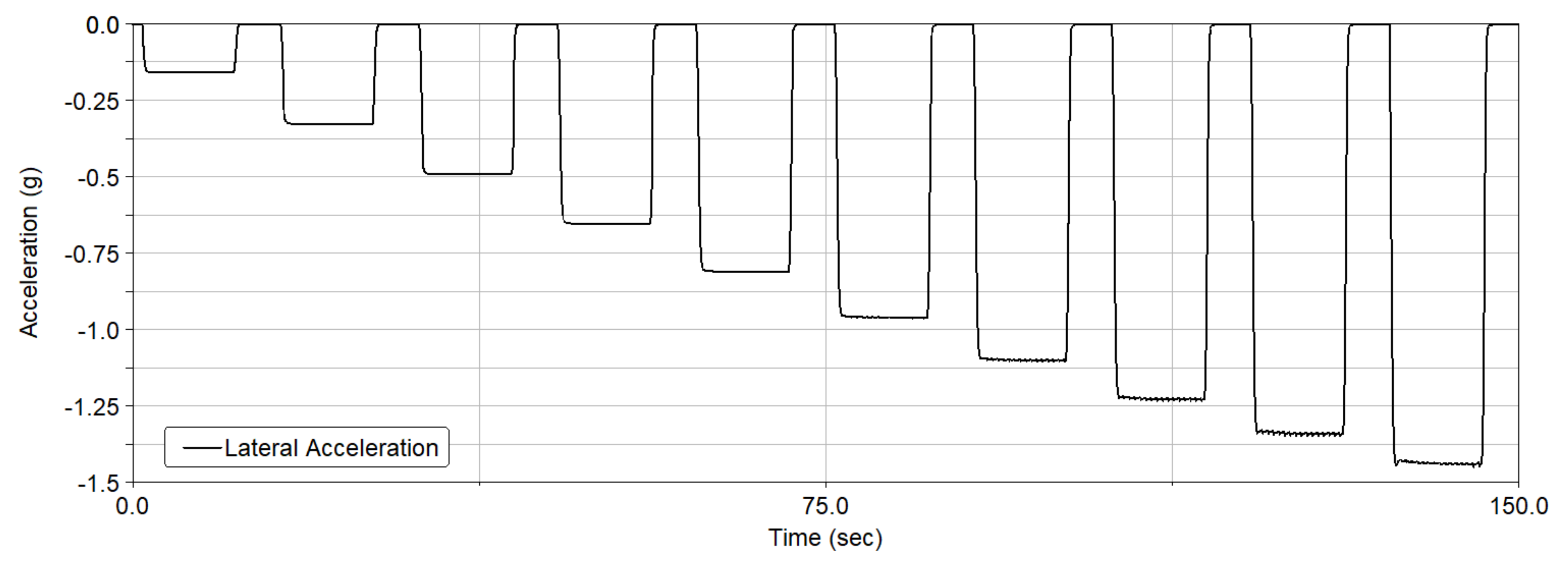
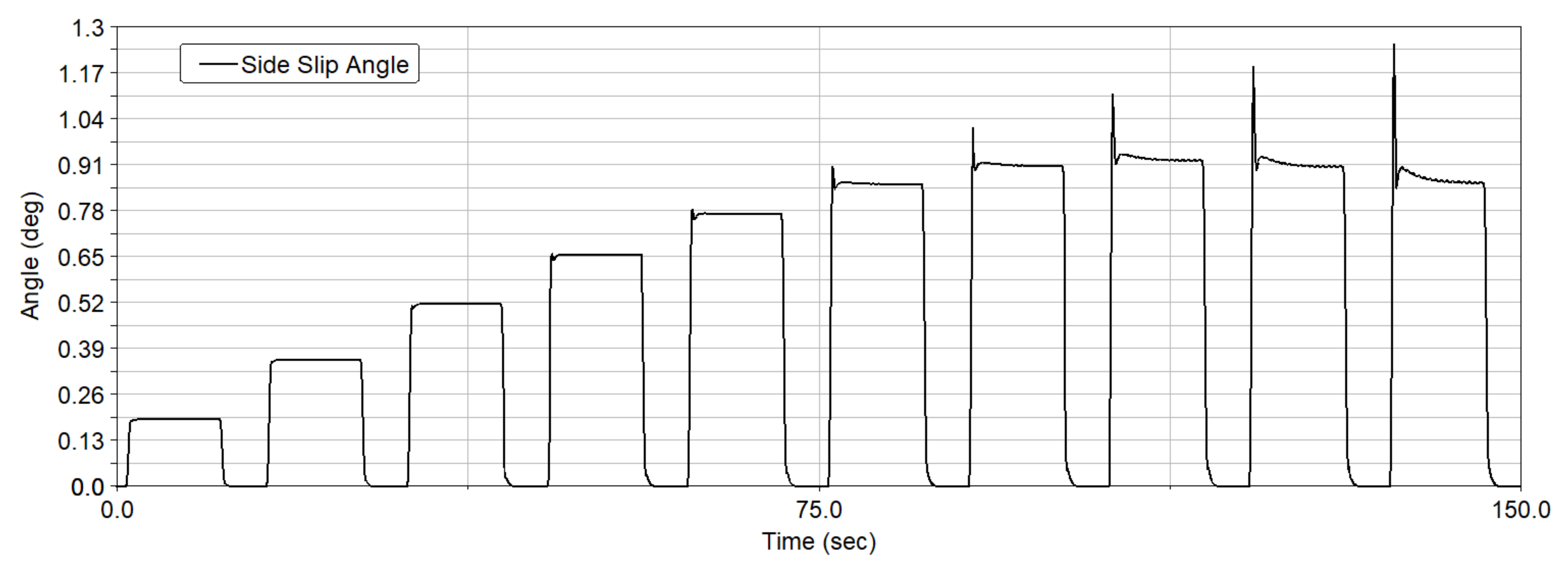
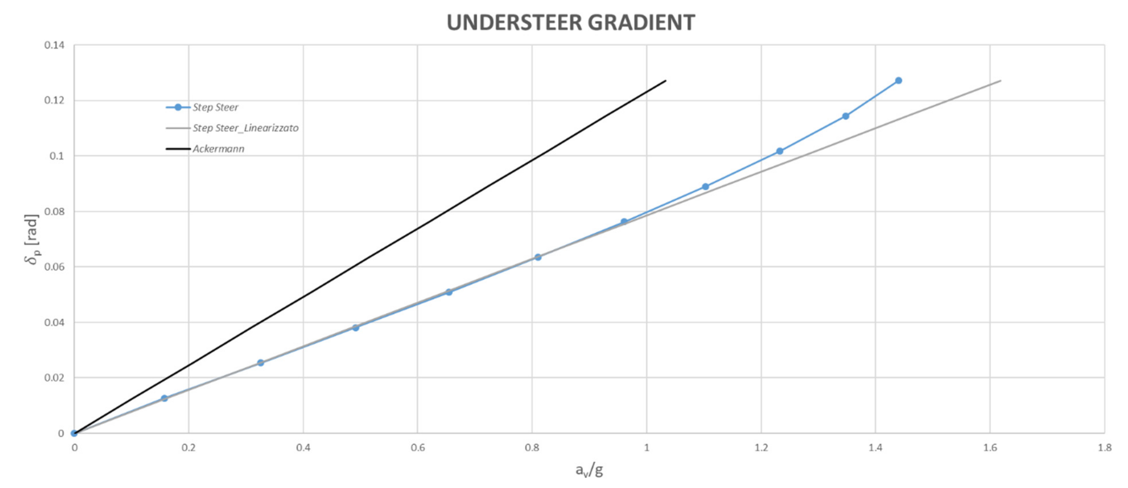
Once ${\tau }_s$ is defined, the understeer gradient can be evaluated by performing a set of step-steer maneuvers at constant speed (50 km/h) and increasing steering angle (ten successive steps of 0.07 rad (4°)). Figure 3 shows the input provided by the driver in terms of steering wheel and the corresponding vehicle output expressed as lateral acceleration (Figure 4) and slip angle (Figure 5). The steady-state vehicle response is measured for each step-steer maneuver using a “virtual” accelerometer. Results are collected in Figure 6 where the steady-state front steer angle is plotted against the normalized lateral acceleration. The understeer gradient can be directly estimated by Equation (6) that can be rearranged as:

$$K_{US}=\frac{d{\delta }_p}{d\left(\raisebox{1ex}{$a_y$}\!\left/ \!\raisebox{-1ex}{$g$}\right.\right)}-\frac{l g}{v^2}$$

(7)

where $v$ is the longitudinal speed. Therefore, $K_{US}$corresponds to the slope of the curve (0.0786 rad) minus the contribution related with the Ackermann steering angle (0.1232 rad) providing a final value of −0.0446 rad.

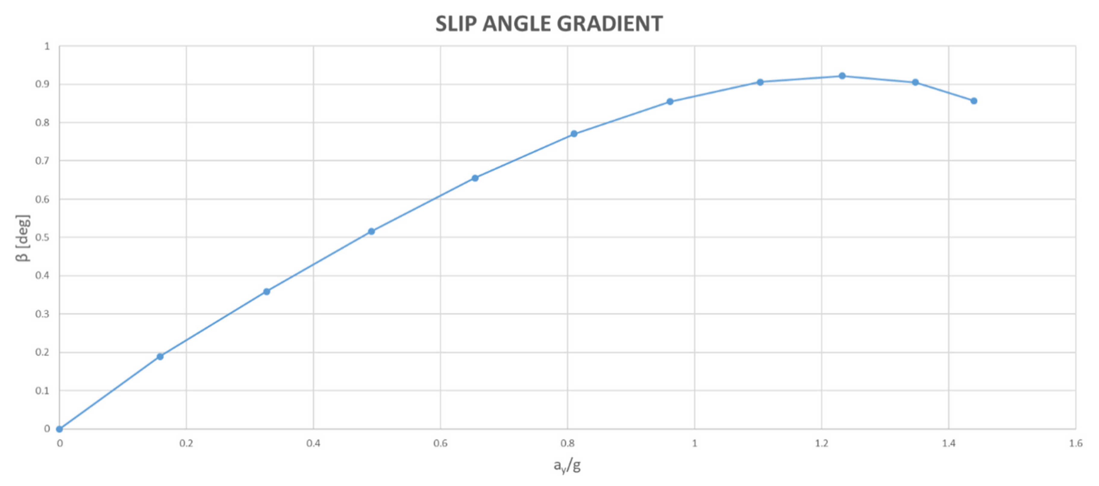
The car shows a tendency to a slight oversteer that is typical of sportive car with rear traction. A second parameter of interest is the gradient of the slip angle that is shown in Figure 7. It is consistent with the oversteer tendency. In general, the linear limit is rather high and close to 1 g. The vehicle exhibits a linear behavior with a loss of adhesion that is proportional to the track radius. The car can be considered as predictable and easy to control from the driver.

Finally, the parameters that can be typically adjusted to optimize the car performance are collected in the following

Table 2. Baseline configuration.

Baseline Set-Up	Front	Rear
Tire pressure	$\mathrm{70,000} \mathrm{Pa}$	$\mathrm{70,000} \mathrm{Pa}$
Camber angle	$0 \mathrm{rad}$	$0 \mathrm{rad}$
Toe-in	$0 \mathrm{rad}$	$0 \mathrm{rad}$
Anti-roll rocker height	$0.050 \mathrm{m}$	$0.050 \mathrm{m}$
Suspension spring stiffness	$\mathrm{61,294.4} \mathrm{N}/\mathrm{m} \left(350 \mathrm{lb}/\mathrm{in}\right)$	$\mathrm{61,294.4} \mathrm{N}/\mathrm{m} \left(350 \mathrm{lb}/\mathrm{in}\right)$
Suspension damper configuration	$C13 R13 \left(0-5/0-5\right)$	$C13 R13 \left(0-5/0-5\right)$
Brake balance	$62\%$	$38\%$

along with the nominal values that represent what is referred to as the baseline set-up throughout the paper. All remaining parameters of the car are fixed and cannot be adjusted without a substantial redesign of the vehicle that is not practical during a racing event. It is important to note that in all simulated test events the set-up parameters have been selected empirically through a grid-search approach that reflects as well as previous knowledge developed by the authors in vehicle handling dynamics and in Formula Student.

5. Set-Up Optimization

5.1. Tilt Test

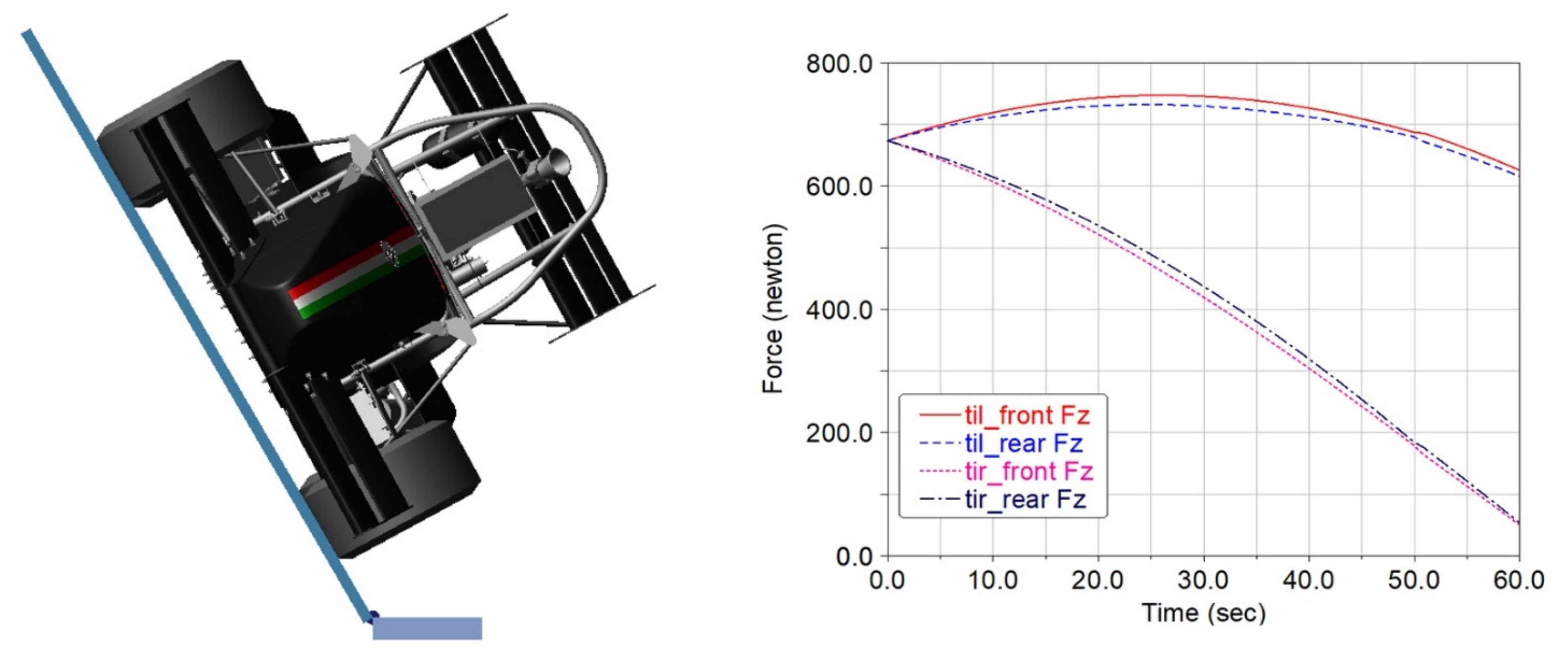
The objective of the Tilt Test in a FSAE contest is to verify if the car under investigation placed on a platform banked of 1.047 rad (60°) keeps contact with the supporting surface with all the four tires. The simulation is performed setting a lift velocity equal to 0.017 rad/s (1°/s), as stated in the regulation.

The test is positively passed if the normal component of the forces that the tires apply to the supporting surface is greater than zero for the whole duration of the simulation. Results are shown in Figure 8 where the final configuration of the car is on the left and the time history of the normal forces is shown on the right. As expected, at the beginning the tire vertical forces are equal. As the tilt angle increases, the tires of the external side (right side) unload up to a minimum value of about 44 N at the end of the test for the front right tire.

Therefore, the baseline set-up guarantees the successful fulfilment of the test without any adjustment. However, a possible regulation can be adopted to reach simultaneously the same normal force on both tires of the external side by operating on the front anti-roll bar system. Increasing the lever of 10% (e.g., up to 0.060 m), would lead to an increase in the normal force on both tires from 44 to 51 N with an increase of about 16%.

5.2. Brake Test

The second event of the FSAE competition refers to the Brake Test where the car is required to break by locking simultaneously the four tires with no significant deviation from the straight line while keeping the engine on. In order to simulate this test, four mini-events need to be defined as follows:

• Clutch—the driver inserts the clutch on and increases the engine rev:

  ⚬

  Throttle: step-like control, with a duration of $3 \mathrm{s}$, up to $100\%$;

  ⚬

  Braking: constant control, null value;

  ⚬

  Gear: constant control, first gear;

  ⚬

  Clutch: constant control, unitary value;

  ⚬

  Conditions: stop when $rp{m}_{engine}\gg 6450 \mathrm{rpm}$.

• Release—the driver releases the clutch at the right engine rev:

  ⚬

  Throttle: constant control, relative null value;

  ⚬

  Braking: constant control, null value;

  ⚬

  Gear: constant control, first gear;

  ⚬

  Clutch: step-like control, duration $0.1 \mathrm{s}$, up to $0\%$;

  ⚬

  Conditions: terminate when $time=0.1 \mathrm{s}$.

• Acceleration_1Gear—the driver releases the clutch and accelerates:

  ⚬

  Throttle: relative step like control, duration of 0.5 s, up to 100%;

  ⚬

  Braking: constant control, null value;

  ⚬

  Gear: constant control, first gear;

  ⚬

  Clutch: constant control, null value;

  ⚬

  Conditions: terminate when $velocity>65.7 \mathrm{km}/\mathrm{h}$.

• Braking—the driver performs emergency braking:

  ⚬

  Throttle: step-like control, duration of 0.5 s, up to 0%;

  ⚬

  Braking: step-like control, starts at $0.5 \mathrm{s}$, duration of $0.2 \mathrm{s}$, up to $100\%$;

  ⚬

  Gear: constant control, first gear;

  ⚬

  Clutch: step-like control, duration of $0.5 \mathrm{s}$, up to unitary value;

  ⚬

  Conditions: terminate when $velocity<0.36 \mathrm{km}/\mathrm{h}$.

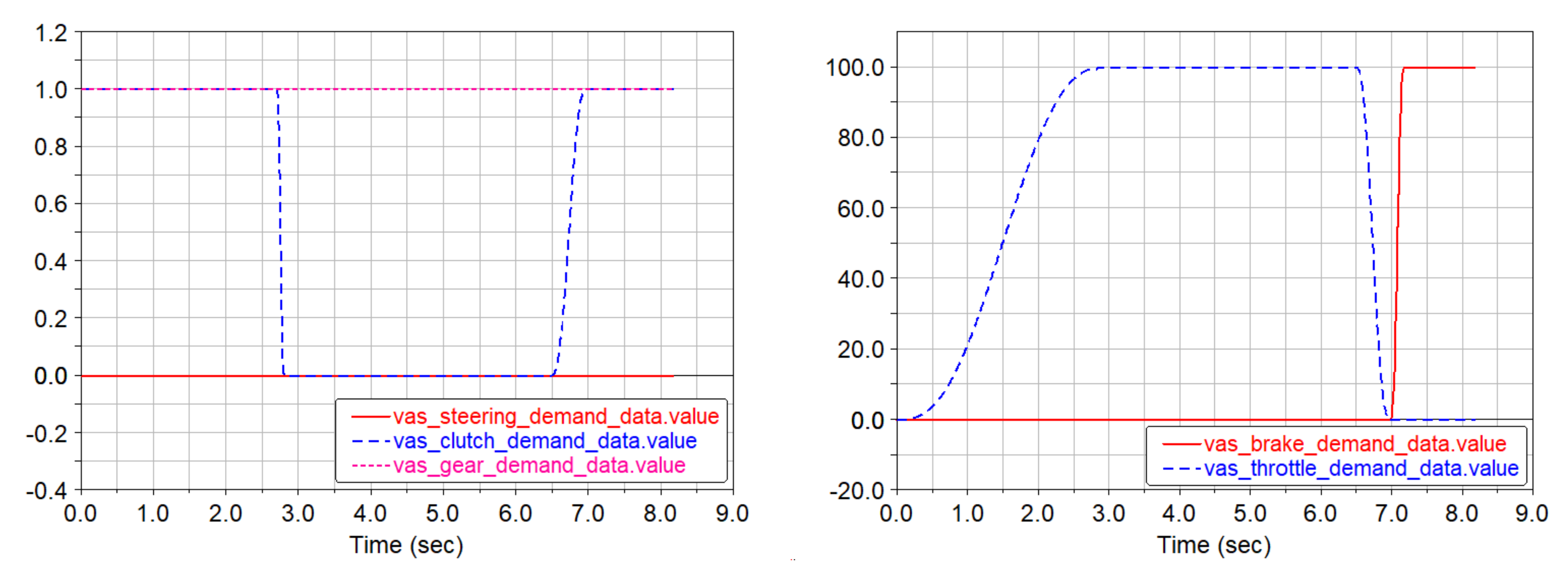
In order to better understand the four mini-events, Figure 9 shows the time history of the driver input in terms of steering wheel, clutch, and gear demand (left side), acceleration and braking (right side).

The track for the brake test is 95 m long with a friction coefficient of 0.75 (as suggested by the tire datasheet) that simulates the non-ideal contact between a “cold” tire and a standard asphalt. This value is far from the ideal condition of unitary friction coefficient (optimal contact between tire and the road drum in a single-wheel test bed).

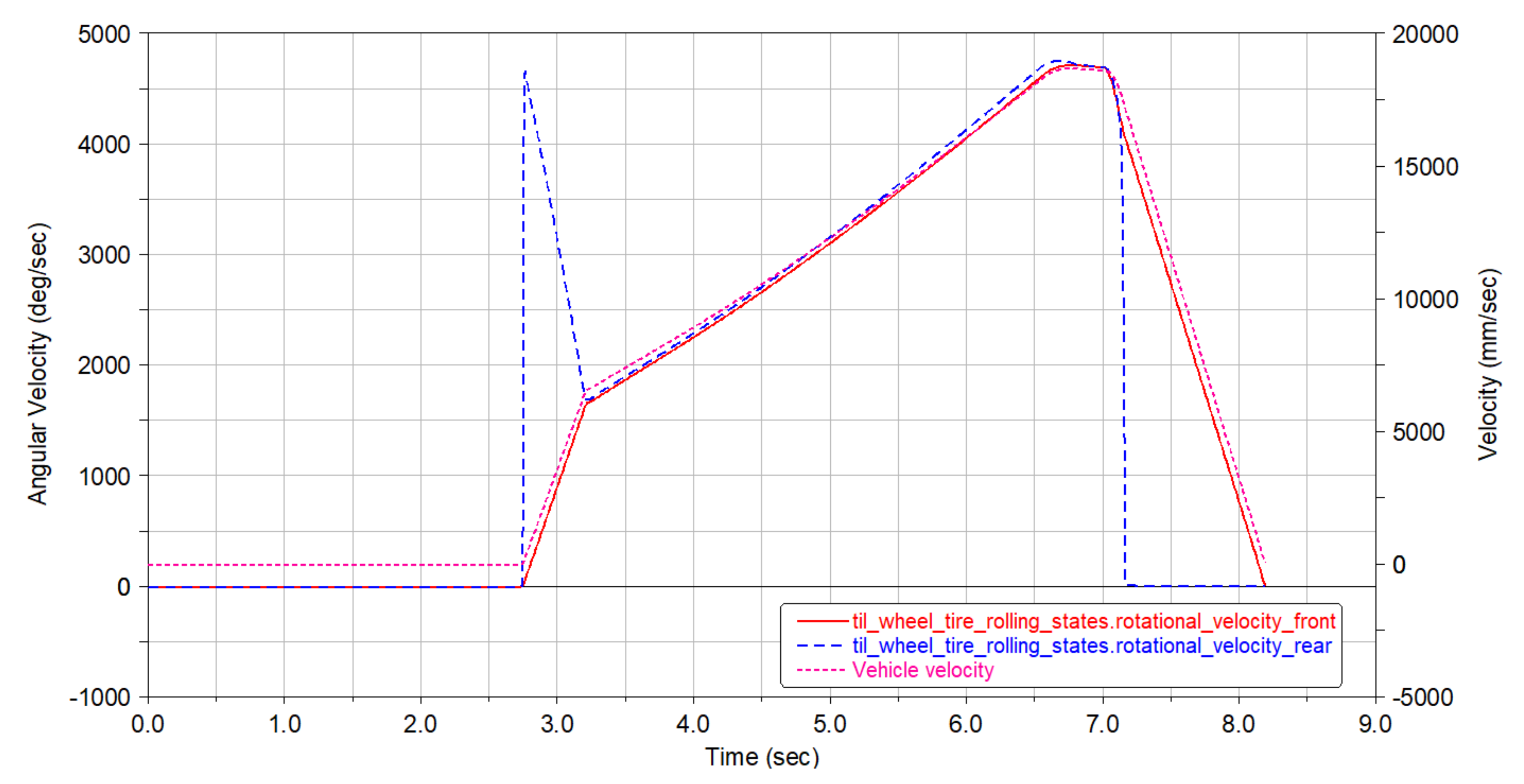
The objective in this test is to lock the four tires before the car reaches a full stop. In Figure 10, the tire angular velocity (left y-axis) is plotted as a function of time against the car velocity (right y-axis). For simplicity, only the tires of the left side are reported. Focus is given to the final part of the braking test.

Using the baseline set-up, the test fails as the front tires do not lock, whereas the rear tires lock at about 7 s. In order to reach simultaneous lock of all four tires, the friction of the front wheels need to be reduced. This objective can be achieved by

• Increasing inflation pressure to reduce the tire contact patch;
• Increase the camber angle to reduce the tire contact patch;
• Increase brake balance to compensate for weight shift during braking.

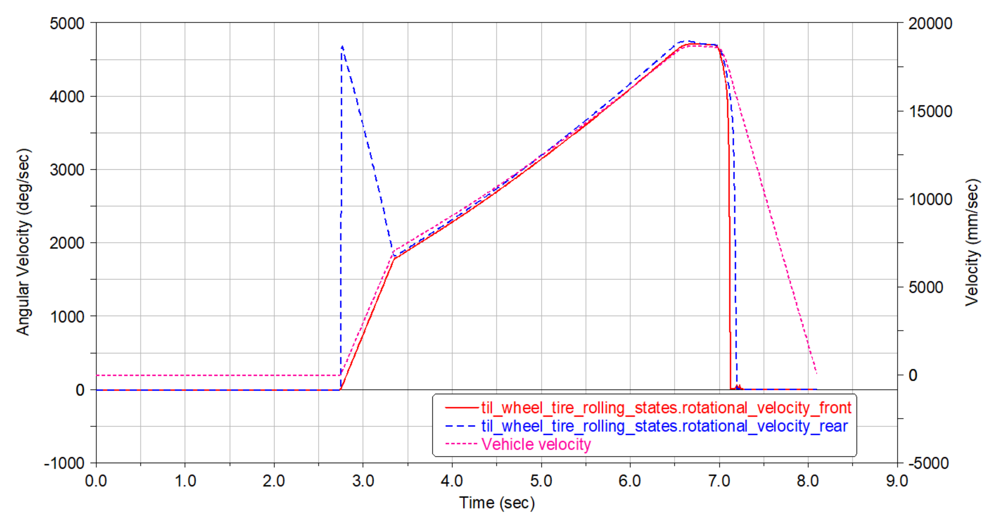
First two steps need to be performed on both rear and front wheels so that shifting the brake balance towards the front prevent rear tires to lock up. The optimized set-up that leads to all tire lock-up, as shown in Figure 11, results as follows

• Front/rear inflation pressure: $\mathrm{100,000} \mathrm{Pa}$
• Front/rear camber angle: $-0.043 \mathrm{rad} \left(-2.5°\right)$
• Front braking balance: $74\%$

5.3. Acceleration Event

The Acceleration Event is a longitudinal acceleration test with the car starting from rest and driving along a straight of 75 m. In order to simulate the event, four mini-events need to be created keeping the steering angle null.

• Clutch—the driver inserts the clutch on and increases the engine rev:

  ⚬

  Throttle: step-like control, duration $3 \mathrm{s}$, up to $100\%$;

  ⚬

  Braking: constant control, null value;

  ⚬

  Gear: constant control, first gear;

  ⚬

  Clutch: constant control, unitary value;

  ⚬

  Conditions: terminate when $rp{m}_{engine}\gg 6450 \mathrm{rpm}$.

• Release—the driver releases the clutch:

  ⚬

  Throttle: constant control, relative null value;

  ⚬

  Braking: constant control, null value;

  ⚬

  Gear: constant control, first gear;

  ⚬

  Clutch: step-like control, duration $0.1 \mathrm{s}$, up to $0\%$;

  ⚬

  Conditions: terminate when $time=0.1 \mathrm{s}$.

• Acceleration_1Gear—the driver accelerates up to 100%:

  ⚬

  Throttle: relative step-like control, duration of $0.5 \mathrm{s}$, up to 100%;

  ⚬

  Braking: constant control, null value;

  ⚬

  Gear: constant control, first gear;

  ⚬

  Clutch: constant control, null value;

  ⚬

  Conditions: terminate when $rp{m}_{engine}\gg 4000 \mathrm{rpm}$.

• Acceleration—the driver keeps accelerating:

  ⚬

  Throttle: constant control, up to $100\%$;

  ⚬

  Braking: constant control, null value;

  ⚬

  Gear: machine-type control;

  ⚬

  Clutch: machine-type control;

  ⚬

  Conditions: terminate when $distance\gg 75 \mathrm{m}$.

In order to better understand the set of mini-events, Figure 12 shows the driver input in terms of steering demand, clutch, and gear (left side) and accelerator and brake (right side) as a function of time.

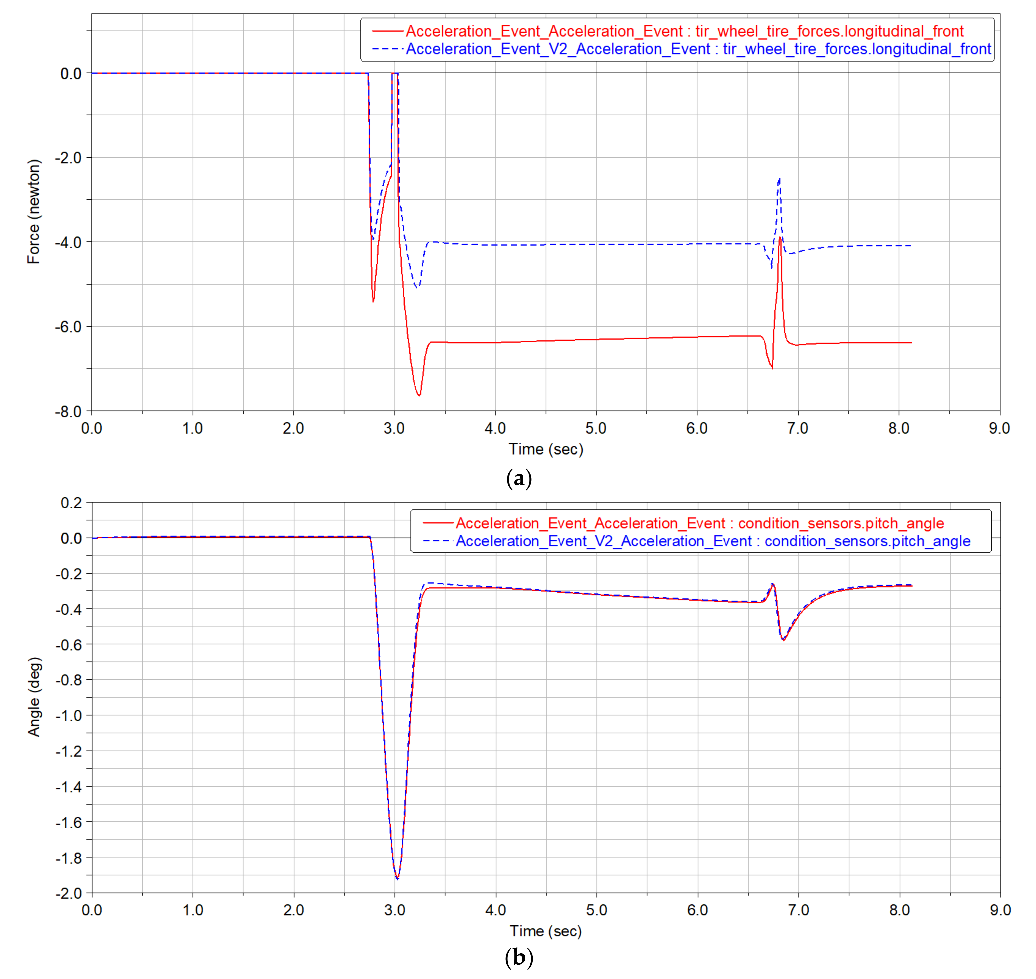
The road type is the same of that used for the Brake Test. The objective is to drive the 75 m long straight with the best time as recorded between two photocells, one placed at the finish line and the other at 0.3 m from the start line. Other parameters of interest for this test are the pitch angle and the longitudinal acceleration of the chassis.

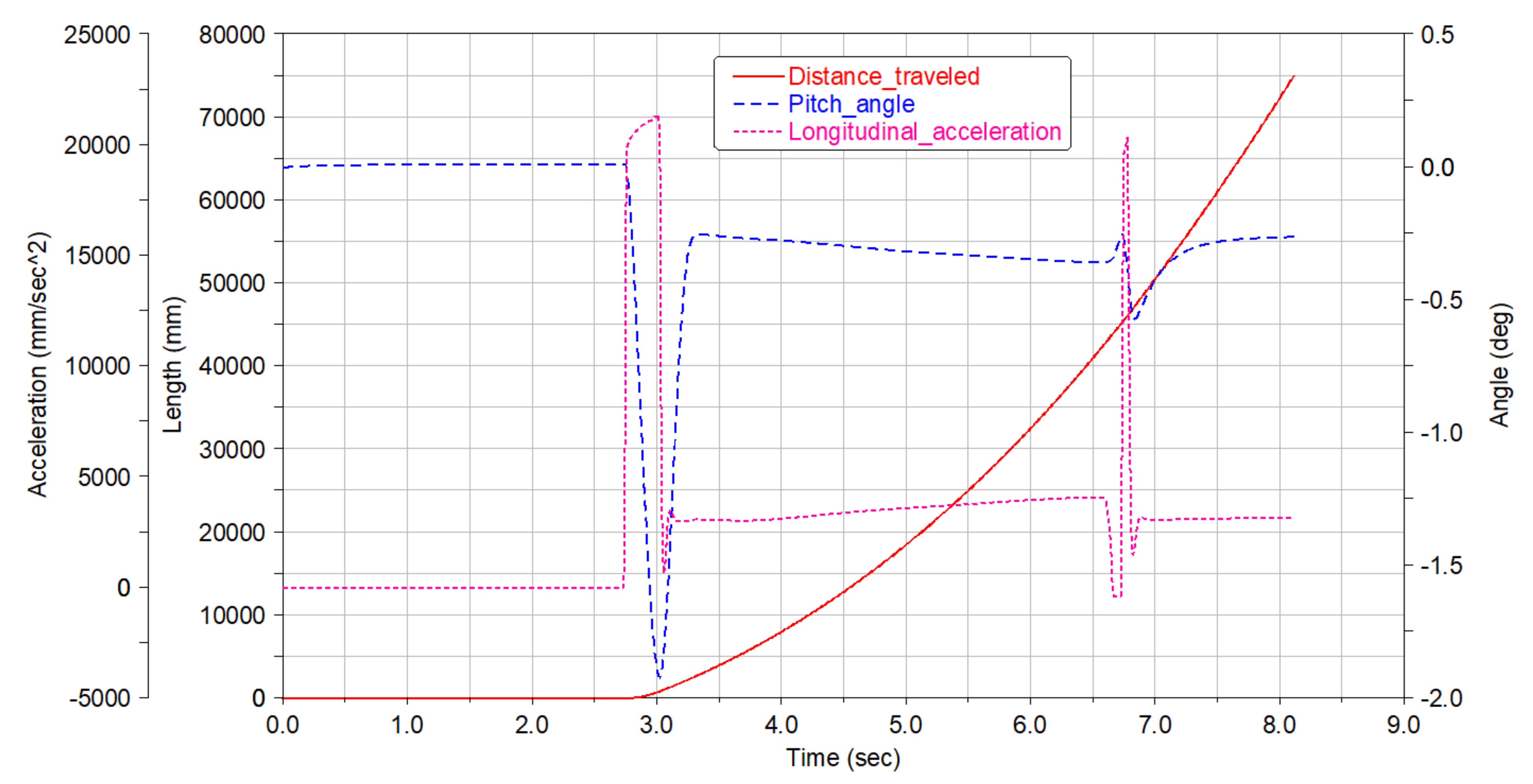
In Figure 13, the travelled distance is plotted in red indicating a time required to cover the two regulation points of 5.21 s. From the longitudinal acceleration curve in blue and chassis pitch angle, it is apparent when the clutch is released (positive peak of acceleration and negative of pitch) at about 3 s. Afterwards, the car follows a uniformly accelerated motion with 0.4 g acceleration. The pitch motion is underdamped and stabilizes around a value of about −0.005 rad (−0.29°).

When the 7th second is reached, the second gear is shifted with a similar transient behavior. In this test, to optimize the car performance during acceleration, the ability of the drive rear tires to develop longitudinal adhesion need to be increased whereas that of front tires (free rolling) need to be reduced. This can be achieved by regulating the following parameters:

• Inflation pressure higher for the front tires to reduce the contact patch;
• Camber angle larger for the front tires to reduce the contact patch;
• Softer anti-roll spring stiffness to the rear to increase the elastic-type weight shift on the rear drive tires.

The final configuration resulted in:

• Front inflation pressure: $\mathrm{100,000} \mathrm{Pa}$
• Front camber angle: $-0.043 \mathrm{rad} \left(-2.5°\right)$
• Rear spring stiffness: $\mathrm{43,800} \mathrm{N}/\mathrm{m}\left(250 \mathrm{lb}/\mathrm{in}\right)$

However, the time reduction is small and almost negligible from 5.21 to 5.19 s. This confirms the good trade-off of the baseline configuration (denoted by a red line) that is compared with the optimized set-up (blue line) in Figure 14. The baseline configuration can be hardly improved as showed in Figure 14a where although the relative reduction in the motion resistance compared to the optimized set-up is of 40%, it corresponds to only 3 N in absolute terms.

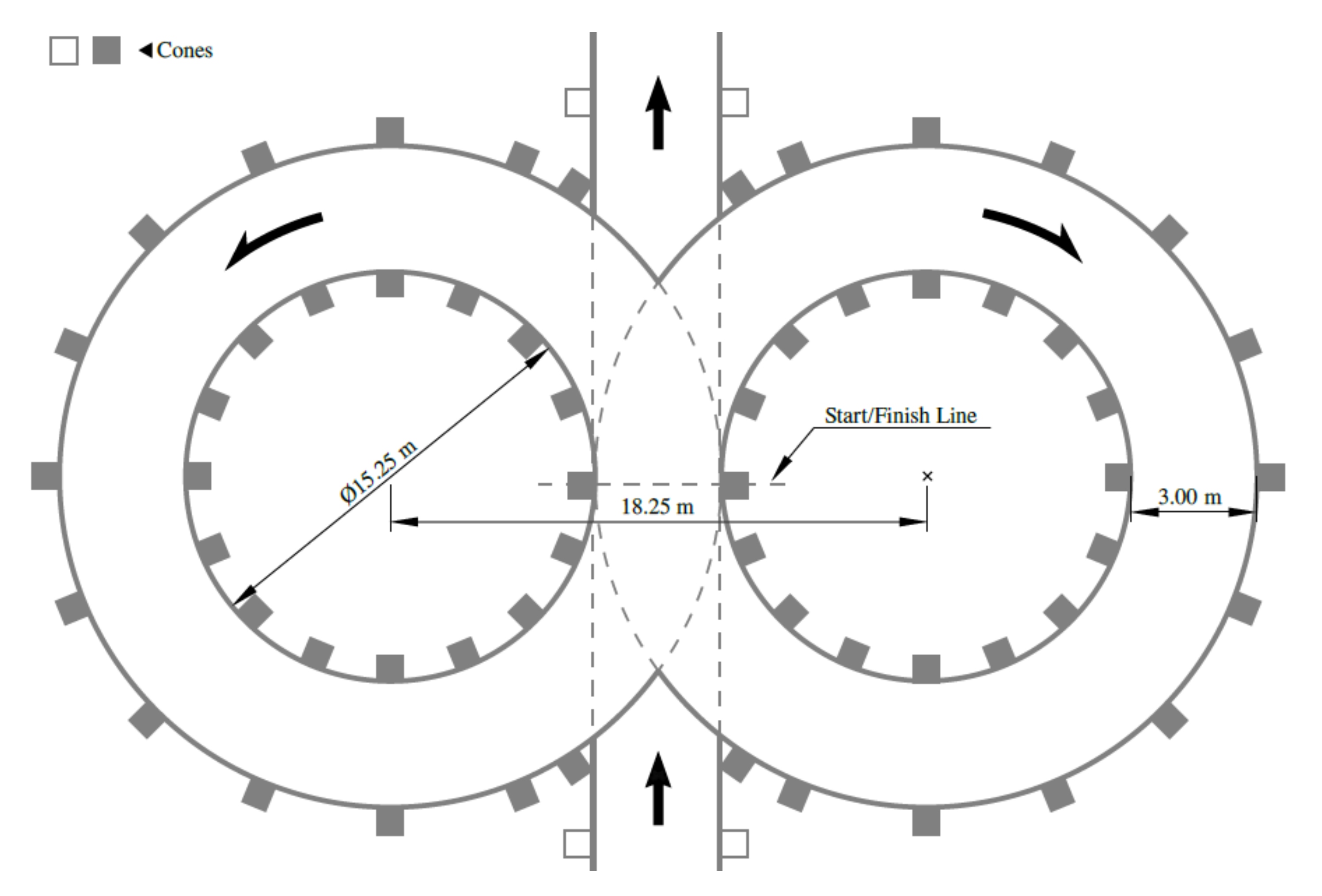
5.4. Skidpad Event

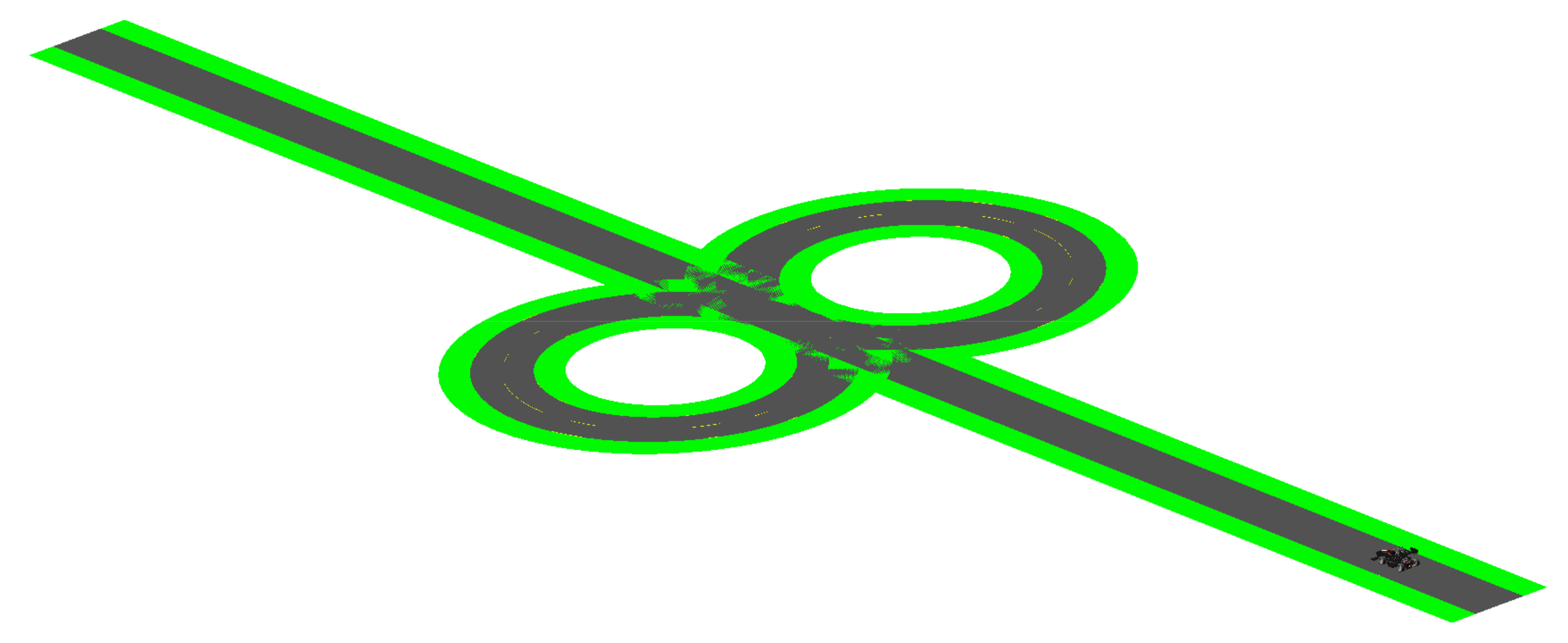
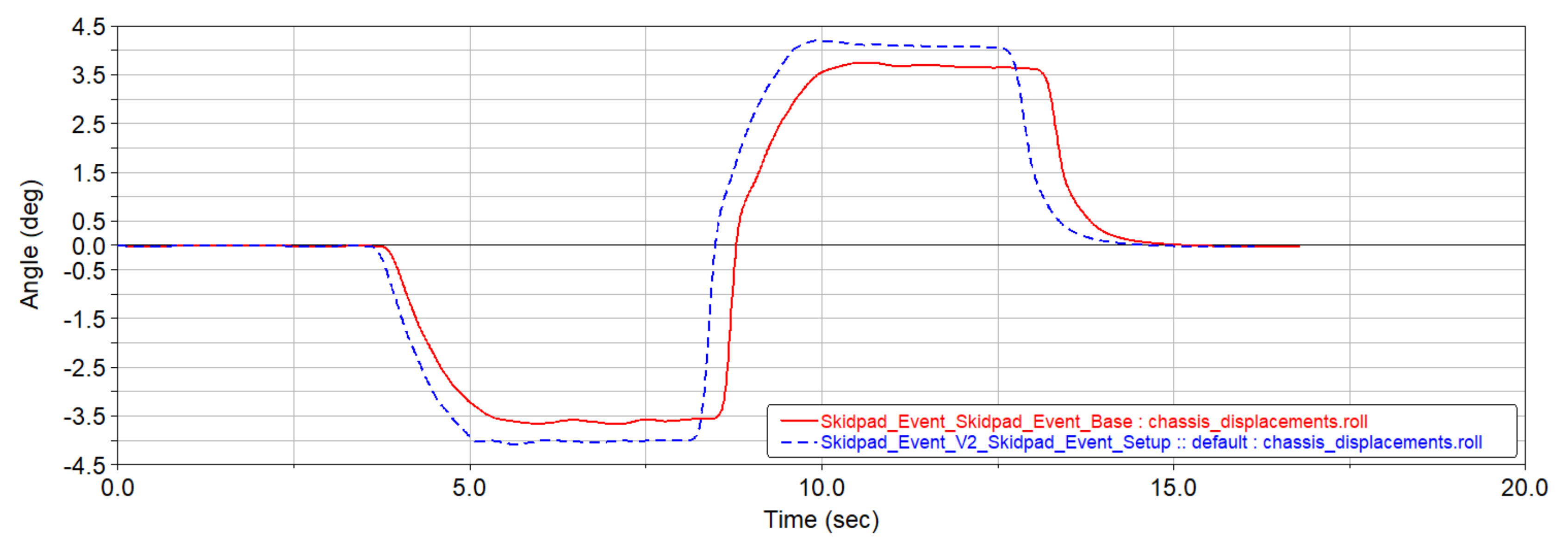
Finally, the Skidpad Event is discussed, where the car is required to follow an eight-shaped track as shown in Figure 15.

In contrast to previous simulations, here the driver is required to control both the steering wheel to track the road and the acceleration level to keep the correct limit speed during turning motion. A single mini-event is required, so defined:

• Skidpad—the driver tracks the optimal trajectory:

  ⚬

  Steering: machine-type control based on a predefined trajectory in the form of a point set or “path map”;

  ⚬

  Throttle/Braking: machine-type control to maintain the initial speed constant;

  ⚬

  Gear: relative constant control, null value;

  ⚬

  Clutch: relative constant control, null value;

  ⚬

  Conditions: terminate when $distance\gg 210 \mathrm{m}$

Before and after the track defined by regulation, two 50 m straights have been added to allow the vehicle to reach steady-state conditions, as shown in Figure 16.

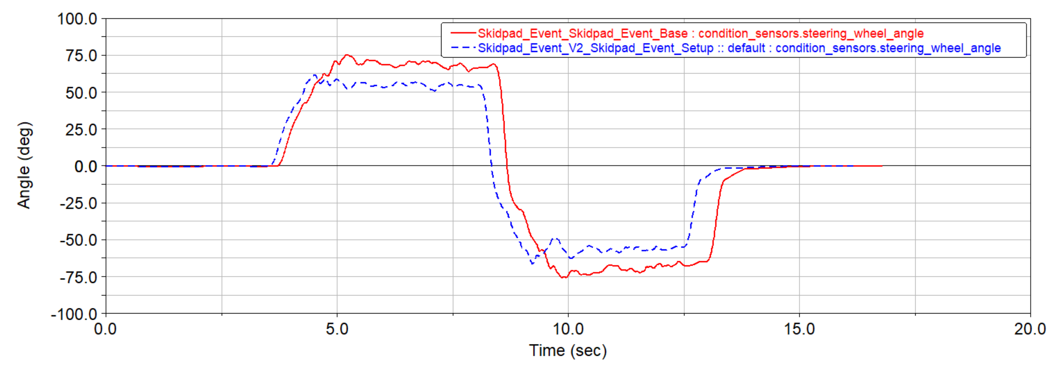
First, the vehicle tuned with the baseline set-up is evaluated. It is found a maximum speed of 45 km/h before directional instability occurs. The lap time is measured for the first circle since it easier to detect the two times when the car crosses the photocell line.

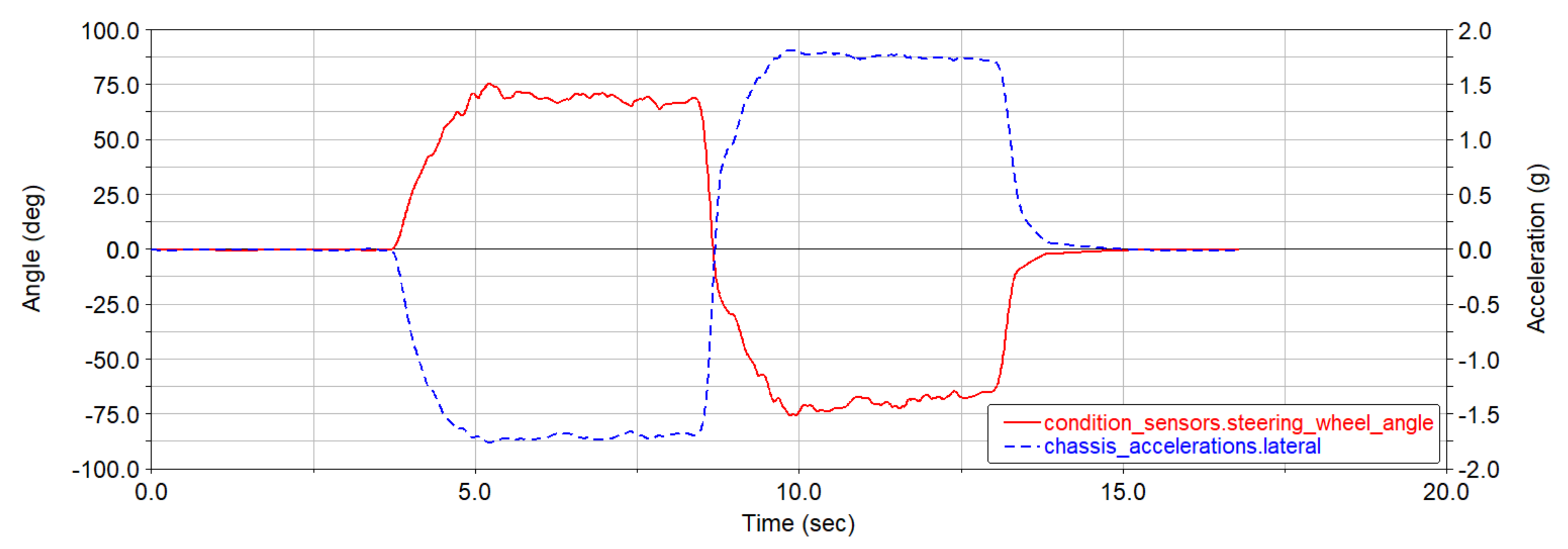
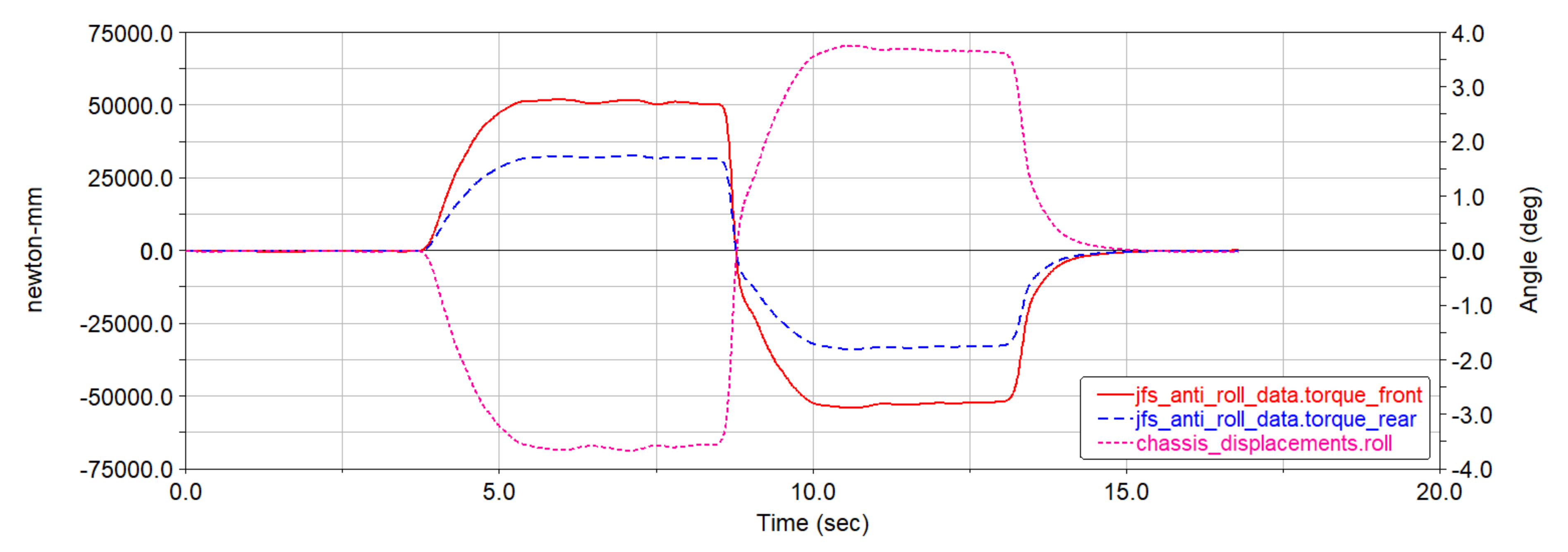
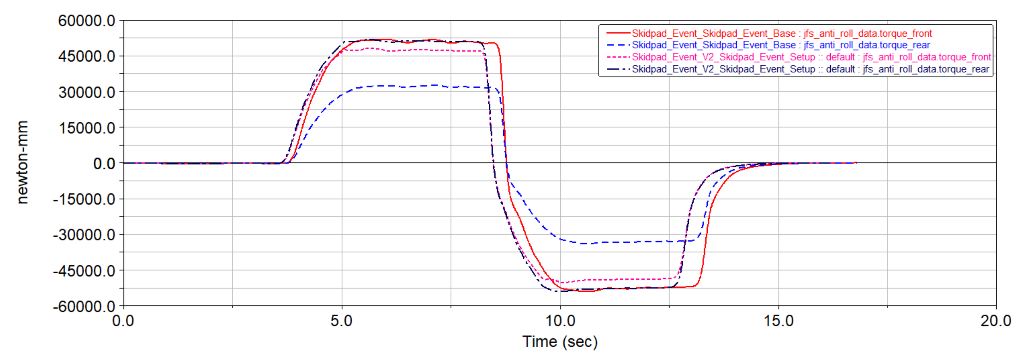
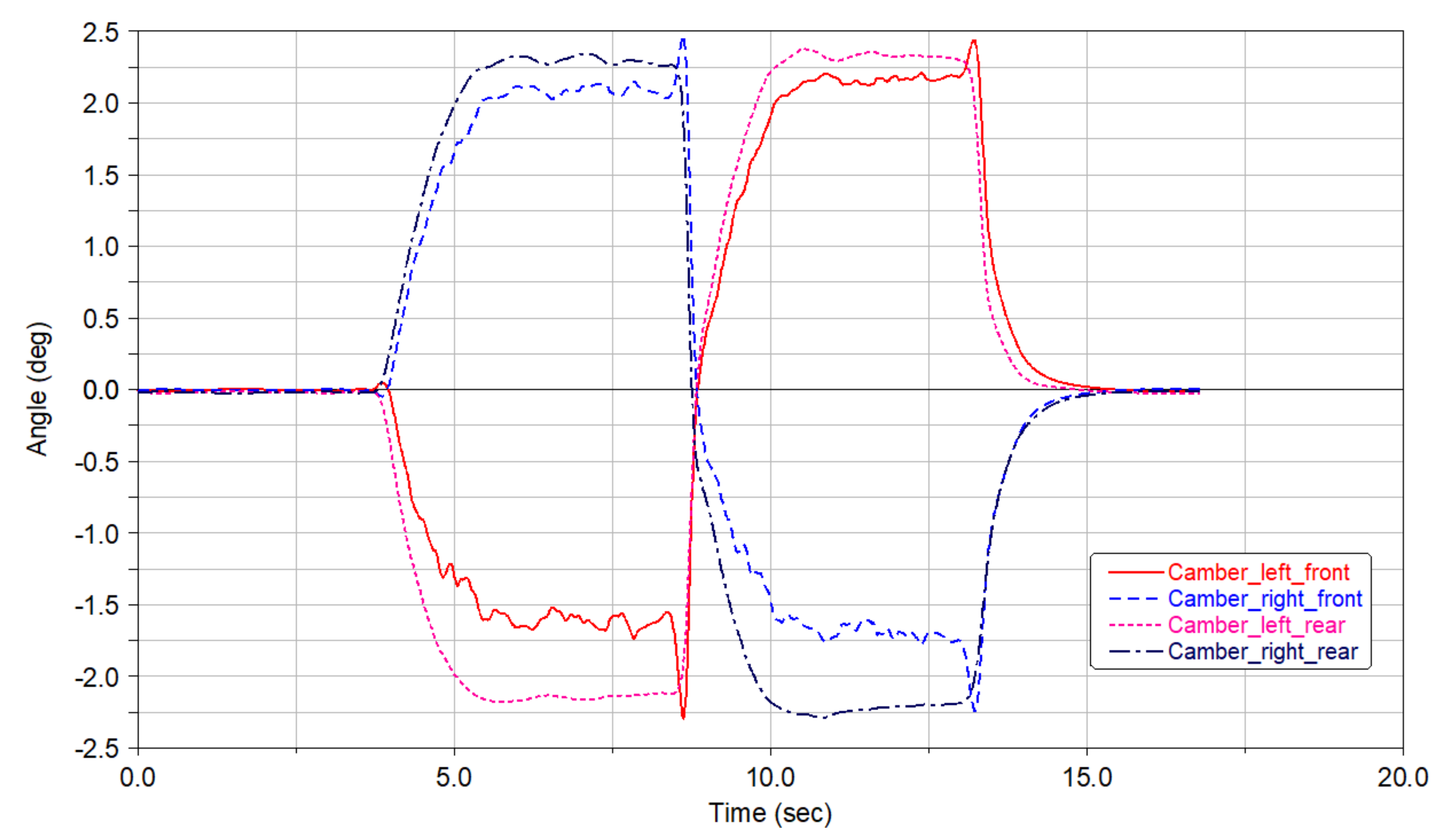
Many parameters can be evaluated. For example, the steering angle and the lateral acceleration as shown in Figure 17. The roll angle and the corresponding spring roll torque provided by the anti-roll system are shown in Figure 18. Finally, the camber angle for all tires is reported in Figure 19 suggesting the main parameter that can be adjusted to improve the ability of tires to exchange forces with the road.

Using the baseline set-up, the first round of the track is travelled in about 4.98 s. The average value of the lateral acceleration is about 1.7 g that is consistent with the maximum adhesion values of these tires.

One approach to increase the lateral adhesion is to operate on the camber angle of the tires. It can be seen from Figure 19 that the external tires (e.g., the right-side tires being the first round driven in counter-clockwise direction) show a positive increase in the camber angle of about 0.038 rad (2.2°); therefore, a static camber angle of equal and opposite value is adopted. Since they hold most of the disturbance lateral force, the handling response will be generally improved. The outer tires bear most of the normal force due to the lateral weight transfer and they develop larger lateral forces. During clockwise driving, the situation is inverted but again the external tires play the critical role. The static camber angles depend as well as on the regulation of the anti-roll system since its variation depends on the kinematic behavior of the car as a function of the roll angle of the chassis.

By stiffening the anti-roll bars, the roll angle can be reduced. It can be seen from Figure 18 that the roll angle results in about 0.062 rad (3.55°) for the baseline configuration. In contrast, the final optimized configuration is:

• Front/rear camber angle: $-0.043 \mathrm{rad} \left(-2.5°\right)$
• Front anti-roll bar height: $0.065 \mathrm{m}$
• Rear anti-roll bar height: $0.035 \mathrm{m}$

The time to complete the first round is 4.76 s, with a limit velocity equal to 46.8 km/h leading to a reduction of about 5% in the test time.

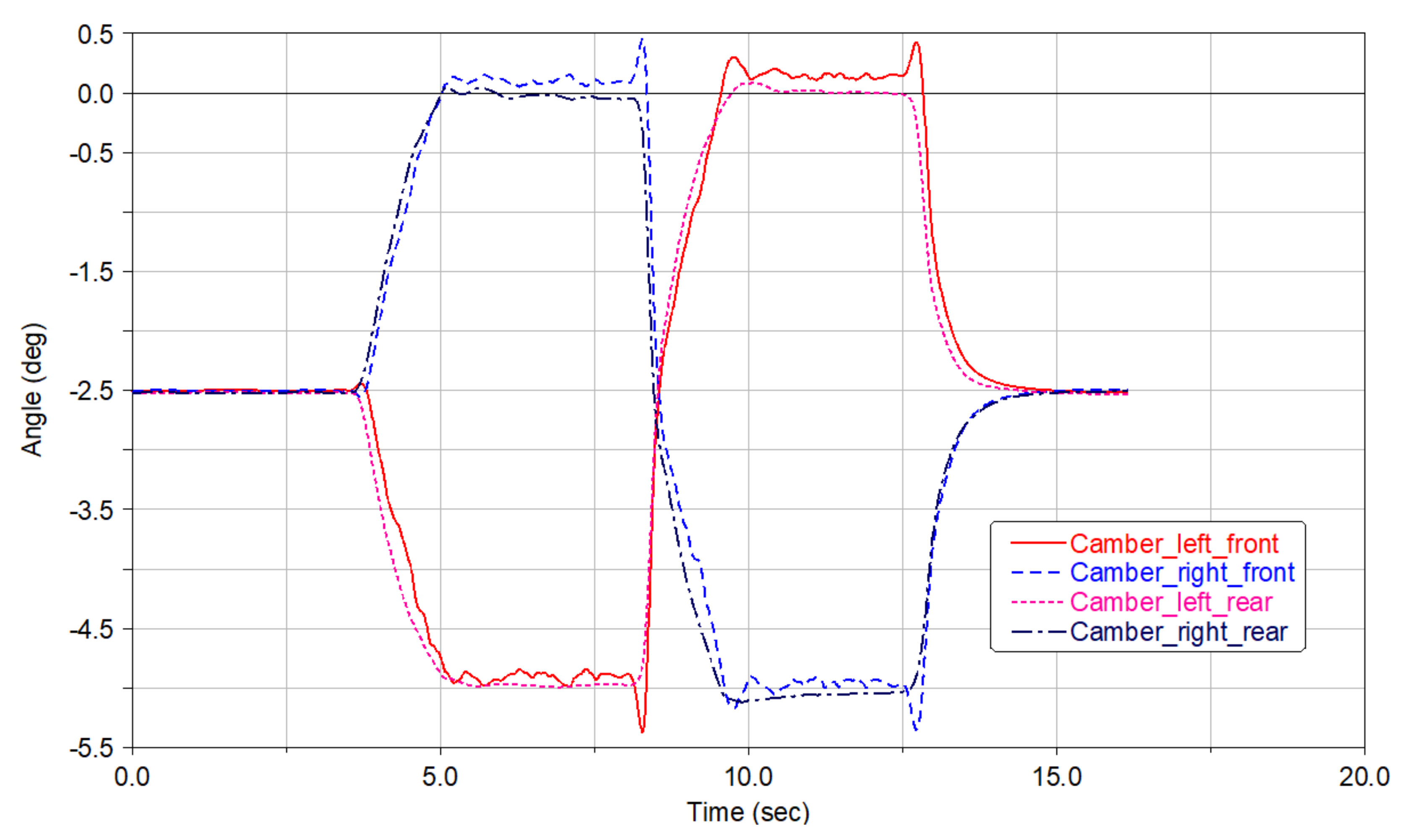
The optimal value of the static camber angle (equal to −2.5°) was chosen in order to obtain the maximum contact patch during turning motion (Figure 20). This in turn leads to a larger roll angle of the chassis (Figure 21).

Note that the antiroll bar was stiffened to the rear and soften at the front to avoid the lift of the internal front tire (Figure 22).

Some interesting conclusions can be drawn from the analysis of the handling response. The lateral acceleration increases up to 1.85 g that is directly related to the larger vehicle speed. The maximum steering wheel decreases from 1.3 rad (74.5°) to 1.09 rad (62.5°) (Figure 23).

This can be explained when considering that the vehicle exhibits an oversteer behavior that allows the car to drive the same circular trajectory with less steering angle for increasing speed.

5.5. Discussion and Lessons Learnt

To summarize, the parameters of the baseline configuration and the values to be replaced in each test event to gain performance improvement of the Formula Student car are collected in

Table 3. Baseline contrasted with fine-tuned setups.

Baseline Set-Up	Front	Rear
Tire pressure	$\mathrm{70,000} \mathrm{Pa}$	$\mathrm{70,000} \mathrm{Pa}$
Camber angle	$0 \mathrm{rad}$	$0 \mathrm{rad}$
Toe-in	$0 \mathrm{rad}$	$0 \mathrm{rad}$
Anti-roll rocker height	$0.050 \mathrm{m}$	$0.050 \mathrm{m}$
Spring stiffness	$\mathrm{61,294.4} \mathrm{N}/\mathrm{m} \left(350 \mathrm{lb}/\mathrm{in}\right)$	$\mathrm{61,294.4} \mathrm{N}/\mathrm{m} \left(350 \mathrm{lb}/\mathrm{in}\right)$
Damper configuration	$\mathrm{C}13 \mathrm{R}13 \left(0-5/0-5\right)$	$\mathrm{C}13 \mathrm{R}13 \left(0-5/0-5\right)$
Brake balance	$62\%$	$38\%$
Set-Up Tilt Test	Front	Rear
Anti-roll rocker height	$0.060 \mathrm{m}$	$0.050 \mathrm{m}$
Set-Up Brake Test	Front	Rear
Tire pressure	$\mathrm{100,000} \mathrm{Pa}$	$\mathrm{100,000} \mathrm{Pa}$
Camber angle	$-0.043 \mathrm{rad} \left(-2.5°\right)$	$-0.043 \mathrm{rad} \left(-2.5°\right)$
Brake balance	$74\%$	$26\%$
Set-Up Acceleration Event	Front	Rear
Tire pressure	$\mathrm{100,000} \mathrm{Pa}$	$\mathrm{70,000} \mathrm{Pa}$
Camber angle	$-0.043 \mathrm{rad} \left(-2.5°\right)$	$0 \mathrm{rad}$
Spring stiffness	$\mathrm{61,294.4} \mathrm{N}/\mathrm{m} \left(350 \mathrm{lb}/\mathrm{in}\right)$	$\mathrm{43,800} \mathrm{N}/\mathrm{m} \left(250 \mathrm{lb}/\mathrm{in}\right)$
Set-Up Skidpad Event	Front	Rear
Camber angle	$-0.043 \mathrm{rad} \left(-2.5°\right)$	$-0.043 \mathrm{rad} \left(-2.5°\right)$
Anti-roll rocker height	$0.065 \mathrm{m}$	$0.035 \mathrm{m}$

.

As seen from this table, fine-tuning of the baseline set-up can substantially help the car to fulfill and exceed the target set by the specific test. When the tilt contest is considered, the same vertical load can be achieved on the tires of the external side by increasing the stiffness of the front anti-roll bar system. This regulation directly impacts on the front/rear weight distribution due to a lateral disturbance force, e.g., the weight force component in this case.

One of the challenges in the brake test is to lock simultaneously front and rear tires. However, front tires tend to lock less than rear ones. This tendency can be corrected by operating on both the tires (camber angle and inflation pressure) and the car braking system. The increase in the brake balance helps to compensate for the longitudinal weight shift during braking, whereas the tire adhesion can be reduced on all wheels via a larger pressure and camber angle. Both parameters contribute to decrease tire adhesion by reducing the contact patch [23].

Similarly, to maximize acceleration of a Formula Student car, the adhesion of the rear tires must be increased whereas that of the free rolling front tires should be kept as low as possible. Again, this objective can be achieved by increasing the inflation pressure and the camber angle on the front tires (smaller tire footprint) in combination with a softer anti-roll bar spring on the rear that increases the corresponding elastic-type weight shift.

Finally, if the skidpad event is targeted one approach to gain a larger lateral adhesion and so a higher corner velocity is to operate with the tires perfectly perpendicular to the road. Attention should be given especially to the external wheels that are those that mostly contribute to balance the centrifugal force during turning motion. By fine-tuning the static camber angles and the stiffness of the anti-roll systems, the change in the camber angle of the external tires in their compression travel with respect to the chassis can compensate the roll angle and keep the tires flat on the road. In this case, the maximum travel velocity can be improved of about 2 km/h.

6. Conclusions

This paper presented a comprehensive multi-body approach to virtual prototyping of formula car that aims at the dynamic characterization of a full-car assembly and to its performance optimization. The described approach allows one to evaluate the performance of the car and the impact of the many adjustable parameters that defines its set-up and that allows for a fine-tuning of the whole systems. Multi-body modeling and simulation is a powerful tool available to the modern engineers to analyze and understand the complex underlying mechanisms that govern the full-car response prior to any expensive and time-consuming track testing.

Future developments of this research include the validation of the multi-body model against real track tests performed using the Formula SAE prototype currently in the final stage of construction. The comparison of the experimental results with those obtained from the simulations is a key element to validate the whole concept.