1. Introduction
Nowadays, robots are increasingly asked to work in unstructured environments. In many cases, they are supported by sensor-based safety systems, avoiding fences that typically isolate the cell workspace within the workshop. Moreover, the trend toward collaborative robotics portends to a workshop layout where robots and humans share the workspace and collaborate in many operations, in a dynamical and unforeseeable scenario. In addition to dedicated hardware and design principles, collaborative robotics implies specific control strategies to ensure safety [
1,
2]. In this sense, collision avoidance control techniques represent a powerful means of improving the safety and flexibility of robots. A number of papers are available in the literature on path planning and obstacle avoidance for mobile robots [
3], which is a very common problem. A more complex problem is the collision avoidance for industrial manipulators, which suffer from the limitations of the workspace and problems of singularity. In this case, redundant manipulators offer greater dexterity than traditional manipulators, which aids in the development of task-oriented control strategies taking advantage of the additional degrees of freedom. Thus, redundant manipulators are the best candidates for high dexterity tasks with collision avoidance capability [
4,
5]. Moreover, redundancy can also be exploited with standard manipulators if some of the degrees of freedom of the end-effector, e.g., the orientation angles, can be kept free during motion.
Thus, an overall control strategy for a manipulator working in a dynamic environment can be conceived as the combination of:
An off-line path planning algorithm, which plans the trajectory of the robot’s end-effector taking into account the possible presence of disturbing obstacles, modifying the path based on the positions of the obstacles before the motion starts;
An on-line motion control algorithm, which controls in real-time the robot compensating for obstacles that are moving, or new obstacles entering the workspace;
A redundancy control strategy that exploits the dexterity of the manipulator to avoid collisions between obstacles and the kinematic chain of the manipulator;
A robust technique for the avoidance of singular configurations during motion.
Dealing with motion planning for obstacle avoidance, several methods are available in the literature [
6], such as Rapidly-exploring Random Trees (RRT) [
7,
8], grid-based algorithms [
9,
10] or Batch Informed Trees (BIT) and Model Predictive Control (MPC) [
11]. A very common approach consists in defining artificial potential fields, which drive the robot to the target inside the workspace [
12,
13,
14]. The result of the potential fields is a set of forces, attractive toward the goal and repulsive from the obstacle regions. Typically, such forces are associated with velocities applied to the end-effector of the manipulator; then, the trajectory can be obtained by numerical integration.
A further problem in optimal path planning for automation and robotics is the generation of smooth trajectories: an optimal algorithm for trajectory generation must guarantee smoothness in terms of position and velocity to be implemented in the controller of a real system. The use of smooth curves, e.g., the Bézier curves, can help solve this problem, as proposed by the authors in [
15]: several examples of applications can be found in different fields, such as automated vehicle guidance [
16,
17], aerial autonomous vehicles [
18] or spherical parallel manipulators [
19,
20].
The same principle of repulsive velocities generated by obstacles can be used to avoid collisions between obstacles and control points along the kinematic chain of the manipulator: in addition to the motion imposed to end-effector, a repulsive velocity vector can be applied to the point of the robot that is closer to one of the obstacles, adding a task to the control system [
21,
22]. Such an approach is typically applied to redundant manipulators [
23,
24], where additional tasks can be assigned maintaining the trajectory of the end-effector. Furthermore, the entity of the repulsive velocity can be thought in general as a function of several parameters besides obstacle/robot positions, e.g., the relative speed [
25] or other energetic criteria [
26].
The authors studied this kind of approach in [
15] for a planar case; in addition to the standard method, a modified repulsive velocity was introduced, improving the capability of the algorithm to compensate for dynamic obstacles.
Inspired by the background described above and using of previous research conducted by the authors for the planar case, this study presents an extension of the proposed algorithms to a three-dimensional workspace and redundant manipulators with full mobility. In addition, a strategy based on the least-square damped method for the inversion of the Jacobian matrices is introduced in order to avoid passages through points which are too close to singular configurations. Finally, once the validity of algorithms is verified, an estimation of the computational time required to execute the path planning and motion control loop is given, proving that the proposed control technique is able to be implemented in a real system.
The rest of the paper is organized as follows: the algorithms for off-line path planning and on-line motion control are described in
Section 2 and
Section 3, respectively; results obtained by a series of simulations are described in
Section 4; a discussion on the computational effort required on the issues related to transferability of the control law to a real system is presented in
Section 5, whereas conclusions are drawn in
Section 6.
In summary, this paper presents a general framework for path planning and motion control with collision avoidance for a redundant 7-DOF manipulator in a dynamically varying workspace. The algorithms are fine-tuned and verified by means of simulations, which also provide insight into the computational effort required, in line with the requirements of industrial robot controllers.
2. Off-Line Path Planning
The trajectory planning algorithm used to define the motion
of the end-effector, proposed by the authors in [
15,
27], is extended in the present paper to the 3D case. The generated path allows to reach the target position and to avoid the obstacles that are inside the workspace before the motion of the robot starts. The algorithm is based on the definition of potential fields that generate repulsive and attractive velocity components, defined
and
, respectively, which drive the end-effector
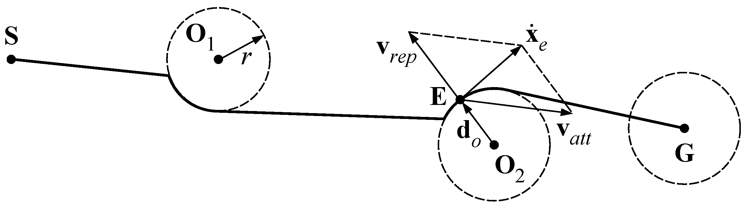
following the minimum potential path towards the goal. As shown in
Figure 1,
is the initial position of the end-effector,
is the goal and
are the obstacles, with their region of influence outlined by their radius
. Moreover:
and
. Based on [
28], Equation (
1) defines attractive and repulsive velocities as:
where the symbol
∇ indicates the gradient operator. Norms of velocities must be set based on the type of application; as an example, values used in the simulations presented in the following of this paper are
and
.
The end-effector trajectory can be found by numerical integration of the resulting velocity:
As a consequence, the end-effector position is iteratively updated by Equation (
2) in accordance with the velocity imposed at each time step. The procedure ends when the distance between the end-effector and the target is lower than a predefined threshold, which is set at
for the examples shown in this paper. Then, an interpolation with a fifth order polynomial law is used to generate a timed motion law over the path previously found. Nevertheless, the trajectory resulting from Equations (
1) and (
2) is typically characterized by short-radius curves and sharp corners that may originate high accelerations and vibration problems, as shown in the example of
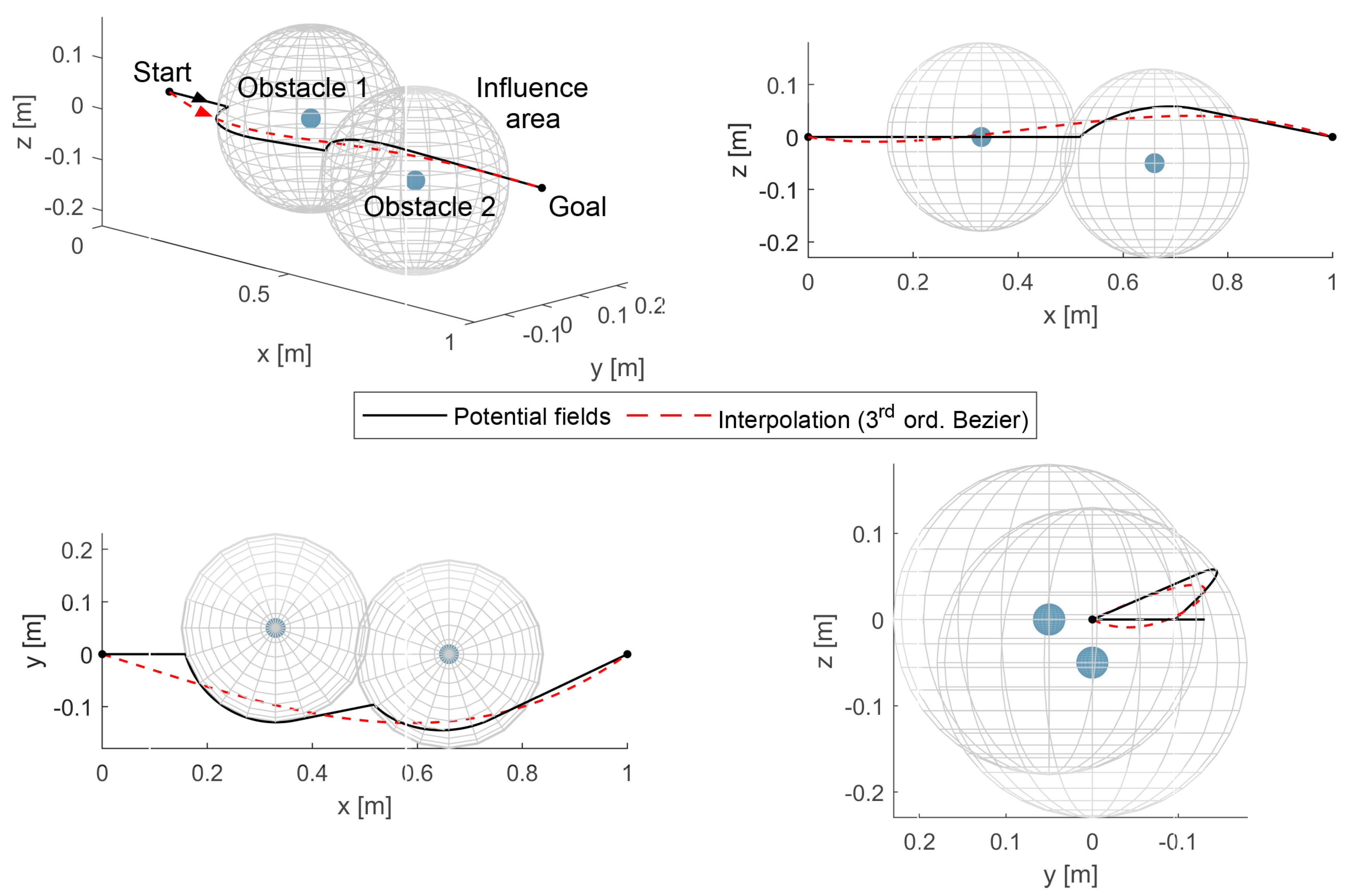
Figure 2: here, two obstacles are interposed between the start and goal points preventing the motion over the ideal linear trajectory; the planning algorithm generates the black curve that remains outside the region of influence of the obstacles in all its points, but presents fast changes of directions in two points, i.e., where the trajectory meets the influence spheres of the obstacles. An interpolation procedure that exploits a smoother type of curve, e.g., a Bézier curve, can be used to solve the problem. In more detail, given
points
, where
n is the power of the Bézier curve, the latter is defined as a parametric function of the variable
s as:
without any loss of generality, let’s consider a third order Bézier curve:
The points
and
being coincident with the starting and goal points, respectively, the fitting procedure seeks for points
and
generating the curve
that best approximates the original one with a least-square metric. Thus, an optimization problem must be solved in order to find the six variables defining points
and
which minimize the quadratic error between the original path and the Bézier curve. A closed-form solution to the problem can be found manipulating Equation (
4) as follows:
If the curvilinear abscissa
s is discretized in
m samples, the trajectory
becomes a set of
m points. Thus, Equation (
6) can be written
m times for the points
, assuming the form:
where:
A closed-form solution for the optimal set of coefficients
can be easily found manipulating Equation (
7) and substituting the matrix
with the analogous matrix
that is built with the points belonging to the trajectory
found with the potential field algorithm:
where † represents the pseudo-inverse operator according to the Moore-Penrose definition, which intrinsically provides the coefficients of the curve that best fits the original trajectory by minimizing the least squares error. An example is given in
Figure 2 in order to show the effect of the smoothing procedure: given the start and goal points and two obstacles preventing from the linear trajectory, the potential fields method described by Equations (
1) and (
2) gives the path plotted in black, whereas the interpolation procedure described by Equations (
3)–(
10) returns the Bézier curve plotted in red. A deeper comparison is given by
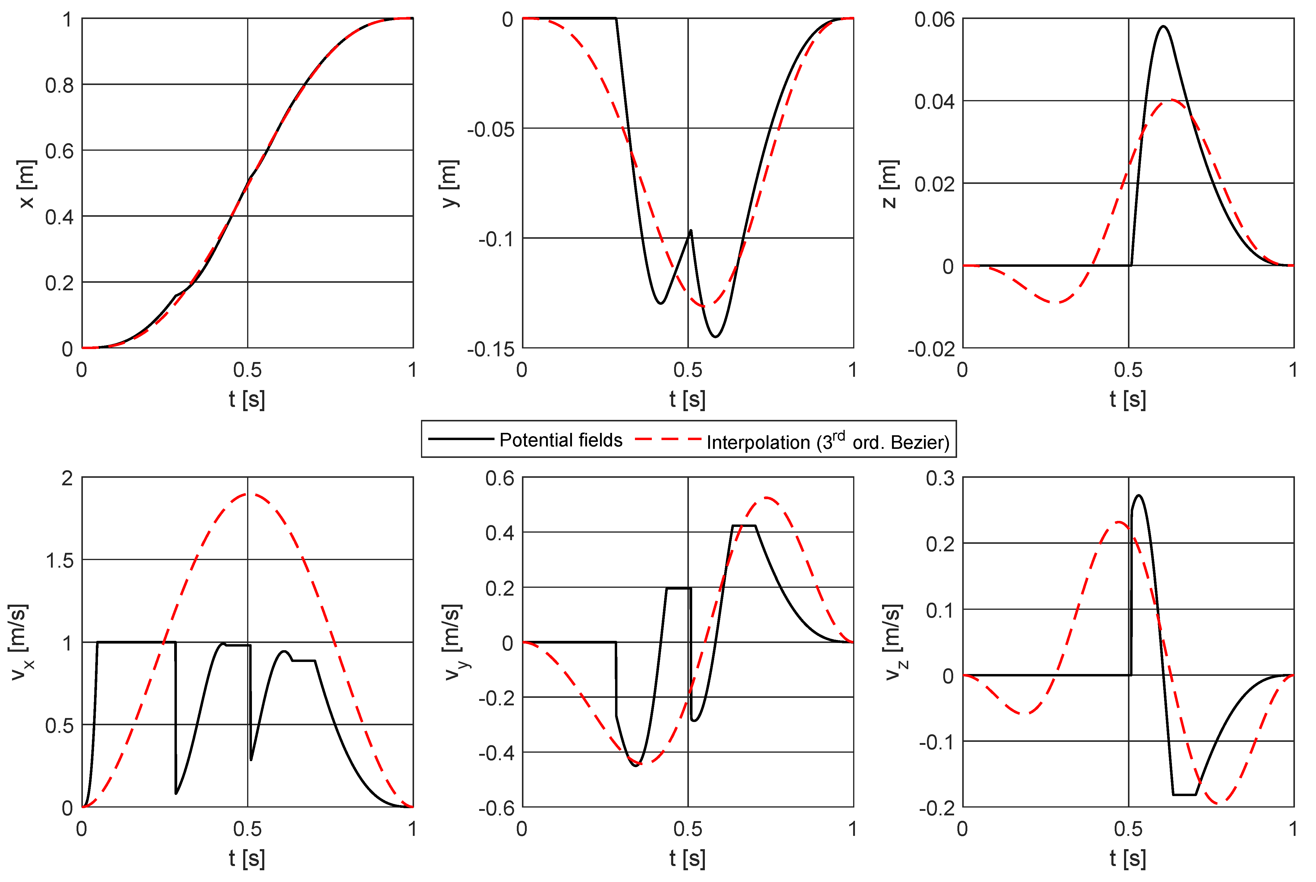
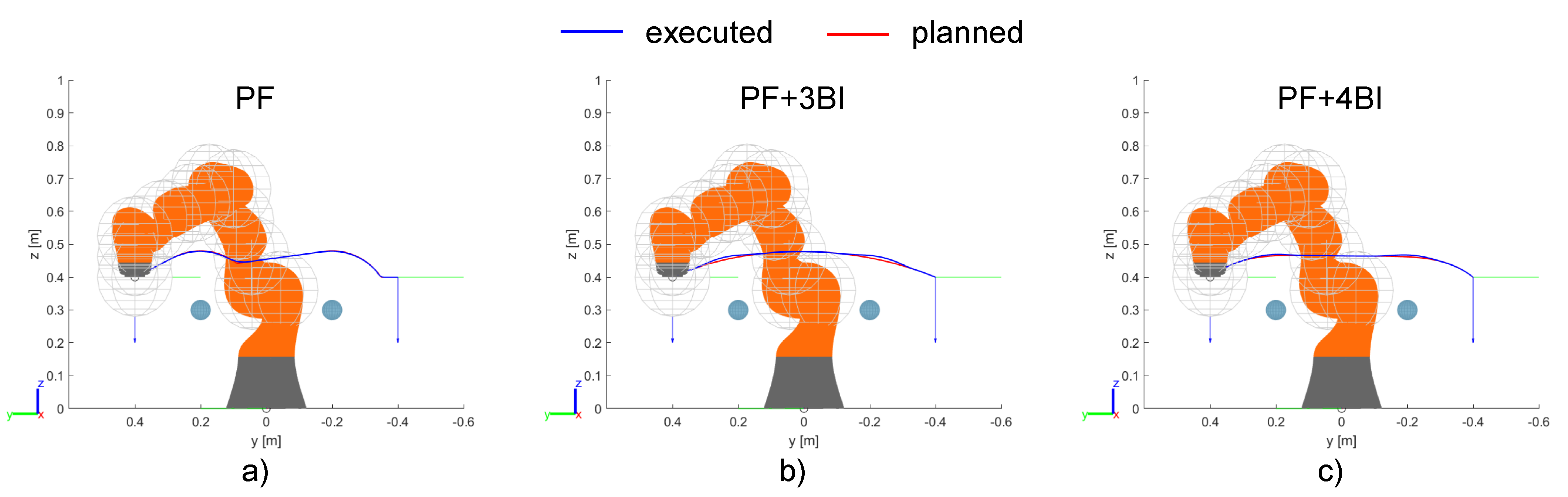
Figure 3, where the Cartesian components of position and velocity of the end-effector are plotted versus time: the path directly obtained by the potential fields algorithm (black plot) presents cusps and discontinuities in the position and velocity profiles, respectively, whereas the trajectory related to the Bézier curve (red plot) is smooth both in position and velocity; thus, it is feasible for it to be assigned to a real manipulator. Bézier curves of higher order have been also tested, but they suffer from too sharp curvatures and high computational times; thus, they are not suitable for the purpose.
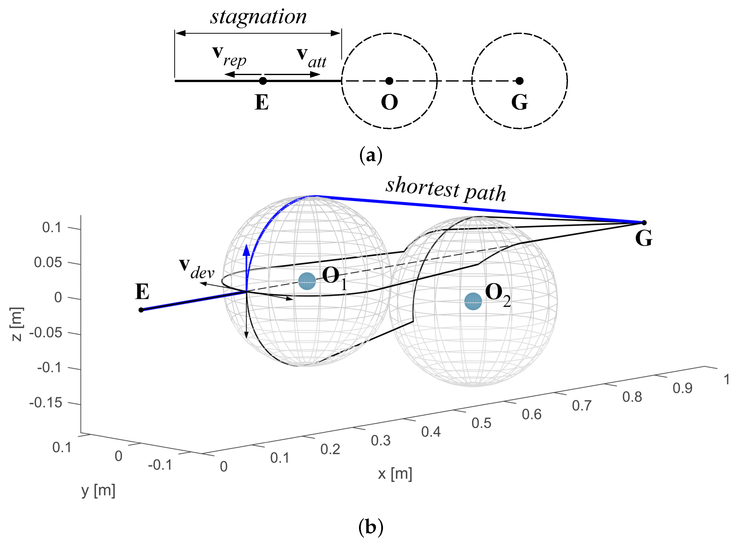
When the potential fields approach is used in path planning a particular condition must be taken into account: as shown in
Figure 4a in a simplified planar scheme, when an obstacle lies exactly on the segment joining the end-effector to the goal point, the attractive and repulsive velocities act in contrast to each other and the end-effector rebounds from the obstacle along such segment, without accomplishing the task. The proposed algorithm overcomes the problem as follows: when the aligning condition between
,
and
is verified, an infinitesimal component of velocity
orthogonal to
is added in order to force the trajectory to exit from the stagnation; among infinite directions that can be assigned to
orthogonal to
, a subset of four of them is selected (aligned with Cartesian axes, with positive or negative directions), whereas its magnitude is constant and predefined. The effect of the deviatoric velocity is to bring the end-effector out of the stagnation line. Obviously, for each one of the selected directions the resulting path is different. Thus, the shortest one is considered for further steps. The example shown in
Figure 4b gives a three-dimensional representation of the problem and shows the trajectories obtained with each one of the four different directions assigned to
; among them the shorted one (blue curve) is chosen.
All the issues discussed above in this section concerned the planning of the Cartesian position of the end-effector of the manipulator, that is, the generation of the motion laws . A different strategy must be defined to generate a smooth transition between the initial and final orientation of the end-effector: if the orientation at the target point is different from the initial one, a linear transition with the same timing law used for the position is defined for the three parameters used for the representation, e.g., the Euler angles.
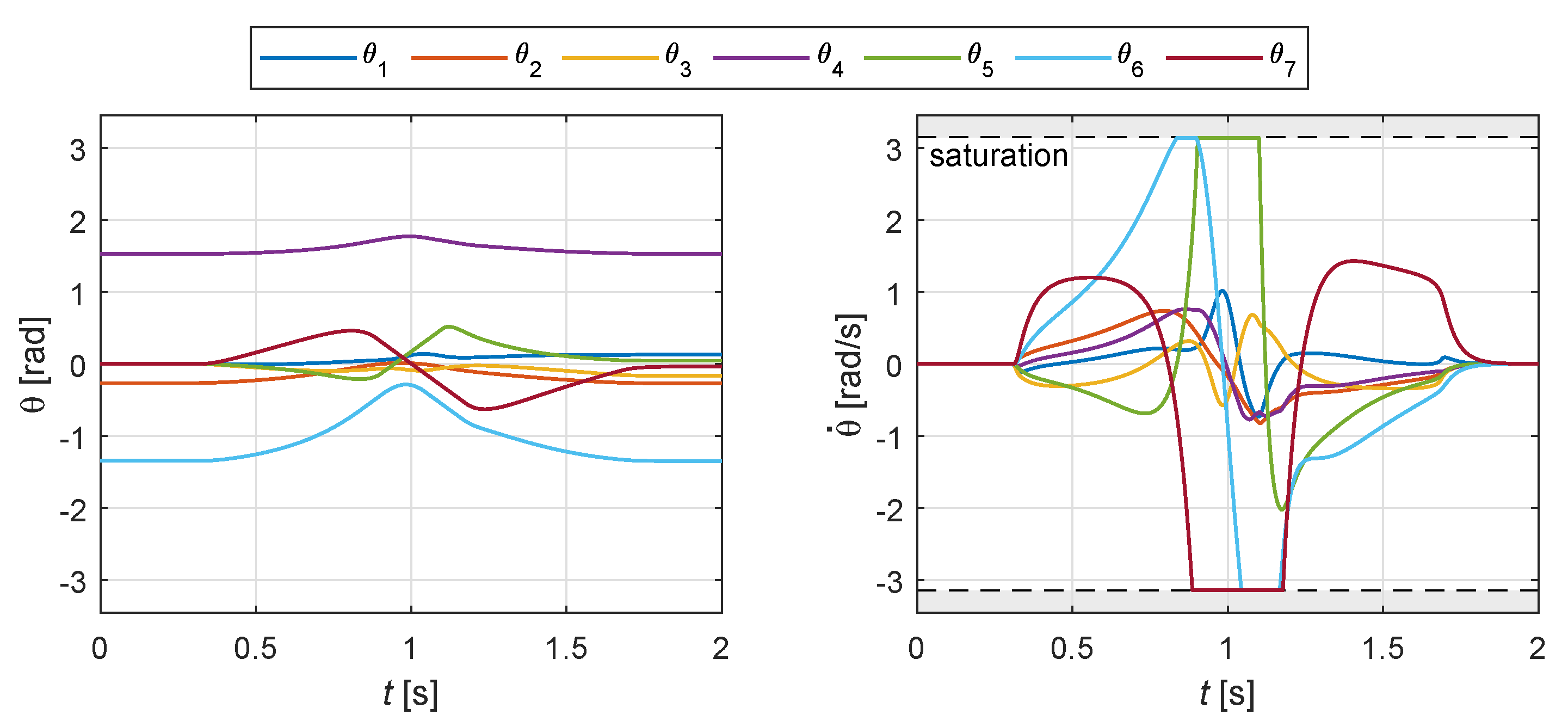
3. On-Line Motion Control
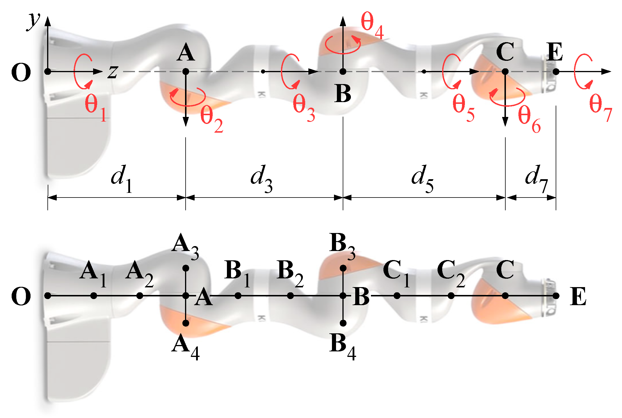
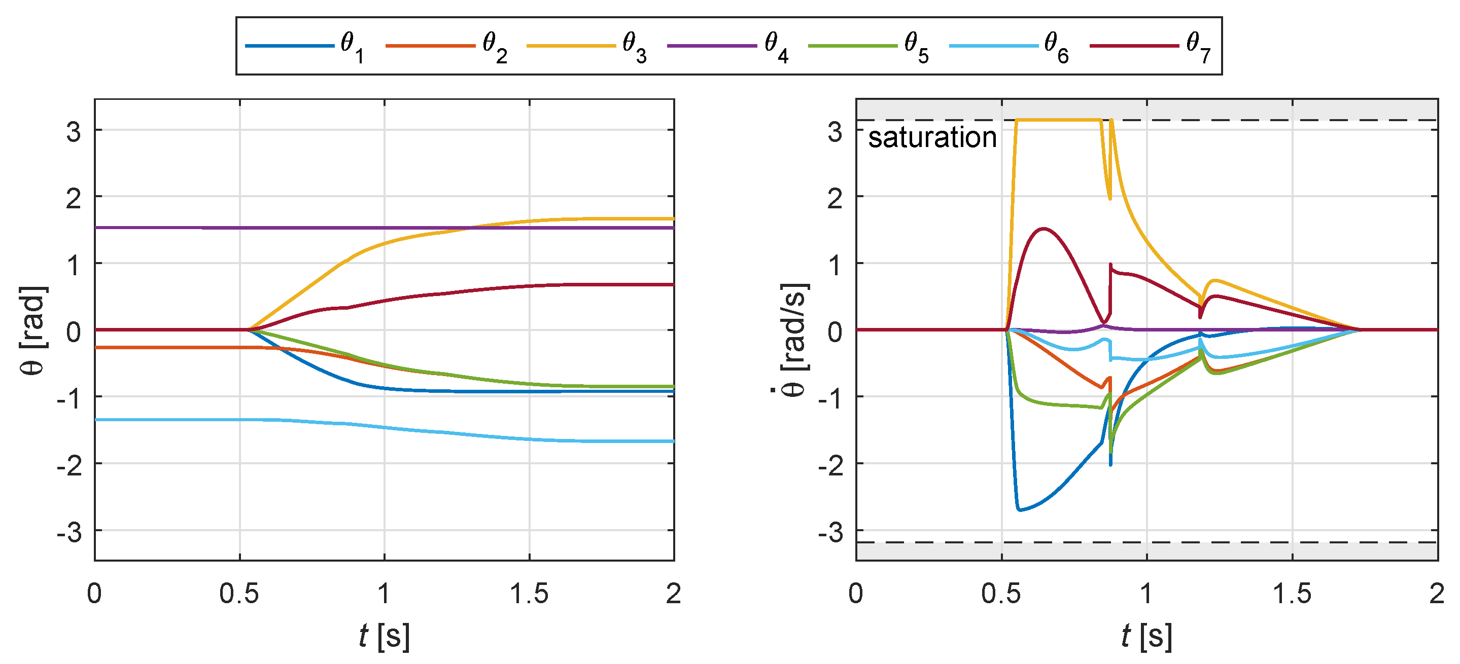
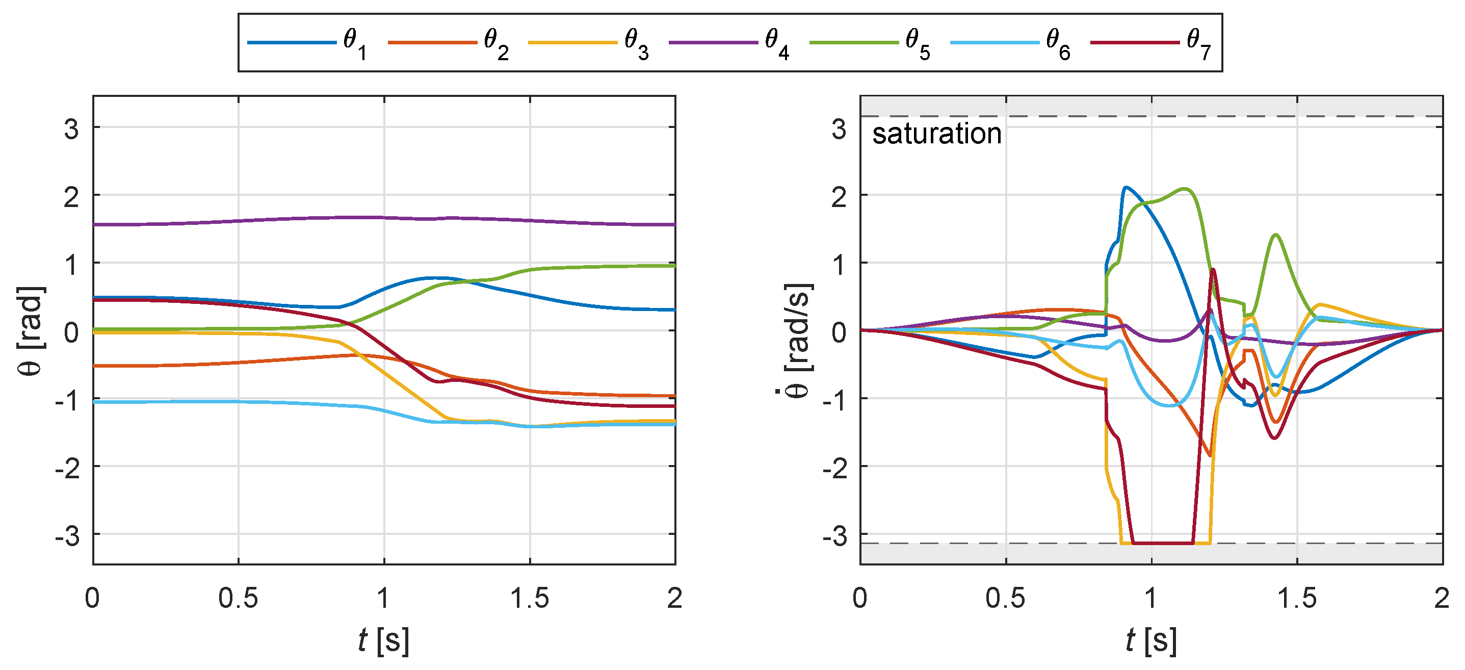
Starting from the results obtained by the authors in [
15], the mentioned algorithms are implemented in the present work for a redundant manipulator with full mobility, i.e., the KUKA LBR iiwa 14 R820 robot. The kinematic scheme of the manipulator is shown in
Figure 5. The pose of the end-effector in the Cartesian space is defined by the vector
, where the last three components are the Euler angles according to the
convention. The seven rotations related to the revolute joints of the serial kinematic chain form the joint space position vector, defined as
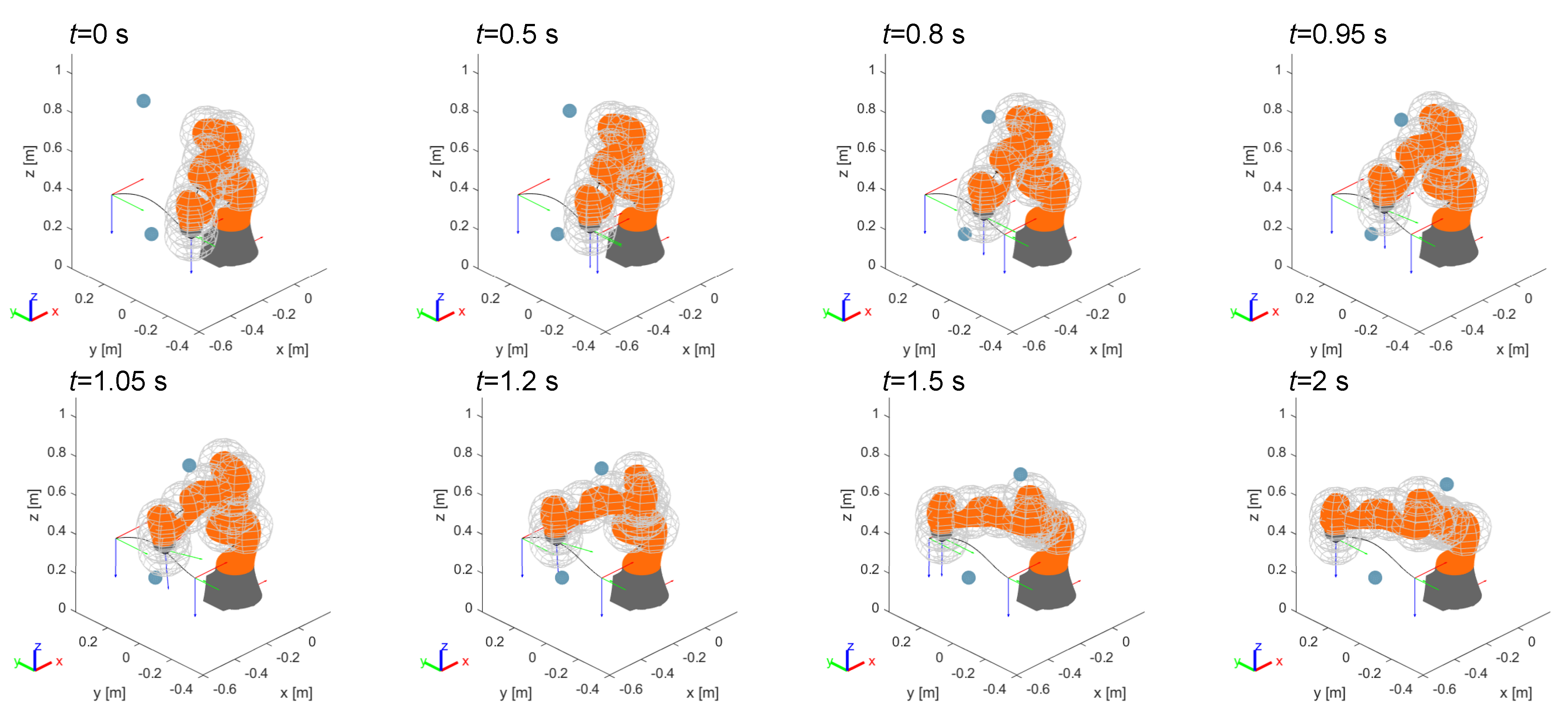
. Thus, the kinematic chain of the manipulator has a redundant degree of freedom with respect to the task. Besides the end-effector
, a total of 13 control points (
) belonging to the kinematic chain characterizes the manipulator, as shown in the bottom picture of
Figure 5.
The forward kinematics of the manipulator can be described by:
In the previous equations
represents the expression of the position forward kinematics and
is the
analytic Jacobian composed by the position and orientation Jacobian matrices
and
, each one of dimensions
; the velocity vector
is composed by the linear velocity
and the angular velocity
, whose expressions, accordingly to the Euler angles
representation, are given by:
Due to redundancy, the inverse position kinematics problem is not uniquely defined, but it can be workedout by the following differential formulation:
The terms of Equation (
14) are defined as follows:
is the joint null space velocity, whose effect is to generate internal motions leaving the pose of end-effector unchanged;
=
is the pseudoinverse of the Jacobian matrix
;
=
is the orthogonal projection into the null space of
.
The inverse kinematic problem formulated in Equation (
14) suffers from numerical problems due to the inversion of the Jacobian matrix when the manipulator is near to a singular configuration, i.e., when the singular values of
tend to zero. In order to avoid singularity problems, the use of the well known damped least-square method was applied [
29]. Such a method consists in the substitution of the pseudoinverse of the Jacobian
by:
where
represents a damping factor that confers a better numerical conditioning to the inversion problem. The value of
should be a compromise between accuracy (low value) and numerical robustness (high value). An efficient way to determine
is to define it as a function of the smallest singular value
of
:
In this way the effect of the approximation vanishes when the smallest singular valuer is greater than a threshold
, where
when
, being
and
tunable parameters of the algorithm. This kind of approximation introduces a position error that must be subsequently recovered by a proportional term in the control law, as typically done in Closed-Loop Inverse Kinematics (CLIK) control laws [
30].
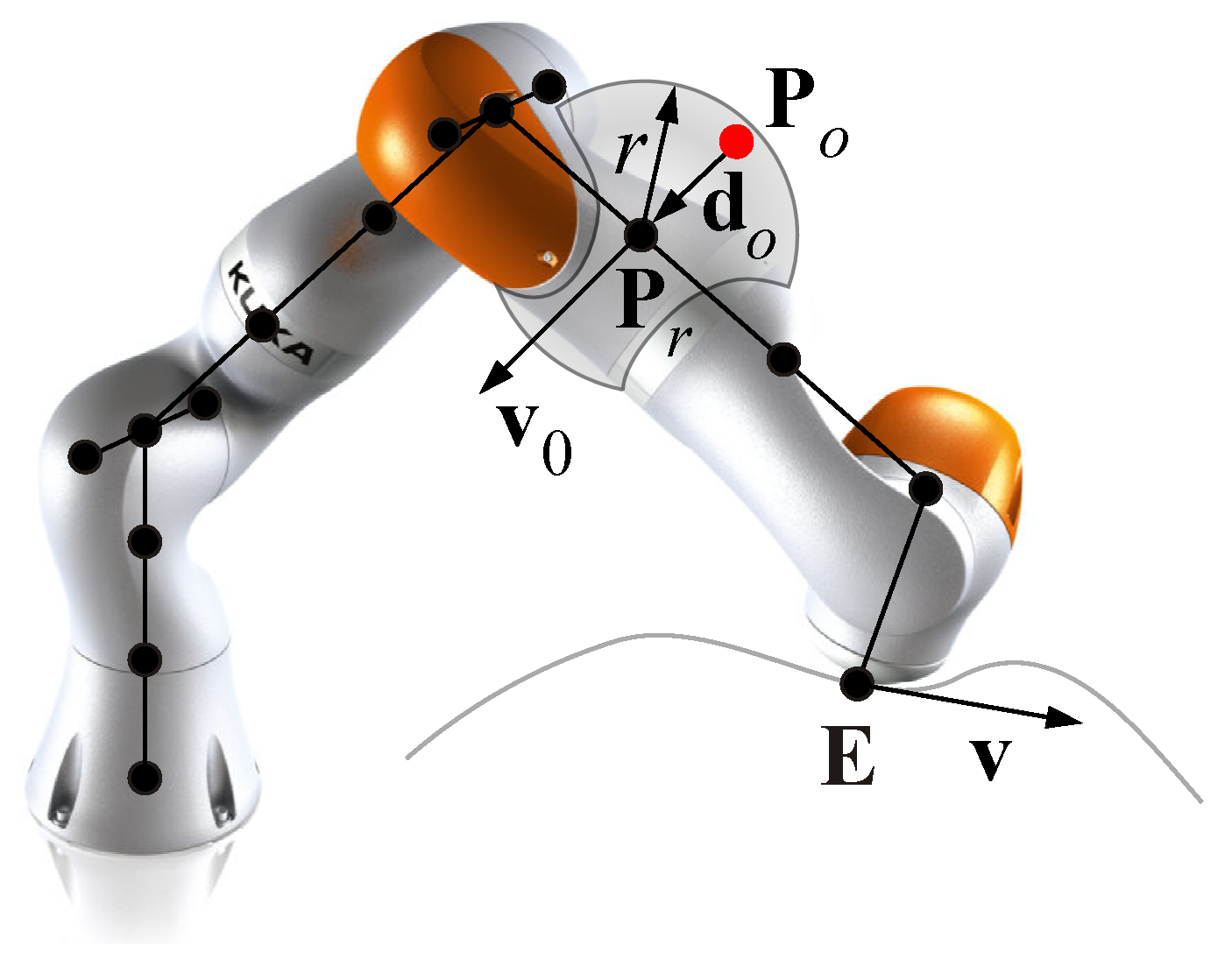
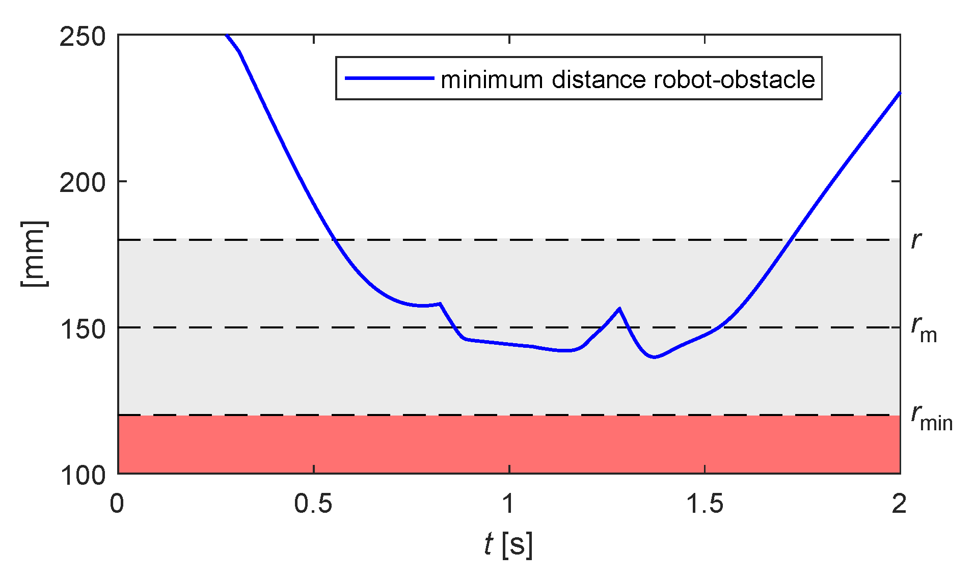
In addition to the basic control law, an obstacle avoidance strategy is introduced: inspired by the null space methods for the control of redundant manipulators [
21], an additional velocity vector is assigned to the control point of the robot which is the closest to one of the obstacles within the workspace, so that the control point can move away form the obstacle, while the motion of the end-effector is not affected. In more detail, referring to the
Figure 6, the couple of points
and
at the minimum distance
is identified at each time step. The region of influence of each control point is delimited by the radius
r. If at a certain time step during the motion the condition
is verified, a repulsive velocity
is imposed to the relative control point along the direction of
. Being the manipulator characterized by one redundant DOF, only one repulsive velocity vector can be assigned at each time step, thus the point to which it is assigned may change over time with the criterion of minimum distance from one of the obstacles. Such a point can be also the end-effector: besides the velocity vector
assigned by the off-line path planning in order to describe the desired trajectory, the repulsive velocity vector can be applied to
, modifying its trajectory, if the position of an obstacle changes from its initial state or a new obstacle enters the workspace, interfering with the motion of
. In this case, the position of the end-effector drifts from the originally planned trajectory, originating a position error analogous to the one related to the damped least-square approximation for the inversion of the Jacobian matrix. Nevertheless, the CLIK control law can be exploited to recover the error.
In terms of equations, the following expressions (
18) and (
19) must be imposed in order to assign the two velocity tasks above described:
where
represents the
upper part of the Jacobian matrix
associated to the velocity of the point
.
Thus, Equation (
14) can be modified in [
31,
32]:
where
,
is the corrected end-effector velocity,
a positive-defined gain matrix (for simplicity defined as
) and
is the position error between the desired position
and the actual position
. The error
can be represented by [
29]:
where the translation error is given by the
vector
and the orientation error is given by the
vector
. The end-effector position is expressed by the
position vector
, whereas its orientation by the
rotation matrix
, with
being the unit vectors of the end-effector frame.
The first term of Equation (
20) guarantees the exact velocity of the end effector with minimum joints speed. The second term drives the motion of the point
of the robot, satisfying the collision avoidance additional task. The choice of
is a critical point of the algorithm. The proposed strategy is to change
according to the distance from the obstacle. To avoid a discontinuity and give smoothness to the motion, two weighting coefficients,
and
, are introduced:
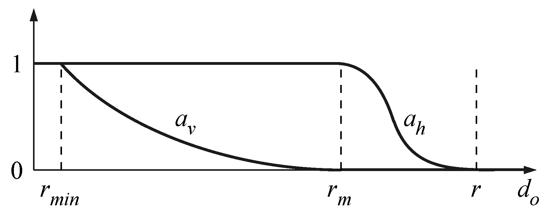
Thus, a nominal repulsive velocity is modulated by as a function of the distance , whereas acts with a weight that balances the effect of the homogeneous solution (related to the collision avoidance) with respect to the total.
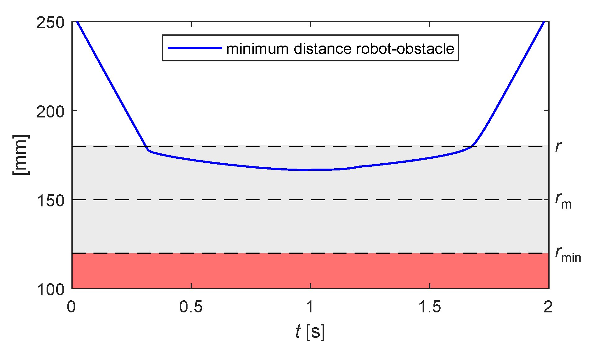
In more detail, let
r be the control distance that defines the region of influence of a control point,
the distance under which no action is possible, and
an intermediate critical distance between
and
r. No influence of the obstacle is desired if
, whereas the algorithm fails (the robot stops) if
. Between these limits the weighting coefficients vary continuously from 0 to 1, as shown in
Figure 7, accordingly to the following expressions [
4]:
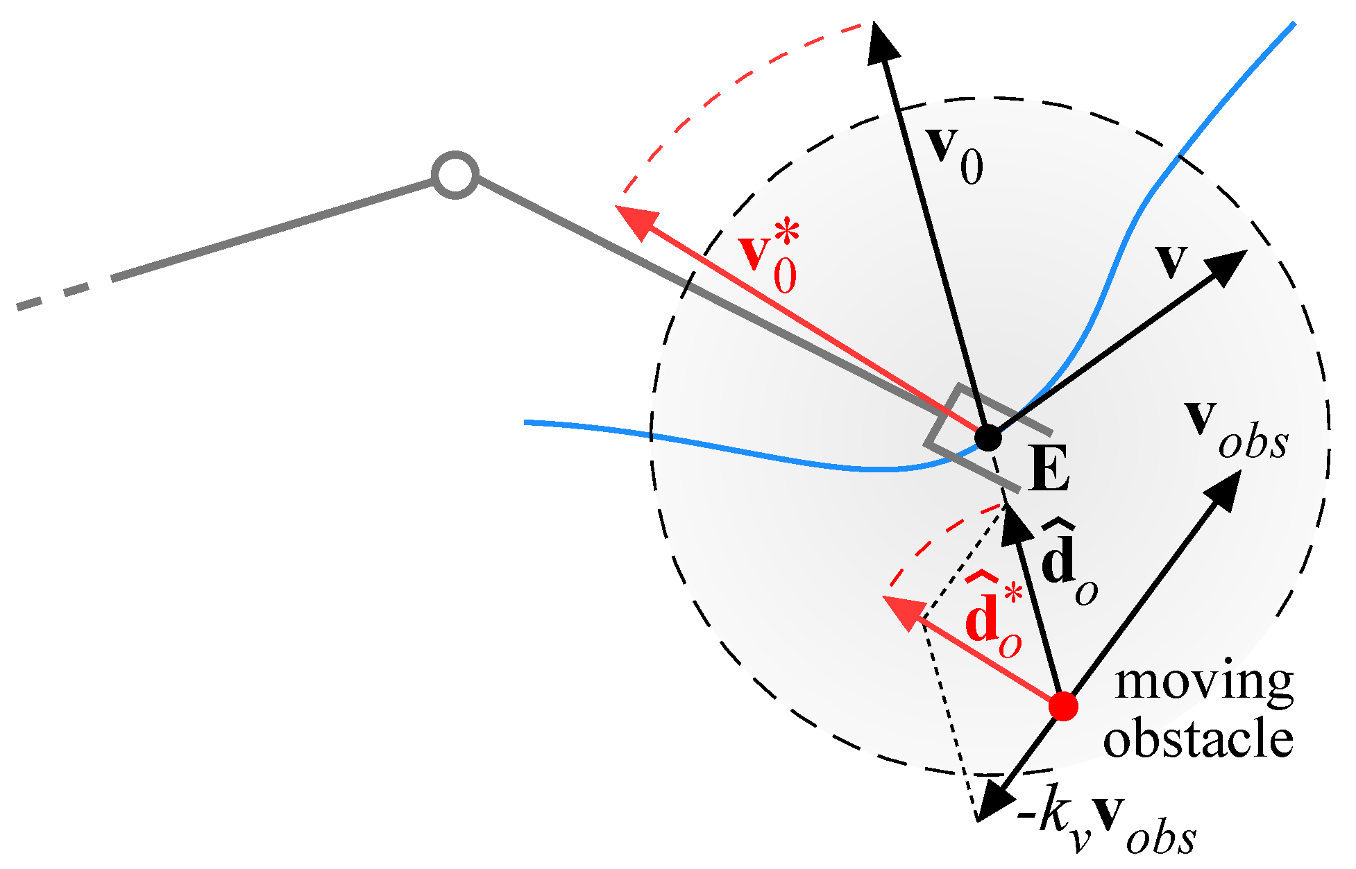
In order to improve the ability of the algorithm to avoid moving obstacles, a modification of the control law expressed by Equation (
23) can be introduced changing the definition of the repulsive velocity [
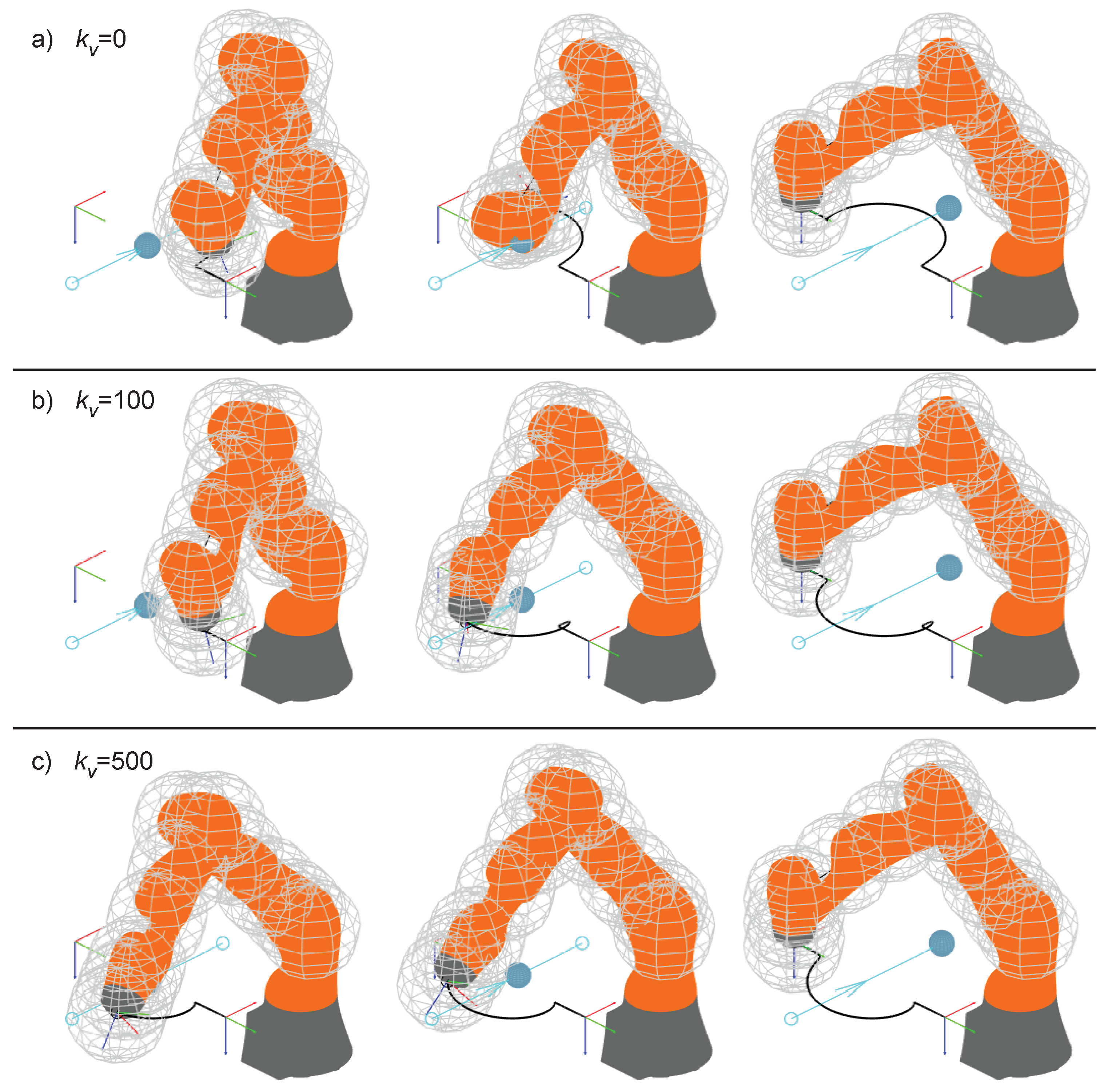
15]: it is reasonable that not only the position, but also the velocity of an obstacle should influence the control of the robot. As an example, if the end-effector moves toward an obstacle having an orthogonal velocity, it is preferable to modify the trajectory of the end-effector pushing it in the direction opposite to the obstacle velocity. Thus, if the end-effector is the control point closest to the obstacle, the repulsive velocity vector
is modified as follows:
where, as described in
Figure 8,
is the obstacle velocity,
is the repulsive velocity along the direction of
,
is a gain term and
is the modified repulsive velocity applied to the end-effector in combination with the planned velocity
. As a consequence, the direction of the repulsive velocity is modified, whereas its magnitude does not change; furthermore, for
, the effect vanishes.


