
Detachment Detection in Cam Follower System Due to Nonlinear Dynamics Phenomenon

Department of Mechanical Engineering, San Diego State University, 5500 Campanile Drive, San Diego, CA 92182-1323, USA
Machines 2021, 9(12), 349; https://doi.org/10.3390/machines9120349
Submission received: 15 September 2021
/
Revised: 18 October 2021
/
Accepted: 21 October 2021
/
Published: 9 December 2021
(This article belongs to the Special Issue Dynamic Analysis of Multibody Mechanical Systems)
Abstract
:The detachment between the cam and the follower was investigated for different cam speeds (N) and different internal distance of the follower guide from inside (I.D.). The detachment between the cam and the follower were detected using largest Lyapunov exponent parameter, power density function of Fast Fourier Transform (FFT), and Poincare’ maps due to the nonlinear dynamics phenomenon of the follower. The follower displacement and the contact force between the cam and the follower were used in the detection of the detachment heights. Multi-degrees of freedom (spring-damper-mass) systems at the very end of the follower were used to improve the dynamic performance and to reduce the detachment between the cam and the follower. Nonlinear response of the follower displacement was calculated at different cam speeds, different coefficient of restitution, different contact conditions, and different internal distance of the follower guide from inside. SolidWorks program was used in the numerical solution while high speed camera at the foreground of the OPTOTRAK 30/20 equipment was used to catch the follower position. The friction and impact were considered between the cam and the follower and between the follower and its guide. The peak of nonlinear response of the follower displacement was reduced to (15%, 32%, 45%, and 62%) after using multiple degrees of freedom systems.
1. Introduction
Follower displacement and the contact force are criteria to the detachment and separation between the cam and the follower at high speeds based on the nonlinear dynamic analysis conception. Largest Lyapunov exponent parameter using average logarithmic divergence, power density function using Fast Fourier transform, and Poincare’ maps are investigated to detect the detachment in nonlinear dynamic phenomenon. The application of this cam–follower system can be found in internal combustion engines.
Sundar et al. used the Hertzian contact theory to calculate the contact stiffness by analyzing the coefficient of restitution model using single degree of freedom when the cam was spinning about a fixed point, [1]. Yan and Tsay solved the separation phenomenon problem between the cam and the follower by increasing the preload rate of the spring force. They proposed a mathematical model for the cam profile with a variable speed to change the follower motion by using Bezier function, [2]. Jamali et al. discussed the parameters that affect the contact problem between the cam and flat-faced follower such as radius of curvature, surface velocities and applied load under thin film of lubricants. They improve numerically the level of film thickness lubricant by taking into consideration the parabolic shape of the pressure distribution through cam depth which reduced the detachment between the cam and the follower, [3]. Pugliese et al. designed an apparatus to measure the contact force using an optical interferometry sensor with high speed camera. They showed different conditions for the contact at low and high magnification to detect the angular positions of the cam, [4]. Ciulli et al. measured the contact force experimentally during the rotation of a circular eccentric cam and an engine spline cam at different rotational speeds and preloads in the presence of lubricant film thickness between the cam and the follower, [5]. Alzate et al. observed experimentally the detachment when the contact force exceeds the restoring force at critical velocity region. They concluded that the detachment and the separation between the cam and the follower occurs when there will be a difference in angular velocity between the cam and the follower at the contact point. The detachment between the cam and the follower has been detected based on bifurcation diagram and chaos, [6]. Desai and Patel determined the critical angular speed when the follower jumps off the cam. They determined the kinematic parameters of the dynamic force analysis at different motion for the follower such as constant velocity motion, cycloidal motion, parabolic motion and simple harmonic motion, [7]. Yang et al. extended a transient impact hypothesis of the contact model by considering the tangential slip between the cam and the follower. They showed that the cam and the follower kept permanent contact at low speeds, while the separation and oblique impact will happen at high speeds, [8]. Lassaad et al. studied the effect of the error in cam profile on the behavior of nonlinear dynamics of the oscillated roller follower by solving the nonlinear second order differential equations, [9]. DasGupta and Ghosh used a constant pressure angle to assess jamming of the follower in its guide based on the follower–guide friction, [10]. Yousuf and Marghitu studied the influence of flank curvature of the cam profile on the nonlinear dynamic behavior of the roller follower at different cam speeds (N) and different follower guides’ internal dimensions (F.G.I.D.). They concluded that the follower motion is non-periodic when the cross-linking of the phase-plane diagram diverges with no limit of spiral cycles by taking into consideration the impact through impulse and momentum theory, [11]. This study is an extension of previous studies in the field of nonlinear dynamics phenomenon in cam follower system. The detachment between the cam and the follower is investigated based on follower displacement and the contact force at different cam speeds (N) and different internal distance of the follower guide from inside (I.D.). The variation of the contact force against time is used in the Lyapunov exponent parameter code to detect for the detachment between the cam and the follower. A positive value of Lyapunov exponent of the contact force indicates non-periodic motion, while a negative value of the Lyapunov exponent reflects the periodic motion of the contact force. Moreover, non-periodic motion of the contact force indicates that there will be a detachment or separation while the periodic motion of the contact force interprets that the cam and the follower stays in permanent contact.
The main contribution of this work is to detect that either the follower will stay in permanent contact with the cam profile or there will be a separation between the cam and the follower.
The manuscript is organized as follows:
(a) In Section 2, the experiment setup was carried out through high speed camera at the foreground of OPTOTRAK 30/20 equipment to catch the follower position and to calculate the contact force. (b) In Section 3, the analytic displacement of the follower was derived using Newton’s second law of translation and rotation motions in the presence of three degrees of freedom for the follower. (c) In Section 4, the detachment between the cam and the follower was detected numerically through follower displacement and contact force using SolidWorks program. (d) In Section 5, Section 6 and Section 7, the detachment between the cam and the follower was detected using largest Lyapunov exponent parameter, power density function of (FFT), and Poincare’ map, respectively.
2. Experiment Test
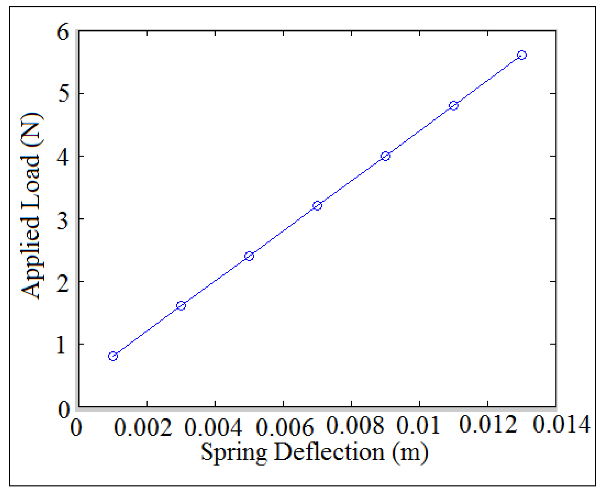
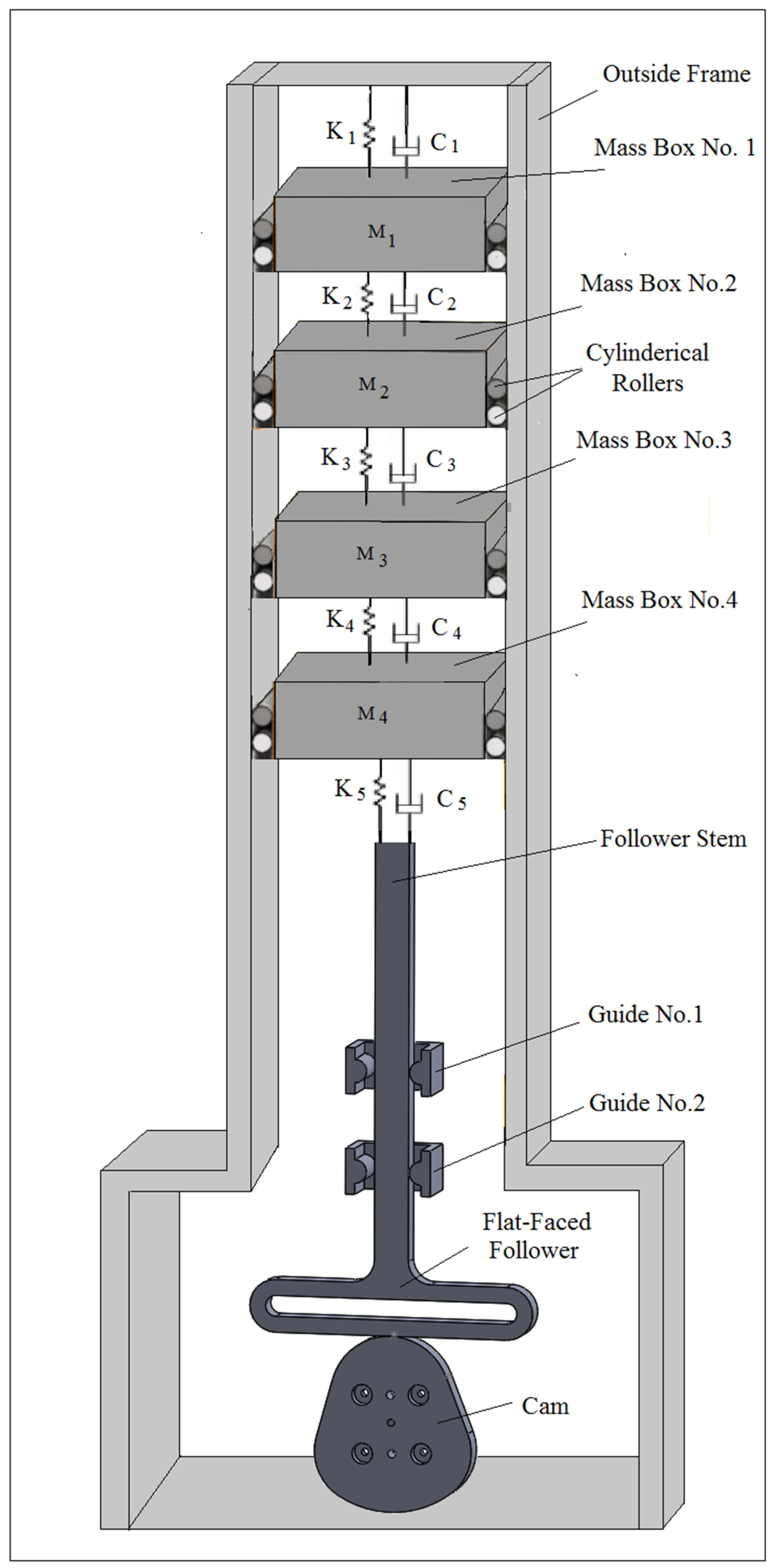
An internal distance of the follower guide (I.D. = 16 mm) with different cam speeds was used in the experiment test. The internal dimension of the follower guide refers to the size of the follower guide from the inside, meaning the distance between the two halves of the cylindrical shape of the follower guide. There was a link between the two halves of the cylindrical shape. The internal distance of the follower guide from the inside was measured to be (I.D. = 16 mm) because it is constant from the manufacturer. The experimental setup was carried out through a high speed camera at the foreground of OPTOTRAK 30/20 equipment to catch the follower position and to determine the contact force. Multi-degrees of freedom (spring-damper-mass) system was used at the very end of the follower stem to keep both cam and follower in permanent contact and to reduce the detachment heights of the follower. All the springs have the stiffness (K1= K2 = K3 = K4 = K5 = 73.56 N/mm) while the coefficient of the damping have the values (C1 = C2 = C3 = C4 = C5 = 9.19 N·s/mm). The masses of the four boxes were (M1 = M2 = M3 = M4 = 0.2625 Kg, Mtotal = 1.05 Kg) to reduce the peak of follower displacement of the lift position. The follower moves with three degrees of freedom in which the contact point was considered in the calculation of follower displacement. The signal of follower movement was derived once and twice to determine the follower acceleration. After multiplying the follower acceleration by the follower mass using Newton’s second law of dynamic motion, the contact force can be experimentally determined [12]. Figure 1 shows the experiment test. Due to the interface feedback of an infrared 3-D camera of the OPTOTRAK / 3020 device, the follower movement was stocked in an Excel file. The follower displacement was processed using MatLab software. To retain the contact between the cam and the follower, a spring with the specification [13] such as spring index (C = 3), number of turn (n = 6), modulus of rigidity (G = 80 GPa.), coil diameter (d = 2.5 mm), outside diameter (OD = 10 mm) and preload extension (Δ = 15 mm) had been used between the vertical table and follower stem. The spring was suspended from a fixed point, and the load was applied at the very end point of the spring. The spring deflection was recorded against the applied load, [14] in which the slope represented the spring stiffness (K = 400 N/m) as indicated in Figure 2.
The jumping phenomenon started at critical operating speed (N = 212 rpm) in which the cam lost the contact with the follower. The critical operating speed of the cam was calculated by equating the summation of the weight and the spring force with the inertia force of the follower, [15]. The impact between the cam and the follower was considered based on impulse and momentum theory because the impact velocity was illustrated in the following equation:
where
- Δh is the change in follower displacement when the follower is turned with an angle (θ) about z-axis, mm.
- g is the gravitational acceleration, mm/s2
- is the change in time when the follower displacement has been changed, s.
The following equation was used to calculate the critical speed of the cam if the spring force was constant and equal to the preload.
where
- r is the minimum radius in the cam profile which is equal to (22.5 mm), [16].
- S is the total force acting on the follower in the direction of the axis when the mechanism is stopped in the minimum lift position, N.
- is the weight which locates at the end of the follower stem, kg.
- ω is the critical speed of the cam, rpm.
The total force (S) represents the impulse force as follows:
Substitute Equation (1) into Equation (3) and Equation (3) into Equation (2) to obtain the parameter () and this parameter disappeared from Equation (2):
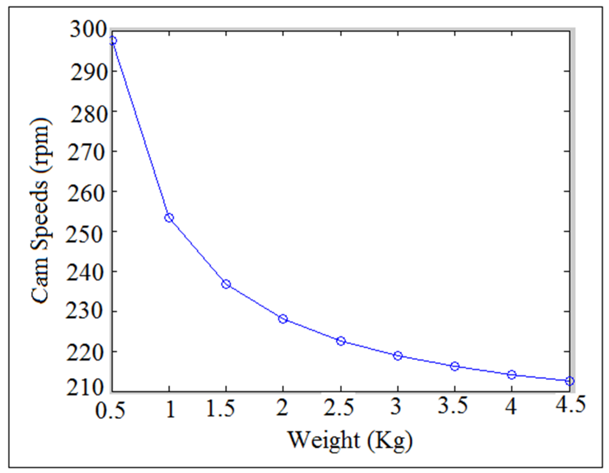
Figure 3 showed how the critical jumping speed of the cam was decreased with the increasing weight where the spring force was constant and equal to the preload until the cam speed settled down. It was hard to operate the cam experimentally over (N = 200 rpm) when the detachment occurred and the cam follower system was collapsed, in which some of the cam profile material took away due to impact, high temperature and friction. For the purpose of comparison with the numerical simulation, both cam and follower were made from plastic material.
3. Equations of Motion of Three Degrees of Freedom System
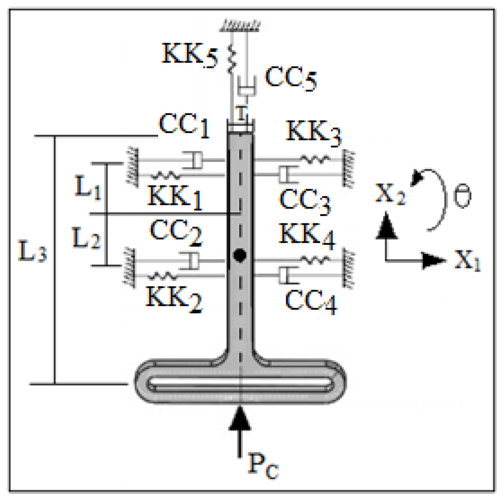
In this paper, the nonlinear dynamics phenomenon occurred due to the motion of the follower with three degrees of freedom (right-left, up-down, and rotation about z-axis). Newton’s second law of the dynamic motion was applied to describe the three degrees of freedom of the follower. Figure 4 showed the mechanical vibration representation of the three degrees of freedom system for the flat-faced follower and its guide. All the springs have the stiffness (KK1 = KK2 = KK3 = KK4 = KK5 = 73.56 N/mm) while the coefficients of the damping have the values (CC1 = CC2 = CC3 = CC4 = CC5 = 9.19 Ns/mm). The mass of the follower was (m = 0.2759 Kg). The cam follower mechanism can be treated as a single or multi-degrees of freedom based on the motion of the follower, [17]. The impedance matrix can be put into terms of frequency response matrix, [18]. The contact force expression in terms of the pressure angle has been taken from, [19,20]. The equations of motion with the solution can be seen in Appendix A.
4. Numerical Simulation
4.1. Detachment Detection through Follower Displacement
- (a)
- SolidWorks program was used in the modeling of computer aided design (CAD), [21]. In the numerical simulation, the follower moved with three degrees of freedom (up-down, right-left, and rotation about z-axes). The two rollers in both sides between the wall and the mass of the spring–damper system helped the multi-degrees of freedom moved up and down as indicated in Figure 5. In SolidWorks program, there were three types of integrator, (GSTIFF), (SI2-GSTIFF) and (WSTIFF), in which the integrator of the type (GSTIFF) was selected. The (GSTIFF) solves the complex nonlinear dynamics system, and it can be operated over a range of speeds of the cam. The integrator (GSTIFF) works with maximum iteration (50), initial integrator step size (0.0001), minimum integrator step size (0.0000001), and maximum integrator step size (0.001). The dimensions of cam, flat-faced follower, and the two guides are taken from Ref. [22] while the dimensions of the outside frame and the four mass boxes are assumed to be arbitrary. The SolidWorks simulation setup can be seen in Appendix B. In regards to the multi-degrees of freedom at the very end of the follower stem, all the springs have the stiffness (K1 = K2 = K3 = K4 = K5 = 73.56 N/mm) while the coefficients of the damping have the values (C1 = C2 = C3 = C4 = C5 = 9.19 Ns/mm). The values of the masses of the four boxes are (M1 = M2 = M3 = M4 = 0.2625 Kg, Mtotal = 1.05 Kg) to reduce the peak of follower displacement of the lift position. The spring constants are the spring index (C = 3), number of turn (n = 6), modulus of rigidity (G = 80 GPa.), coil diameter (d = 2.5 mm), and outside diameter (OD = 10 mm). In regards to the spring between the follower stem and the vertical table, the spring index (C = 3), number of turn (n = 6), modulus of rigidity (G = 80 GPa.), coil diameter (d = 2.5 mm), outside diameter (OD = 10 mm), and the spring stiffness (K = 400 N/m).
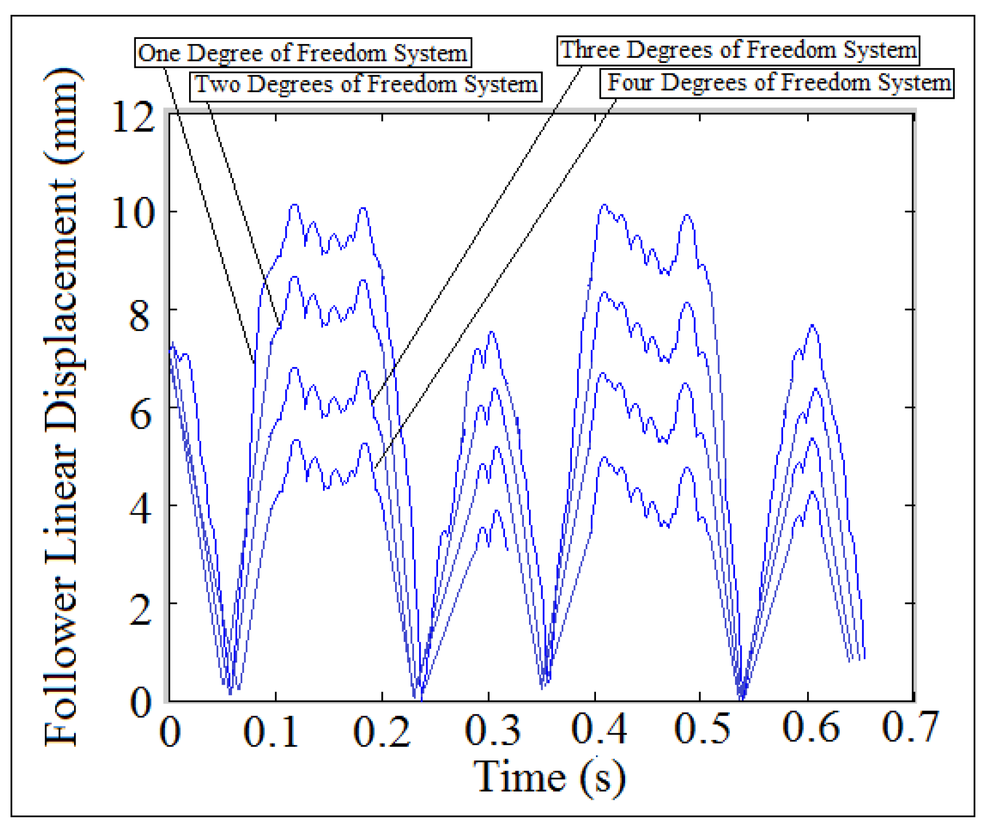
Multi-degrees of freedom was used to reduce the detachment between the cam and the follower and to improve the dynamic performance through the reduction in the peak of the nonlinear response of the follower as shown in Figure 6. The peak of nonlinear response of the follower displacement was reduced to (15%, 32%, 45%, and 62%) after using multi-degrees of freedom systems. Four spring-damper-mass systems are used at the very end of the follower stem to reduce the detachment between the cam and the follower as low as possible and to keep the cam and the follower in permanent contact. The system with internal distance of the follower guide (I.D. = 17 mm) and cam speed (N = 300 rpm) was used in the simulation.
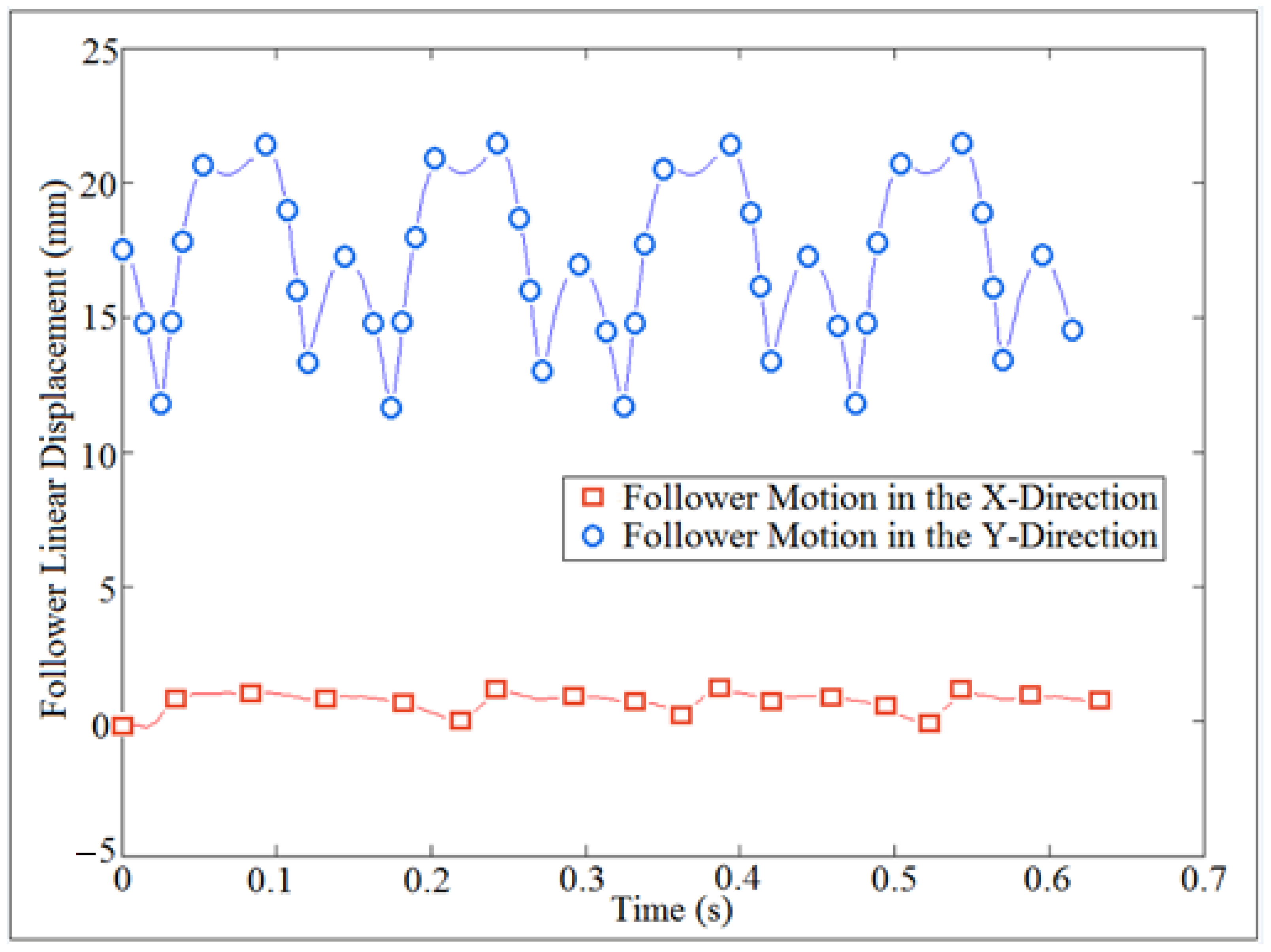
As stated earlier, the follower moved with three degrees of freedom because of the clearance between the follower and its guide. The variation of nonlinear response of the follower displacement was intangible in the x-direction while there was a variation in the y-direction for the follower displacement as indicated in Figure 7.
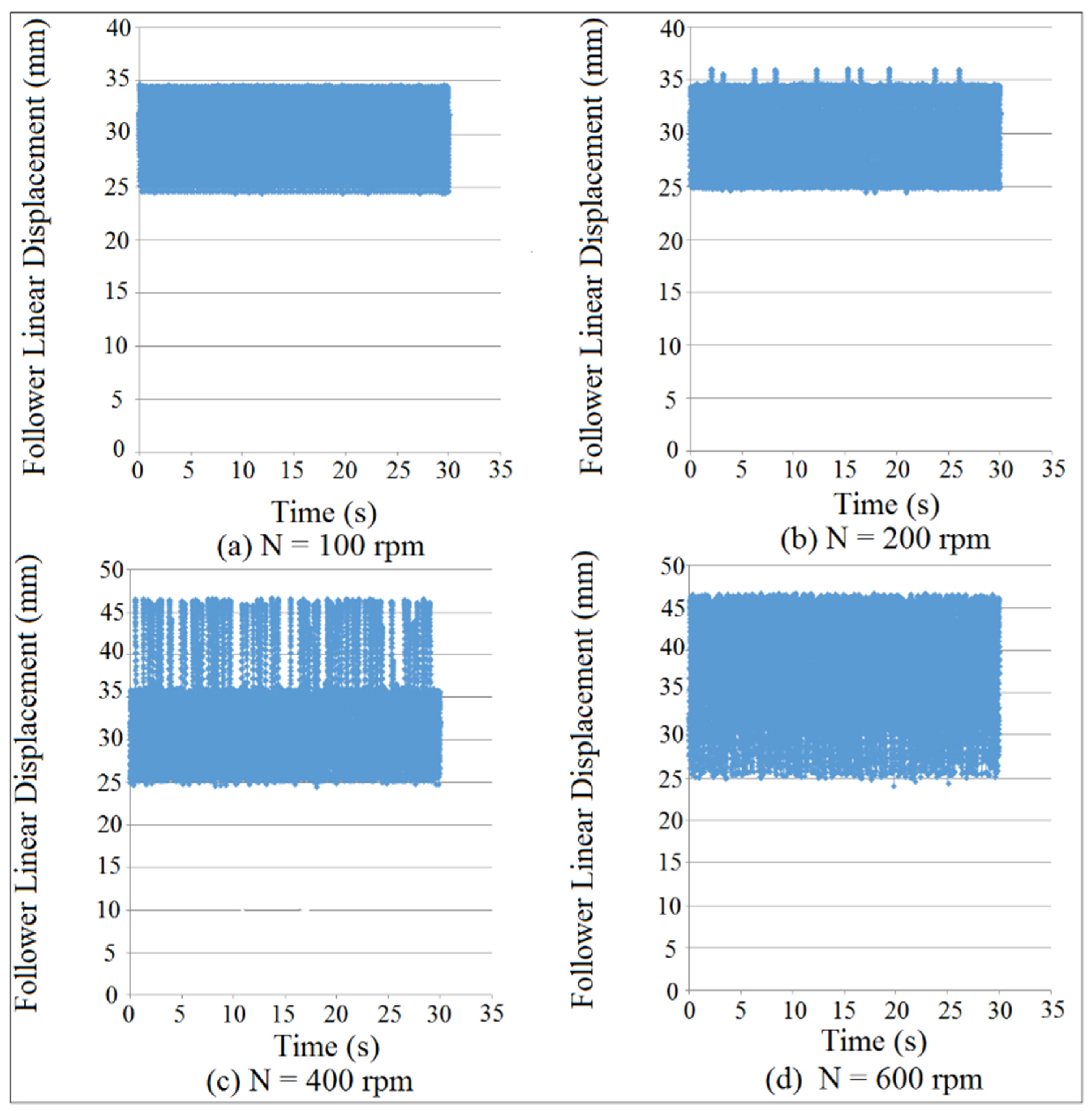
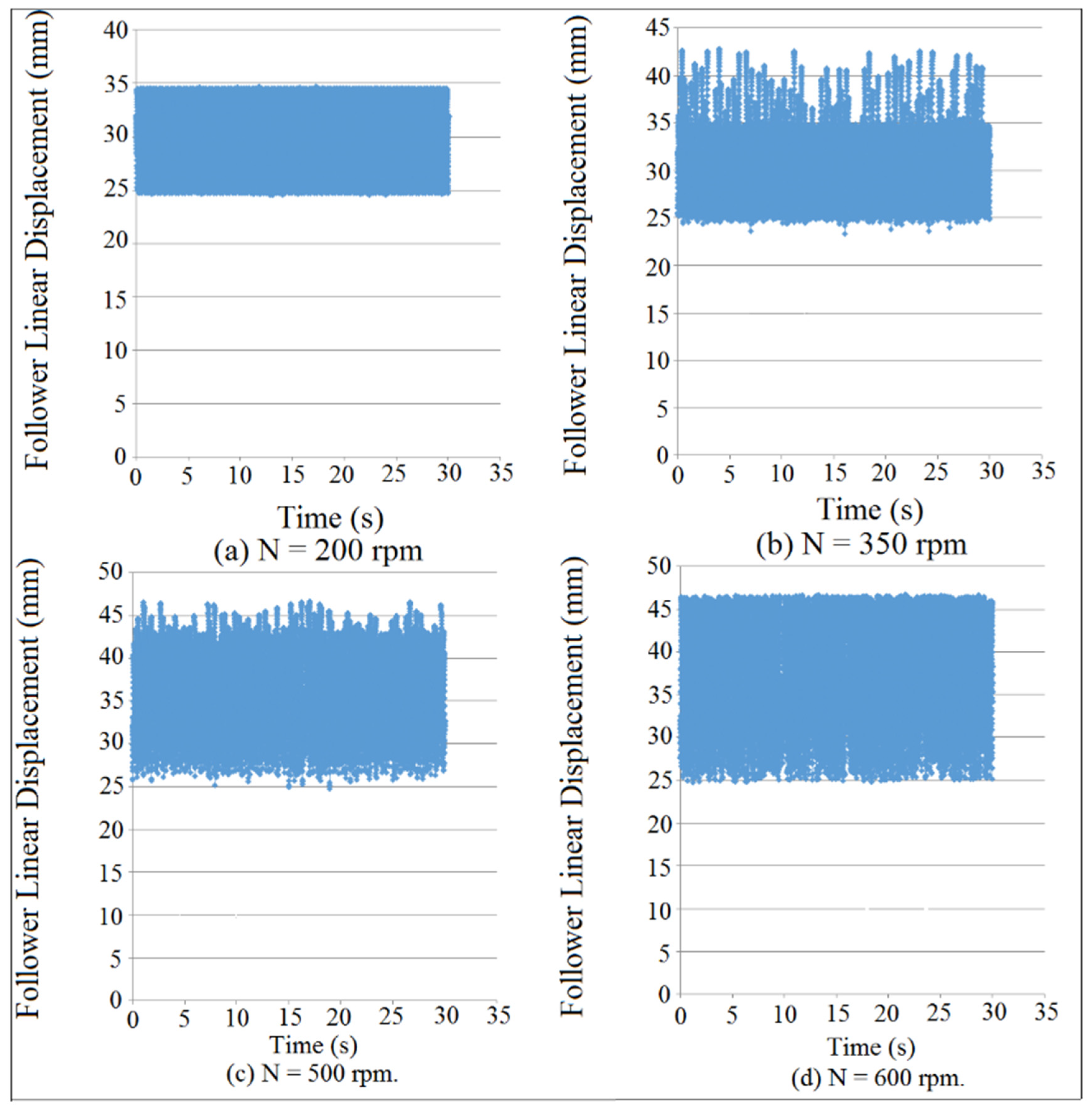
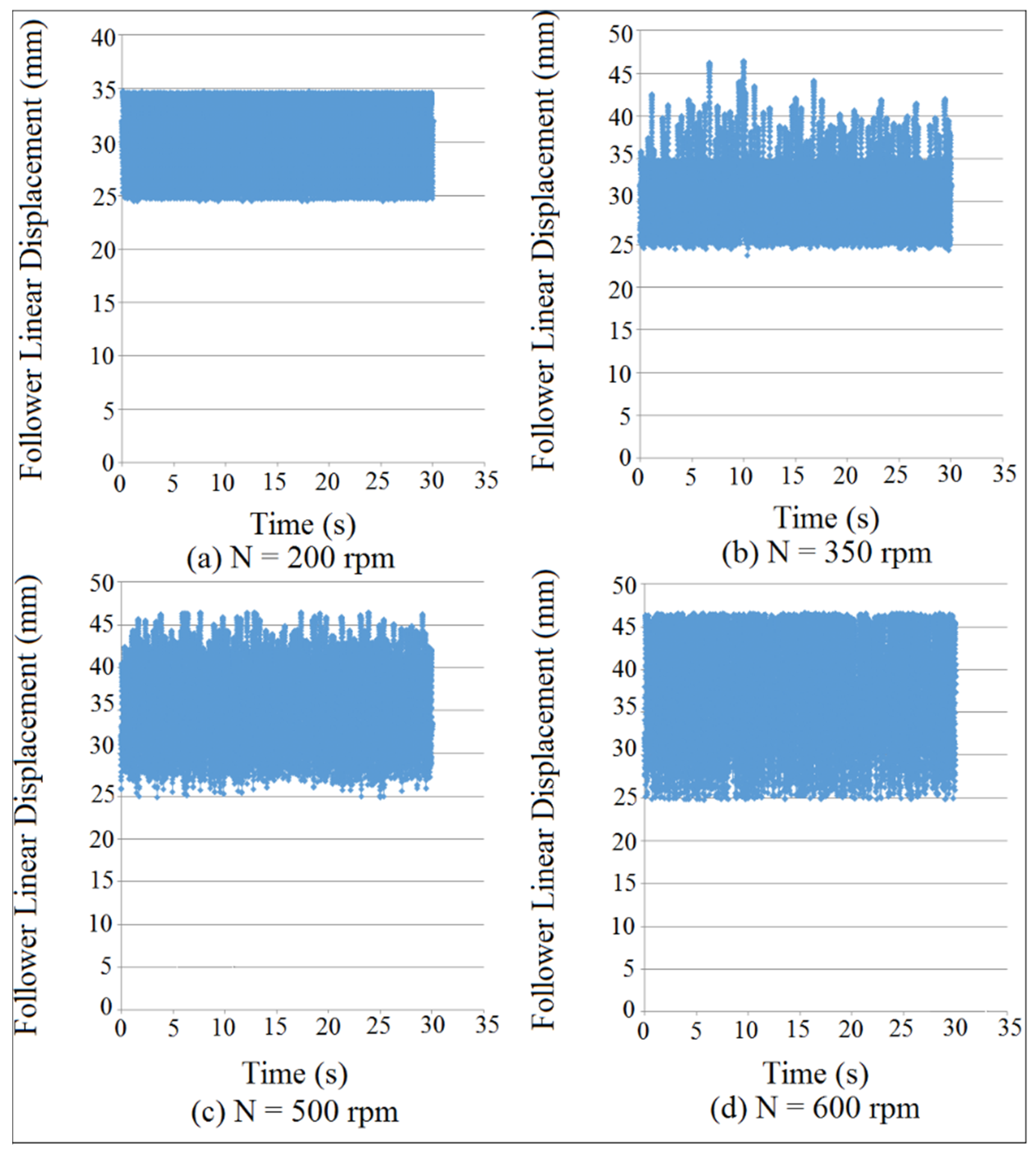
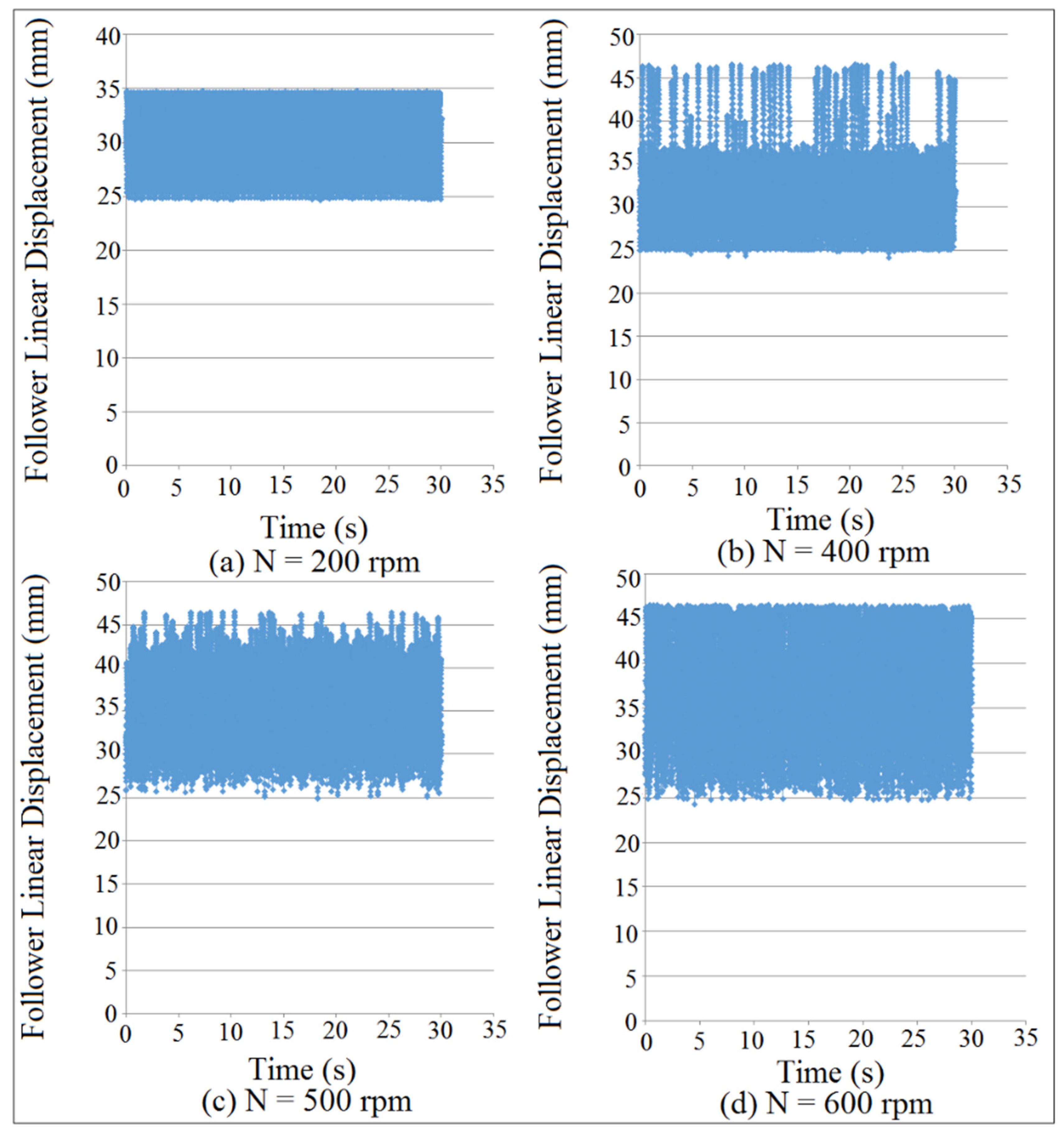
Four different internal distance of the follower guide such as (I.D. = 16, 17, 18, 19 mm) were used in the simulation of the follower displacement and the contact force in which the clearance between the follower and its guide has a variable value. Figure 8 and Figure 9 showed the follower linear displacement mapping against time for (I.D. = 16 and 17 mm), and these figures indicated how the follower detaches from the cam profile at different cam speeds. The follower stayed in permanent contact with the cam profile as shown in Figure 8a and Figure 9a at (I.D. = 16 and 17 mm) and (N = 100 and 200 rpm), respectively. The follower started the detachment from the cam profile as shown in Figure 8b and Figure 9b at (I.D. = 16 and 17 mm) and (N = 200 and 350 rpm), respectively. The follower started multi-detachments and multi-impacts in one cycle of the cam rotation as shown in Figure 8d and Figure 9d at (I.D. = 16 and 17 mm) and (N = 600 rpm). In general, the detachments between the cam and the follower was increased with the increasing of internal distance of the follower guide (I.D.) and cam speeds (N).
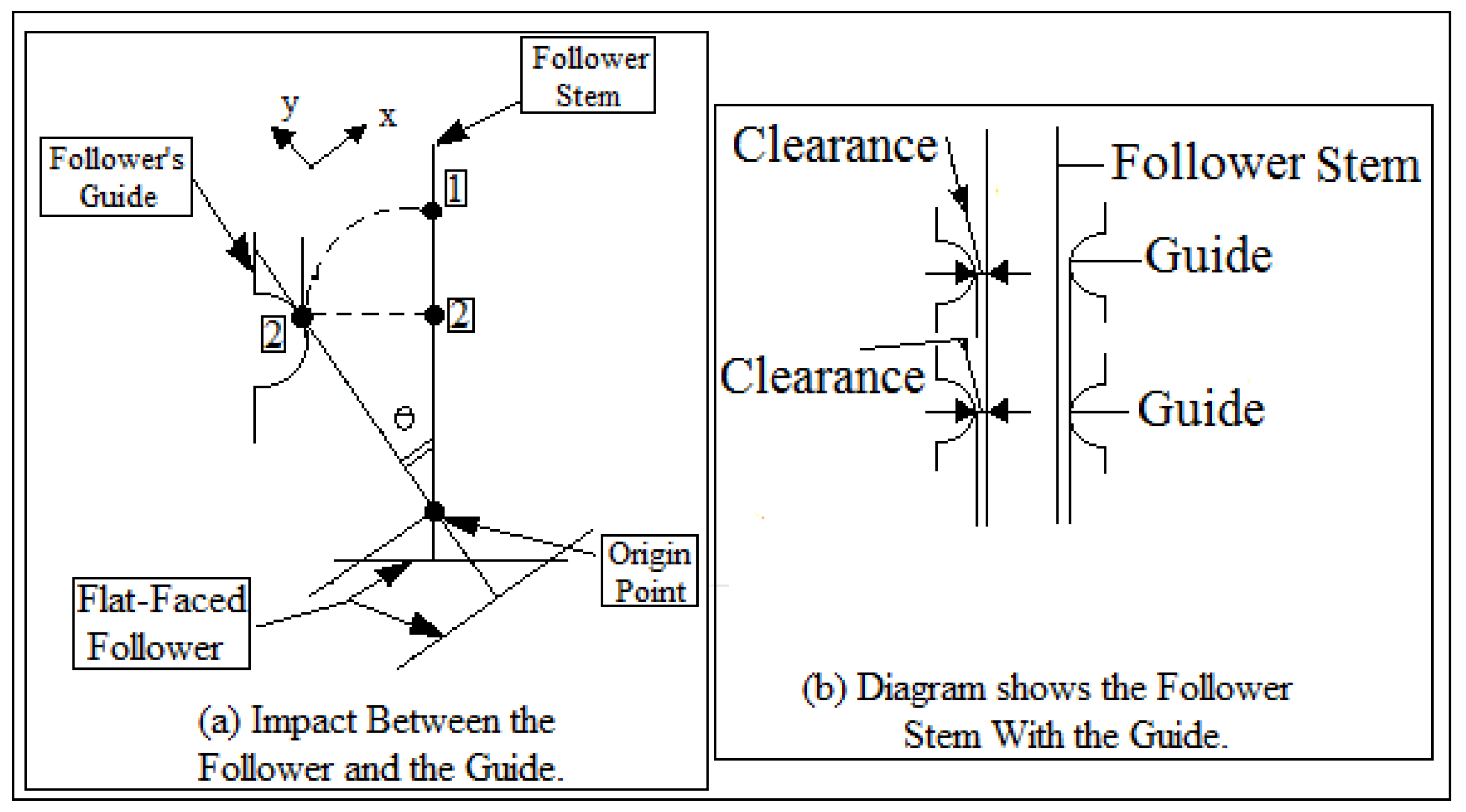
The impact between the follower and its guide was shown in Figure 10a, while the follower stem with its guide was shown in Figure 10b. The impact was analyzed at the contact point based on different values of coefficient of restitution, while the contact was investigated using steel greasy and steel dry frictions. When the value of contact force is a maximum value, it means that the cam and the follower are in permanent contact. On the other hand, when the value of contact force is zero, it means that the follower will detach from the cam at high speeds.
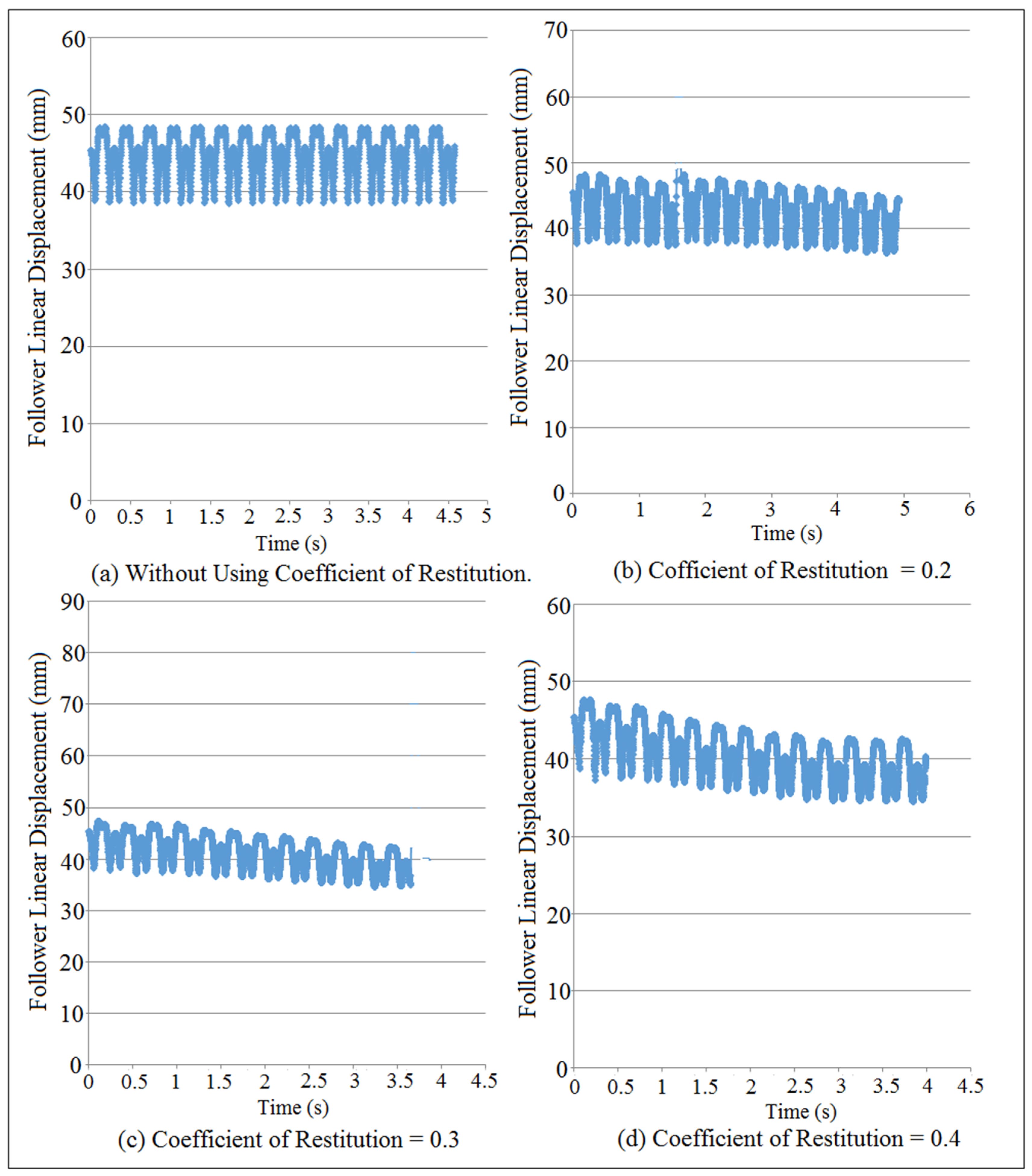
Figure 11 showed the follower displacement mapping against time at different coefficient of restitution values for (I.D. = 19 mm) and (N = 200 rpm). SolidWorks program was used in the simulation of follower displacement. Coefficient of restitution induces impact and is defined as a loss in potential energy due the reduction in the peak of nonlinear response of the follower. There were no losses in potential energy when the cam and the follower were in permanent contact as indicated in Figure 11a. The potential energy losses were increased with the increasing of coefficient of restitution due to the impact until the peak of nonlinear response of the follower displacement settles down as shown in Figure 11b–d. In general, when both the cam and follower are in permanent contact, it means there was no loss in potential energy and there was no either impact or coefficient of restitution. The detachment between the cam and the follower was increased with the increasing of the coefficient of restitution in the presence of the impact.
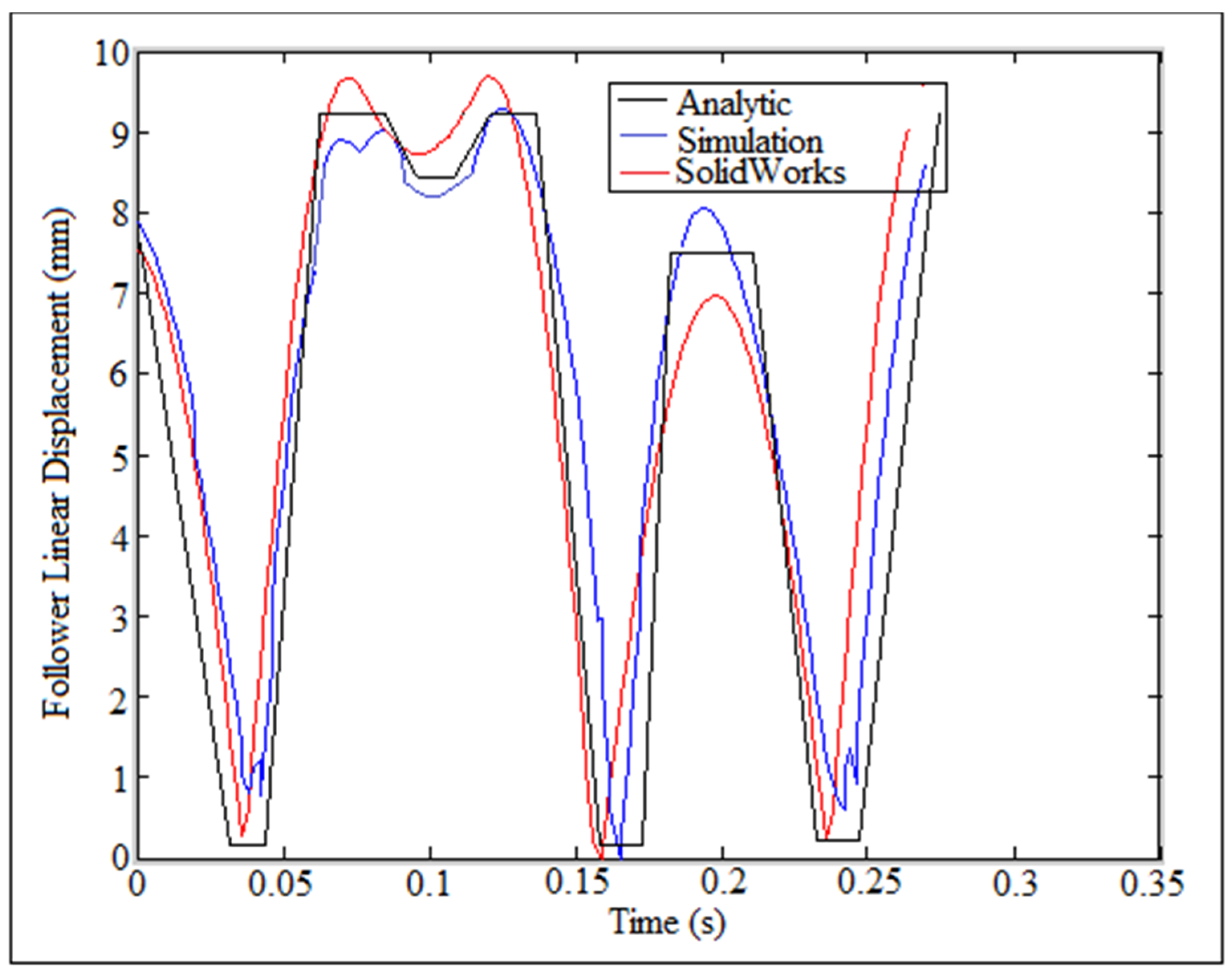
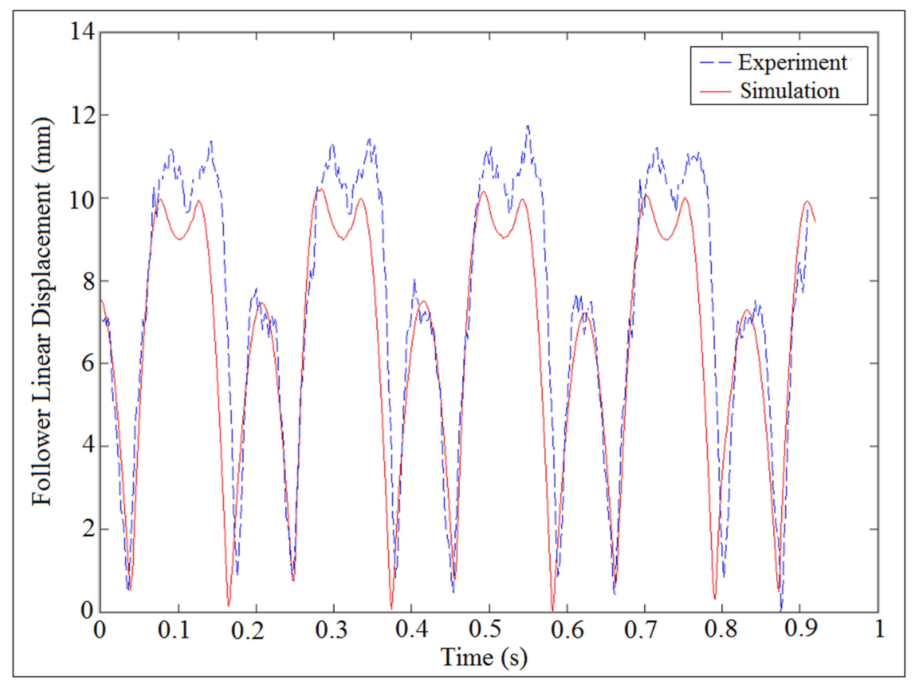
In this paper, the cam profile with return-dwell-rise-dwell-return-dwell-rise-dwell-return-dwell-rise-dwell was selected, [23]. The system with (I.D. = 16 mm) and (N = 200 rpm) was used in the verification of the follower displacement as shown in Figure 12 for one cycle of cam rotation.
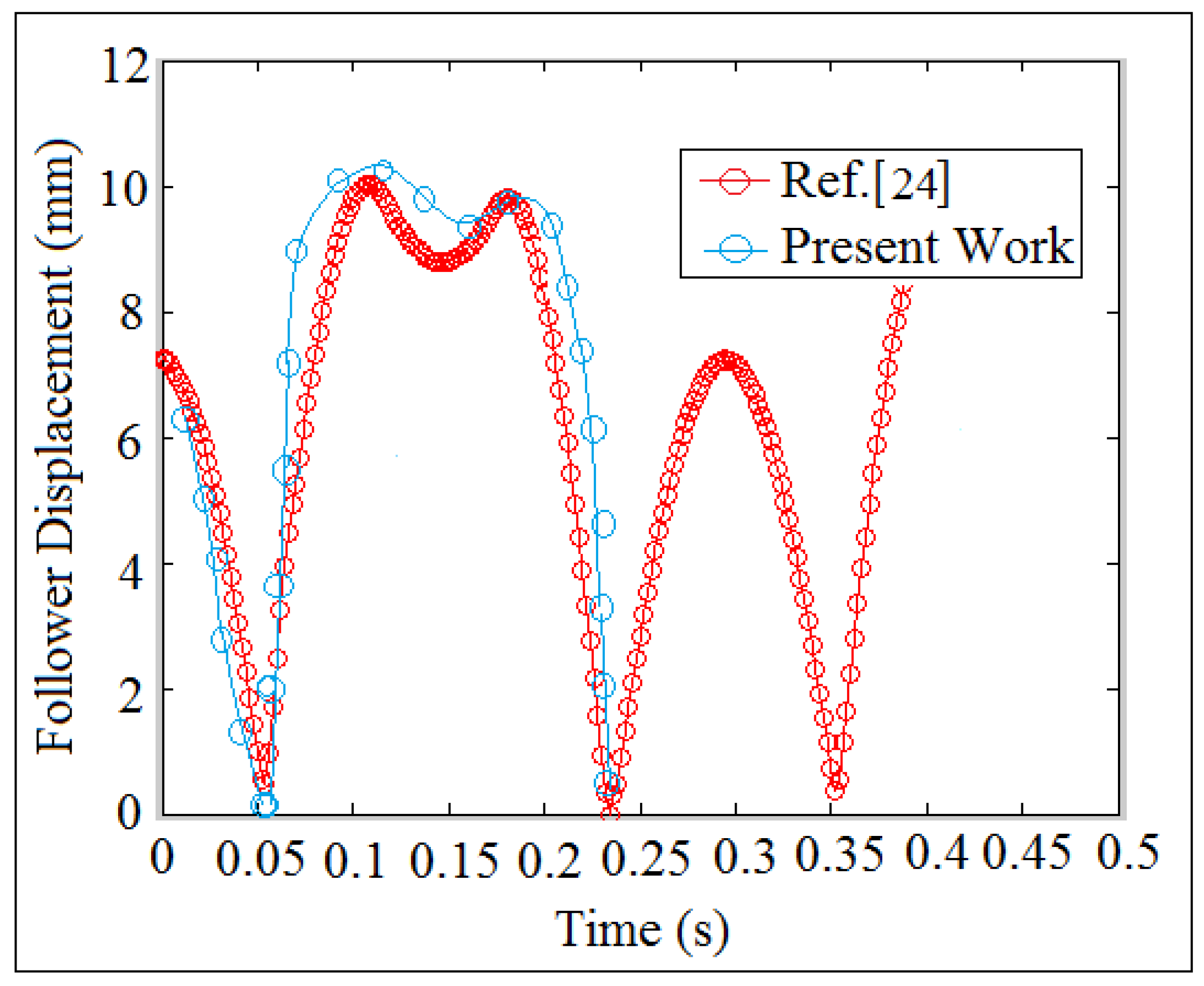
The analytic follower displacement was done by applying Equation (A13). Follower linear displacement was tracked experimentally through high speed camera at the foreground of OPTOTRAK/3020 equipment. Solidworks program was used in the numerical simulation of follower linear displacement. In the analytic solution of the follower displacement, the dwell stroke period of time was a straight line, which means that there was no detachment between the cam and the follower. In the numerical simulation, the dwell stroke was divided between the rise and return strokes and the detachment was intangible between the cam and the follower. In the experiment setup, the dwell stroke was tangible and it was varied sinusoidal against time. Regarding the comparison of the present work with the other publications, Figure 13 showed the comparison of nonlinear response of the follower against time. In the present work, the system with (I.D. = 17 mm) and (N = 200 rpm) was considered in the simulation using SolidWorks program. The author in Ref. [24] used six orders of piecewise polynomials for smoothing the motion curve of flat-faced follower due to the contact with a polydyne cam.
4.2. Detachment Detection through Contact Force
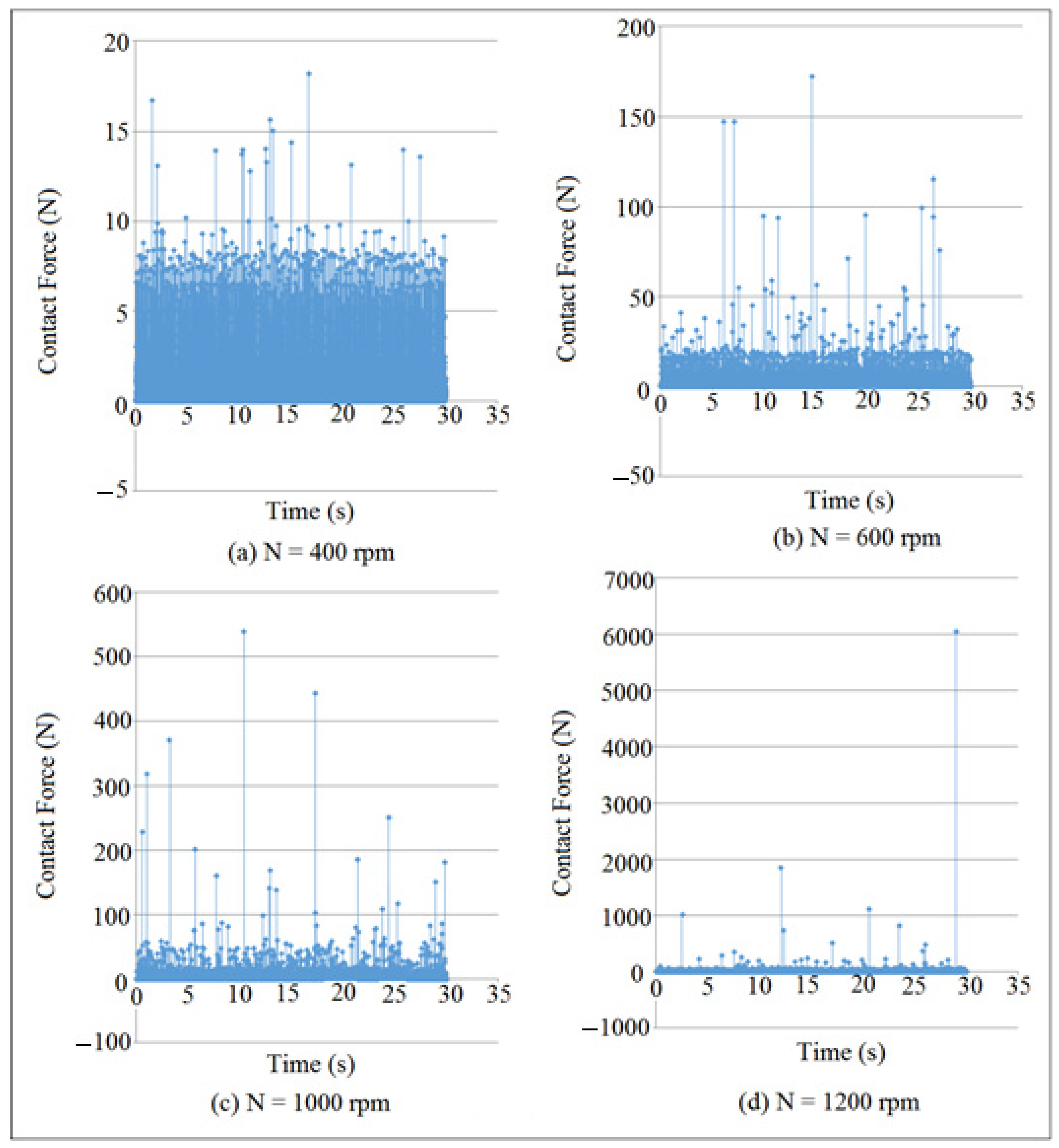
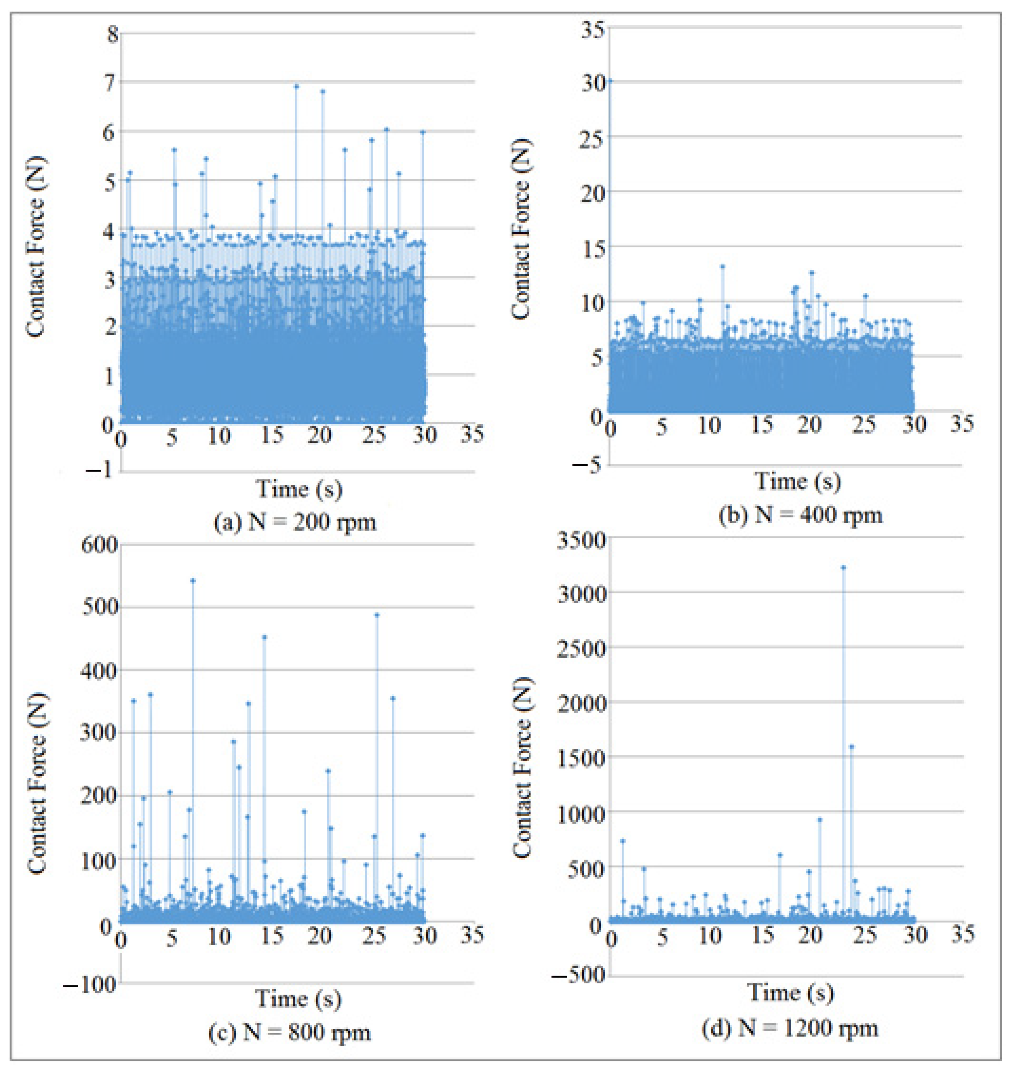
The weight of the follower was sufficient to maintain the contact when the follower moved with simple harmonic motion. Moreover, the preload spring between the installation table and the follower stem must be properly designed to maintain the contact. Figure 14 and Figure 15 showed the mapping of contact force against time for internal distance of the follower guide (I.D. = 16 and 17 mm) at different cam speeds (N). The detachment height was varied with the variation of the contact load value. The detachment occurred between the cam and the follower when the value of the contact force was in a minimum value, as indicated in Figure 14b–d and Figure 15b–d. There was an intangible detachment when the follower slipped off the cam as indicated in Figure 14a and Figure 15a at (N = 400 rpm and 200 rpm). In general, the detachments between the cam and the follower was increased when the contact force was in minimum value. SolidWorks program was used in the calculation of contact force at different (I.D.) and (N).
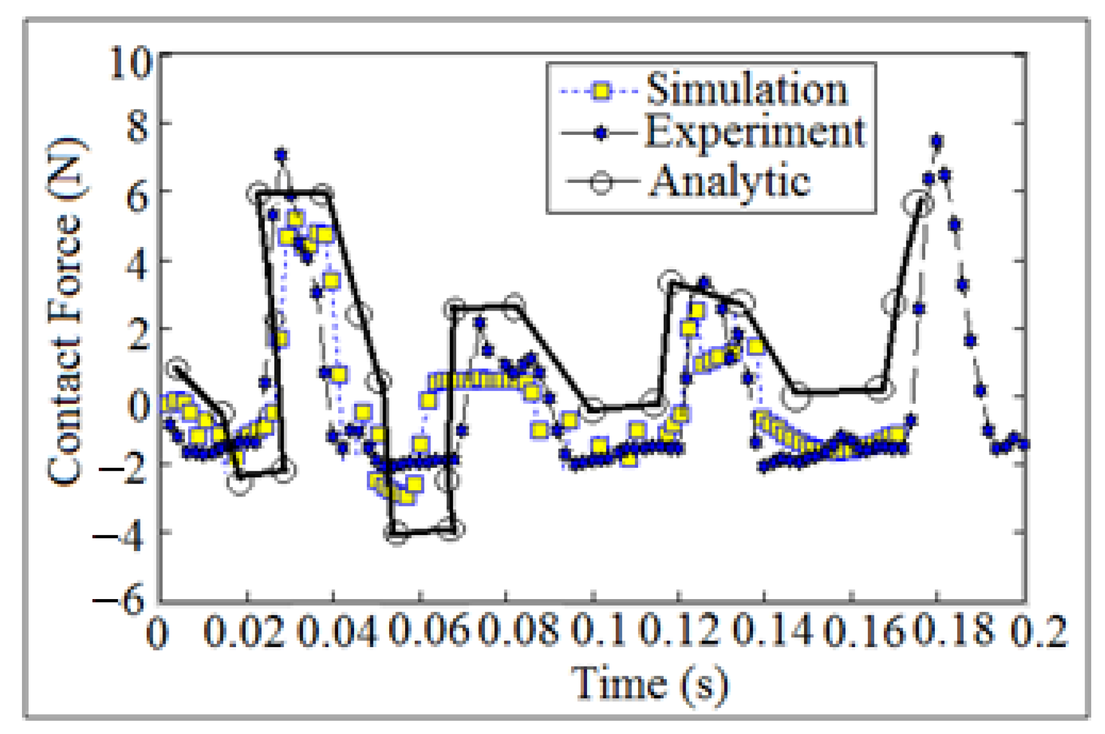
Figure 16 showed the comparison of the contact force against time at (I.D. = 16 mm) and (N = 200 mm). The analytic set of data of the contact force was calculated after applying Equation (A12), while the numerical simulation of the contact force was determined using SolidWoks program. The experimental set of data of the contact force was calculated after tracking the follower position using high speed camera at the foreground of the OPTOTRAK 30/20 equipment. Newton’s second law of dynamic motion was applied once and twice in the presence of follower mass and follower acceleration as mentioned earlier in (Experiment Test) section. In high speeds of the cam, it is important to produce a maximum acceleration which gives a negative value of the contact force. The follower acceleration is positive when the radius of curvature of the contact of the follower with the cam profile is positive and vice versa, [25]. Based on the above, the detachment between the cam and follower decreases when the follower decelerates at negative value for the contact force, especially at high speeds of the cam.
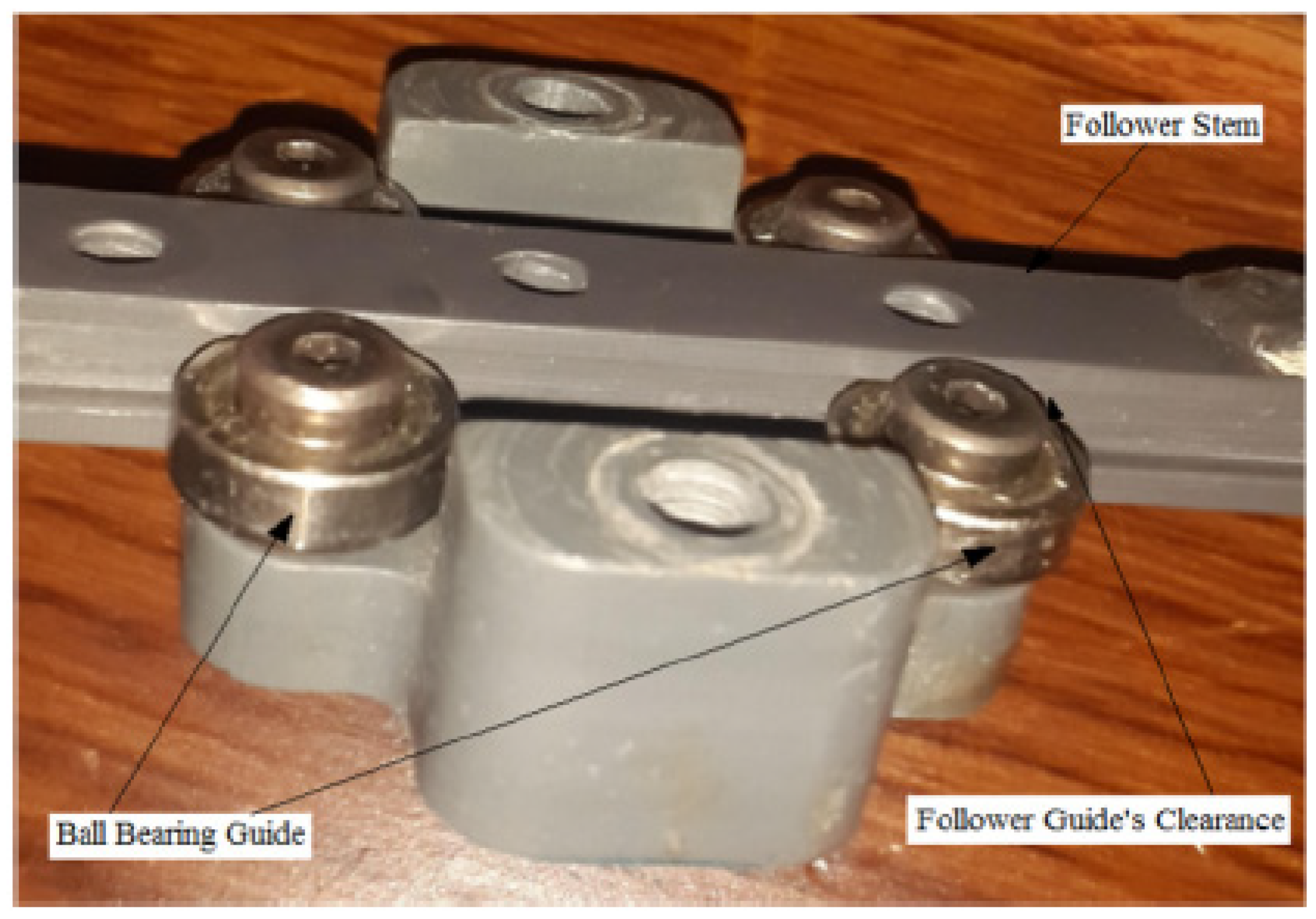
In this study, the detachment height of the follower was investigated in the presence of four internal distance of the follower guide from inside (I.D.) during the run of the numerical simulation analysis. In the experiment setup, the internal distance of the follower guide from inside was measured to be (I.D. = 16 mm) because it is constant from the manufacturer as shown in Figure 17.
5. Detachment Detection through Largest Lyapunov Exponent Parameter
Largest Lyapunov exponent parameter was used to detect the detachment in cam-follower system through the contact force. When the value of Lyapunov exponent of the contact force is positive, it means that there will be a detachment between the cam and the follower (non-periodic motion). Negative largest Lyapunov exponent value of the contact force indicates to periodic motion (the cam and the follower is in permanent contact) and the contact force has a maximum value. Wolf algorithm code based on MatLab software was used to extract the values of largest Lyapunov exponent by monitoring the orbital divergence for the contact force, [26]. Equations (5) and (6) were used to build Wolf algorithm code of the dynamic tool, [27].
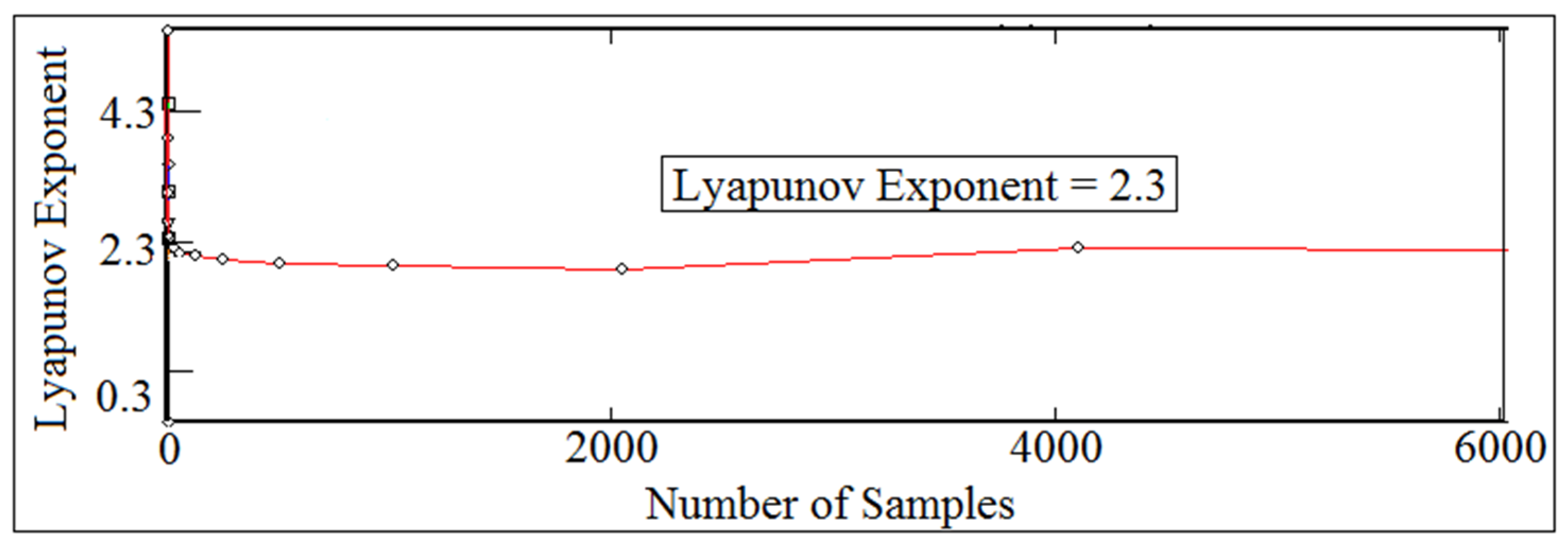
Figure 18 showed the numerical value of largest Lyapunov exponent against number of samples at (I.D. = 16 mm) and (N = 400 rpm). The value of Lyapunov exponent parameter was taken at its respective equilibrium point. One column of the contact force with the values of time delay and embedding dimension were used in Wolf algorithm to extract the numerical value of largest Lyapunov exponent parameter. One column of the contact force has been taken from the SolidWorks program where it was used in the dynamic tool of Wolf algorithm code. When the value of largest Lyapunov exponent is positive and above zero, it gives the indication that there will be a detachment between the cam and the follower.
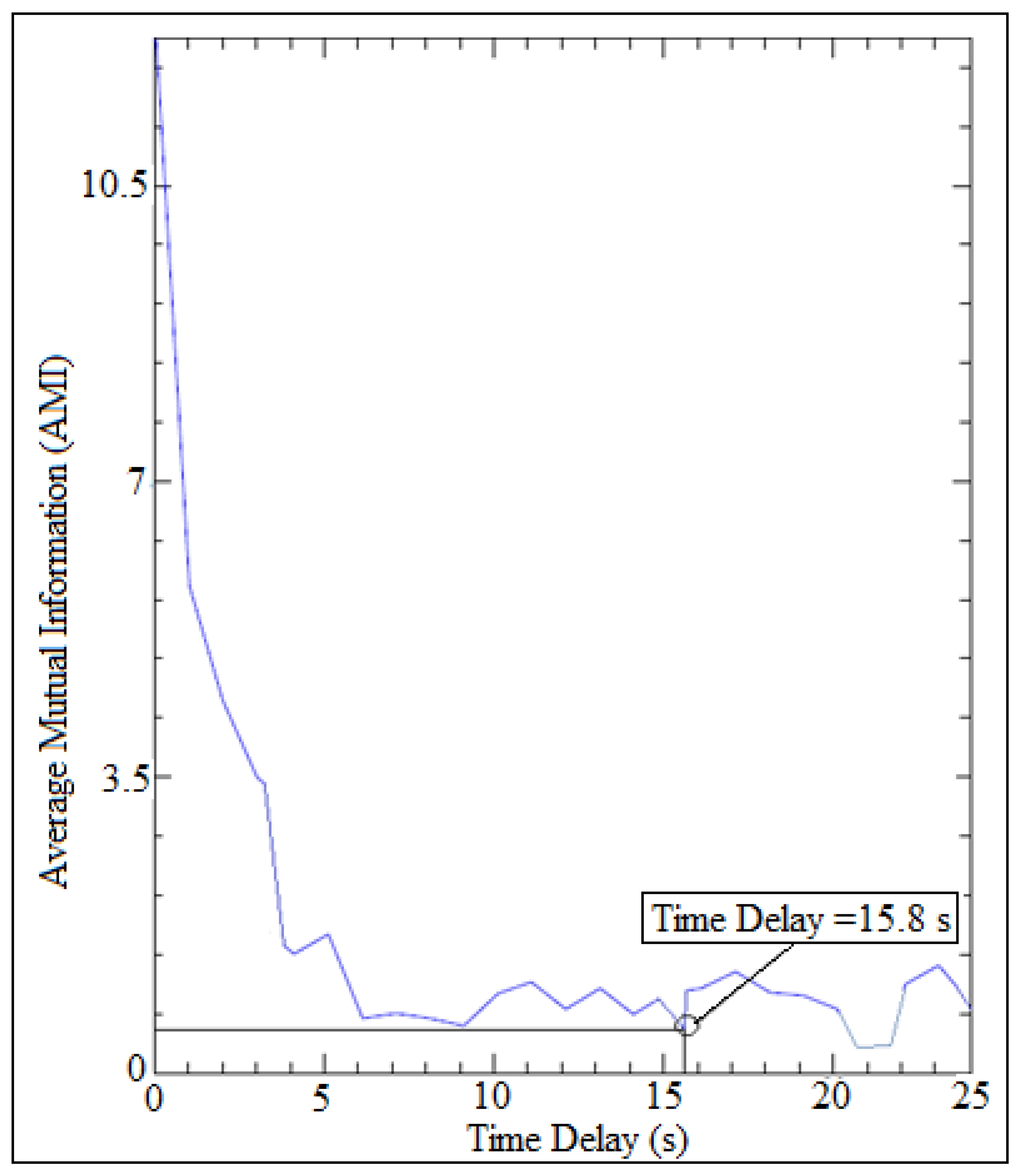
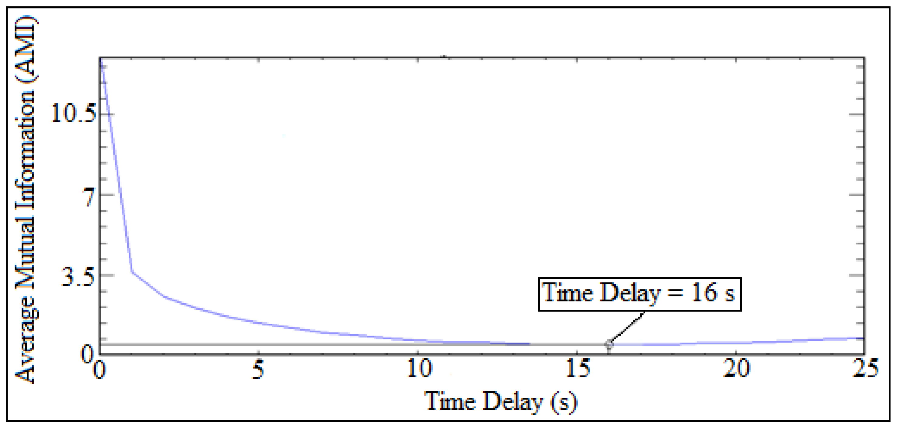
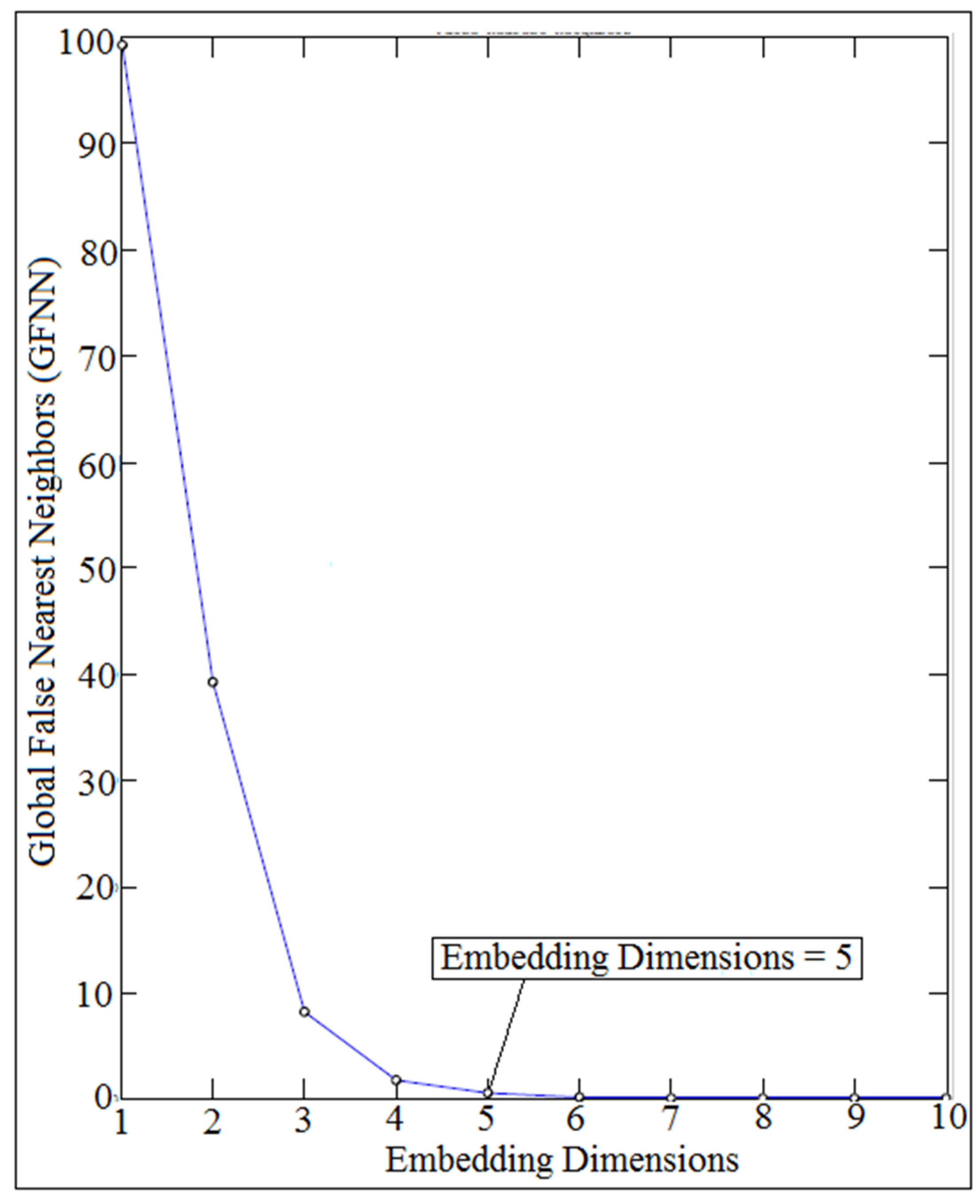
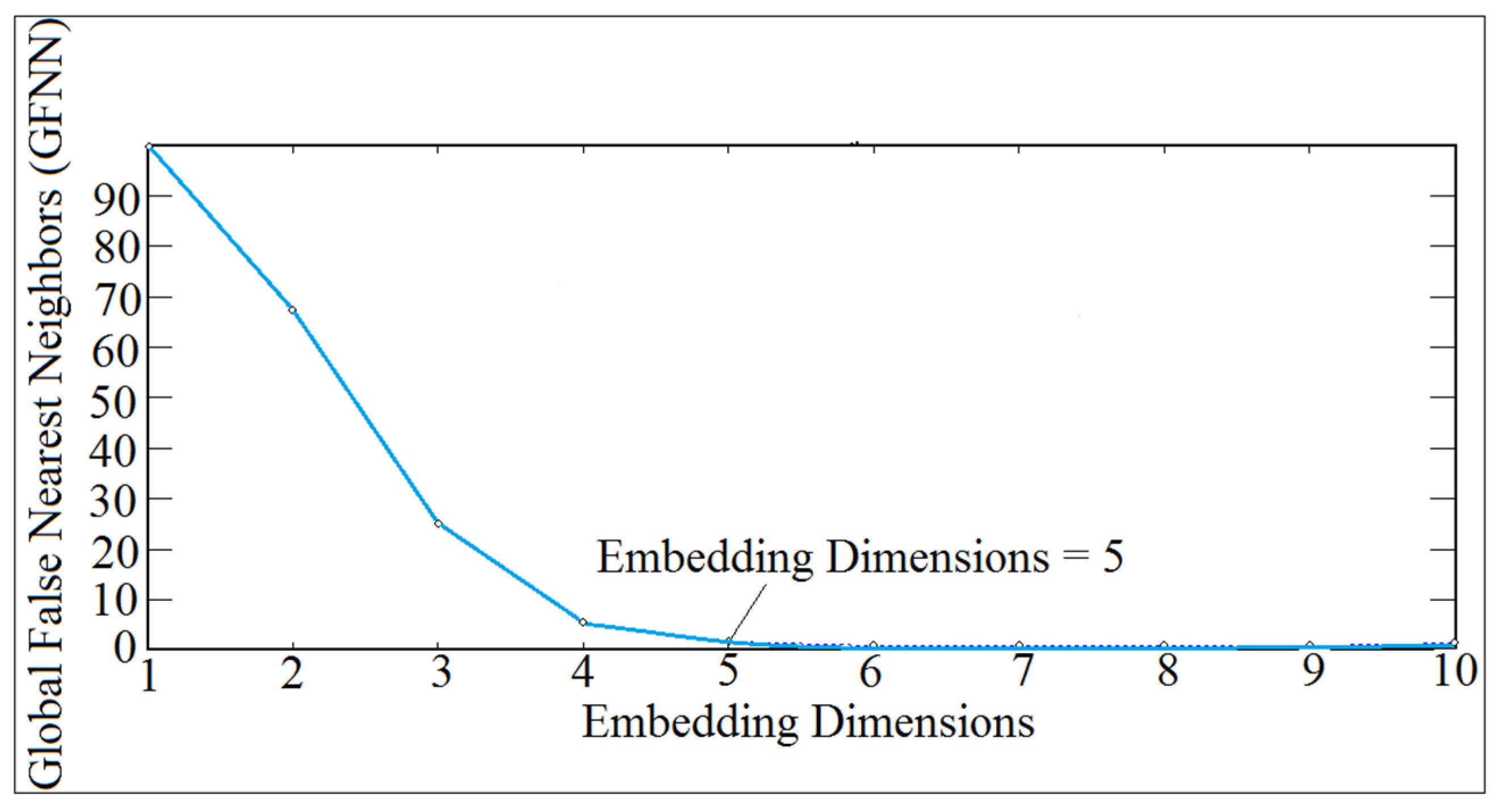
Time delay and embedding dimensions are numeric values in which it is needed in Wolf algorithm code in the estimation of local Lyapunov exponent Parameter. The algorithm of the dynamic code of global false nearest neighbors of the contact force was used to obtain the value of embedding dimensions in which it is estimated when the trend of global false nearest neighbors approaches zero, [28]. In this paper, a local and optimal time delay was estimated in which it is recommended that the local time delay should be chosen to be dependent on the embedding dimensions, [29]. The algorithm code of average mutual information was used to obtain the value of time delay and the first minimum time in the average mutual information trend represents the value of the time delay. The optimal time delay was calculated from the following equation:
where
- is the local time delay.
- is the optimal for independence of time series.
- P is the embedding dimensions.
Figure 19 and Figure 20 showed the comparison of time delay, while Figure 21 and Figure 22 showed the comparison of embedding dimensions.
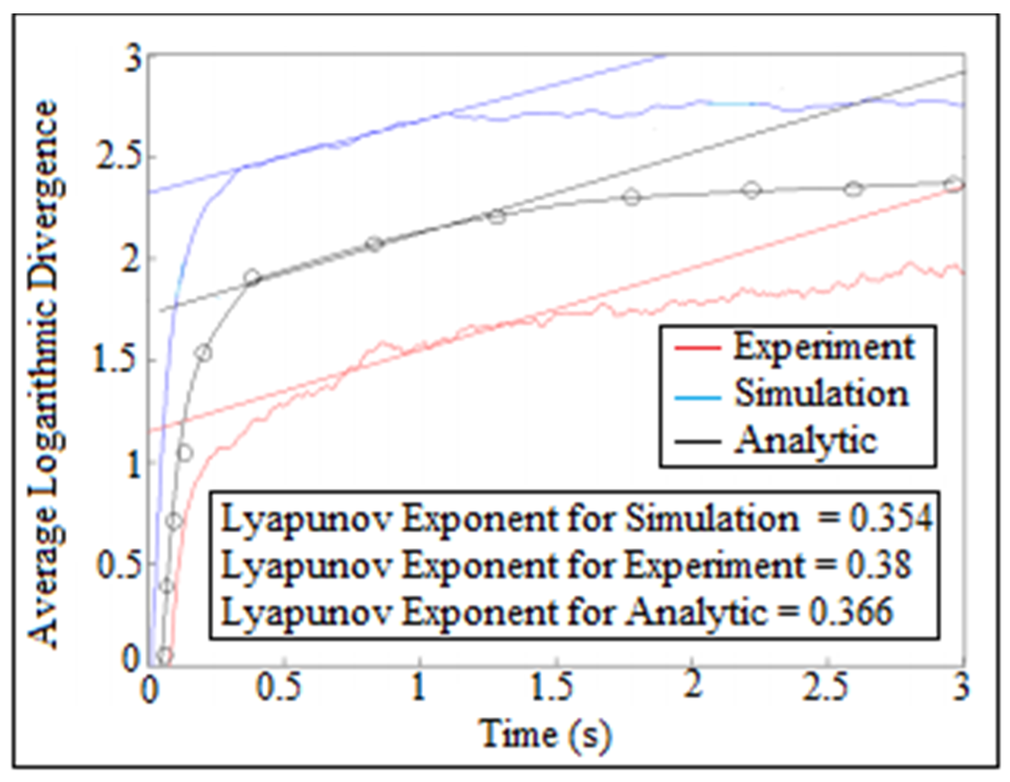
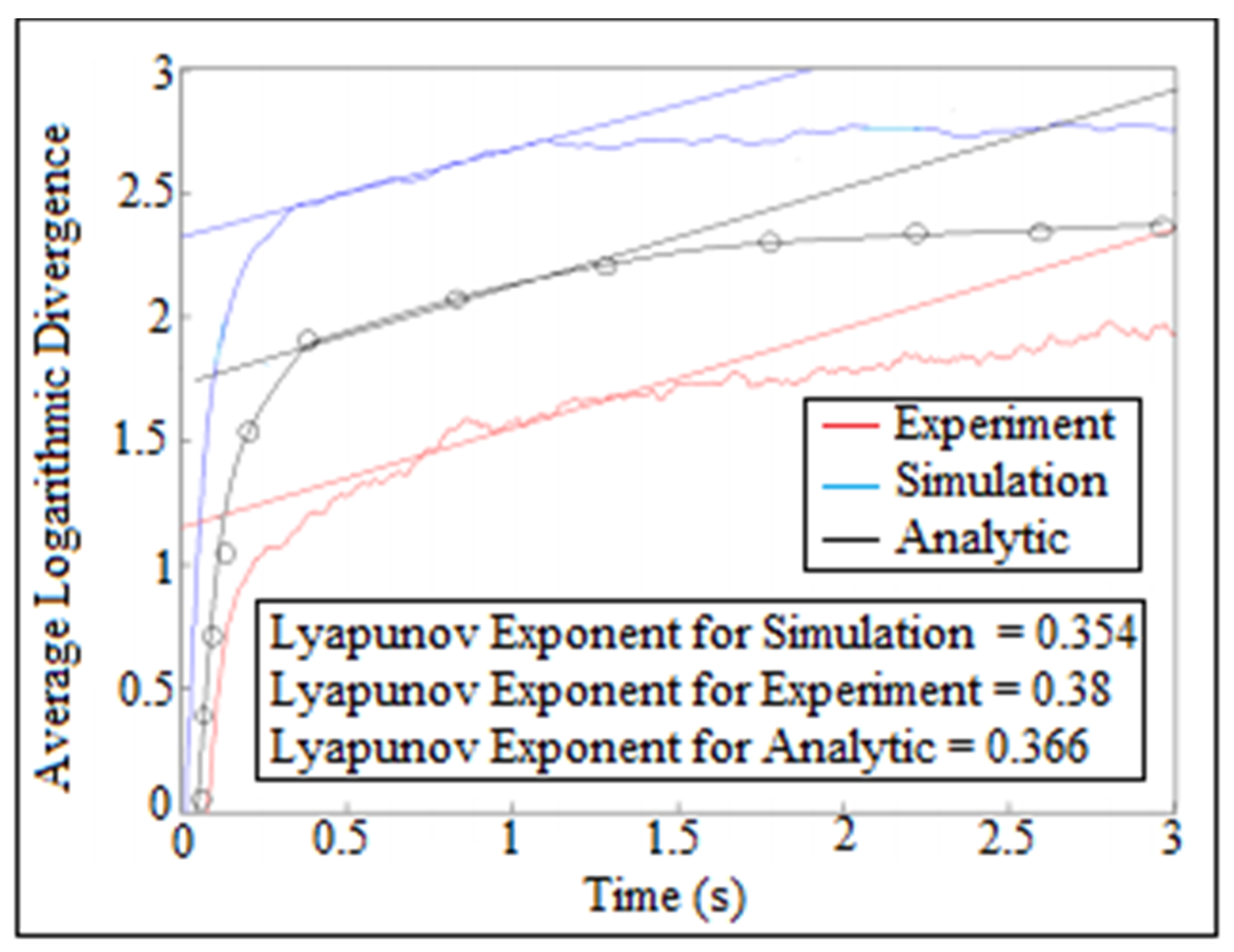
There was another way for estimating largest Lyapunov exponent of the contact force which was called average logarithmic divergence. The straight line represented the slope of average logarithmic divergence which reflected the value of Lyapunov exponent parameter. The curve represented the logarithm function against time of the contact force. As is known, the logarithm function treats any set of data by a straight line which gives the value of largest Lyapunov exponent. Figure 23 showed the comparison of average logarithmic divergence of contact force against time for (I.D. = 16 mm) and (N = 200 rpm). The analytic largest Lyapunov exponent of the contact force was calculated after applying Equation (A13) on one column of the contact force using average logarithmic divergence approach, while the numerical simulation of the largest Lyapunov exponent of the contact force was determined using SolidWoks program. The experiment value of largest Lyapunov exponent had been obtained after tracking the follower position using OPTOTRAK 30/20 equipment through high speed camera and by applying Newton’s second law of dynamic motion on the follower mass and follower acceleration as mentioned in (Experiment Test) section.
6. Detachment Detection through Fast Fourier Transform (FFT)
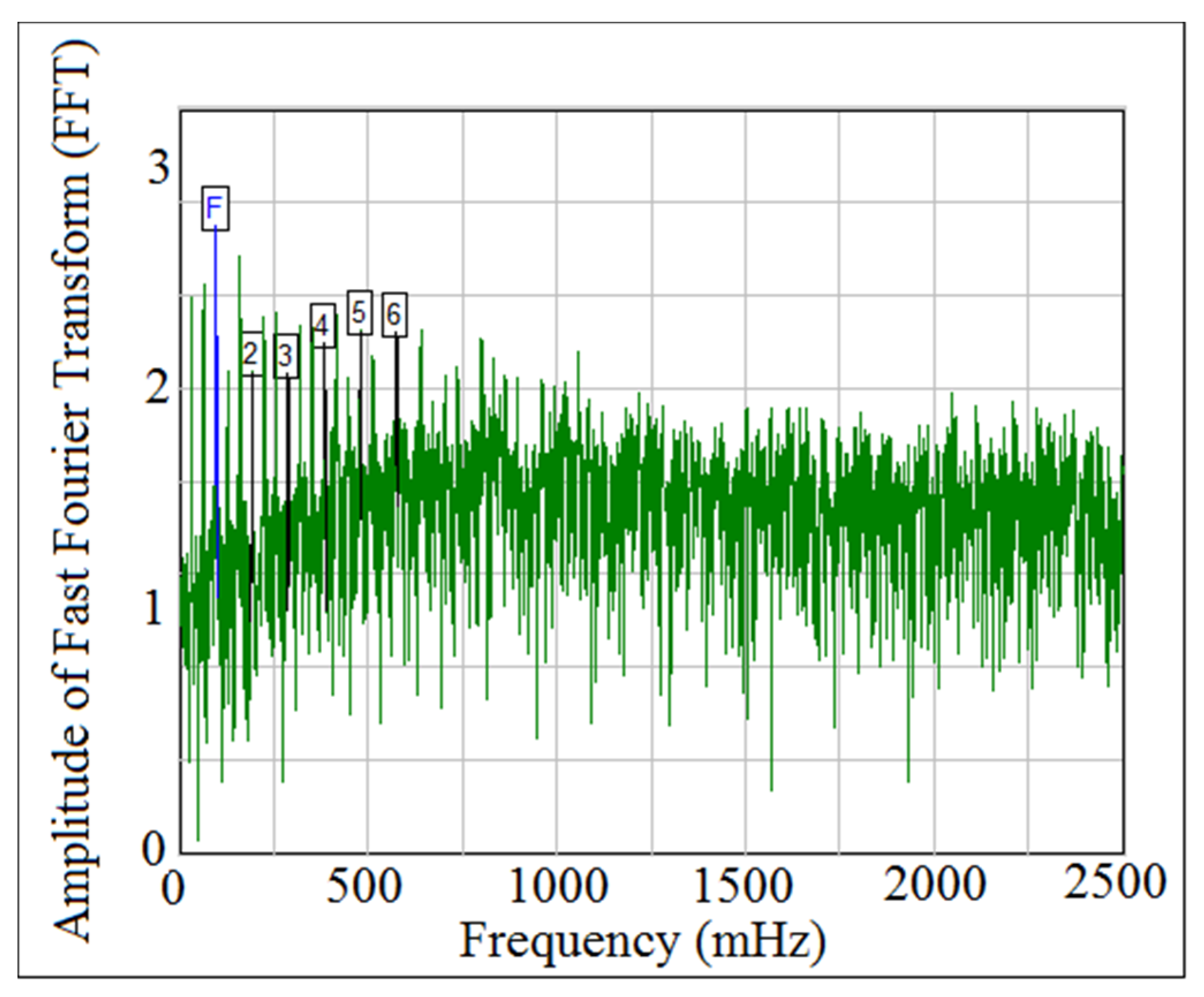
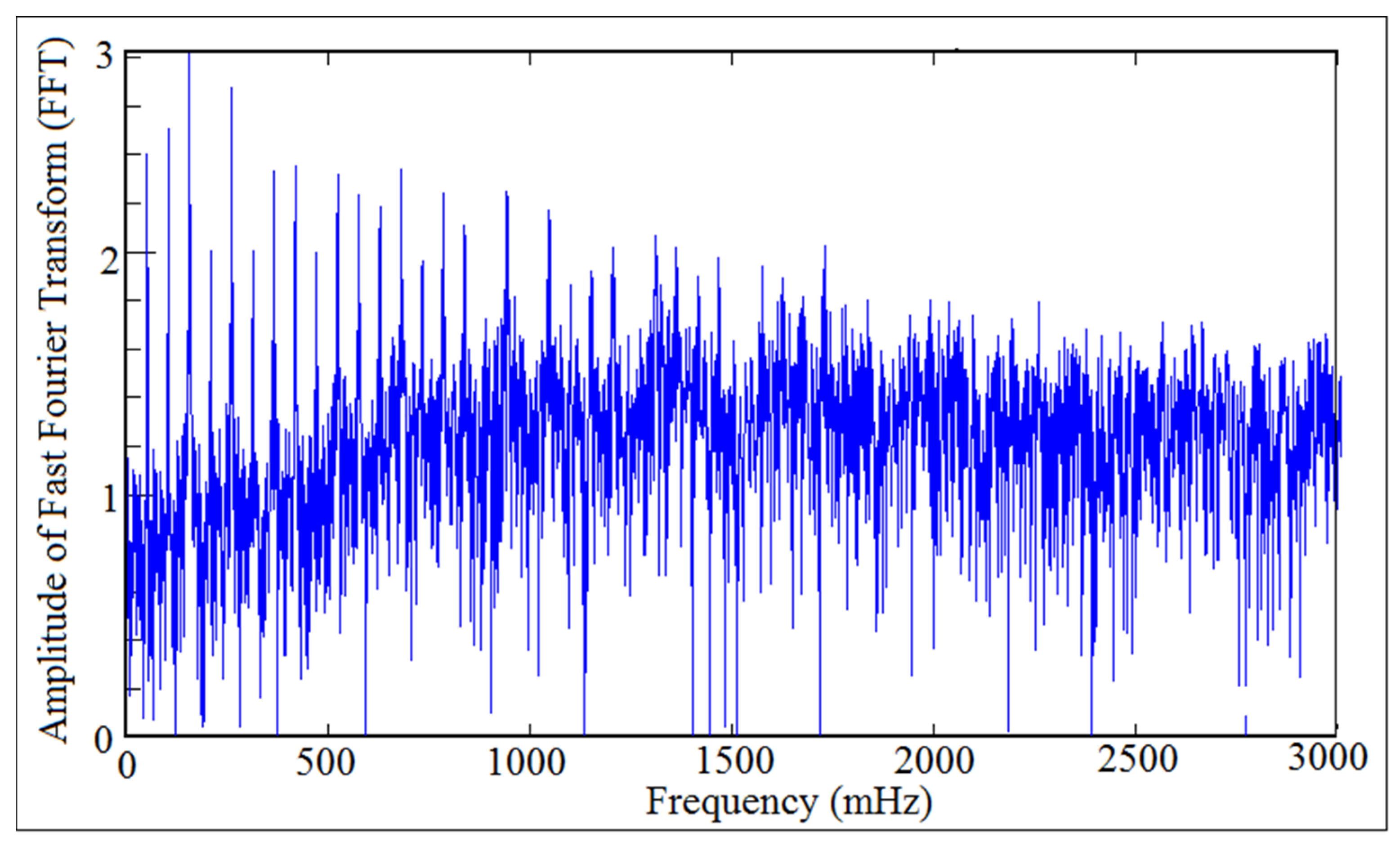
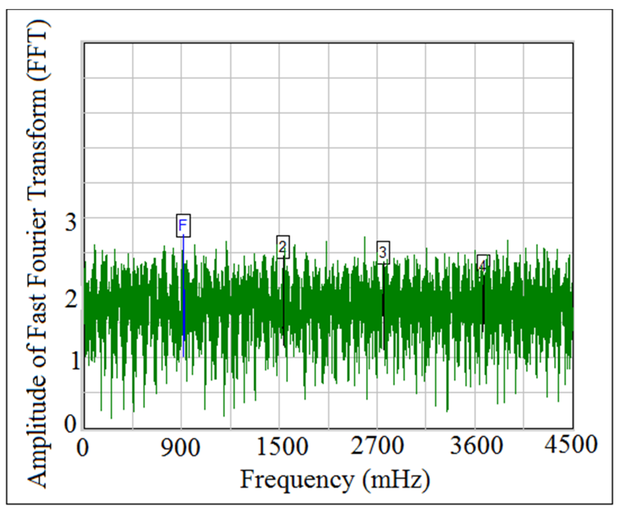
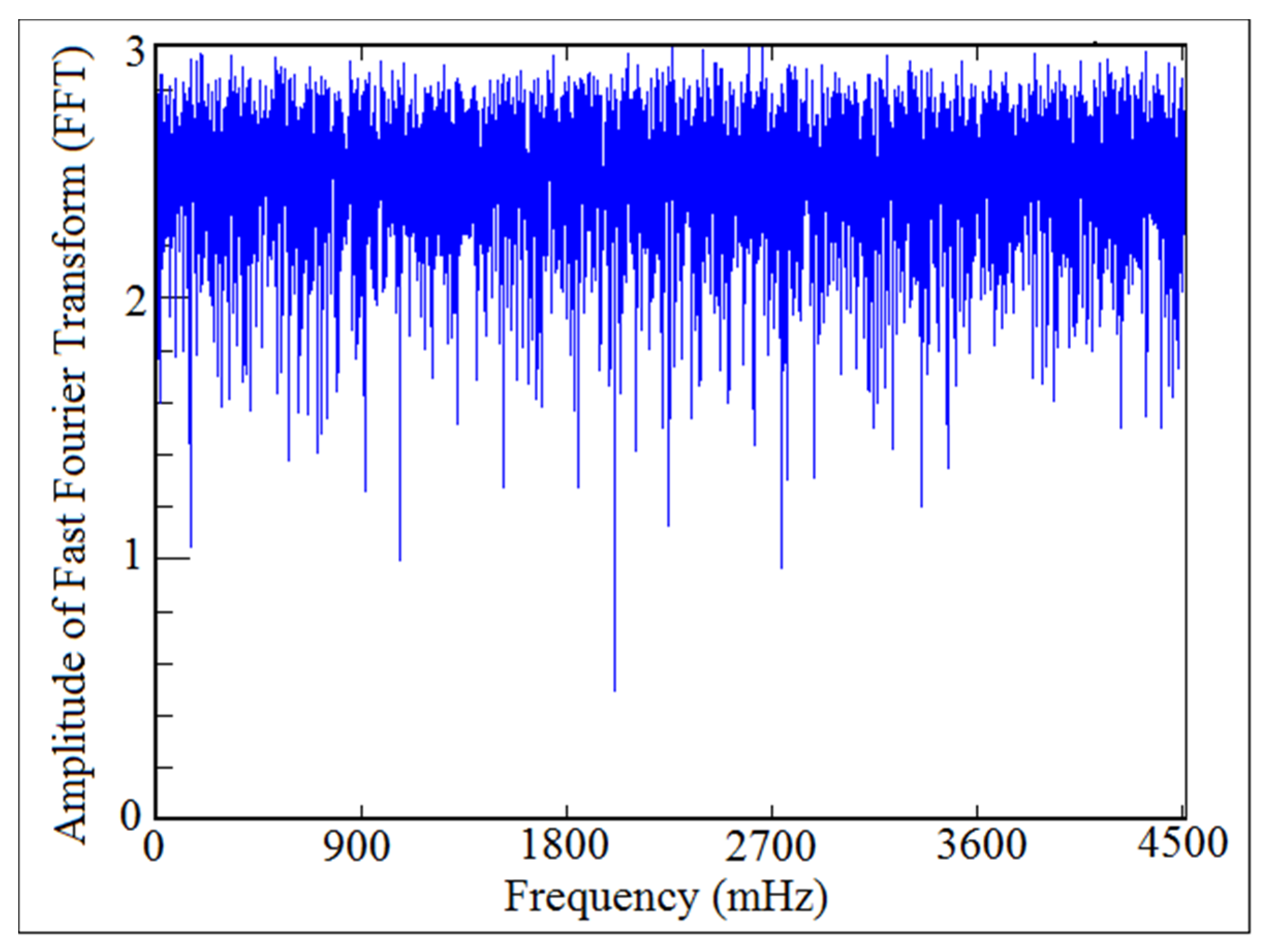
Power density function was used to detect the detachment between the cam and the follower because it gives six frequency peaks’ alongside with the fundamental frequency. [30]. The fundamental frequency has the letter (F), while the other frequencies’ peaks have the numbers (2, 3, 4, 5, 6) in (FFT) diagram. The peaks of the fundamental frequency and the other frequencies’ peaks refers to periodic motion (the contact force was in maximum value and there was no detachment between the cam and the follower). When the frequencies’ peaks have been started disappearing from (FFT) diagram, the motion is non-periodic (the contact force is approaching zero and the detachment between the cam and the follower is occurred). Figure 24 and Figure 25 showed the comparison of power spectrum analysis of Fast Fourier Transform (FFT) at (I.D. = 17 mm) and (N = 200 rpm). The numerical simulation values of the contact force was calculated using SolidWorks program, and after that, the one column of contact force was treated using (FFT). The experiment data of the follower displacement was tracked using OPTOTRAK 30/20 equipment through high speed camera and Newton’s second law of dynamic motion was applied based on the values of follower mass and acceleration to determine one column of the contact force. One column of the contact force was treated using (FFT). It can be concluded from Figure 24 and Figure 25 that there was no detachment between the cam and the follower because the six frequency peaks had not been disappeared from (FFT) diagram.
7. Detachment Detection through Poincare’ Map
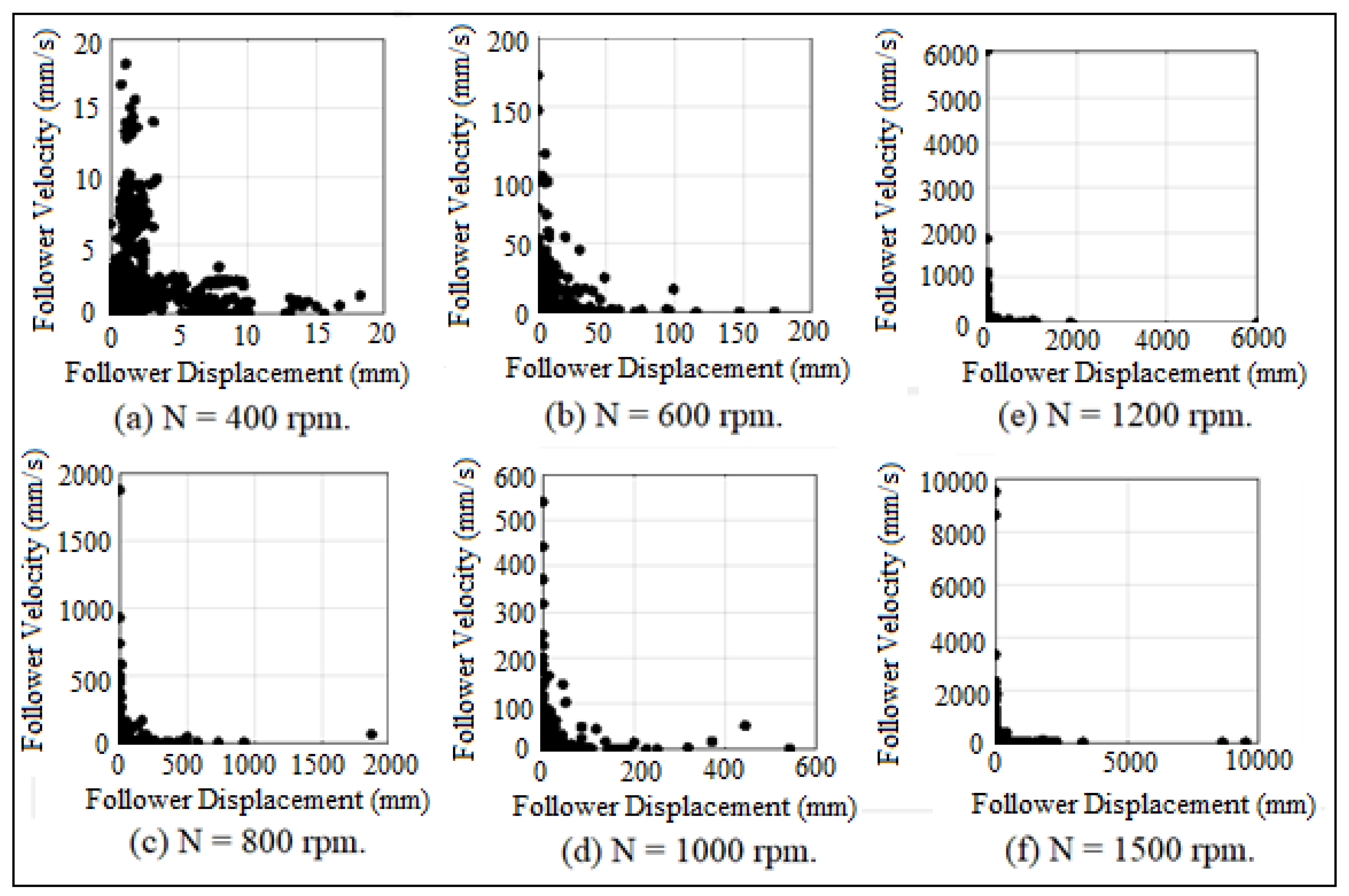
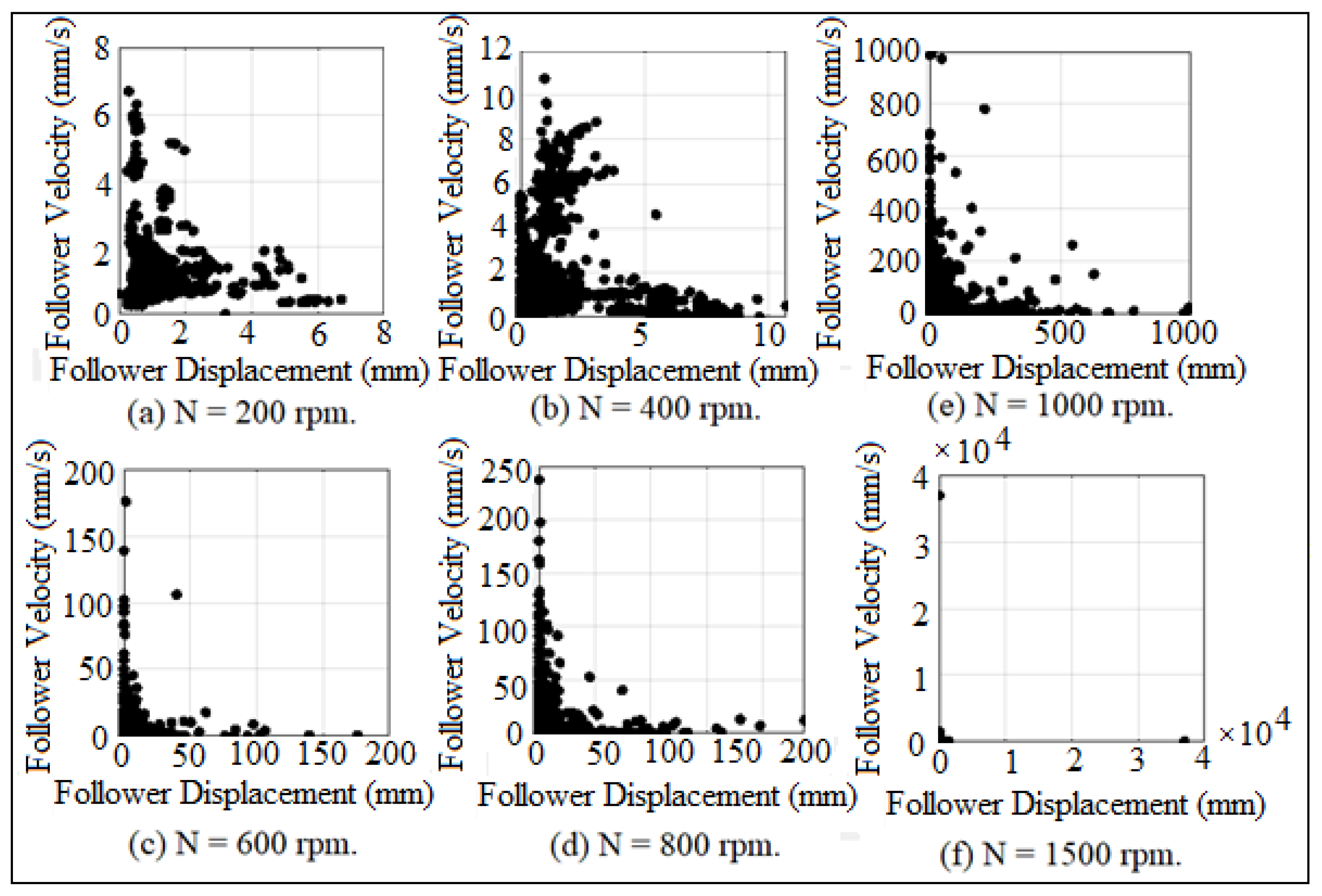
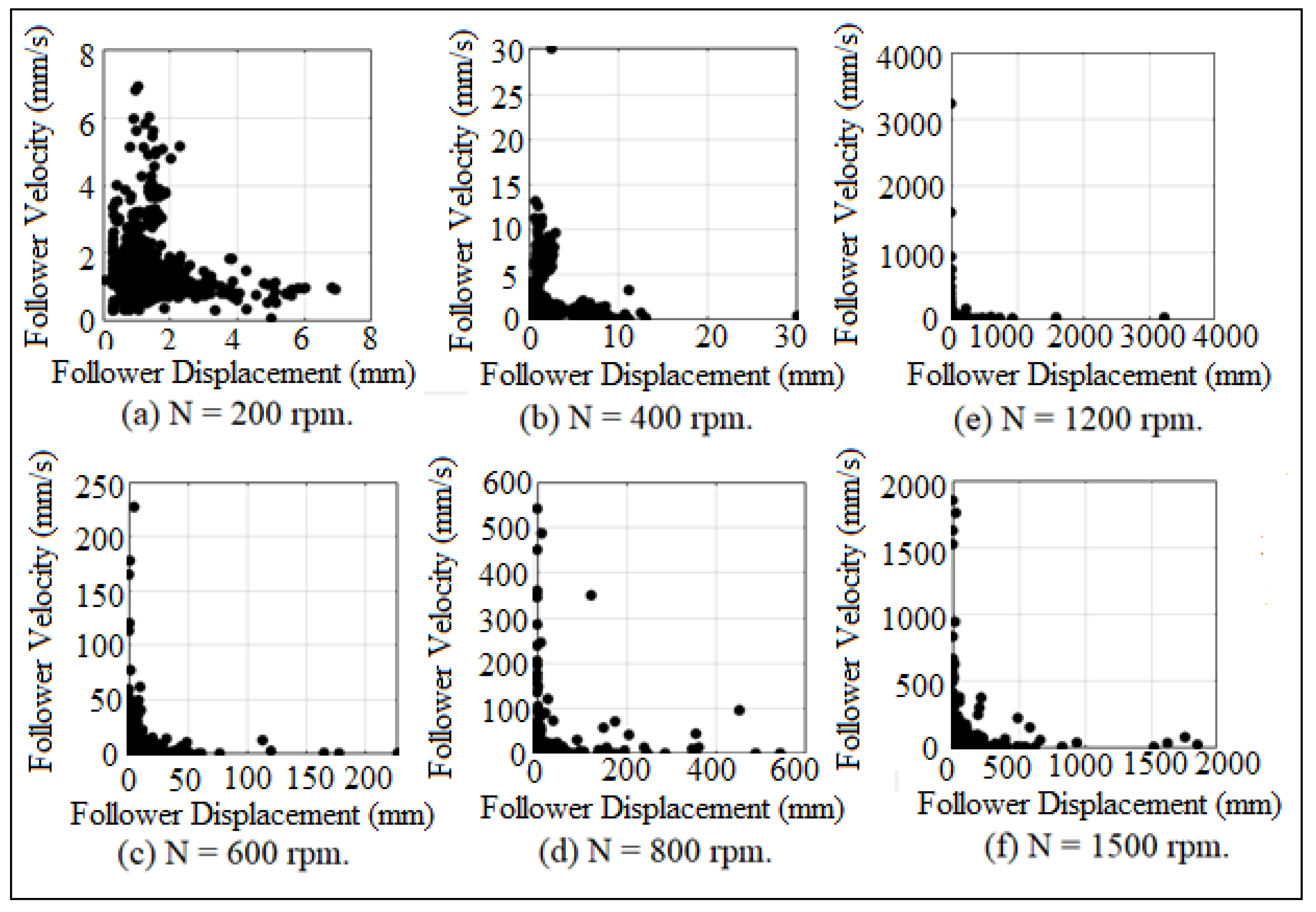
Poincare’ maps was used to investigate the periodicity of contact force diagram. Poincare’ map represents the records of the contact status between the cam and the follower. It is useful in identifying that either the follower is detached due to high speeds or it stays in permanent contact with the cam, [31]. Figure 26 and Figure 27 showed the mapping of Poincare’ maps for (I.D. = 16 and 18 mm) at different cam speeds (N). SolidWorks program was used in the simulation of Poincare’ maps. The more black dots, the more contact between the cam and the follower because the detachment is intangible when the follower either slips off or slides off the cam, as indicated in Figure 26a,b and Figure 27a,b,d,e. When the black dots started disappearing from Poincare’ maps, it means that the follower is detached from the cam profile, and the follower will start multi-impacts inside the cycle of the cam rotation, as shown in Figure 26e,f and Figure 27f.
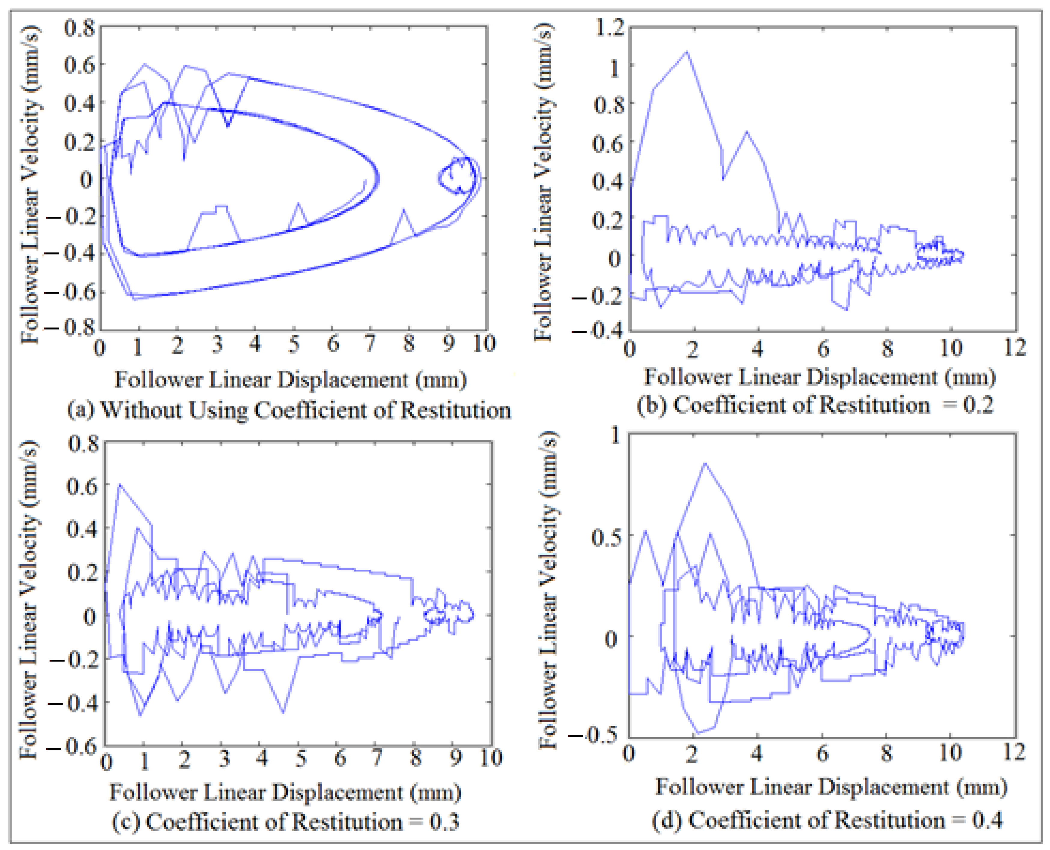
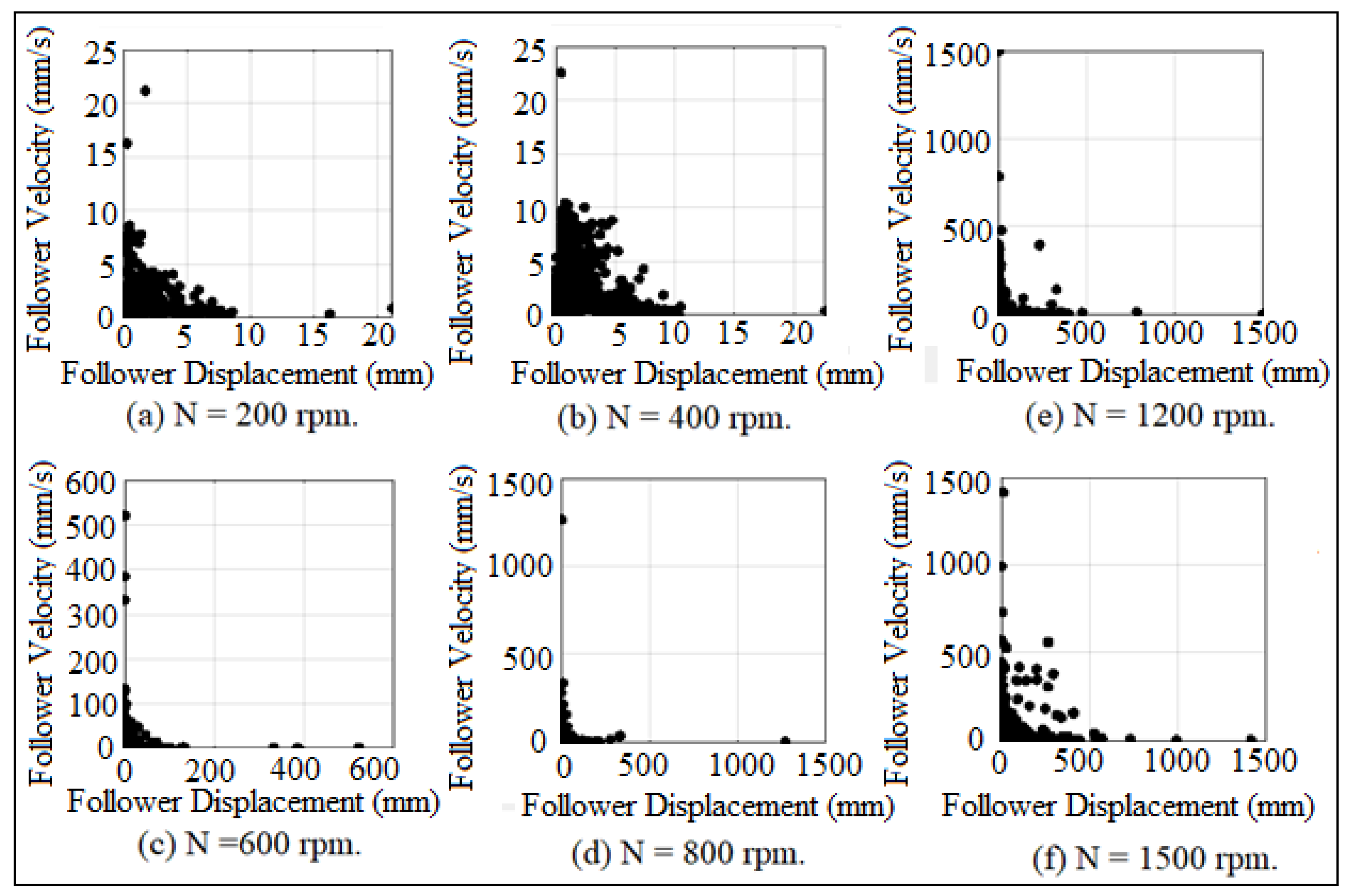
Phase-plane diagram works alongside with Poincare’ map to check for periodic and non-periodic motion of the follower movement. When the orbit of the follower movement is one closed curve which indicated to periodic motion but when the orbit of the follower movement diverges with no limits of spiral open cycles, it gives indication to non-periodic motion and chaos. Figure 28 showed the mapping of phase-plane diagram after using different values of coefficient of restitution at (I.D. = 19 mm) and (N = 200 rpm). The broken lines in the upper and lower surfaces in phase-plane diagram indicated to multi-impacts inside one cycle of the cam rotation as illustrated in Figure 28b–d. The broken lines in the upper and lower surfaces in the phase-plane diagram were increased with the increasing of coefficient of restitution values. The variation of the follower movement was increased with the increasing of coefficient of restitution values. Figure 28a showed the smooth contact between the cam and the follower at low speed (N = 200 rpm) without the use of coefficient of restitution parameter in which there was no broken lines in the upper and lower surfaces in the phase-plane diagram. SolidWorks program was used in the simulation of mapping of phase-plane diagram.
8. Results and Discussions
Figure 29 and Figure 30 showed the mapping of follower linear displacement against time at different cam speeds for (I.D. = 18 and 19 mm), respectively. There was no detachment between the cam and the follower as indicated in Figure 29a and Figure 30a, which means that the contact force has a maximum value. The detachment between the cam and the follower was increased with the increasing of cam angular velocities, which means that the contact force is approaching zero, as illustrated in Figure 29b–d and Figure 30b–d. Multi-detachments happened in one cycle of the cam rotation when the detachment heights were increased with the increasing of internal distance of the follower guide (I.D.) and cam speeds (N), as indicated in Figure 29c,d and Figure 30c,d. SolidWorks program was used in the numerical simulation of follower displacement.
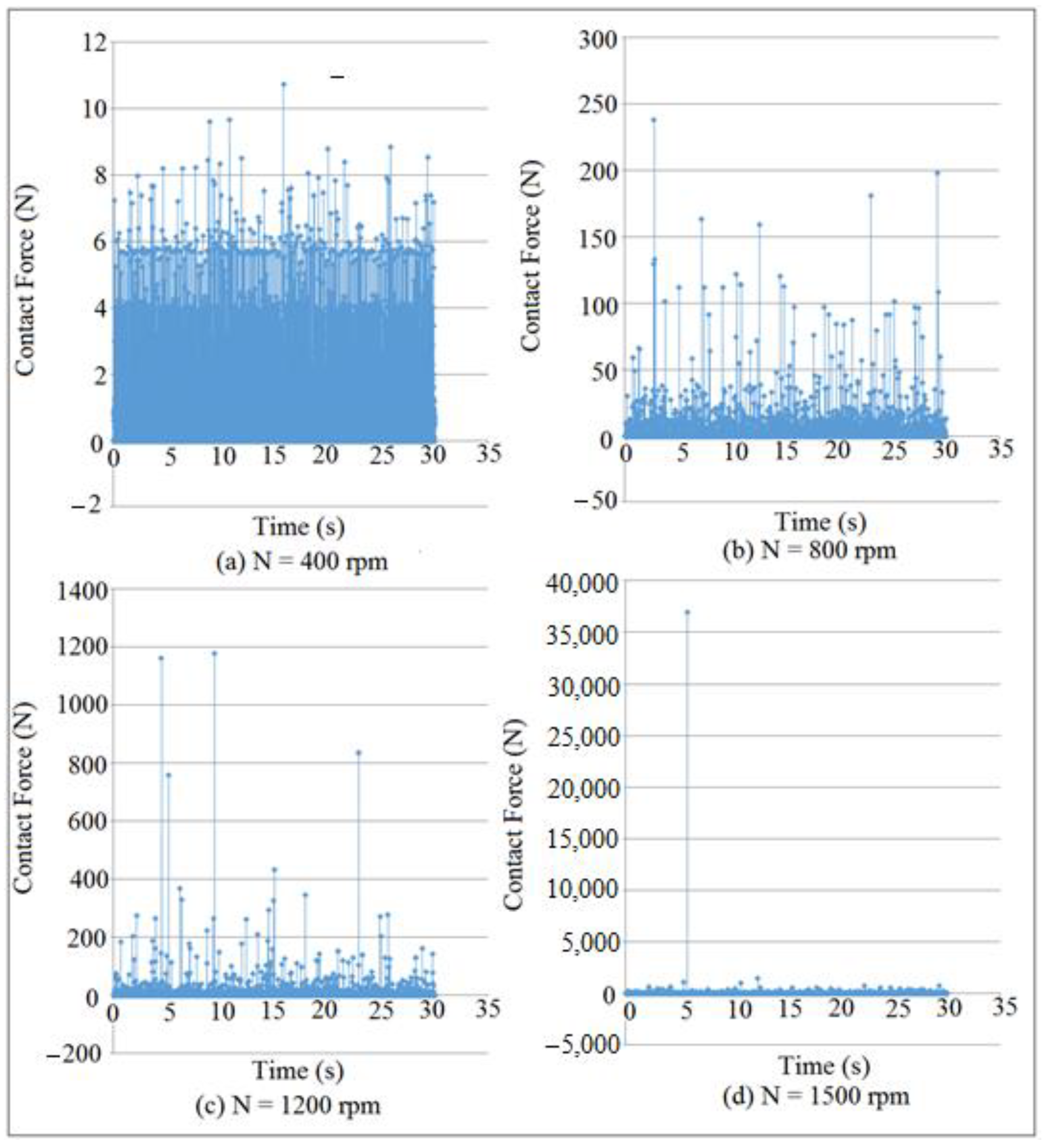
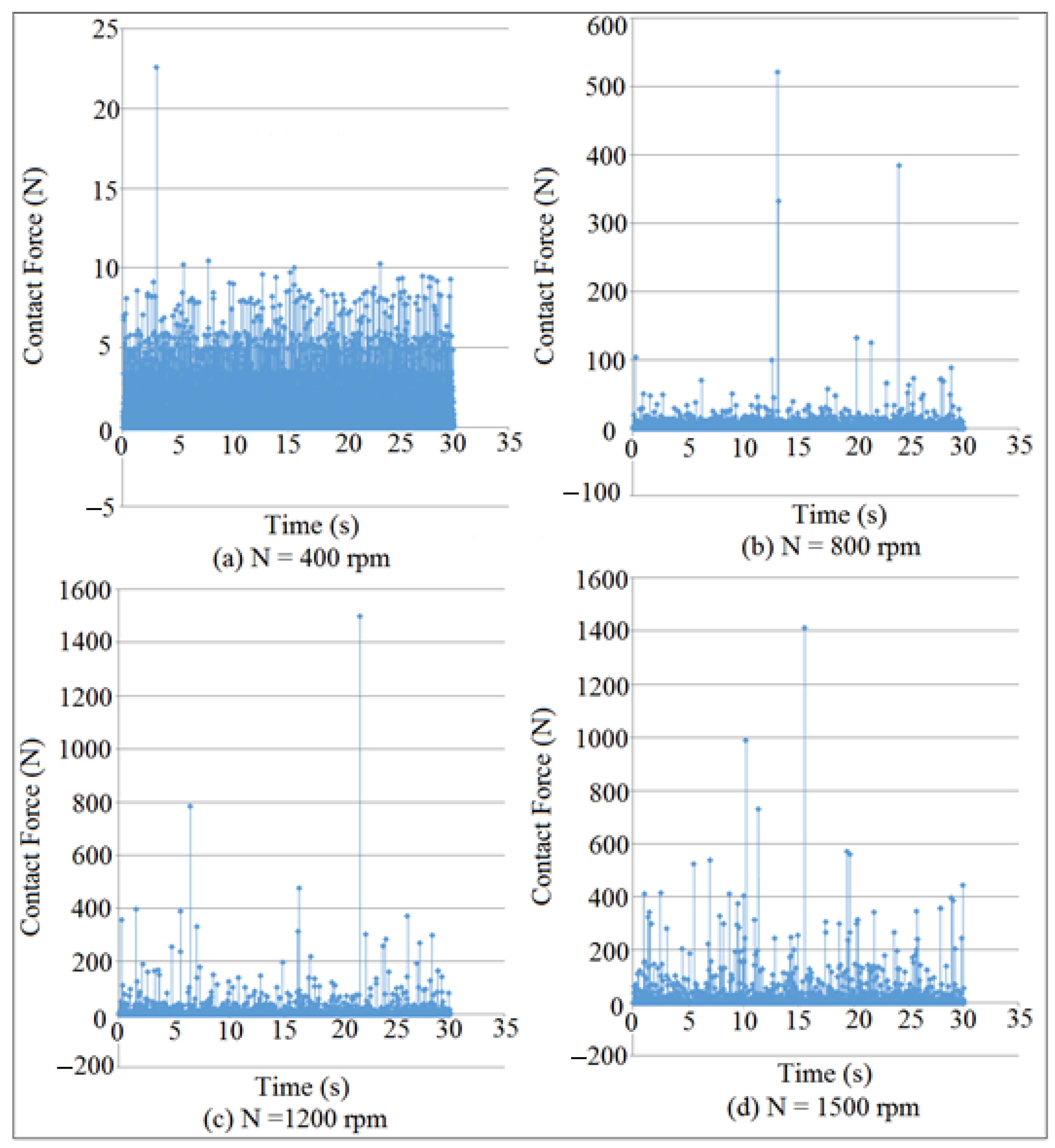
Figure 31 and Figure 32 showed the mapping of contact force at different cam speeds (N) and different internal distance of the follower guide (I.D.). The detachment occurred between the cam and the follower when the value of the contact force was in a minimum value, as indicated in Figure 31c,d and Figure 32b,c. The value of the contact force had declined with the increasing of cam speeds and internal distance of the follower guide. The system with (I.D. = 18 mm) and (N = 1500 rpm) has a minimum value of contact force (multi-detachment heights happened in one cycle of the cam rotation). SolidWorks program was used in the simulation of the contact force.
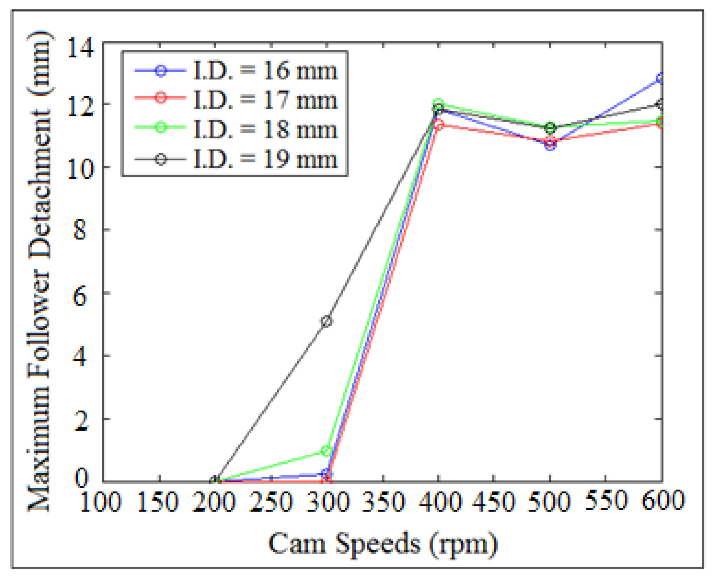
Figure 33 showed the maximum detachment heights of the follower against cam speeds at different internal distance of the follower guide (I.D.). The maximum detachment height of the follower was increased with the increasing of cam speeds. The detachment height of the follower was in a minimum value at (N = 200–300 rpm) and (I.D. = 16, 17, and 18 mm). There was no detachment between the cam and the follower at (N = 100–200 rpm) for all internal distance of the follower guide (I.D.), which means that the contact force has a maximum value (no separation between the cam and the follower will occur). SolidWorks program was used in the simulation of the follower displacement.
Figure 34 and Figure 35 showed the comparison of power density function of Fast Fourier Transform (FFT) of the contact force at (I.D. = 19 mm) and (N = 400 rpm). It can be concluded from Figure 34 and Figure 35 that there was detachment between the cam and the follower since the six frequency peaks have disappeared from the (FFT) diagram when the contact force approaches zero.
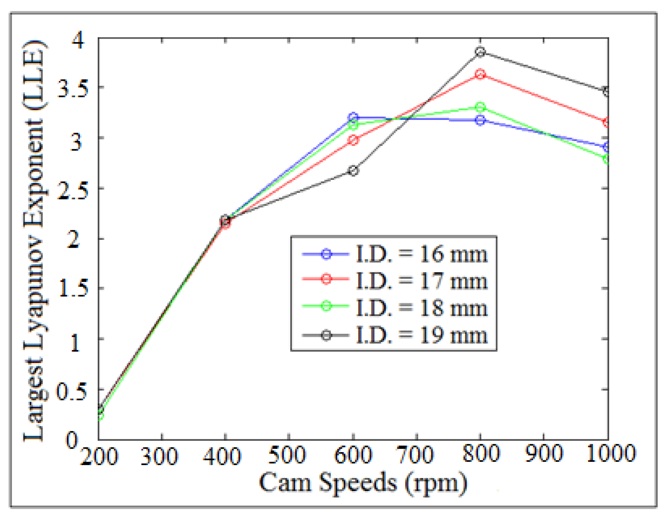
Figure 36 showed the largest Lyapunov exponent against cam speeds at different internal distance of the follower guide (I.D.). The values of largest Lyapunov exponent of the contact force were increased with the increasing of cam speeds. The values of (LLE) for all the systems were the same at N = (200–400 rpm), while (LLE) was varied with sinusoidal against cam speeds at (N = 400–1000 rpm). The value of Lyapunov exponent parameter was taken at its respective equilibrium points. The value of largest Lyapunov exponent was above zero and was positive, which gives indication that there was a detachment height between the cam and the follower. SolidWorks program was used in the numerical simulation of the contact force.
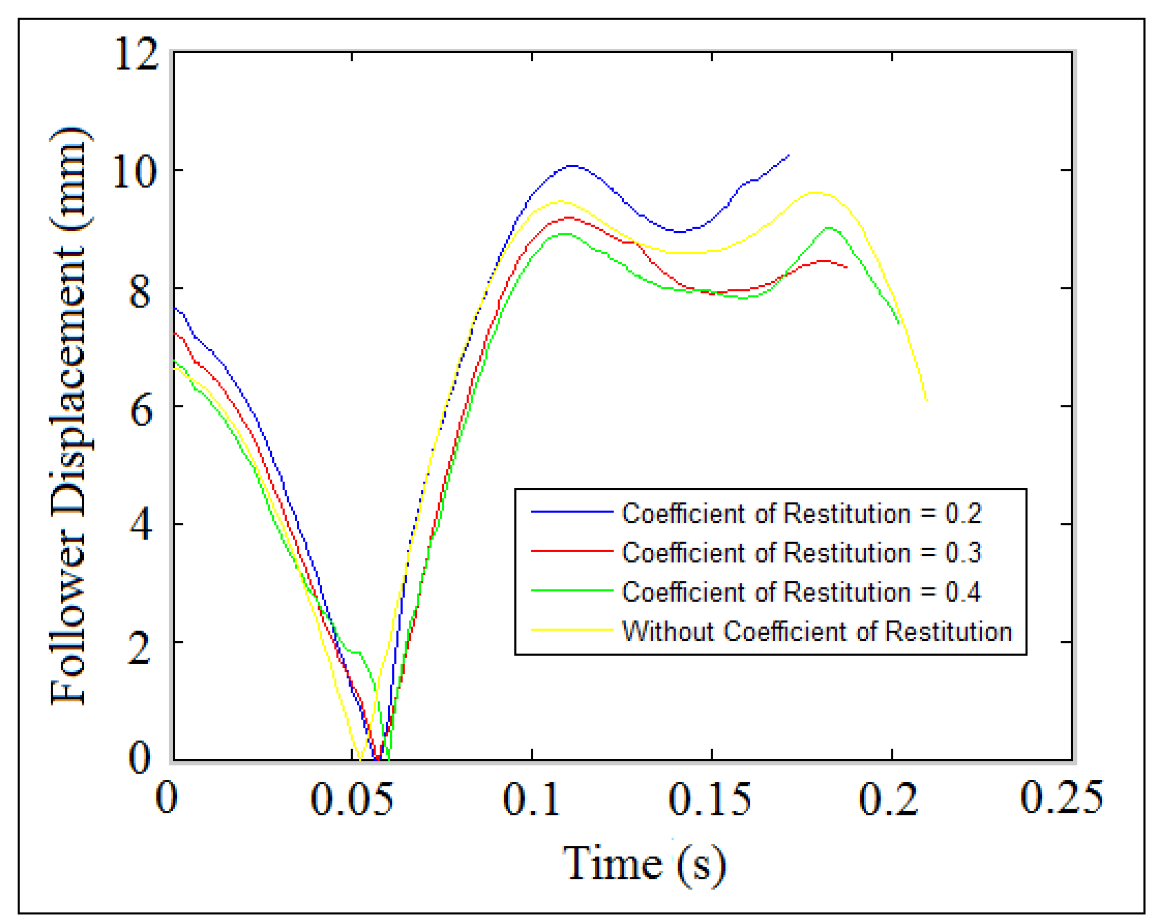
Figure 37 showed the behavior of the follower displacement against time for different values of coefficients of restitution. The peak of the follower displacement was decreased with the increasing of coefficients of restitution because the potential energy of the follower has declined and dissipated due to the impact. There was no loss in potential energy because both the cam and the follower were in permanent contact with no effect of the coefficient of restitution.
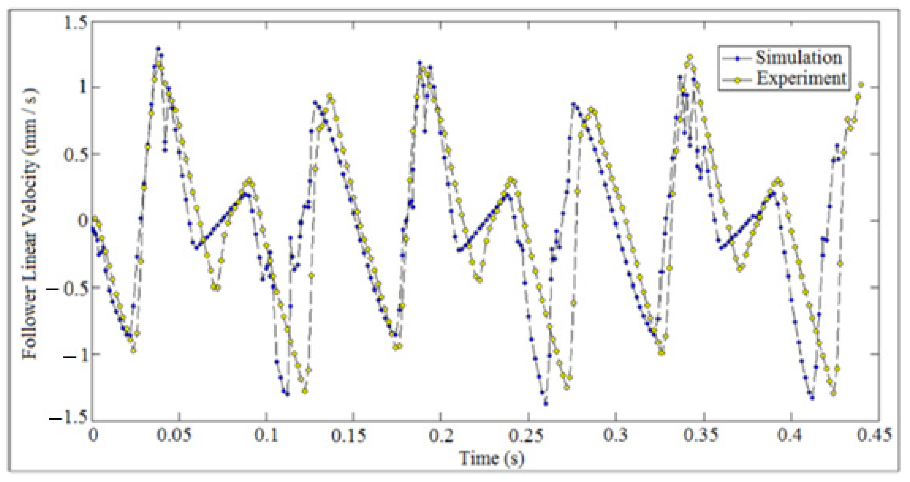
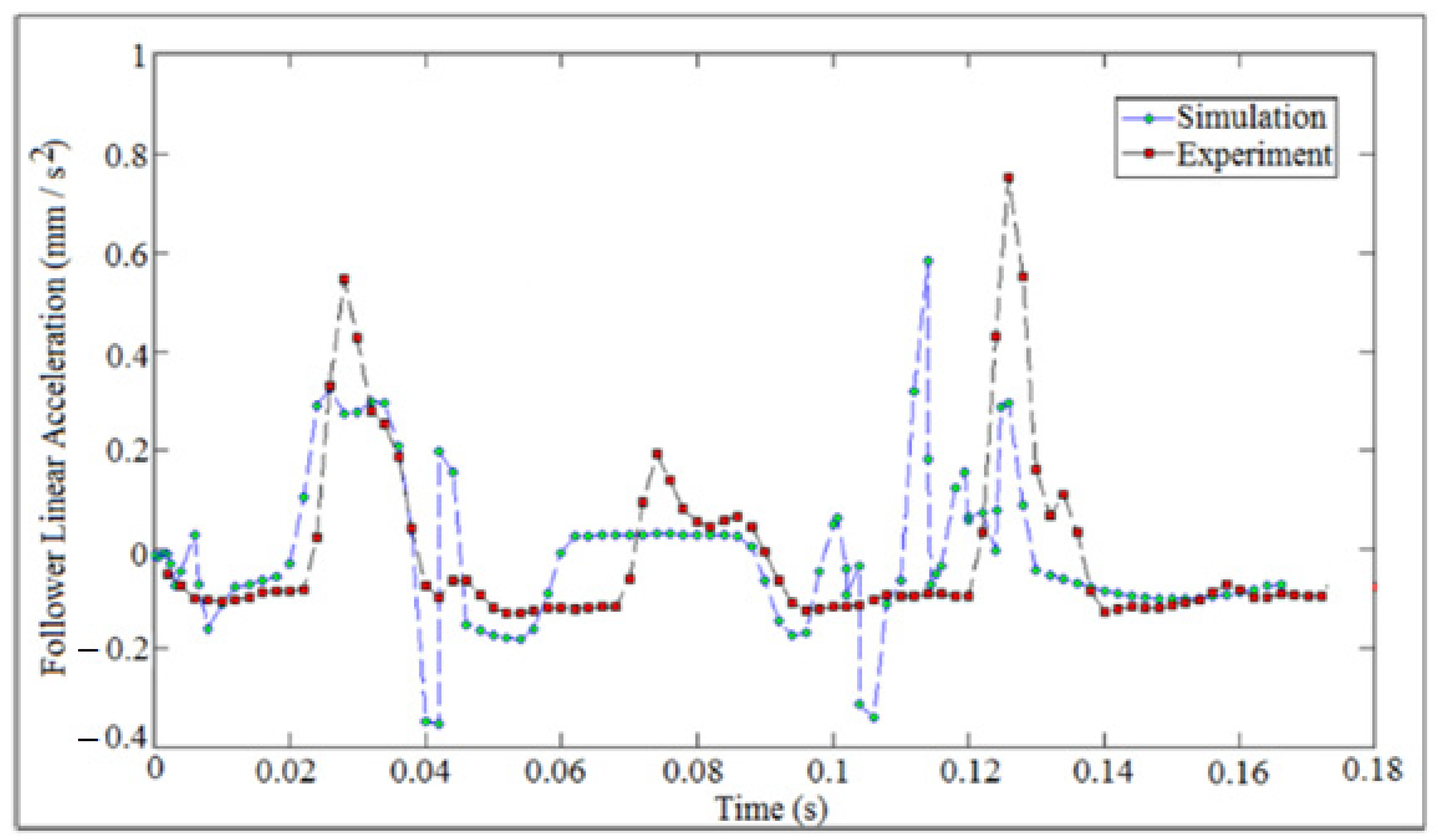
Figure 38, Figure 39 and Figure 40 showed the comparison of follower linear displacement, velocity, and acceleration against time for (I.D. = 16 mm) and (N = 200 rpm). The experiment set of data of the follower displacement was tracked using a high speed camera at the foreground of the OPTOTRAK 30/20 equipment, and the follower displacement was derived once and twice to determine follower velocity and acceleration, respectively.
Figure 41 and Figure 42 showed the Poincare’ maps of the contact force for different internal distance of the follower guide (I.D.) and different cam speeds (N). SolidWorks program was used in the simulation. The more black dots, the more contact between the cam and the follower in which the detachment was intangible. The follower had slipped off the cam, as indicated in Figure 41a,b and Figure 42a,b,f. When the black dots started disappearing from Poincare’ maps, it meant that the follower was detached from the cam profile and started multi-impacts inside one cycle of the cam rotation, as shown in Figure 41c,e and Figure 42c,d.
Figure 43 showed the average logarithmic divergence of contact force against time for (I.D. = 18 mm) and (N = 200 rpm), respectively. The experiment results of Lyapunov exponent was carried out through high speed camera which was located at the foreground of the OPTOTRAK 30/20 equipment by tracking the follower position, and I used them as a one column of follower position with time delay and embedding dimension in Wolf algorithm code. The analytic value of Lyapunov exponent was done by calculating one column of the contact force after applying Equation (A12), while the numerical simulation value of Lyapunov exponent was determined based on one column of the contact force from SolidWorks program.
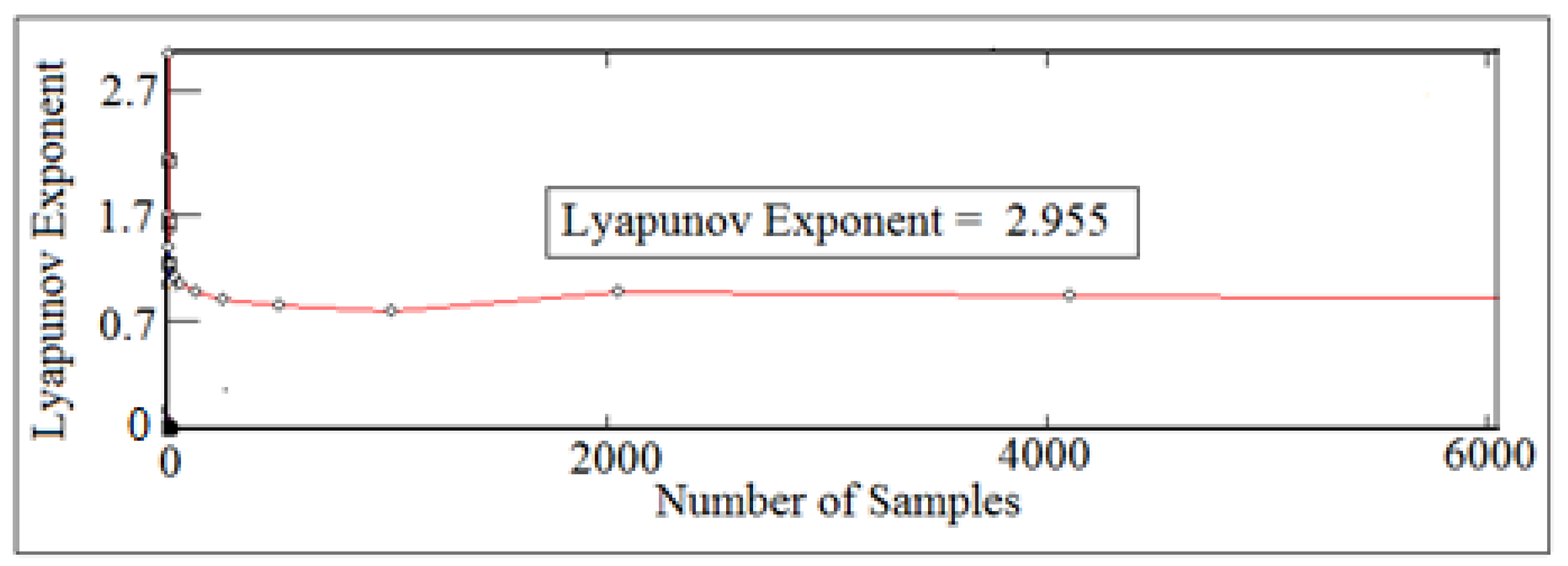
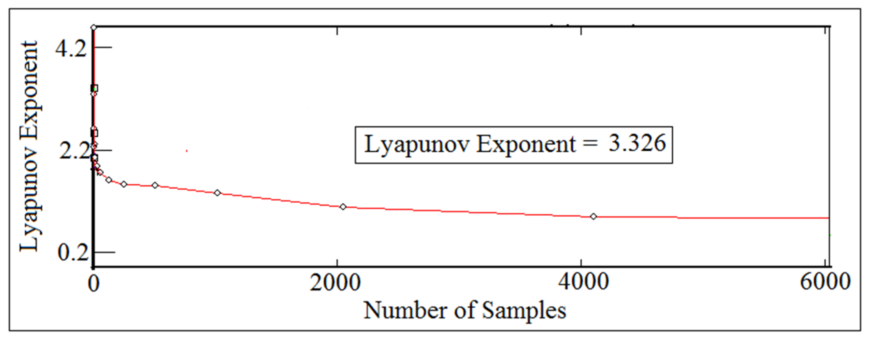
Figure 44 and Figure 45 showed the local Lyapunov exponent against number of samples at (I.D. = 17 mm and 18 mm) and (N = 600 rpm and 800 rpm), respectively. The values of Lyapunov exponent parameter were taken at their respective equilibrium point. The values of largest Lyapunov exponent were above zero and were positive, which gives indication that there will be a detachment between the cam and the follower. The detachment height of the system in Figure 45 was bigger than the detachment height of the system in Figure 44 because the system in Figure 45 has a larger value of local Lyapunov exponent than the system in Figure 44.
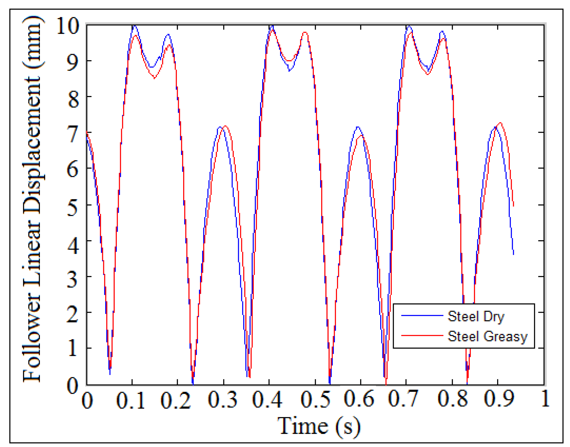
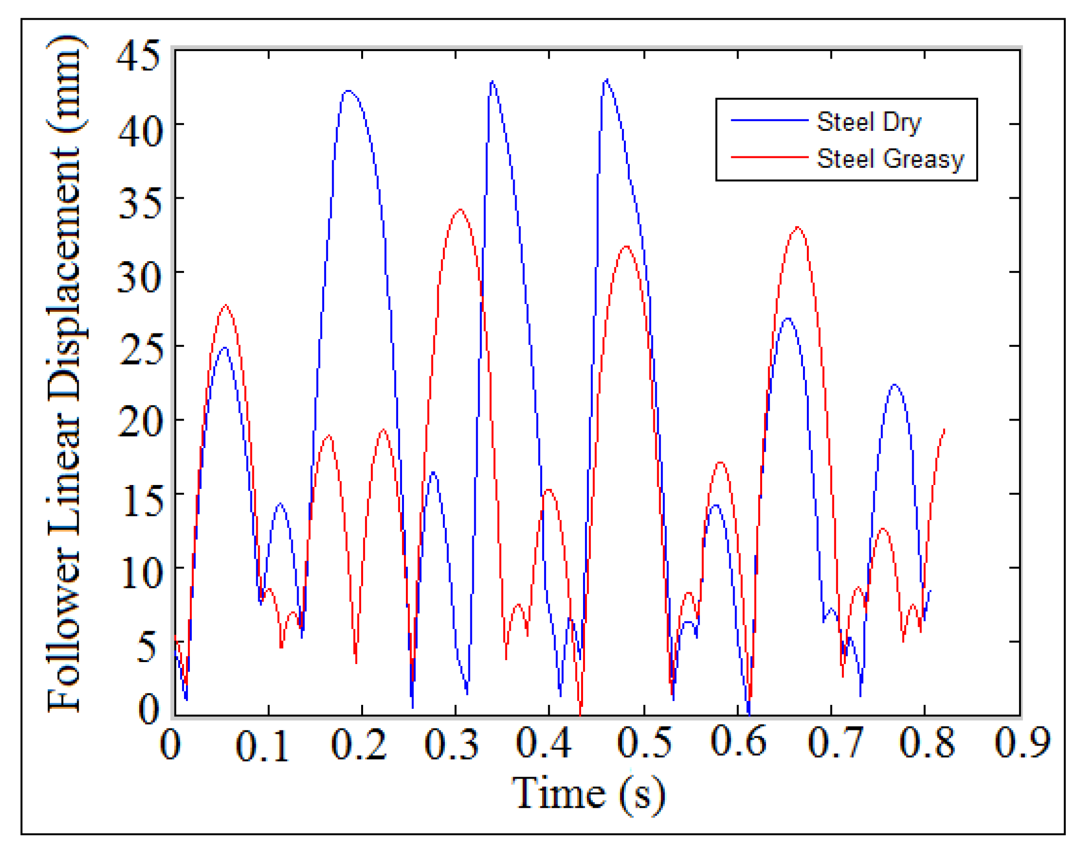
Figure 46 and Figure 47 showed the follower linear displacement against time at (I.D. = 19 mm) and (N = 200 rpm and 1000 rpm), respectively. In this comparison, two types of contacts were used, such as steel greasy and steel dry, in which the cam and the follower were made from steel. The follower displacement for the both cases were compatible, which means that there was no detachment between the cam and the follower. The steel dry and steel greasy types of the contact had no effect on the detachment heights between the cam and the follower at low speeds of the cam, as indicated in Figure 46. There was a detachment between the cam and the follower during the use of steel dry at high speeds of the cam, as shown in Figure 47. SolidWorks program was used in the contact comparison of the follower displacement using steel greasy and steel dry.
9. Conclusions
This study analyzed and discussed the detachment heights in cam follower system at different internal distance of the follower guide from inside (I.D.) and cam speeds (N). The steel dry and steel greasy types of the contact had no effect on the detachment heights between the cam and the follower at low speeds while there was a detachment between the cam and the follower during the use of steel dry at high speeds. The values of largest Lyapunov exponent were above zero and were positive, which gives indication that there will be a detachment between the cam and the follower. The peak of the follower displacement decreased with the increasing of coefficients of restitution because the potential energy of the follower has declined and dissipated due to the impact. The detachment between the cam and the follower increased with the increasing of coefficient of restitution. It can be concluded from the (FFT) diagram that there was a detachment between the cam and the follower when the contact force is approaching zero. When the black dots started disappearing from Poincare’ maps, it means that the follower was detached from the cam profile and started multi-impacts inside one cycle of the cam rotation.
Funding
This research received no external funding.
Institutional Review Board Statement
Not applicable.
Informed Consent Statement
Not applicable.
Data Availability Statement
The data that support the findings of this study are available from the corresponding author upon reasonable request.
Conflicts of Interest
The author declares that he has no conflict of interest and there is no institution was funding and supporting this research.
Article Highlights
- The detachment between the cam and the follower was detected using largest Lyapunov exponent parameter, power density function using (FFT), and Poincare’ maps due to the nonlinear dynamics phenomenon of the follower.
- Multi-degrees of freedom (spring-damper-mass) systems at the very end of the follower were used to improve the dynamic performance and to reduce the detachment height between the cam and the follower.
- Friction and impact were considered between the cam and the follower and between the follower and its guides.
- The experiment test was carried out using high speed camera at the foreground of the OPTOTRAK 30/20 equipment, while the numerical simulation was done using SolidWorks program.
Nomenclatures
| Normal Letters | |
| I.D. | Internal distance of the follower guide from inside, mm. |
| N | Cam speed, rpm. |
| I | Polar moment of inertia, . |
| Dimensions of the follower stem, mm. | |
| Spring stiffness, N/mm. | |
| Damping coefficient, Ns/mm. | |
| Spring stiffness of the three degrees of freedom, N/mm. | |
| Damping coefficient of the three degrees of freedom, Ns/mm. | |
| Radius of the base circle of the cam, mm. | |
| m | Mass of the follower, kg. |
| PC | Contact force between the cam and the follower, N. |
| d(t) | Rate of change in the distance between nearest neighbors. |
| dj(i) | Distance between the jth pair at (i) nearest neighbors, mm. |
| t | Single time series, s. |
| y(i) | Curve fitting of least square method for the follower displacement data. |
| FFT | Fast Fourier Transform of the power density function. |
| LLE | Largest Lyapunov exponent parameter. |
| Greek Letters | |
| θ | Rotational angle of the follower, Degree. |
| Ø | Phase shift angle of the vibration mode shape, Degree. |
| Pressure angle, degree. | |
| λ | Lyapunov exponent. |
| Critical speed of the cam, rpm. | |
| Latin Letters | |
| Eigenvalue problem, rpm. | |
| Discrete time steps, s. | |
| Preload extension, mm. | |
| D | Average displacement between trajectories at (t = 0). |
| Horizontal movement of the follower in the x-direction, mm. | |
| Vertical movement of the follower in the y-direction, mm. | |
| X | Equivalent solution of the follower movement, mm. |
| , | Velocity, and acceleration of the roller follower, mm/s, mm/s2. |
Appendix A
The cam follower mechanism can be treated as a single or multi-degrees of freedom based on the motion of the follower. By applying the Newton’s second law of translation motion in the y-direction, it can be obtained:
After simplification Equation (A1):
By applying the Newton’s second law of translation motion in the x-direction on the follower stem, it can be obtained:
After simplification Equation (A3):
By applying Newton’s second law of rotation motion about the point in the middle of the follower stem:
After simplification Equation (A5):
where:
Put the equations of motion Equations (A2), (A4) and (A6) in matrix form:
where:
Equation (A7) can now be put into terms of frequency response matrix which is also called the impedance matrix as follows:
where:
The Eigenvalue problem is solved when the determinant of the impedance matrix equal to zero.
The amplitude of Eigenvectors problem (mode shape) is calculated by taking the inverse of the impedance matrix and multiplying by the force vector.
The solution of the multi-body dynamics response is as in below:
The contact force between the cam and the follower is illustrated in the following equation:
where:
The analytic solution of the follower displacement is as in below because the follower displacement is varied in x and y directions:
Appendix B
The numerical simulation of SolidWorks program were illustrated in the following steps as in below:
- (a)
- Ten parts such as (polydynecam.SLDPRT, flat-facedfollower.SLDPRT,guideno1.SLDPRT, guideno2.SLDPRT, outsideframe.SLDPRT, massboxno1.SLDPRT, massboxno2.SLDPRT, massboxno3.SLDPRT, massboxno4.SLDPRT, and cylindricalrollers.SLDPRT) has been created using the modeling computer aided design (CAD) of SolidWorks program. It can be assembled the above nine parts using camfollowerassembly.SLDASM to obtain Figure 5.
- (b)
- Select Motion Analysis from Motion Study Tab and select number frames per second equal to 1000 to make the solution of the dynamic motion more accurate.
- (c)
- Select the Option of Units from Document Properties Tab and select MMGS.
- (d)
- Select Gravity from Motion Study Tab and select the y-direction.
- (e)
- Select Contact from Motion Study Tab and check mark the box of Use Contact Groups in which there will be two boxes. Select the cam geometry in the first box and select the follower geometry in the second box to make the contact between the cam and the follower. Also there will be another two boxes to make the contact between the follower and the two guides.
- (f)
- Select Motor button from Motion Study Tab and select Rotary Motor and the cam speed should be constant.
- (g)
- Select Mechanical Mate from Mate button to make the mate between the cam and the follower.
- (h)
- Select the integrator type GSTIFF from Advanced Motion Analysis Options Tab.
- (i)
- Select Force button from Motion Study Tab and enter the spring force between the follower and the installation table as an external constant force.
- (j)
- Select Spring button from Motion Study Tab to apply multi-degrees of freedom (spring-damper-mass system) and enter the spring constant and the damping coefficient and select the top and bottom surfaces of mass box no. 2, 3, and 4. To apply the spring and damper on mass box no. 1 select the bottom surface of the outside frame and top surface of mass box no. 1. Moreover, to apply the spring and damper on mass box no. 4 select the bottom surface of mass box no. 4 and the very end top of follower stem.
- (k)
- Select Calculate from the Motion Study Tab to solve for the motion study.
- (l)
- Select Results button from Motion Study Table Select Displacement and Linear Displacement to obtain the follower displacement against time and select lower surface of guide no.2 and the contact point between the cam and the follower. On the other hand, select from Results button Forces and select Contact Force and select lower surface of guide no.2 and select the contact point between the cam and the follower to obtain the contact force against time.
References
- Sundar, S.; Dreyer, J.T.; Singh, R. Rotational sliding contact dynamics in a non-linear cam-follower system as excited by a periodic motion. J. Vib. Acoust. 2013, 332, 4280–4295. [Google Scholar] [CrossRef]
- Yan, H.S.; Tsay, W.J. A variable-speed approach for preventing cam-follower separation. J. Adv. Mech. Des. Syst. Manuf. 2008, 2, 12–23. [Google Scholar] [CrossRef] [Green Version]
- Jamali, U.H.; Al-Hamood, A.; Abdulla, O.I.; Senatore, I.; Schlattmann, J. Lubrication analyses of cam and flat-faced follower. Lubricants 2019, 7, 31. [Google Scholar] [CrossRef] [Green Version]
- Pugliese, G.; Ciulli, E.; Fazzolari, F. Experimental aspects of a cam-follower contact. In IFToMM World Congress on Mechanism and Machine Science; Springer: Berlin/Heidelberg, Germany, 2019; pp. 3815–3824. [Google Scholar]
- Ciulli, E.; Fazzolari, F.; Pugliese, G. Contact Force Measurements in Cam and Follower Lubricated Contacts. Front. J. Front. Mech. Eng. 2020, 6, 601410. [Google Scholar] [CrossRef]
- Alzate, R.; Di Bernardo, M.; Montanaro, U.; Santini, S. Experimental and numerical verification of bifurcations and chaos in cam-follower impacting systems. J. Nonlinear Dyn. 2007, 50, 409–429. [Google Scholar] [CrossRef] [Green Version]
- Desai, H.D.; Patel, V.K. Computer aided kinematic and dynamicanalysis of cam and follower. In Proceedings of the World Congress on Engineering WCE 2010, London, UK, 30 June–2 July 2010; Volume II. [Google Scholar]
- Yang, Y.-F.; Lu, Y.; Jiang, T.-D.; Lu, N. Modeling and nonlinear response of the cam-follower oblique-impact system. Disc. Dyn. Nat. Soc. 2016, 2016, 1–8. [Google Scholar] [CrossRef] [Green Version]
- Lassaad, W.; Mohamed, T.; Yassine, D.; Fakher, C.; Taher, F.; Mohamed, H. Nonlinear dynamic behavior of a cam mechanism with oscillating roller follower in presence of profile error. Front. J. Front. Mech. Eng. 2013, 8, 127–136. [Google Scholar] [CrossRef]
- DasGupta, A.; Ghosh, A. On the determination of basic dimensions of a cam with a translating roller-follower. J. Mech. Des. 2004, 126, 143–147. [Google Scholar] [CrossRef]
- Yousuf, L.S.; Marghitu, B.D. Nonlinear dynamics behavior of cam-follower system using concave curvatures profile. Adv. Mech. Eng. 2020, 12, 1687814020945920. [Google Scholar] [CrossRef]
- Belliveau, K.D. An Investigation of Incipient Jump in Industrial Cam Follower Systems. Master’s Thesis, Worcester Polytechnic Institute, Worcester, MA, USA, 2002. [Google Scholar]
- Hejma, P.; Svoboda, M.; Kampo, J.; Soukup, J. Analytic analysis of a cam mechanism. Procedia Eng. 2017, 177, 3–10. [Google Scholar] [CrossRef]
- Yousuf, L.S. Non-periodic motion reduction in globoidal cam with roller follower mechanism. Proc. Inst. Mech. Eng. C J. Mech. Eng. Sci. 2021, 09544062211033642. [Google Scholar] [CrossRef]
- Sinha, A.; Bharti, K.S.; Samantaray, A.K.; Bhattacharyya, R. Sommerfeld effect in a single-DOF system with base excitation from motor driven mechanism. Mech. Mach. Theory 2020, 148, 103808. [Google Scholar] [CrossRef]
- Yousuf, L.S. Investigation of chaos in a polydyne cam with flat-faced follower mechanism. J. King Saud Univ. Eng. Sci. 2021, 33, 507–516. [Google Scholar] [CrossRef]
- Norton, R.L. Cam Design and Manufacturing Handbook; Industrial Press: New York, NY, USA, 2002. [Google Scholar]
- Sinha, A. Vibration of Mechanical Systems, 1st ed.; Cambridge University Press: Cambridge, UK, 2010. [Google Scholar]
- Shakoor, M.M. Fatigue Life Investigation for Cams with Translating Roller-Follower and Translating Flat-Face Follower Systems. Ph.D. Thesis, Iowa State University, Ames, IA, USA, 2006. [Google Scholar]
- Hamza, F.; Abderazek, H.; Lakhdar, S.; Ferhat, D.; Yıldız, A.R. Optimum design of cam-roller follower mechanism using a new evolutionary algorithm. Int. J. Adv. Manuf. Syst. 2018, 99, 1267–1282. [Google Scholar] [CrossRef]
- Planchard, D. SolidWorks 2016 Reference Guide: A Comprehensive Reference Guide with over 250 Standalone Tutorials; Sdc: Kansas, KS, USA, 2015. [Google Scholar]
- Yousuf, L.S.; Marghitu, D.B. Experimental and Simulation of a Cam and Translated Roller Follower Over a Range of Speeds. In ASME International Mechanical Engineering Congress and Exposition; ASME: New York, NY, USA, 2016; p. V04AT05A057. [Google Scholar]
- Rothbart, H.A. Cam Design Handbook; McGraw-Hill Education: New York, NY, USA, 2004. [Google Scholar]
- Nguyen, T.T.N.; Hüsing, M.; Corves, B. Motion Design of Cam Mechanisms by Using Non-Uniform Rational B-Spline. Ph.D. Thesis, Rheinisch-Westfälischen Aachen University of Technology, Aachen, Germany, 2018. [Google Scholar]
- Wu, L.I.; Liu, C.H.; Chen, T.W. Disc cam mechanisms with concave-face follower. Proc. Inst. Mech. Eng. C J. Mech. Eng. Sci. 2009, 223, 1443–1448. [Google Scholar] [CrossRef]
- Parlitz, U. Estimating Lyapunov Exponents from Time Series. Chaos Detection and Predictability; Springer: Berlin/Heidelberg, Germany, 2016; pp. 1–34. [Google Scholar]
- Terrier, P.; Fabienne, R. Maximum Lyapunov exponent revisited: Long-term attractor divergence of gait dynamics is highly sensitive to the noise structure of stride intervals. Gait Posture 2018, 66, 236–241. [Google Scholar] [CrossRef] [PubMed] [Green Version]
- Hussain, V.S.; Spano, M.L.; Lockhart, T.E. Effect of data length on time delay and embedding dimension for calculating the Lyapunov exponent in walking. J. R. Soc. Interface 2020, 17, 20200311. [Google Scholar] [CrossRef] [PubMed]
- Garcia, M.M.; Morales, I.; Rodriguez, J.M.; Marin, M.R. Selection of embedding dimension and delay time in phase space reconstruction via symbolic dynamics. J. Entropy 2021, 23, 221. [Google Scholar] [CrossRef] [PubMed]
- Stoica, P.; Moses, R.L. Spectral Analysis of Signals; Pearson Prentice Hall Upper Saddle River: Upper Saddle River, NJ, USA, 2005. [Google Scholar]
- Abu-Mahfouz, I. Experimental investigation of non-linear behavior of a cam-follower mechanism. In SEM Annual Conference and Exposition on Experimental and Applied Mechanics; Elsevier: Springfield, MA, USA, 2005. [Google Scholar]
Figure 1.
Experiment setup of cam–follower mechanism.

Figure 2.
Applied load against spring deflection.

Figure 3.
Cam speed against weight.

Figure 4.
Three degrees of freedom of flat-faced follower.

Figure 5.
Computer aided design of SolidWorks simulation using multi-degrees of freedom.

Figure 6.
Follower linear displacement against time using multi-degrees of freedom systems.

Figure 7.
Nonlinear response of the follower displacement in the x and y directions.

Figure 8.
Follower linear displacement mapping against time for (I.D. = 16 mm).

Figure 9.
Follower linear displacement mapping against time for (I.D. = 17 mm).

Figure 10.
(a) Impact between the follower and the guide. (b) Diagram shows the follower stem with the guide.
Figure 10.
(a) Impact between the follower and the guide. (b) Diagram shows the follower stem with the guide.

Figure 11.
Follower linear displacement mapping against time at different values of coefficient of restitution.
Figure 11.
Follower linear displacement mapping against time at different values of coefficient of restitution.

Figure 12.
Comparison of follower linear displacement.

Figure 13.
Comparison of nonlinear response of the follower.

Figure 14.
Contact force mapping against time at different cam speeds for (I.D. = 16 mm).

Figure 15.
Contact force mapping against time at different cam speeds for (I.D. = 17 mm).

Figure 16.
Comparison of contact force against time.

Figure 17.
Experiment simulation of internal distance of the follower guide with clearance.

Figure 18.
Local Lyapunov exponent against number of samples for (I.D. = 16 mm) and (N = 400 rpm).

Figure 19.
Time delay of numerical simulation.

Figure 20.
Time delay of experiment test.

Figure 21.
Embedding dimensions of numerical simulation.

Figure 22.
Embedding dimensions of experiment test.

Figure 23.
Average logarithmic divergence against the time for (I.D. = 16 mm) and (N = 200 rpm).

Figure 24.
Power density function of the experiment test.

Figure 25.
Power density function of the numerical simulation.

Figure 26.
Poincare’ maps for (I.D. = 16 mm) at different cam speeds.

Figure 27.
Poincare’ maps for (I.D. = 18 mm) at different cam speeds.

Figure 28.
Phase-plane diagram mapping using different values of coefficient of restitution.

Figure 29.
Follower linear displacement mapping against time for (I.D. = 18 mm).

Figure 30.
Follower linear displacement mapping against time for (I.D. = 19 mm).

Figure 31.
Contact force mapping against time for (I.D. = 18 mm).

Figure 32.
Contact force mapping against time for (I.D. = 19 mm).

Figure 33.
Maximum follower detachment heights against cam speeds.

Figure 34.
Power density function of the experiment test.

Figure 35.
Power density function of the numerical simulation.

Figure 36.
Largest Lyapunov exponent against cam speeds.

Figure 37.
Follower linear displacement against time at different values of coefficient of restitution.
Figure 37.
Follower linear displacement against time at different values of coefficient of restitution.

Figure 38.
Comparison of follower linear displacement against time.

Figure 39.
Comparison of follower linear velocity against time.

Figure 40.
Comparison of follower linear acceleration against time.

Figure 41.
Poincare’ maps for (I.D. = 17 mm) at different cam speeds.

Figure 42.
Poincare’ maps for (I.D. = 19 mm) at different cam speeds.

Figure 43.
Average logarithmic divergence against the time for (I.D. = 18 mm) and (N = 200 rpm).

Figure 44.
Local Lyapunov exponent against number of samples for (I.D. = 17 mm) and (N = 600 rpm).

Figure 45.
Local Lyapunov exponent against number of samples for (I.D. = 18 mm) and (N = 800 rpm).

Figure 46.
Follower linear displacement against time at (I.D. = 19 mm) and (N = 200 rpm) using different types of contacts.
Figure 46.
Follower linear displacement against time at (I.D. = 19 mm) and (N = 200 rpm) using different types of contacts.

Figure 47.
Follower linear displacement against time at (I.D. = 19 mm) and (N = 1000 rpm) using different types of contacts.
Figure 47.
Follower linear displacement against time at (I.D. = 19 mm) and (N = 1000 rpm) using different types of contacts.

Publisher’s Note: MDPI stays neutral with regard to jurisdictional claims in published maps and institutional affiliations. |
© 2021 by the author. Licensee MDPI, Basel, Switzerland. This article is an open access article distributed under the terms and conditions of the Creative Commons Attribution (CC BY) license (https://creativecommons.org/licenses/by/4.0/).
Share and Cite
MDPI and ACS Style
Yousuf, L.S. Detachment Detection in Cam Follower System Due to Nonlinear Dynamics Phenomenon. Machines 2021, 9, 349. https://doi.org/10.3390/machines9120349
AMA Style
Yousuf LS. Detachment Detection in Cam Follower System Due to Nonlinear Dynamics Phenomenon. Machines. 2021; 9(12):349. https://doi.org/10.3390/machines9120349
Chicago/Turabian StyleYousuf, Louay S. 2021. "Detachment Detection in Cam Follower System Due to Nonlinear Dynamics Phenomenon" Machines 9, no. 12: 349. https://doi.org/10.3390/machines9120349
Note that from the first issue of 2016, this journal uses article numbers instead of page numbers. See further details here.