
Machinery Foundations Dynamical Analysis: A Case Study on Reciprocating Compressor Foundation


 ,
, 
Abstract
:1. Introduction
- Section 2: Materials and methods, Barkan’s rigid body analytical calculation, FEM and dynamic soil analysis;
- Section 3: Case study, the considered geometry and inputs are described;
- Section 4: Results and discussion, the original geometry of the foundation is reduced and the results of the different analyses are discussed;
- Section 5: Conclusion, the main results are summarized, and future developments of the topic are introduced.
2. Materials and Methods
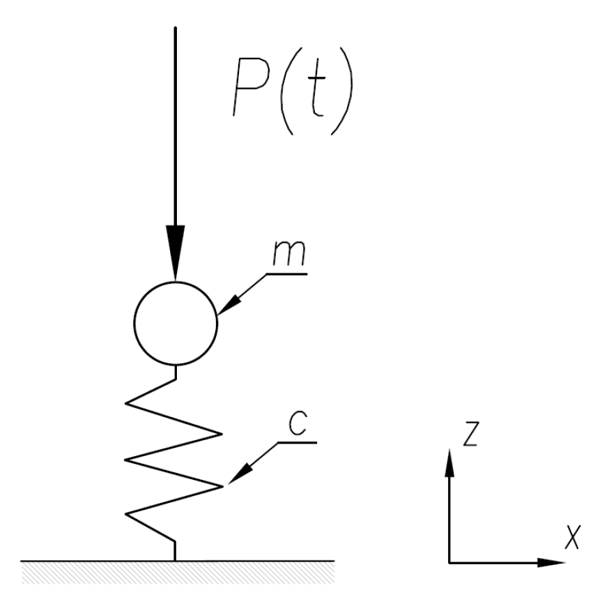
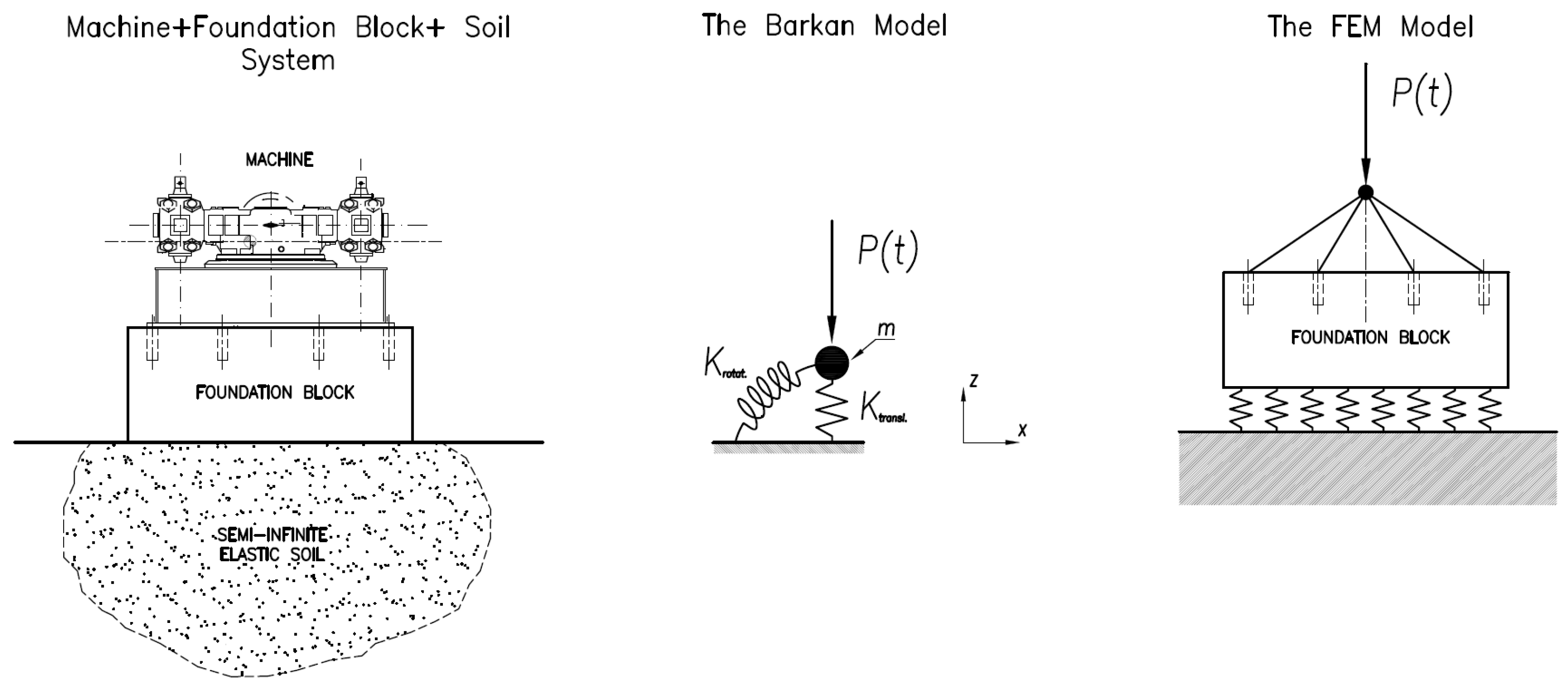
2.1. Barkan’s Rigid Body Analytical Calculation Method
- -
- the foundation block is considered a rigid body;
- -
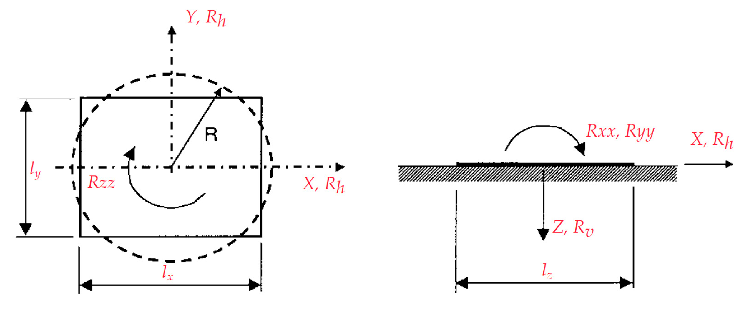
- the soil is modelled as a spring and can be summarized with a rotational and translational degree of freedom referred to as an orthonormal reference system jointed to the body;
- -
- under dynamical loads, there is a linear relationship between foundation block displacement and soil reaction and between vibration amplitude and exciting force. The soil is assumed as a bed of springs with stiffness expressed by the elastic coefficients of compression and shear;
- -
- the vibrational response of the system composed of the machine, foundation and soil under the dynamical load is in frequency with the load applied;
- -
- the dynamical soil response is assumed to be a mass-spring viscous damper system;
- -
- the soil under the foundation has no inertial properties but only elastic properties.
- G′ dynamic shear modulus;
- µ Poisson modulus;
- L, B the semi-length and the semi-width of the base rectangle of foundation;
- D embedment depth;
- d height of foundation lateral surface in contact with the soil (d ≤ D);
- Aw area of foundation lateral surface in contact with the soil;
- Ab area of the rectangular surface of the foundation base in contact with soil;
- dimensionless parameters depending to the soil typology
- static stiffness values;
- ki stiffness coefficients for the calculation of dynamic stiffness values; they are a function of L, B, D, , where the- dimensionless amplitude is expressed by means ratiowhere Vs shear waves speed in the ground.
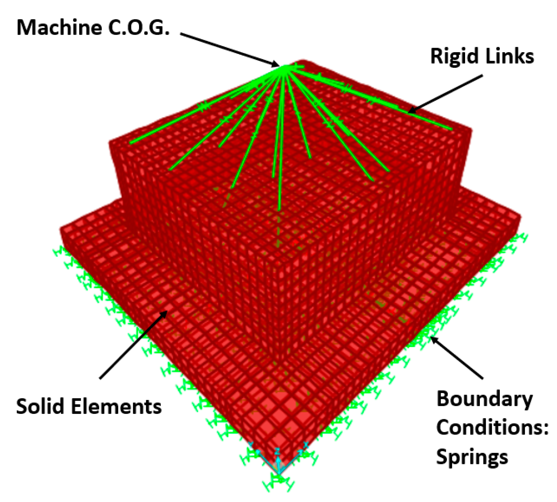
2.2. Finite Element Method
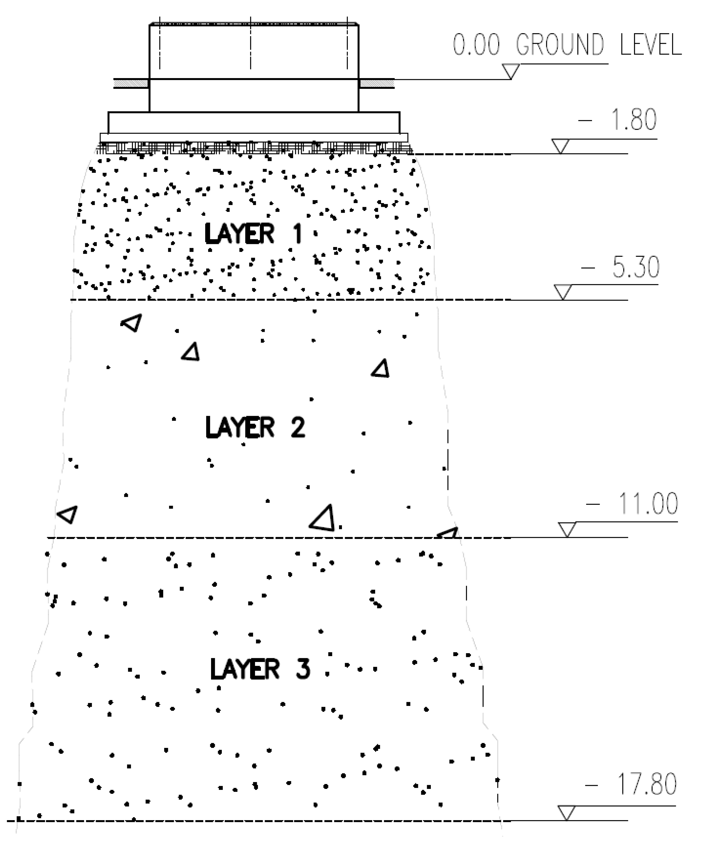
2.3. The Soil Model and the Dynamical Analysis
- is soil density;
- G’ is the dynamic shear module;
- ω is the pulsation of excitement;
- can be used for rectangular bases with the following expression:the key value to identify the frequency is the through the pulsation and the dimension B of the circular base; is the velocity of the propagation of the waves, which is directly linked to the shear module G.
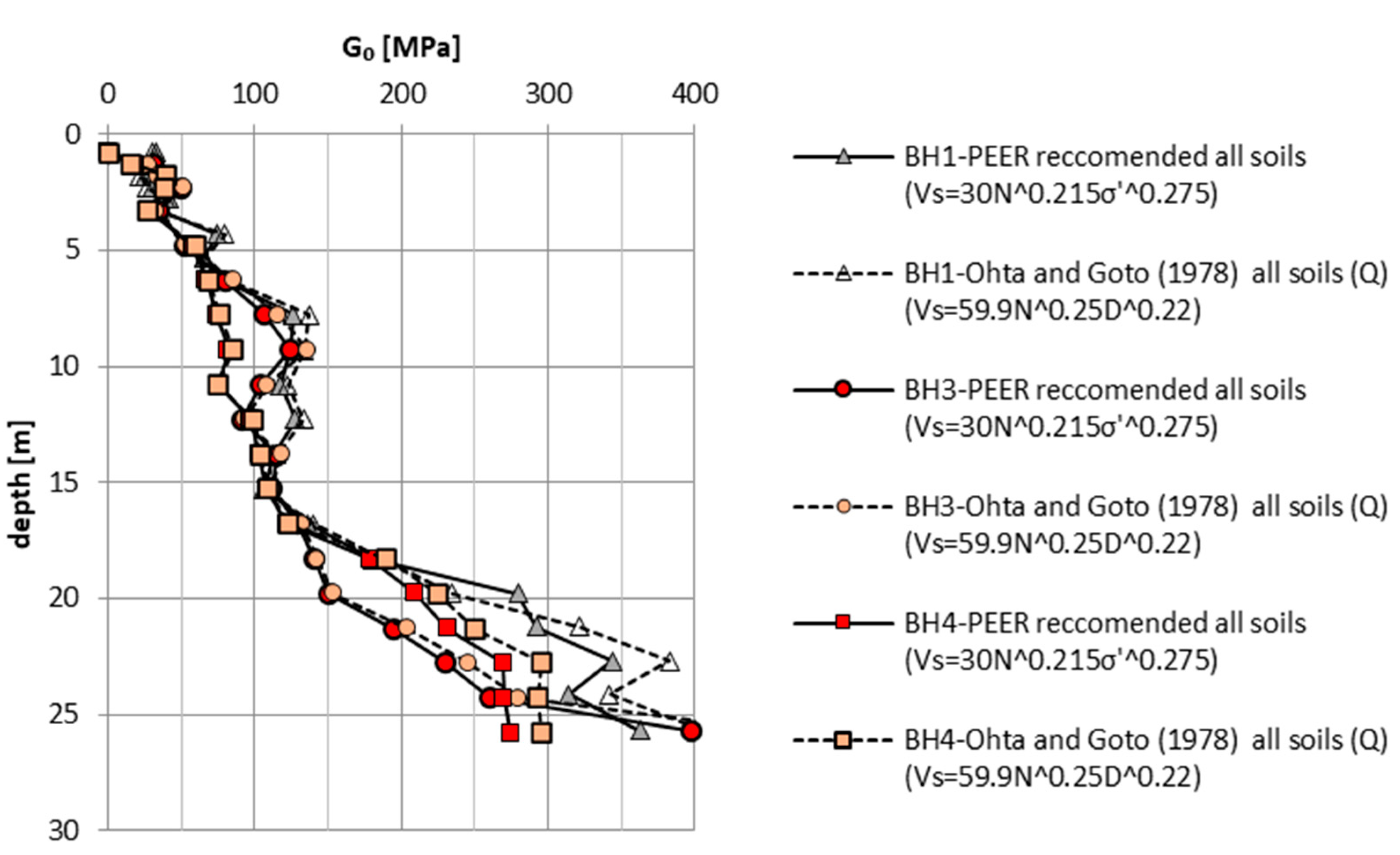
- = numeric coefficient;
- = SPT N-value is a uniform reference energy ratio of 60% of the theoretical SPT energy (N60);
- Q = quaternary age;
- is the total and effective stress.
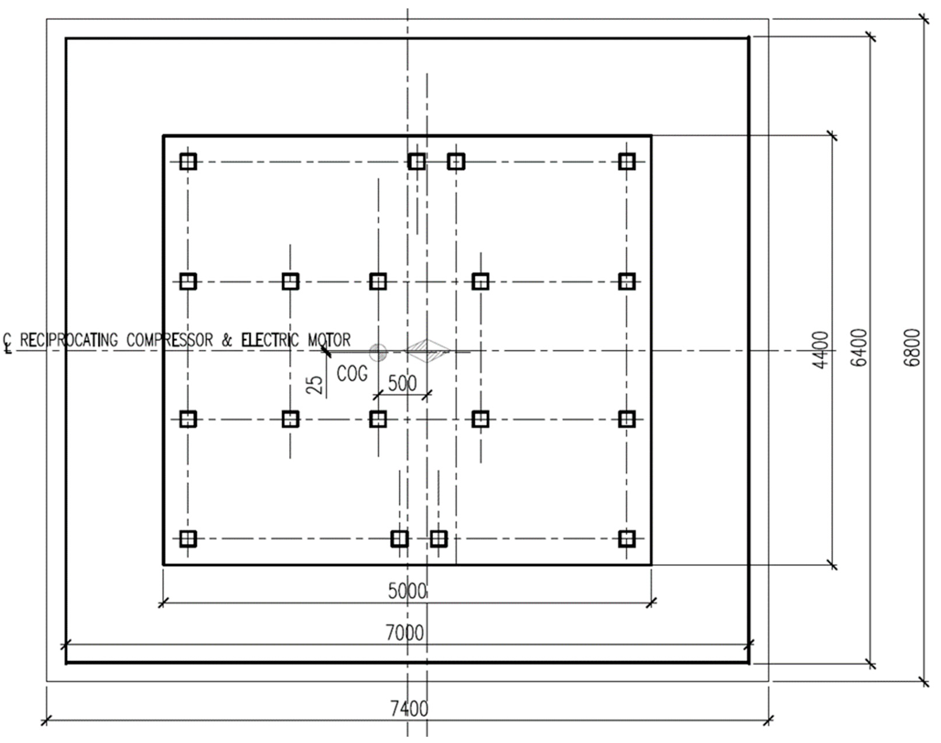
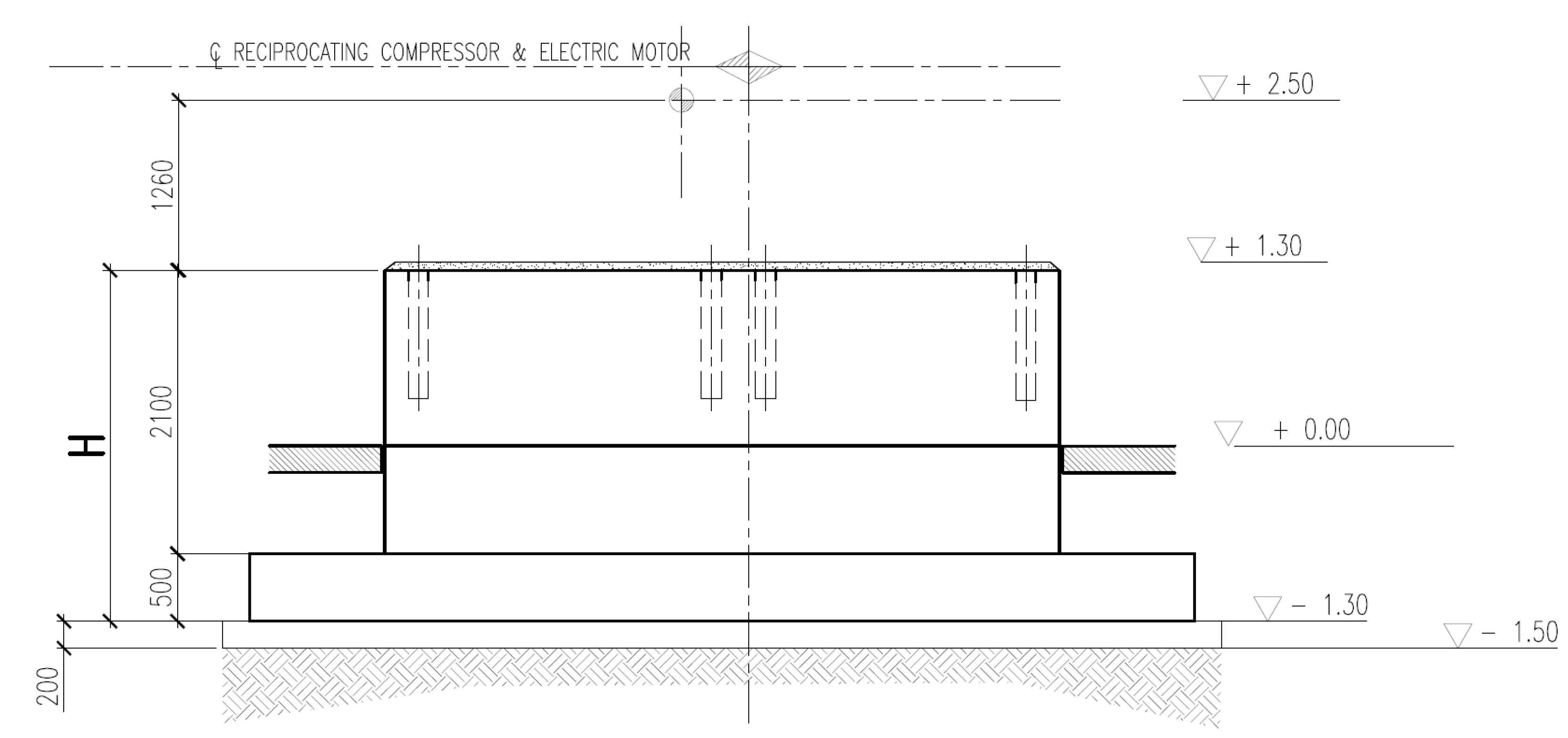
3. Case Study on Reciprocating Compressor Foundations
4. Results and Discussion
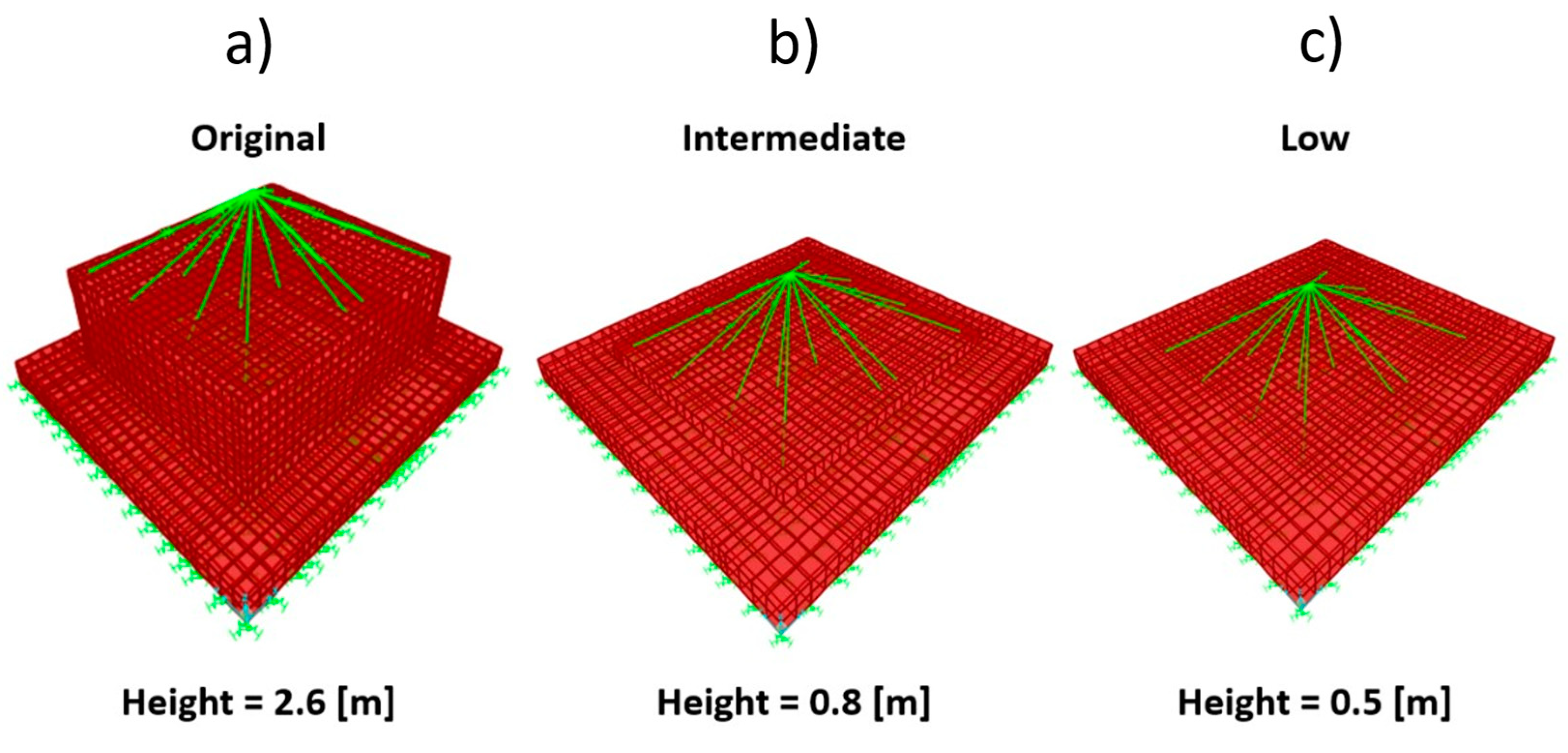
4.1. 1st Model—Original Height
- -
- Translational vertical stiffness, Kv, 3467.62 [MN/m]
- -
- Translational horizontal stiffness, Kh, 3379.93 [MN/m]
- -
- Rotational stiffness about x-axis, Kxx, 45,378.46 [MNm/rad]
- -
- Rotational stiffness about y-axis, Kyy, 51,365.58 [MNm/rad]
- -
- Rotational stiffness about z-axis, Kzz, 78,317.45 [MNm/rad]
4.2. 2nd Model—Intermediate Height
- -
- Translational vertical stiffness, Kv, 3277.93 [MN/m]
- -
- Translational horizontal stiffness, Kh, 3205.79 [MN/m]
- -
- Rotational stiffness about x-axis, Kxx, 44,023.98 [MNm/rad]
- -
- Rotational stiffness about y-axis, Kyy, 49,788.52 [MNm/rad]
- -
- Rotational stiffness about z-axis, Kzz, 78,317.45 [MNm/rad]
4.3. 3rd Model—Low Height
- -
- Translational vertical stiffness, Kv, 3159.59 [MN/m]
- -
- Translational horizontal stiffness, Kh, 3078.89 [MN/m]
- -
- Rotational stiffness about x-axis, Kxx, 442,860.12 [MNm/rad]
- -
- Rotational stiffness about y-axis, Kyy, 48,440.19 [MNm/rad]
- -
- Rotational stiffness about z-axis, Kzz, 78,317.45 [MNm/rad]
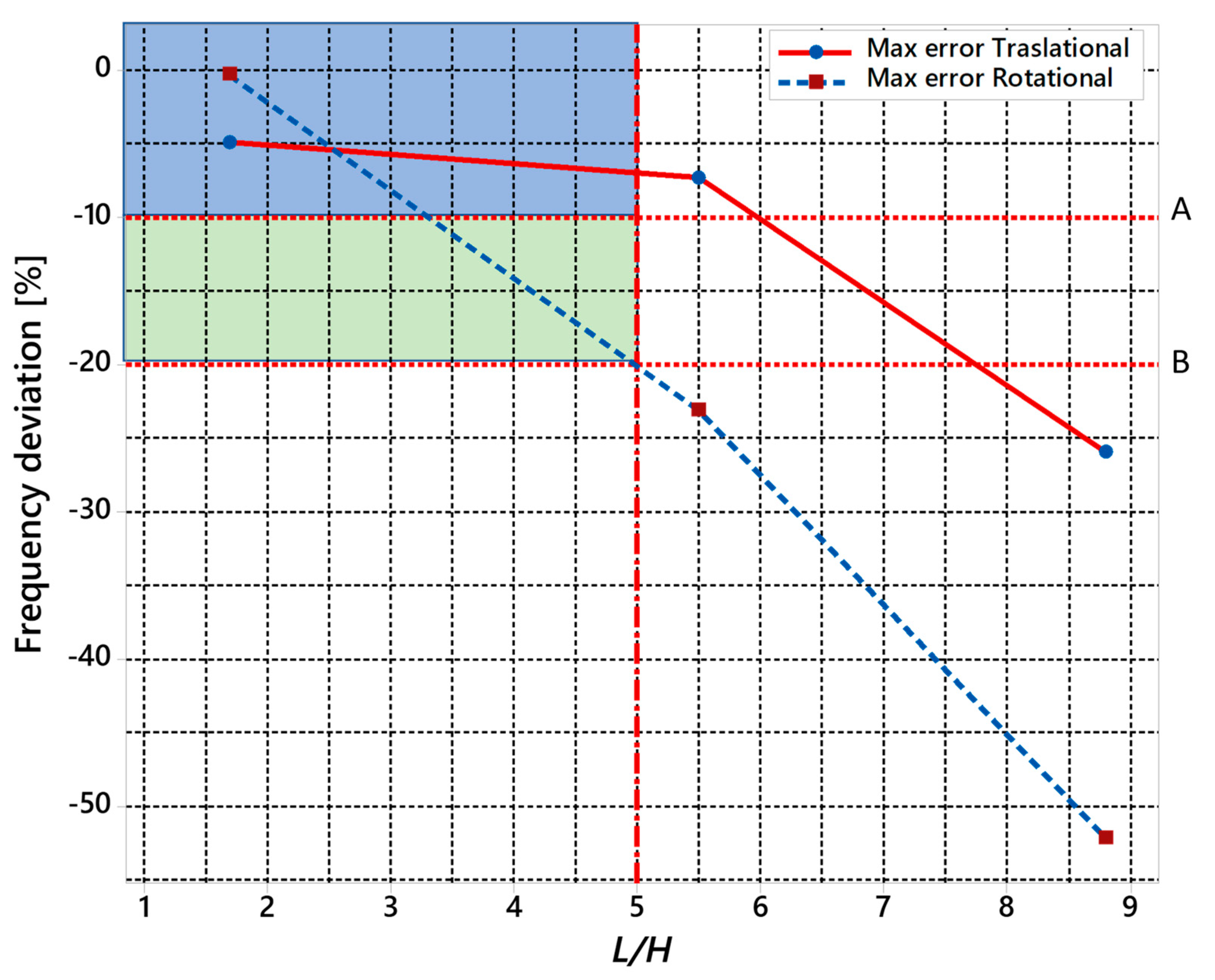
4.4. Discussion
5. Conclusions
- -
- evaluate the response of the system resting on an elastic soil model as per the Winkler bed model, obtaining different responses to compare;
- -
- calculate the amplification factor based on FEA and Barkan analysis and identify the displacement of the system comparing with the specification limits;
- -
- identify the difference between results from FEA and Barkan analysis, changing geometries;
- -
- model the soil, differentiating for each stratum different bed springs and analyzing the dynamical response with FEM;
- -
- model the machine and soil with stiffeners and differentiating for each stratum different bed spring, and analyzing the dynamical response with FEM;
- -
- model each component of the machine with appropriate stiffeners, analyze the model of the system machine, foundation and soil, calculating the response;
- -
- model the soil with a nonlinear spring and calculate the dynamical response to further develop the topics covered.
Author Contributions
Funding
Conflicts of Interest
References
- ASME. Process Piping; ASME: New York, NY, USA, 2020. [Google Scholar]
- Ziolkowski, P.; Demczynski, S.; Niedostatkiewicz, M. Assessment of Failure Occurrence Rate for Concrete Machine Foundations Used in Gas and Oil Industry by Machine Learning. Appl. Sci. 2019, 9, 3267. [Google Scholar] [CrossRef] [Green Version]
- Ciappi, A.; Giorgetti, A.; Ceccanti, F.; Canegallo, G. Technological and economical consideration for turbine blade tip restoration through metal deposition technologies. Proc. Inst. Mech. Eng. Part C J. Mech. Eng. Sci. 2021, 235, 1741–1758. [Google Scholar] [CrossRef]
- Barkan, D.D. Dynamics of Bases and Foundations; McGraw Hill Book: New York, NY, USA, 1962. [Google Scholar]
- Bowles, J.E. Foundation Analysis and Design, 5th ed.; McGraw-Hill, Inc.: Singapore, 1997. [Google Scholar]
- Arya, S.C.; O’Neil, M.W.; Pincus, G. Design of Structures and Foundations for Vibrating Machines; Gulf Publishing Company Book Division: Houston, TX, USA, 1984. [Google Scholar]
- Novak, M.; Aboul-Ella, F. Impedance Functions of Piles in Layered Media. J. Eng. Mech. Div. 1978, 104, 3. [Google Scholar]
- Lamb, H. On the propagation of tremors over the surface of an elastic solid. Phil. Trans. A 1904, 203, 1–42. [Google Scholar]
- Dobry, R.; Gazetas, G. Simple method for dynamic stiffness and damping of floating pile groups. Geotechnique 1988, 38, 557–574. [Google Scholar] [CrossRef]
- Gazetas, G. Analysis of Machine Foundation Vibrations: State of Art. Soil Dyn. Earthq. Eng. 1983, 2, 2–41. [Google Scholar] [CrossRef]
- Hall, J.R.; Richart, F.E. Effect of Vibration Amplitude on Wave Velocities in Granular Materials. In Proceedings of the Second Pan American Conference on Soil Mechanics and Foundation Engineering, São Paulo, Brazil, 14–24 July 1963; Volume I. [Google Scholar]
- Drnevich, V.P.; Hall, J.R. Transient loading tests on a circular footing. J. Soil Mech. Found. 1966, 92, 153–167. [Google Scholar] [CrossRef]
- Lysmer, J.; Richart, F.E. Dynamic Response of Footings to Vertical Loading. J. Soil Mech. Found. Div. 1966, 92, 65–91. [Google Scholar] [CrossRef]
- Whitman, R.V.; Richart, F.E. Discussion of Design Procedures for Dynamically Loaded Foundations. J. Soil Mech. Found. Div. 1969, 95, 364–366. [Google Scholar] [CrossRef]
- Lysmer, J.; Kuhlemeyer, R.L. Finite Dynamic Model for Infinite Media. J. Eng. Mech. Div. 1971, 95, 859–877. [Google Scholar] [CrossRef]
- Wedpathak, A.V.; Desai, P.J.; Pandit, V.K.; Guha, S.K. Vibrations of Block Type Machine Foundations Due to Impact Loads. In Proceedings of the Fifth Symposium on Earthquake Engineering, Merut, India, 9–11 November 1974; Volume I, pp. 219–226. [Google Scholar]
- IS 2974 Code of Practice for Design and Construction of Machine Foundations, Part I: Foundation for Reciprocating Type Machines; Bureau of Indian Standards: New Delhi, India, 2008. Available online: https://law.resource.org/pub/in/bis/S03/is.2974.1.1982.pdf (accessed on 30 September 2021).
- Liu, H. Concrete Foundations for Turbine Generators: Analysis, Design, and Construction; ASCE: Reston, VA, USA, 2018. [Google Scholar]
- Wair, B.R.; DeJong, J.T.; Shantz, T. Guidelines for Estimation of Shear Wave Velocity Profiles; PEER Report 2012/08; Pacific Earthquake Engineering Research Center, Headquarters at the University of California: Berkeley, CA, USA, 2012. [Google Scholar]
- ASTM. ASTM D1586-99 Standard Test Method for Penetration Test and Split-Barrel Sampling on Soils; Annual Book of ASTM Standards, vol. 04.08; American Society of Testing and Material: West Conshohocken, PA, USA, 1999. [Google Scholar]


| Top | Bottom | Thickness | ρ | Vs | ν | G | E | |
|---|---|---|---|---|---|---|---|---|
| m | m | m | t/m3 | m/s | MPa | MPa | ||
| layer 1 | 1.80 | 5.30 | 3.50 | 2.00 | 141 | 0.49 | 40 | 119 |
| layer 2 | 5.30 | 11.00 | 5.70 | 2.00 | 224 | 0.49 | 100 | 298 |
| layer 3 | 11.00 | 17.80 | 6.80 | 2.00 | 255 | 0.49 | 130 | 387 |
| Original Height | Translation in x Direction Freq. | Translation in y Direction Freq. | Translation in z Direction Freq. | Rotation about x-Axis Freq. | Rotation about y-Axis Freq. | Rotation about z-Axis Freq. |
|---|---|---|---|---|---|---|
| Barkan’s Theory | 18.5 | 18.5 | 18.7 | 30.0 | 30.0 | 37.0 |
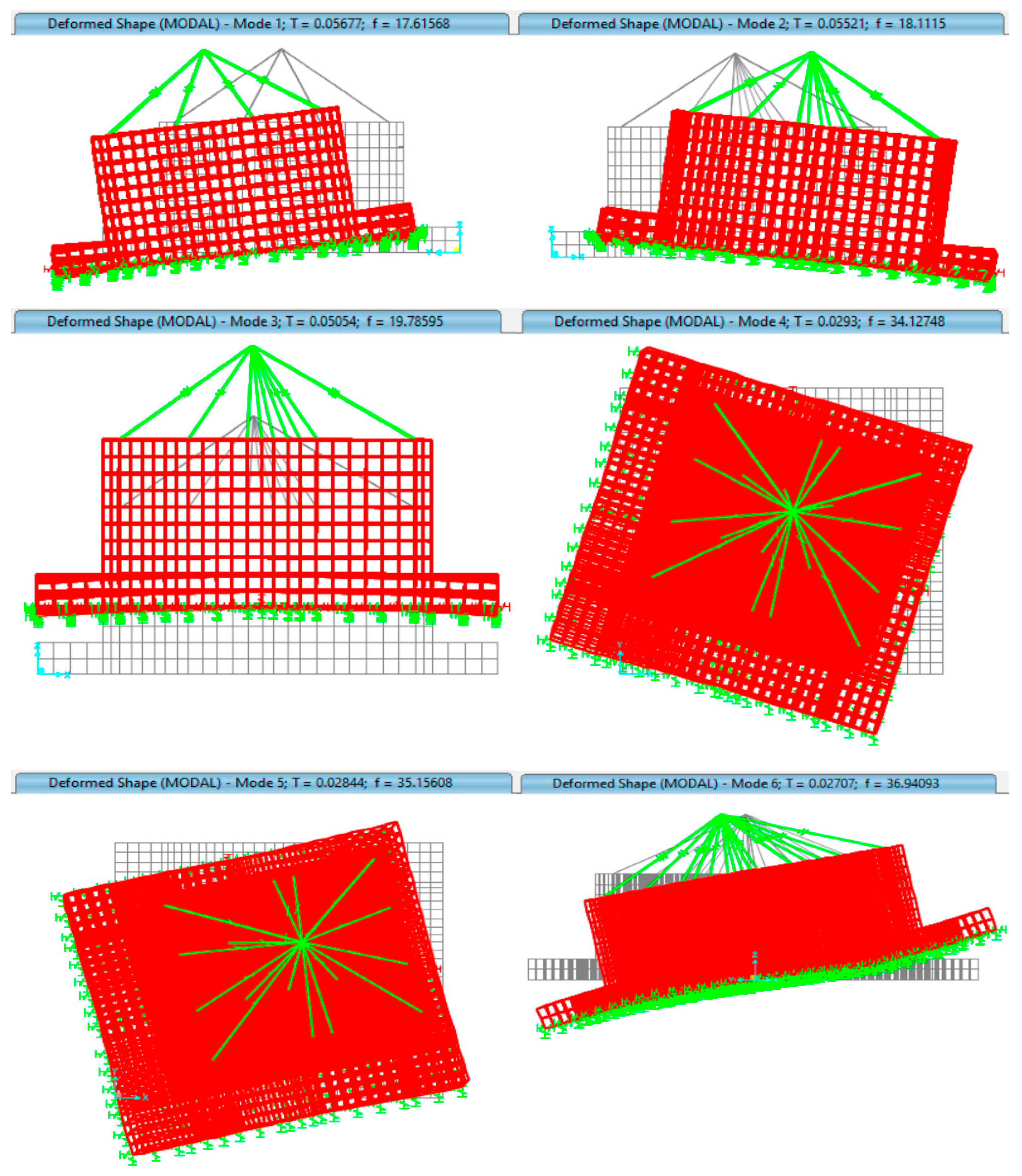
| FEA | 17.6 | 18.1 | 19.8 | 34.1 | 35.2 | 36.9 |
| Frequency deviation [%] | −4.9 | −2.2 | 5.9 | 13.7 | 17.3 | −0.3 |
| Original Height | Translation in x Direction Freq. | Translation in y Direction Freq. | Translation in z Direction Freq. | Rotation about x-Axis Freq. | Rotation about y-Axis Freq. | Rotation about z-Axis Freq. |
|---|---|---|---|---|---|---|
| Barkan’s Theory | 26.0 | 26.0 | 27.0 | 45.0 | 52.0 | 52.0 |
| FEA | 24.1 | 24.7 | 25.6 | 38.1 | 40.0 | 41.2 |
| Frequency deviation [%] | −7.3 | −5.0 | −5.2 | −15.3 | −23.1 | −20.8 |
| Original Height | Translation in x Direction Freq. | Translation in y Direction Freq. | Translation in z Direction Freq. | Rotation about x-Axis Freq. | Rotation about y-Axis Freq. | Rotation about z-Axis Freq. |
|---|---|---|---|---|---|---|
| Barkan’s Theory | 34.0 | 34.0 | 34.0 | 77.0 | 63.0 | 62.0 |
| FEA | 25.2 | 25.9 | 26.8 | 36.9 | 39.6 | 41.0 |
| Frequency deviation [%] | −25.9 | −23.8 | −21.2 | −52.1 | −37.1 | −33.9 |
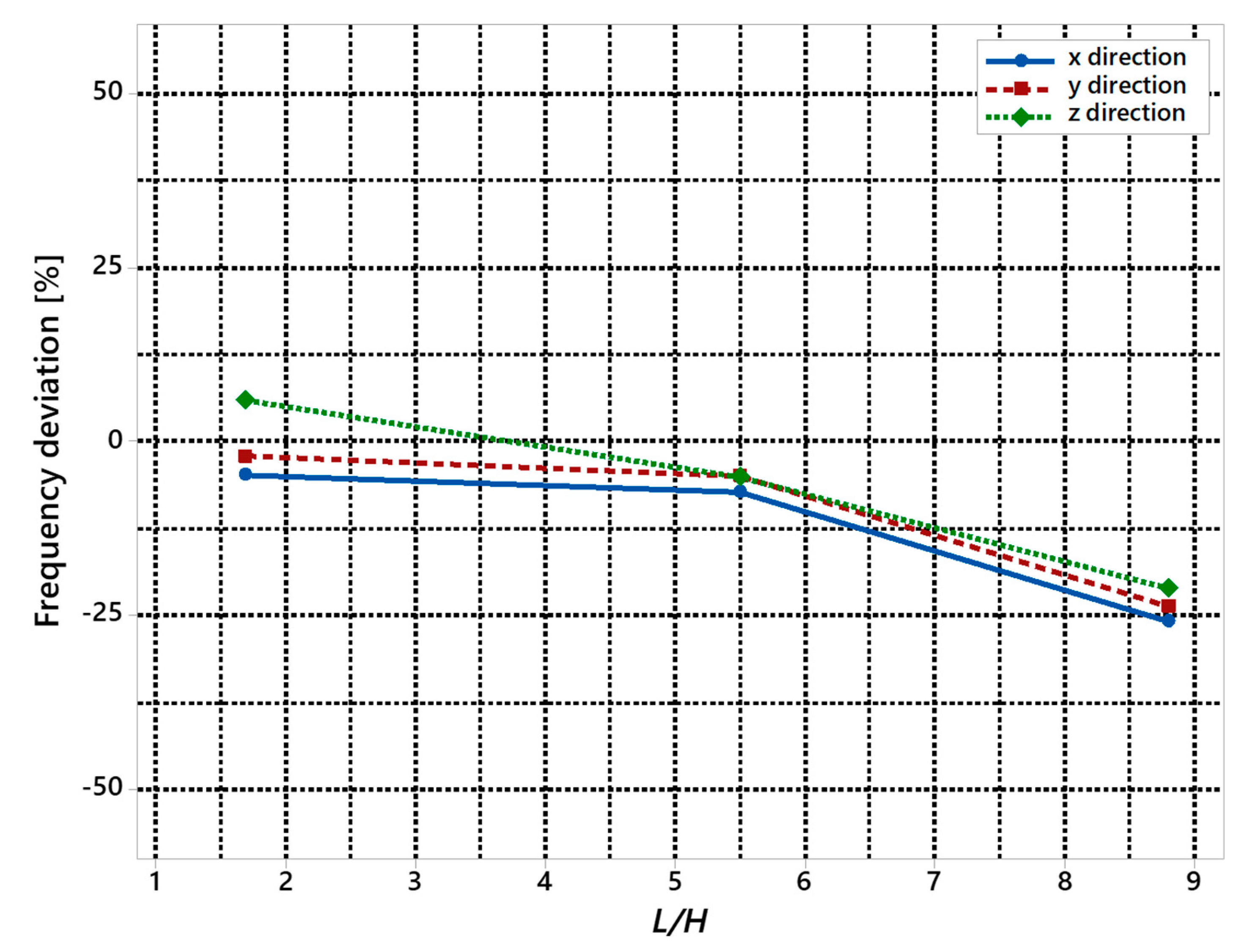
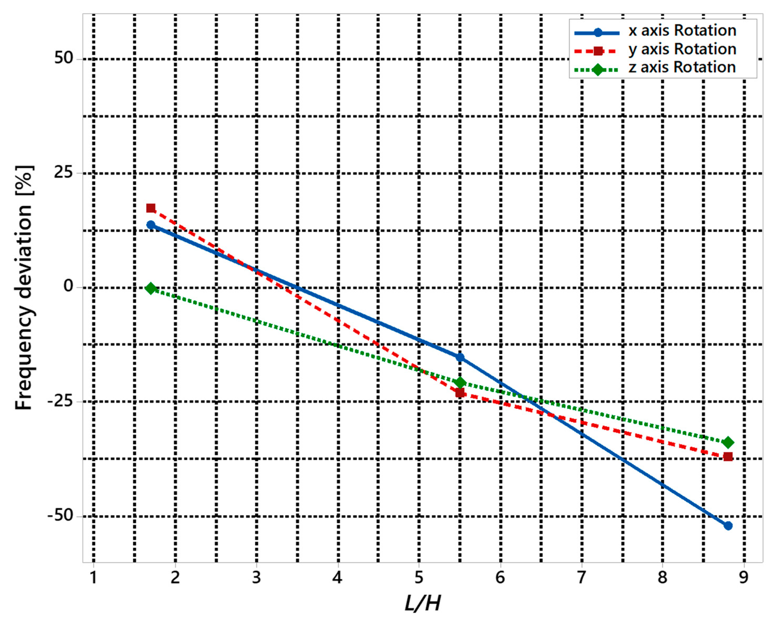
| Frequency Deviation [%] | Translation in x Direction Freq. | Translation in y Direction Freq. | Translation in z Direction Freq. | Rotation about x-Axis Freq. | Rotation about y-Axis Freq. | Rotation about z-Axis Freq. |
|---|---|---|---|---|---|---|
| Original | −4.9 | −2.2 | 5.9 | 13.7 | 17.3 | −0.3 |
| Intermediate | −7.3 | −5.0 | −5.2 | −15.3 | −23.1 | −20.8 |
| Low | −25.9 | −23.8 | −21.2 | −52.1 | −37.1 | −33.9 |
Publisher’s Note: MDPI stays neutral with regard to jurisdictional claims in published maps and institutional affiliations. |
© 2021 by the authors. Licensee MDPI, Basel, Switzerland. This article is an open access article distributed under the terms and conditions of the Creative Commons Attribution (CC BY) license (https://creativecommons.org/licenses/by/4.0/).
Share and Cite
Giorgetti, S.; Giorgetti, A.; Tavafoghi Jahromi, R.; Arcidiacono, G. Machinery Foundations Dynamical Analysis: A Case Study on Reciprocating Compressor Foundation. Machines 2021, 9, 228. https://doi.org/10.3390/machines9100228
Giorgetti S, Giorgetti A, Tavafoghi Jahromi R, Arcidiacono G. Machinery Foundations Dynamical Analysis: A Case Study on Reciprocating Compressor Foundation. Machines. 2021; 9(10):228. https://doi.org/10.3390/machines9100228
Chicago/Turabian StyleGiorgetti, Stefano, Alessandro Giorgetti, Reza Tavafoghi Jahromi, and Gabriele Arcidiacono. 2021. "Machinery Foundations Dynamical Analysis: A Case Study on Reciprocating Compressor Foundation" Machines 9, no. 10: 228. https://doi.org/10.3390/machines9100228