Unmanned Ground Vehicle Modelling in Gazebo/ROS-Based Environments

Abstract

The fusion of different technologies is the base of the fourth industrial revolution. Companies are encouraged to integrate new tools in their production processes in order to improve working conditions and increase productivity and production quality. The integration between information, communication technologies and industrial automation can create highly flexible production models for products and services that can be customized through real-time interactions between consumer, production and machinery throughout the production process. The future of production, therefore, depends on increasingly intelligent machinery through the use of digital systems. The key elements for future integrated devices are intelligent systems and machines, based on human–machine interaction and information sharing. To do so, the implementation of shared languages that allow different systems to dialogue in a simple way is necessary. In this perspective, the use of advanced prototyping tools like Open-Source programming systems, the development of more detailed multibody models through the use of CAD software and the use of self-learning techniques will allow for developing a new class of machines capable of revolutionizing our companies. The purpose of this paper is to present a waypoint navigation activity of a custom Wheeled Mobile Robot (WMR) in an available simulated 3D indoor environment by using the Gazebo simulator. Gazebo was developed in 2002 at the University of Southern California. The idea was to create a high-fidelity simulator that gave the possibility to simulate robots in outdoor environments under various conditions. In particular, we wanted to test the high-performance physics Open Dynamics Engine (ODE) and the sensors feature present in Gazebo for prototype development activities. This choice was made for the possibility of emulating not only the system under analysis, but also the world in which the robot will operate. Furthermore, the integration tools available with Solidworks and Matlab-Simulink, well known commercial platforms of modelling and robotics control respectively, are also explored.

1. Introduction

The term “Wheeled Mobile Robot” (WMR) underlines the ability of a vehicle to operate without a human presence on board or remote controlling the vehicle, in order to navigate in environments for which it is designed (ground, air, water). The form and degree of control of the vehicle provide the type and level of autonomy, ranging from the absence of automation to full automation, generally through a robotic detection system that uses model-based approaches and learning to increase their levels of driving. A definition of a mobile robot is presented by [1] that identifies their features and purpose: “A mobile intelligent robot is a machine capable of extracting information about its environment and using the knowledge of its world to move in a meaningful and safe way”. Unmanned mobile robots are being used in difficult, dangerous and/or highly unpleasant tasks to be carried out by human beings since the costs of accessibility, safety, and survival is high, or when fatigue, time, or unpleasantness are increased [2,3]. Therefore, the nowadays missions for ground, aerial and underwater-unmanned vehicles fulfil tasks like monitoring infrastructures as bridges, canals, offshore oil, and gas installation. Furthermore, mobile robotics are generally integrated into exploration, intervention, surveillance activities and, increasingly, it is taking root in new fields such as agriculture and health sector [4,5,6]. A more generic distinction allows us to understand the degrees of development reached that we will describe later, thus the “mobile robotics”, which involves all unmanned vehicles in all the environments described previously, and the “intelligent vehicles”, which deals with the mobility of people and goods on regular surfaces commonly. The basic components of mobile robots include at least one controller, a power source, a software or control algorithm, some sensors, and actuators [7,8,9,10]. The areas of knowledge usually involved in the field of mobile robotics are: mechanical engineering, responsible for the design of vehicles and, in particular, the mechanisms of locomotion; computer science, responsible for visualization, simulation, and control with algorithms for detection, planning, navigation, control, etc.; electrical engineering, capable of integrating systems, sensors, and communications; cognitive psychology, perception, and neuroscience that study biological organisms to understand how they analyse information and how they solve problems of interaction with the environment. Finally, Mechatronics, which is the combination of mechanical engineering with computing, computer engineering and/or electrical engineering [11,12,13,14,15]. Therefore, there is important “knowledge” and “know-how” from conception to experiments and implementation. The degree of development of mobile robots varies greatly according to the time and the impetus with which the research topics, technologies, and initiatives are approached. The academic community generally makes a classification as Autonomous Ground Vehicles (AGV), autonomous land vehicles (ALV) or mobile robots for vehicles travelling on land, which would be the “Intelligent vehicles”. Unmanned Aerial Vehicles (UAV) generally classified in fixed wings and rotating wings. Autonomous Submarine Vehicles (ASV) or Unmanned Surface Vehicles (USV) for those travelling below and above the surface of the water [16,17,18]. Unmanned ground vehicles (UGV) are vehicles that operate while in contact with the ground and without a human presence on board. The development of such systems began as an application domain for Artificial Intelligence research at the end of the 1960s. The initial purpose was to recognize, monitor and acquire objects in military environments. The “Elmer and Elsie” tortoises, composite acronyms for the electromechanical and photosensitive robots, respectively, were the first automatic vehicles invented by the neurophysiologist William Gray Walter at the Burden Neurological Institute in Bristol from 1947–1950, and are considered one of the first achievements of cybernetic science and as the ancestors of ground robots and “intelligent” weapons [19,20]. These turtles identified the sources of dim light and approached them, so they had locomotion, detection, and evasion of obstacles capabilities. The most notable advance of these battery turtles is their ability to make intelligent associations such as “soft light”, “intense light”, or even “light equal to a type of sound” so they were able to react to these stimuli as “conditioned reflex”, thus they are recognized as the pioneers of Artificial Intelligence (AI). Another important step in the development of mobile robots was the development of Shakey in 1966–1967, who was able to navigate from one room to another and even transport an object. Shakey, which means, “who trembles”, was capable to translate by themselves only because he can “feel” his surroundings, although to make each movement he needed a good hour of calculation. Its morphology could be described as a large camera as a head that could rotate and lean, its body was the large computer that rested on a platform with three wheels that were its means of locomotion. The robot used electrical energy, and it carried with it several sensors: a camera, a distance measuring device and tactile sensors to perceive obstacles, actuators as step by step motors. It served as a test-bed for AI’s work funded by DARPA at the Stanford Research Institute [21,22,23]. The Shakey system is the pioneer of WMRs, establishes the functional and performance baselines for mobile robots, identifies the necessary technologies and together with the Bristol turtles help define the research agenda of Artificial Intelligence (AI) in areas such as planning, vision, conditioned reflex processing and natural language [24]. The Shakey system had a new development momentum at the end of the 80s, with the implementation of an eight-wheel all-terrain vehicle with standard hydrostatic steering, able to move on roads and in rough terrain, this vehicle converted into an unmanned ground vehicle had all the electronics and software for the search of objectives and navigation [25]. The result in 1987 was a road trip guided by vision along 0.6 km at speeds of up to 3 km/h on rough terrain, avoiding ditches, rocks, trees, and other small obstacles [26,27]. Another type of WMRs called rovers serve to explore, analyse and photograph the surface of the planet Mars, the first was named Sojourner, meaning “hero” or “traveller”, launched in 1997. It was active from 6 July to 27 September. Its mission was to explore Mars in a radius of action of 20 m around the landing platform called PathFinder. This platform served as communication with the land. Later, Spirit and Opportunity, two twin rovers were launched in January 2004, again to explore Mars in a wider area. Then, Curiosity, sent in August 2012 in the mission Scientific Laboratory on Mars and it is expected that in 2021 the rover call Mars2020 will be sent in mission. The development of increasingly performing robots, capable of performing missions effectively, goes hand in hand with the development of robust computational platform and tools to be used for rapid prototyping, evaluate robots design, simulate virtual models and sensors, provide and evaluate models and controllers, capable of satisfying the expanding demand and the renewed interest in robotics [28,29,30]. It is also important for developers and implementers to be aware of the available platforms, methods, algorithms, hardware components that are most used, as well as their underlying physical and numerical paradigms, advantages, and disadvantages [31,32]. Those are the reasons why in this paper we present a robotics framework from a broader perspective, with an emphasis on open-source ones. The main characteristics and components are discussed and compared. In 2012, a paper presenting MIRA middleware did a comparative benchmarking of the robotics platforms available at this moment. Updated general information of these platforms and their basic characteristics are summarized in

Table 1. Middleware platforms summary.

ROS	Robot Operating System	http://www.ros.org/	For complex mobile and manipulator robots, based on algorithms and actuated sensing. Distributed.
MIRA	Middleware for Robotic Application	http://www.mira-project.org/joomla-mira/	Distributed applications of several different processes (algorithms for certain task) on different machines (either in real time).
YARP	Yet Another Robot Platform	http://www.yarp.it/	Modular, code reuse, transport-neutral interprocess communication based on Ports with different protocols.
Urbi	Universal Robotic	https://github.com/urbiforge/urbi	UObject (C++ API) for drivers and algorithms designed and exposed to urbiscript (event-based) used to connect components in an application. Distributed at runtime.
LCM	Lightweight communications and marshalling	https://lcm-proj.github.io/index.html	platform- language independent, publisher/subscriber, low-latency message passing systems for real-time robotics research applications
Player	Player/Stage Project	http://playerstage.sourceforge.net/index.php?src=index	Fits well for simple, non-articulated mobile platforms. Offers more hardware drivers, provide easy access to sensors and motors on laser-equipped.
MOOS	Mission Oriented Operating Suite	http://www.robots.ox.ac.uk/~mobile/MOOS/wiki/pmwiki.php/M	star-shaped topology network. Data as named messages stored in MOOSDB. Other clients can fetch also the history of changes.

.

The benchmarking could help to realize which platform will fit better to specific robotics’ needs and purposes. It is even possible to combine them for large robotics environments or projects. Robotic software must cover a broad range of topics and expertise from low-level embedded systems, for controlling the physical robot actuators, all the way up to high-level tasks such as collaboration and reasoning [33,34,35]. The many layers of computation must seamlessly be able to communicate and integrate with each other for a robotic system to function successfully. Additionally, several tasks, such as mapping and navigation, are common to many robotic applications. Then, a layer of software above the operating system but below the application program appears in the market to wrap this complexity and to provide a common programming abstraction across a distributed system [36].

Table 2. Middleware advantage summary.

Portability	Common programming model across language and/or platform boundaries, as well as across distributed end systems
Reliability	Can be reused and optimized with confidence over many applications
Managing complexity	Low-level programming abstractions can be made more accessible through suitable (possibly object-oriented) libraries. However, programming combinations of these abstractions can be excessively tedious and error-prone. Programming within the context of pattern aware middleware can drastically reduce both chances of introducing errors into the code, and the amount of pain that the programmer must endure when implementing the system (Schmidt et al., 2000).

summarizes the advantages of these platforms. The primary research areas are Control, Locomotion, Machine learning, Human-Robot Interaction (HRI), Planning, Mechanical design, Cognitive robotics and Mathematical modeling. The primary application fields instead are Humanoid robotics, Mobile robotics, Multi-legged robotics, Service robotics, Industrial robotics and Numerical simulation of physical systems [37,38]. Gazebo-ROS is a powerful combination used by the robotics community in general for its ability to simulate with credibility their environments and the flexibility, robustness, and availability of common features for thefts, capable of supporting complex distributed environments with multiple robots performing tasks in a coordinated manner [39]. That being said, it is easy to understand that this management of complexity that allows both flexibility and integration with other robotic environments requires some solid knowledge to exploit the full potential of this Gazebo-ROS platform [40,41]. The authors for some time have been using 3D design software to develop detailed models for dynamic simulations. In particular, the use of the SimMechanics link tool allows the creation of rigid multibody models in the multi-domain simulation environment. In this environment, it is possible to build multi-domain models as in the case of mechanical parts driven by electric actuators. These tools therefore make it possible to obtain a good model with regard to geometry and mass distribution. However, the force fields that surround the system we want to analyse are left to the designer who has the task of modelling the forces present at the interface between the system and the environment. The Gazebo simulation environment instead takes into account system-environment interactions allowing a more truthful study on the dynamic behaviour of the system under analysis. In literature, it is easy to find examples of robotic simulations in Gazebo through the use of multibody models supplied directly by the manufacturers. Instead, it is more difficult to find applications with custom robots. For this reason, we decided to test this platform by recreating a mobile robot that we have in our laboratory, in order to test the strengths and weaknesses of this prototyping environment. The paper is organised as follows. In Section 2, we describe the Gazebo robot simulator and its potential. Moreover, the design process for creating the multibody model is shown together with the modeling of the contact forces between wheels and floor. Section 3 describes the co-simulation activity conducted by using Gazebo 10.0 and Matlab 2018b softwares. Finally, in the last sections, we present our considerations.

2. Materials and Methods

Gazebo development starts as part of a Ph.D. research project. After 2009, it had been integrated with ROS in a PR2 robot at Willow Garage Company (Menlo Park, CA, USA), which becomes the most important financial support since 2011. Now, the version 10 is on development, and it is expected to be launched by January 2019. V.11 is already describing new functionalities and is expected to be released by January 2020. Therefore, respecting the promise, Gazebo launches a new major version once a year, with a useful life of two and five years for even and odd versions, respectively [42]. Gazebo is a powerful 3D simulator, capable of being integrated into various robotic platforms; however, it is the natural complement of ROS. One of the recognized strengths is the ability to incorporate different physical engines, each of which has their own level of development and some has a marked orientation to the simulation of certain types of robots, as in the case of Simbody for humanoids [43]. For the selection of the various engines, it will be enough to invoke them during the launch in the scripts that invoke the packages to be executed with their respective parameters. Another important component during robotics simulation is rendering this management of the appearance of the moving image. Both the rendering and the physical engine will make the simulation plausible; even so, there is a compromise to achieve between accuracy of response to the physical phenomenon of the modeled environment and the capacity to respond in computational terms [44]. A simulator must synthetically simulate the environment from a visual perspective as physical (laws of physics) of the environment they represent. To this graphical environment, Gazebo calls it “world” where the various static and/or dynamic objects must be represented; it identifies them as “model” that, according to the mission to be developed, will be rich in terms of set design and/or dynamism. Both the “world” and the “model” have a series of configuration parameters to which it is possible to access from the graphic Gazebo environment, through plugins (executable with specific functionalities) or through control platforms such as ROS or others [45,46]. Described in this way, everything seems very simple, but working in a virtual environment simulating the basic capabilities of a mobile robot is not as simple as it seems. These tools are powerful because they just hide all this complexity in the functionalities they offer and allow us to interact with them through configurable parameters, which in the case of the physical environment are interrelated, and, in many cases, have immediate implications on each other. It is therefore important to have knowledge of the basic concepts and laws that govern them, to understand how they have been incorporated into these tools and what they really mean in each environment [47]. Thus, Gazebo is a three-dimensional open-source dynamics simulator for single and multi-robots’ mechanisms, for inside and outside environments. Despite the fact that it was created to close the gap of realistic robot simulation in outdoor environments, the users mostly use it for indoor simulations. Gazebo attempts to create realistic worlds for the robots, relying heavily on physics-based characteristics; what it means is that, when the model is pushed, pulled, knocked over, or carried “reflecting the physics” [48].

The general structure (see Figure 1) remains simple and almost unchanged since it was presented in 2004 because it relies on third-party software packages as ODE for articulated rigid bodies dynamics and kinematics; and system independent visualization toolkit, called GLUT, for the creation of 2D and 3D interactive applications (over a standard library OpenGL). This characteristic makes Gazebo an independent platform, which permits, for example, to add Dynamics Engines as Bullet, Simbody, and DART for different versions and platforms; however, the original ODE remains the default engine [49]. By doing so, Gazebo’s major feature is the creation and addition of models, which are virtual dynamic objects such as robots, actuators, sensors, ground surfaces, buildings or other stationary objects, relying on ODE Dynamics by means of Newton–Euler equations and First-order time integrator for Motion; Frictionless joints for Constraints; Perfectly inelastic collision for Collisions and Friction pyramid for Contacts. The World represents these models and environmental factors as gravity, lighting, and so on. Finally, user Interfaces are used by client programs to communicate and control models [50]. As reported in the Gazebo aArchitecture scheme, there is a division between server and client, which are provided by two executable programs “gzserver” for simulating the physics, rendering, and sensors; and “gzclient” for a graphical interface to visualize and interact with the simulation. The client and server communicate using the Gazebo communication library Google Protobuf and boost::ASIO, for message serialization and transport mechanism, respectively [51]. The Gazebo features are described on their official website and there are also tutorials and models to use in order to understand such powerful environments. For modelling, Gazebo uses SDF (Simulation Description Format), which is an XML format to describe objects and environments, capable of describing all properties of robot model (links, joints, sensors, plugins), static and dynamic objects, lighting, terrain, and even physics. Links are described by Inertial (mass, a moment of inertia), Collision and Visual (geometry) which are used by physics, collision and render engines, respectively. Joints connect two links and are used to constrain their movement, limiting the DOF (degrees of freedom) by the type (revolute, prismatic, revolute2, universal, ball, screw) of their configuration [52]. Because of the above, the framework, conceived as a robotic platform and a work environment, has been developed under the guidelines and scope of the chosen base robotic middleware call GAZEBO-ROS and the integration capabilities that expand its usage possibilities [53]. It is also known in the robotics community how several difficulties are faced while developing robotics applications due to the heterogeneity of the concepts in the field. In fact, in the case of mobile robotics, they must master the details related to the locomotion medium of robots, its morphology, and its sensors. In addition, the variability of the hardware makes the robotic applications fragile, which means that a hardware change in an already developed application would imply the rewriting of the code [54]. To respond to the observation of hardware variability, some robotic middleware such as ROS, MIRO, and PyRO, proposed abstractions of the hardware components in relation to the technical details of these; it is thus possible to encapsulate specific data and instead provide higher level data. However, these abstractions are still at a low level and do not allow the isolation of some hardware components’ changes [55]. After evaluating the different alternatives reported in Table 1, we choose Gazebo-ROS as the base middleware environment because it supports the simulation and control of complex robotic missions, thanks to its easy integration with tools such as Simulink, MATLAB, and Solidworks.

Wheeled Robot Modelling in a Gazebo-Based Environment

The mathematical modelling of mobile robots, in general, is carried out in order to understand their behaviour in an established acting environment. This mathematical formulation describes the kinematic and dynamic models that will serve as the basis for the design and control of robots in general [48,56]. When designing mobile robots, the aim is to achieve models with levels of reliability and manoeuvrability necessary to fulfil the desired functionalities, such as precision and speed, while having stable mechanical structures [57]. Furthermore, such analysis, depending on the morphology, allows to study the best arrangement of the components like sensors and actuators, in order to fulfil the purpose of the robot. Kinematic and dynamic characteristics are expressed in mathematical formulations that may or may not consider the geometry of the robot [58,59]. It is also possible to develop several mathematical models to represent the same mobile robot, each of them having different utility depending on the functionality that we want to achieve, observe or analyse. The WRM, reported in Figure 2, is the prototype of wheeled mobile robot, designed and assembled in the laboratory of Applied Mechanics of the Department of Industrial Engineering of the University of Salerno. It has a conventional geometry that facilitates the study of control design application, identification techniques and autonomous navigation algorithms. Furthermore, it is normally used for educational activities in order to provide a first approach to robotics for our students [60,61]. The chassis of the three-wheeled mobile robot is made of metal-acrylic and has a combination several sensors for performing different tasks. For obstacle avoidance, SRF05 and SRF06 ultrasonic sensors are installed on the vehicle together with three other sensors on the front dedicated to object recognition activities. Such ultrasonic sensors have a range of claimed detection distance ranging from 2 cm to 450 cm and from 2 cm to 510 cm, respectively, with an accuracy of 2 mm. The two fixed-axle wheels are driven by electric DC motor-reducers with digital incremental encoders. The system is controlled, depending on the experimental activities, by an Arduino-Galileo, a board based on the Intel Quark SoC X1000 application processor or an Arduino Mega2560. The sensors, actuators, and microcontrollers work with a 12-volt battery (see Figure 2).

On the rear, a castor wheel gives stability to the rover and allows the chassis to remain horizontal. The traction-steering system associated with our robot allows for independently managing the linear and angular speed, with the advantages derived from the mechanical structure and the control electronics, make this configuration a simple solution that can be subjected to various laboratory tests [62,63]. These advantages could be summarized as follows:

• simple mechanical structure that facilitates kinematic modelling;
• low manufacturing costs;
• facilitates calculations of safe space (free of obstacles) by using the biggest dimension of the rigid platform as “robot radio”.

It facilitates the calibration of various components that tend to present systematic errors such as unequal wheel diameters, wheel misalignment, effective contact points of the wheel with the floor, and loss of efficiency of encoders [64]. However, the disadvantages are:

• difficulty moving on uneven surfaces;
• the loss of contact of one of the active wheels with the ground can change the orientation sharply;
• sensitivity to the sliding of the wheels, due to slippery floors, external or internal forces.

In order to create a good model capable of reproducing the dynamic behaviour of the WMR, we decided to build a multi body model of the rover by using a CAD assembly file from Solidworks software [65].

Such Cad files, through the use of Blender software, allowed us to obtain a multi body model of the rover for the Gazebo environment (see Figure 3). Instead, in the Gazebo-ROS platform, it is common to have a model in a “.urdf” or “.urdf.xacro” file types are used in “RVIZ”, a visualization tool heavily used for testing and debugging as reported in Figure 4. Once the system has been modelled, we concentrated on the force fields that surround the robot in the environment in which it is located. In general, the kinematic modelling of a rover depends on the physical characteristics of the robot and its components [13,14,15]. Their characteristics will make them suitable for a certain task, and vice versa, the task itself will be the one that will determine in a first stage the structural particularities of the vehicle. The design must consider the mobility required to carry out the assigned task, energy efficiency, weight/load ratio, dimensions, and manoeuvrability; in the same way the environment of ground operation [66,67]. The ground mobile robots distribute their traction and steering systems on the axes of their wheels according to the demands of speed, manoeuvrability, and characteristics of the terrain in which they must perform. The capacities required according to the missions will determine the type of more convenient wheels, the number and the arrangement; as well as the traction and direction system, and finally the physical form of the robot. Therefore, several mathematical models can be used to represent the kinematic characteristics of the robot, by incorporating various properties that will be of interest to achieve or observe the particular behaviour.

Based on these models, it determines the different positions in which it is located and the speeds at which it moves. For our rover, we have chosen standard wheels that meet the three conditions defined for this design:

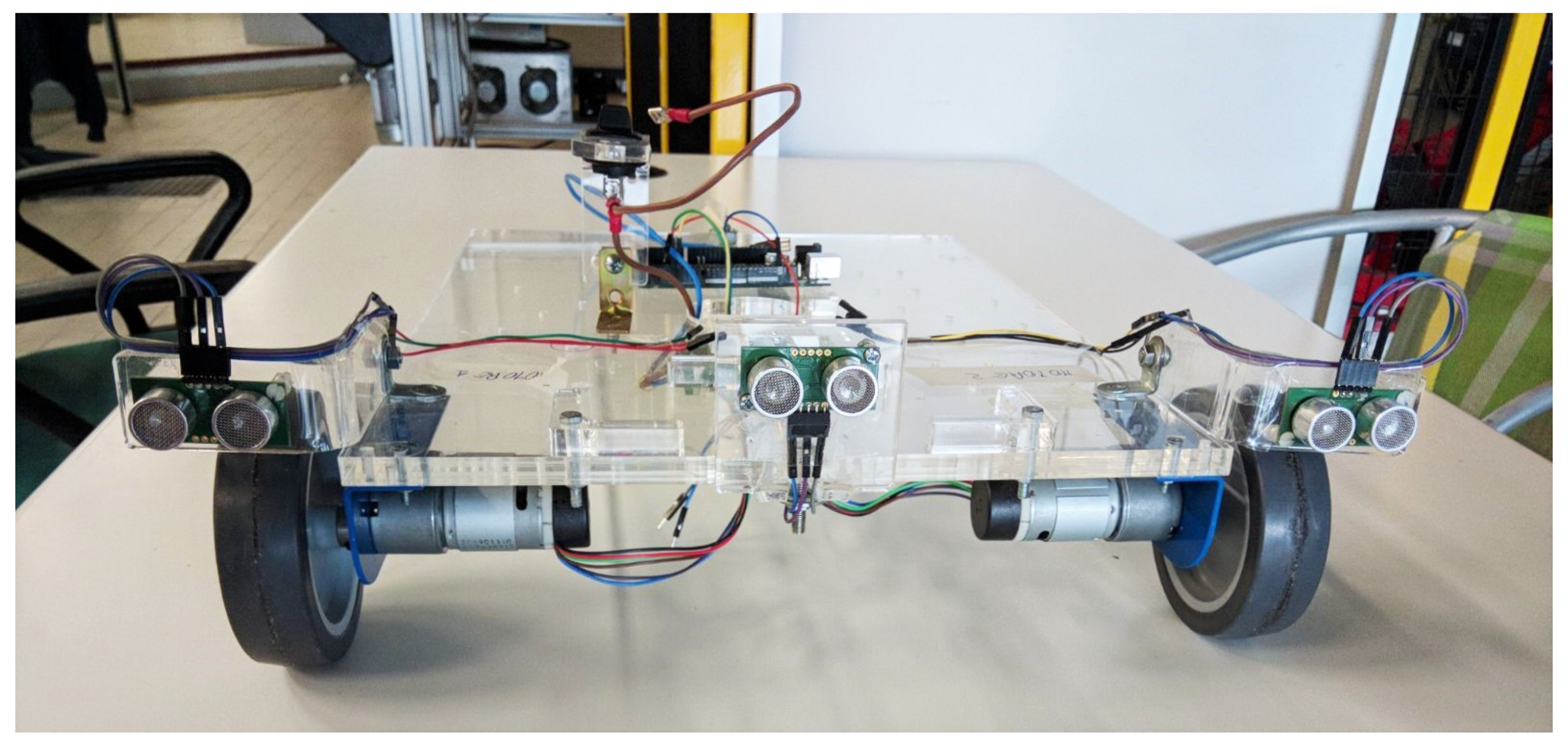
• The front wheels are equidistant in the common axis of rotation, without lateral variations, while the castor, located in the rear, provides a pure rotation contact between it and the ground without causing slips in the vehicle when moving.
• The mechanical design of the two front wheels as “fixed” confers a speed restriction in the driving direction (only forward and backward), while the castor wheel has free movement.

The two front wheels are controlled by the two actuators, while the idler wheel is passively controlled, meaning that it is influenced by the general movement of the chassis and does not provide an additional speed restriction in the movement of our robot [68]. For our vehicle, the origin of its frame on the coordinate system of reference has been located at the midpoint of the line that joins the two fixed wheels and an axis coinciding with this line forming the orthogonal [69]. Three possible movements for vehicles that use this technique are revealed in literature—the first straightforward movement when the speeds of both front wheels are equal, the second a rotation in its central axis (the midpoint of the common axis) when the wheel speeds are equal but in opposite directions and third a rotation around one of the wheels, when one of them has zero speed. There is no possibility for lateral movement; this restriction is called singularity. The other singularities related to the errors in the relative speeds of the wheels, or the small variations in the level of the ground are mitigated by the castor wheel [70]. When the front wheels act independently, i.e., by varying their speeds, we will make the mobile robot move with linear trajectories or with turns, to the right or to the left depending on the lower speed value of one of the wheels. All movements are appreciated with respect to the frame of the vehicle. If we want the vehicle to move in a circle, the robot must turn around a point that is along the common axis of the right and left wheels. The point on which the robot rotates is known as instantaneous curve center [71]. The mobile robots need mechanisms of locomotion that allow them to move through the environment to carry out the assigned mission; these mechanisms of locomotion on land can be different and, depending on the choice made and implemented, the robots can walk, jump, run, slide, crawl and roll. The mechanism of locomotion on the ground preferred and chosen by researchers and the robotics industry has been by far the wheel, being mechanically simpler and more efficient, especially on flat surfaces [72]. The key components that influence the total kinematics of the WMR are undoubtedly the wheels, so the selection and the arrangement of these in the vehicle are important. There are four types of wheels commonly used, with advantages and disadvantages, and have very diverse kinematics, these are:

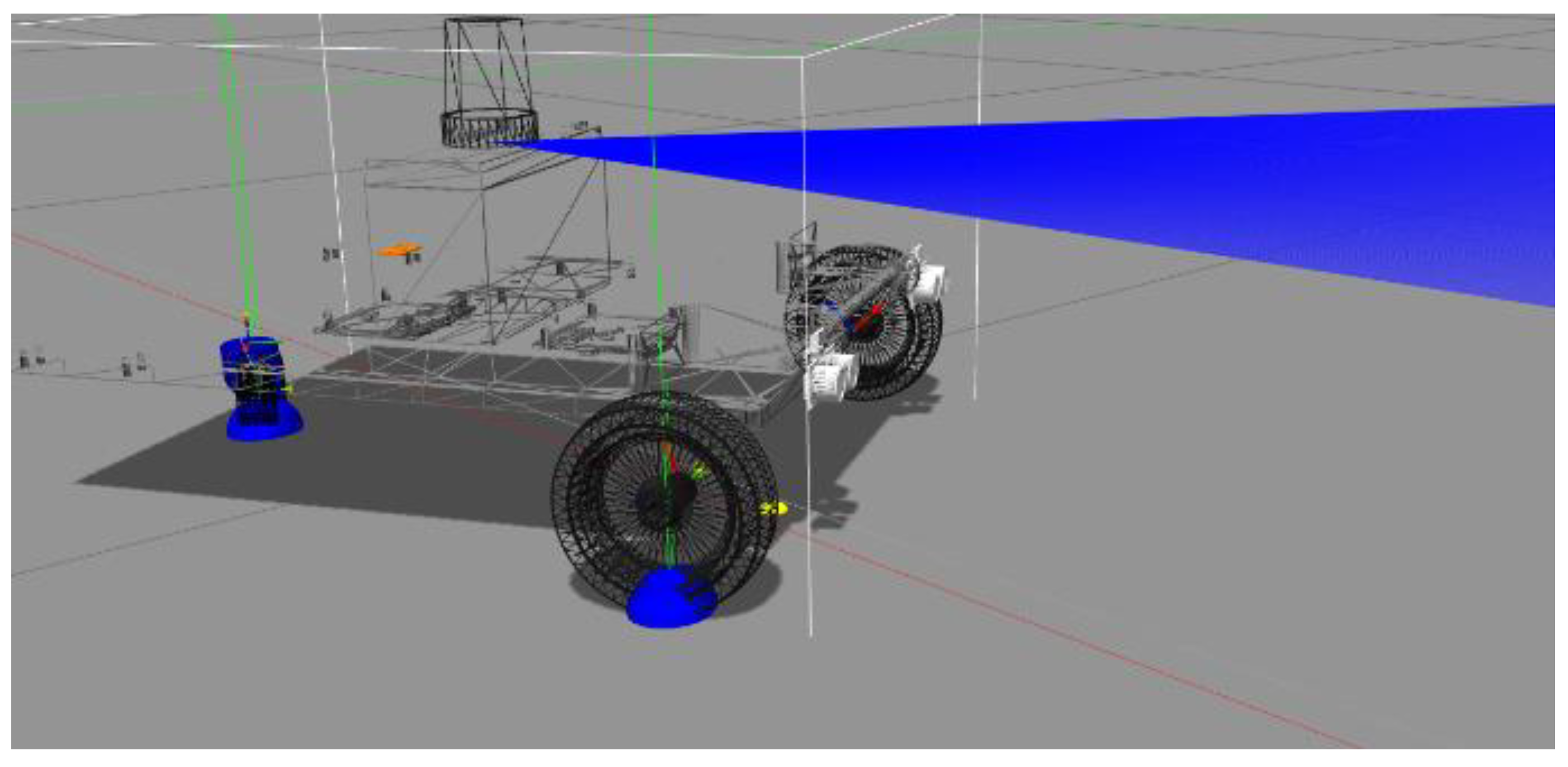
• Standard wheel: two degrees of freedom, rotation around the wheel axle (usually motorized) and the point of contact;
• Rotating wheel: two degrees of freedom, rotation around a controllable displaced joint;
• Swedish wheel (Swedish): three degrees of freedom, rotation around the wheel axis (usually monitored), around the rollers or bearings, and around the point of contact;
• Ball or spherical wheel: technically difficult realization.

According to the selection and disposition of this type of wheels, the WMR will have different degrees of freedom, which will characterize its manoeuvrability, how easily it rolls in a straight line, or makes turning motions. Omnidirectional robots have the maximum manoeuvrability in the plane. Such behaviour is granted by the Swedish wheels; this freedom of movement can also be achieved in the plane with steerable wheels centered with traction and steering motors that control each of the wheels in an independent and synchronized way through mechanical systems of belts or electronic means. The last option has a degree of mechanical and electronic complexity to achieve good coordination between the wheels—requiring also having a complex control algorithm, so its use is very limited [73]. The efficiency of wheeled robots depends to a large extent on the quality of the terrain, particularly the smoothness or hardness of the terrain, the type of surface (flat or non-flat), and the number of obstacles (free or dense). Thus, conventional vehicles on wheels usually move on regular and hard enough terrain, while, for irregular terrains, track wheels with gears and adapted diameters are required. For example, a robotic vehicle for floor cleaning missions will have an appropriate configuration to the displacement on polished and/or carpeted floors in general, while the ground mobile robots that will have to attend to monitoring requests in devastated places will have a diverse configuration that can adapt to irregular terrain, with debris and other conditions that will limit its displacement. In Gazebo, when two objects collide, like wheels rolling on a surface, a friction force is generated; to manage those forces, there are physical engine systems defined in simulator software. Gazebo has different physics engines including ODE, Bullet, Simbody, and DART, and it is possible to choose one through the <physics> element in a .world file. These physics parameters’ configurations permit to personalize the characteristics and values needed in the simulation environment through profiles, available via the C++ API or gz command line tool [74]. The performance, accuracy, and general behaviour of physics simulation depend to a great degree on the physics engine and how the main parameters of them are defined. Some of these parameters are shared between the different physics engines supported by Gazebo, like maximum step size and target real-time factor. To manage them, Gazebo has a physics preset manager interface that offers a way to easily switch between a set of physics parameters and save them into Gazebo’s .sdf robot configuration. This physics configuration could be called and redefined at any plugin creation by calling $world\to GetPresetManager\left(\right)$ in C++ programs. The default physical engine in Gazebo is ODE. In such engine, the main friction elements are composed of two parameters, “mu” and “mu2”, friction coefficients along the contact surface, which stands for:

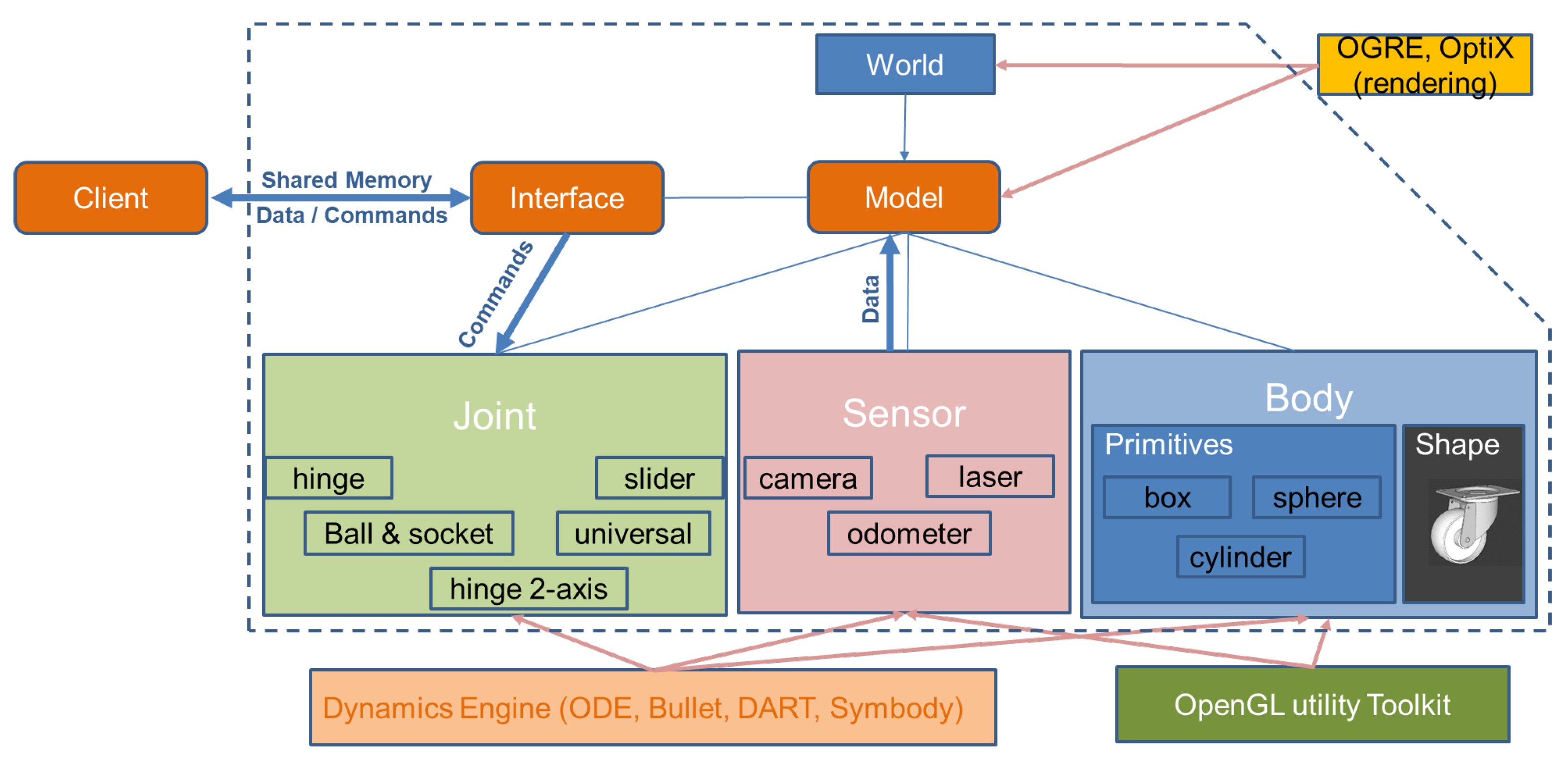
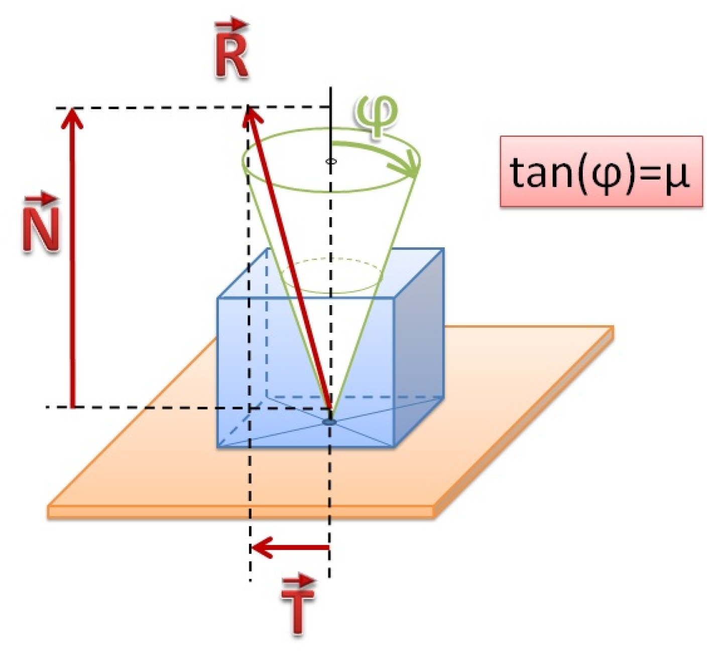
• “mu” is the Coulomb friction coefficient $\mu$ for the principal contact directions or the first friction direction;
• “mu2” is the friction coefficient for the second friction direction (perpendicular to the first friction direction).

Another important element that works closely related to each other is:

• the two contact stiffness $k_p$ and damping $k_d$ for rigid body contacts; those are defined as Gazebo’s links parameters, “kp” and “kd”;
• the joint stop constraint force mixing (cfm) and error reduction parameter (erp) used to simulate damping.

In simulation, the dynamics world (dWorld) stores bodies (dBody) and is responsible for computing where they are at any given time. Thus, the “state” of all the rigid bodies are recalculated at every “step time”, meaning that, at a selected period of time, a new position vector (x,y,z) and linear velocity (vx,vy,vz) of the body point of reference that usually correspond to the body’s center of mass, are calculated, in addition to their orientation, represented by a quaternion (qs,qx,qy,qz) or a 3 × 3 rotation matrix; and their angular velocity vector (wx,wy,wz) [75]. When two bodies are close enough, the simulator will call a function to determine which bodies or “geometries” are potentially intersecting/colliding. It creates a collision space (dSpace) to store geometries corresponding to bodies (dGeom), flags those bodies, and actually specifies the maximum of contact joints to create, so that the dynamics world can adjust its velocity accordingly. Each body has its collision space, which is tested for collisions against each other before and then dGeoms inside them are tested in case these are nested. ODE has its own built-in collision detection with collision spaces and dGeoms that will return a number of “Contact Joints” that define where the bodies are in contact. All contact joints that ODE finds are placed in the “contact” array. The functions that are called for space creation and flags control look like:

• void dSpaceCollide (dSpaceID space, void ∗data, dNearCallback ∗callback);
• int dCollide (dGeomID o1, dGeomID o2, int flags, dContactGeom ∗contact, int skip).

The CFM (Constraint Force Mixing) and ERP (Error Reduction Parameter) can be independently set in many joints; both are floating point values between 0.0 and 1.0. The first one will permit a degree of joint constraint violation, and collisions will have a “spongy” look; the second one refers to how much “joint error” is fixed in each time step. Gazebo tutorials suggest default values as 0.2 and 0.8 for both of them, respectively [76]. ERP and CFM can be selected to have the same effect as any desired spring and damper constants. If you have a spring constant $k_p$ and damping constant $k_d$, then the corresponding ODE constants are:

$$ERP=\frac{h{k}_p}{h{k}_p+k_d},$$

$$CFM=\frac{1}{h{k}_p+k_d},$$

where “h” is the step size.

Between each step time, the user can call functions to apply forces to the rigid body. These forces are added to “force accumulators” in the rigid body object. It means that dynamic steps when the next step time happens start with the sum of all the applied forces to be used to push the body around; then, a collision detection is called, if ODE finds a possible collision, it creates a “Contact Joint”. Gazebo’s friction has models: cone friction, pyramid friction, and box friction. Thus, depending on “$friction\_model$” variable setting, the specific pieces of code will set the parameters and call the functions named needed to tread the collisions. If it is not specified, the $dxConeFrictionModel$ will be used. The Coulomb friction model has a simple relationship between the normal and tangential forces present at a contact point [77]. The rule is:

$$|F_T|\le \mu |F_N|,$$

where $F_T$ is the Tangential force vector, $F_N$ is the Normal force vector and $\mu$ is the friction coefficient.

In ODE’s friction cone model (see Figure 5), to achieve the “adhesion mode”, the vector of the total friction force must be inside the cone, and the friction force must be enough to prevent the contact surfaces from moving with respect to each other. If this vector is on the surface of the cone, then the contact is in “sliding mode” and the friction force is usually not large enough to prevent the surfaces in contact from sliding. The parameter “mu” represents the maximum ratio of tangential force to normal force.

In this model, there are currently two approximations to choose from:

• “mu” is the force limit to be chosen appropriately for the simulation, which means that the maximum friction (tangential) force that can be present at a contact, in either of the tangential friction directions. This is rather non-physical because it is independent from the normal force, but it is the computationally cheapest option.
• The friction cone is approximated by a friction pyramid aligned with the first and second friction directions. First, ODE computes the normal forces assuming that all the contacts are frictionless; then, it computes the maximum limits $F_m$ for the friction (tangential) forces from $|F_m|\le \mu |F_N|$ and then proceeds to solve for the entire system with these fixed limits.

This differs from a true friction pyramid in that the “effective” mu is not quite fixed and can be set to a constant value around 1.0 without regard for the specific simulation.

ODE will automatically compute the first and second friction directions; however, it is possible to manually specify the first friction direction in the model description file “.sdf” or in “.urdf” if it is used in a Gazebo-ROS environment. The two objects in collision specify their own “mu” and “mu2”. Gazebo will choose the smallest “mu” and “mu2” from the two colliding objects. The valid range of values for “mu” and “mu2” is any non-negative number, where 0 equates to a friction-less contact and a large value approximates a surface with infinite friction. Tables of friction coefficient values for a variety of materials can be found in engineering handbooks or through an online toolbox.

The cone friction model algorithm computes the corresponding $h{i}_{act}$ and $l{o}_{act}$ for friction constraints. For each contact, we have $lambd{a}_n$, $lambd{a}_{f1}$, and $lambd{a}_{f2}$. Now, couple the two frictions and, to satisfy the cone Coulomb friction model tangential velocity at the contact frame:

• v_f1 = J_f1 ∗ v
• v_f2 = J_f2 ∗ v
• v = sqrt(v_f1^2 + v_f2^2);
•  
• if (v < eps)
•  
•    lo_act_f1  = 0;
•    hi_act_f1  = 0;
•    lo_act_f2  = 0;
•    hi_act_f2  = 0;
•  else
•    hi_act_f1 =  abs(v_f1) / v  ∗  (mu ∗ lambda_n);
•    lo_act_f1 = − lo_act_f1;
•    hi_act_f2 =  abs(v_f2) / v  ∗  (mu ∗ lambda_n);
•    lo_act_f2 = − lo_act_f2.
•  end

For our wheel–terrain interaction model, we consider nondeformable wheels because our real WRV has solid plastic materials and the weight load charge during operation in simulation and real experiments would not be that important that it would change the rigidity. The indoor environments selected were on solid pavement; therefore, the wheel–terrain interaction can be reasonably approximated as a point contact, which permits the use of a classical Coulomb friction to describe bounds on available tractive and lateral forces as a function of the load (basically power, motors, sensors, actuators, and other components carried on) with a coefficient of friction in Gazebo-ROS.

In our case, based on our 3D model characteristics, the charge of the load carried on, and the wheel–terrain interaction hypothesized, we configure the values of mu and mu2 with the same value of 0.8 for either two frontal wheels and for the back caster one in the WMR .urdf configuration file. We configure <kp>100000000.0</kp> and <kd>10.0</kd> for all three wheels. In addition, in the .world file, the element <constraints> for our simulated environment with the values of <cfm>0.00001</cfm> and <erp>0.2</erp>.

3. Results

The described capabilities required by autonomous vehicles, such as mobile robots, can incorporate techniques that allow them to estimate their position and location build or use a map, navigate in them or without any knowledge of the environment, identifying brands, planning routes and following them [78]. To do so, it is necessary to identify the mobile robot in an abstract way, as a point (x, y) in a continuous or delimited space of two or three dimensions, generally, a Cartesian plane, to describe its state also called pose (position and orientation). When the mobile robot moves, it changes its position and orientation, but it must do so through free spaces; each free space is called Cfree and could house the robot in its path.

It is also possible to represent the mobile robot as a set of rigid bodies, for example, the WMR have the chassis, the wheels, the actuators and sensors on board and communication equipment. With these three fundamental abstractions “space”, “pose” and “free space”, we can create techniques for path planning, location, perception or sensing, mapping and SLAM (simultaneous localization and mapping) to give the mobile robot a safe journey. An example of such tecniques has been reported in Figure 6. It is possible to observe the rover in the Gazebo environment called “empty world” on the left side of the screenshot, in the middle the plot of the executions aligned with the first three points tours with precision by our WMR. The first three points correspond to a simple square that we prepare as a mission to fulfil during WMR navigation; finally, on the right side of the screen capture, it is possible to see the main components of the Matlab–Simulink control program for this way-points navigation activity in Gazebo. The virtual model of our unmanned vehicles was made using an XML-like language (Xacro, URDF, and SDF), compatible with the Gazebo simulator environment. Despite the primitives shapes of our rover, it was not easy to construct the model directly on Gazebo’s building editor, due to the limited building tools. Thus, we use two strategies for modelling; in both, it was necessary to pay special attention to geometry and relationship of all the components. In addition, we must adhere apply, as much as possible, to the three most important ROS standards—one related to Standard Units of Measure (REP-103), another to Coordinate Conventions (REP-105, in robotics, the orthogonal coordinate systems are commonly called frames) and finally ROS Package Naming (REP-144) [79]. The first strategy was to download and modify a xacro file from another simple wheeled mobile robot provided by the ROS community on the GitHub platform. In our case, it was a four-wheeled vehicle. The second strategy was to design our WMR model in SolidWorks and import it as a .dae file through a plugging that converts a 3D model into URDF. Comparatively, both roads give as a virtual 3D model, but the time expended to create a model from scratch and to export an adequate model from a CAD tool is both comparable time-consuming. Both strategies give us a virtual 3D model; the second one generated in Solidworks could be exported with the links’ inertial information calculated directly from the model, as well as with the sensors and their characteristics. In this way, the model is completely ready to use; however, the plugin used to convert to an urdf or sdf file was not a straightforward endeavour; there had been a lot of workarounds to do in order to align the reference frames and the poses. The key process in taking a CAD model in SolidWorks and bringing it through the exportation process into Gazebo for simulating requires to have a complete description of the robot and its components. In a Gazebo-ROS platform, there are two kinds of files, Universal Robot Description Format (URDF) and Simulation Description Format (SDF). The URDF file type is used heavily in ROS for visualizing and controlling and SDF files are what Gazebo uses when performing the simulation. Before importing the model CAD into Gazebo, it is advisable to simplify the assembly as much as possible so that there are no errors during the export process. Thus, the bodies are assembled together if those will not act independently in any way; the parts of the body that will participate to the motion are considered as a rigid body and must be identified correctly. To export from SolidWorks to Gazebo, it is necessary to generate the meshes for the main body and all the components. Then, it will be necessary to check that the various parts are positioned in the right way by opening the robot in Gazebo. If the collision models are not in the same place as the visual model, there may be an error with the origins in the SolidWorks model. To make it easier, it is necessary to place the origins of the visual and collision model in the same place. It is also preferable to check the meshes in software as a Blender and move the part origin to the exact position if necessary.

The flowchart, reported in Figure 7, shows the procedures to follow in order to achieve a multibody model for the Gazebo environment. The first process uses a plugin in Solidworks, called SW2URDF, to get a kind of ROS package to be used with Gazebo-ROS; once compiled (catkin process), the .urdf file is available to be used in any ROS application. The second process is a procedure to follow called Gazebo Exporter that give .sdf files with the robot description all the files needed to be launch in Gazebo simulator. There is a small application, a plugin in Solidworks, which helps with the task of getting the files needed for Gazebo-ROS. To work with, the plugin sw2urdf must be installed and configured. Immediately after the button exporter is activated, “Export to URDF” is available from the file menu. Gazebo Export generates an SDF file, a graphical scheme helps to choose the components of the main body. The first step is to choose the model name (without spaces), select the base plane and the axis direction. Another important thing to do, on the first screen, is to insert the various links to the base they are attached to. For each link, it is necessary to specify the name, collision and visual component (selecting the component itself from the SolidWorks model), the mass and the inertia matrix. It is also possible to add sensors, cameras or motors to the links.

The values of physical properties could be set up at this stage for each rigid body component; it could be also managed in a global configuration later. The inertia values are generated by Solidworks, which helps a lot while simulating in Gazebo-ROS. ROS uses Forward and Inverse kinematics, through RobotModel and RobotState core classes, which come with MoveIt! ROS-based package. Invoking their functions and variables, it is possible to retrieve and set values and limits of the all frames models and their states individually or grouped (for example related frames put together a defined as the left arm in a humanoid). This package uses the function “setToRandomPositions” to get information of an end-effector or any special link or joint or group of them. The MoveIt! package is mostly used to control robotic arms. To control a WMR, it is possible to use one of the differential driver plugins available in every Gazebo-ROS implementation. It is a model plugin that provides a basic controller for differential drive robots in Gazebo. There is another ROS-based package call Navigation, which also has a differential drive algorithm, but, to use it, a planar laser must be mounted somewhere on the mobile base sending an appropriate ROS message; and a tf ROS-based package in order to keep track of multiple coordinate frames over time, related to each other in a tree fashion. Navigation takes information from odometry and sensor streams and outputs velocity commands to send to a mobile base [80]. It is possible to install one of the packages made available by the ROS community in the GitHub site; there are versions written in C++ and Python; they differ in performance, restrictions, and lighten code. Once downloaded and made usable by the catkin compilation processes, those will be available as other ROS-based packages. Finally, customized packages could be created by the use of available classes in C++ programs that need to be compiled in an ROS package. For all ROS-based packages, it is usual to invoke the functionalities through launch files, which are script files used to spawn 3D models in a simulator or launch ROS nodes with desired characteristics through parameters configurations. The kinematics and dynamics declarative definitions of transmissions are contained in the robot’s “.urdf” or “.yaml” files. In general, the control flow in ROS-based framework starts when the joint state data and input set point are taken as input from robot’s actuator’s encoders; then, a generic control loop feedback mechanism, typically a PID controller, controls the output, typically effort or velocity, which is sent to robot’s actuators. The ros_control framework, Navigation, MoveIt! and other ROS-based packages and plugins as the differential drivers for a different kind of steering mechanism include Kalman Filtering and Bayesian-based approaches in the algorithms of robot motion to deal with positioning and sensor uncertainty. To interact with the environment, there is a need for sensing and actuating instruments, it will be the robot capabilities and the mission (indoors or outdoors navigations, mapping, grasping, face recognition) or goal achievement expectancies (real-time or accuracy expected) that will guide the selection of the number and precision capabilities of sensors and actuators to put on the WMR. Gazebo and ROS have plugins for most used sensors and actuator, if there is a need for a different kind or brand of sensor, motor or other components, it is possible to adapt every plugin available, changing the particular features that usually are described in the component information card. Those definitions are usually implemented in the calling “.launch” or “.world” files, or “.yaml” configuration files as parameters to be configured. We used a laser distance sensor Lidar 360 LDS-01 and IMU with three axes for gyroscope, accelerometer, and magnetometer as can be seen in Figure 3. We defined their geometries and placement by links and joints characteristic for both of them in “.urdf.xacro” and “.gazebo.xacro” files associated within libgazebo_ros_laser.so and libgazebo_ros_imu.so plugins, respectively. Another add-on used is libgazebo_ros_diff_drive.so a differential driver plugin that was already described in the control section above. Some robots’ motions could require a fine-grained control of velocities in-between trajectory points—for example, if they need to manipulate or carry-on fragile or dangerous objects. To send velocity commands, there are different options; WMR usually uses a keyboard or joystick for teleoperation, and building algorithms that use sensor and actuators controlled programmatically for unmanned vehicles. In addition, Gazebo-ROS offers alternatives packages ready to use in the case of keyboard teleoperation; the one called teleop_twist_keyboard is available as installation from package manager since Indigo distribution version; some other implementations are available as one of PAL robotics key_teleop. For joysticks and gamepads, such as PS3 and Xbox360, the teleop_twist_joy is available for Indigo and Kinetic ROS distributions that use parameters to scale the inputs for the command velocity outputs [81]. There are two kinds of files for performing simulation, the Universal Robot Description Format (URDF) file type used heavily in ROS for simulation and testing; and Simulation Description Format (SDF) files used by Gazebo. In the Gazebo-ROS platform, it is common to have a model in a “.urdf” or “.urdf.xacro” file types are used in “RVIZ”, a visualization tool heavily used for testing and debugging. The robot description in .urdf is converted automatically into “.sdf”, on the fly, when it is launched into the Gazebo simulator. Our WMR could be seen simultaneously in Gazebo and RVIZ; the first is the simulator environment where it is possible to use the sensor’s plugins to see and control the robot behaviour in a world configured with a simulated physics characteristic, while, in a visualization environment, it is possible to see built-in display types as, for example, the RobotModel and their Axes of reference, Grid Cells, data of Laser Scan, Point Cloud, Pose Array, the Map and their Path of navigation. Display Markers, TF transform hierarchy, and Ranges as cones represent range measurements from sonar or infrared sensors. To show the integration capabilities of Gazebo-ROS platform, we used the Matlab–Simulink software, connected as an ROS node, for controlling our WMR. We developed a Simulink controller to guide the simulated WMR to follow consecutive waypoints. In order to complete the mission in a smooth and appropriate way, we take care of some considerations such as getting to within 0.1 m of each of the waypoints, and setting up the maximum forward velocity as 0.5 m/s and the maximum angular velocity to 1.0 rad/s. In addition, we paced the update rate of the Simulink to 20 Hz [82]. The controller developed permitted having an unmanned vehicle that will do a selected mission controlling the velocities required following each prefixed waypoint. It included a PI (Proportional-Integral) and a PID (Proportional-Integral-Derivative) controller, which adjusts the control force based on the error signal at time step t, called $e\left(t\right)$, between the desired value of the system (the setpoint) and the measured output value. In Figure 6, we can observe the rover in the Gazebo environment called “empty world” on the left side of the screenshot, in the middle the plot of the executions aligned with the first three points tours with precision by our WMR. The first three points correspond to a simple square that we prepare as a mission to fulfil during WMR navigation; finally, on the right side of the screen capture, it is possible to see the main components of the Matlab–Simulink control program for this way-points navigation activity in Gazebo. Instead, in Figure 8, the way-point navigation conducted in co-simulation between Gazebo simulator and the controller designed in Simulink is reported.

To test the dynamic behavior of the WMR, in simulation, various tests were performed experimenting with various plugins for odometry, mapping of three-dimensional environments and autonomous navigation. In Figure 8, a navigation activity for way-point is reported to test the design in Simulink of control laws. Among the various simulations, it was decided to show these results to appreciate the role of the swing wheel. The goal was to let the WMR traverse a trajectory by rotating the rover in place. In Figure 8a, the influence of the wheel self-alignment can be seen after the trajectory change. This behavior can be strongly mitigated by making the control system robust as shown in Figure 8b.

4. Discussion

The goal of this work was to test new tools for creating multibody models and new simulation environments. The advent of this fourth industrial revolution based on the fusion of different technologies is the new goal for companies. The authors have long been engaged in the search for new tools and methods to model and simulate machines and systems. In particular, the use of opensource software, thanks to the formation of user communities, allows a dynamism in the development of new tools, not comparable with the evolution of proprietary software. There are many software programs that allow the modelling of complex systems starting from three-dimensional geometries. In fact, the creation of detailed models passes mainly from a geometry and a detailed mass distribution. Among the most used simulation environments, there is undoubtedly SimScape, a multi-domain environment of Mathworks that allows the integration of mechanics, electronics, hydraulics, etc. in a single simulation environment. The software instead chosen for this work is the open source simulation software Gazebo, which allows in a single environment to simulate not only the system as a whole, but also the environment with which it must interact. Furthermore, the Gazebo-ROS framework allows a quick simulation and control of robots, since it allows the reuse of open source large capacity created to customize its use through customizable parameters depending on the robot and the desired simulation environment as well as the degree of reliability and precision of the expected physics, even though this will be a negotiation between the “degree of reality” and the available computing capacity. The rigid body dynamics already integrated into the physics engine ODE as default in Gazebo use solutions of the ordinary differential equations or spring-dumper models for physical properties in contacts between rigid bodies or soft bodies which could co-exist in the simulation environment in addition to algorithms of constraint methods or penalty systems that manage the impacts of collisions between bodies depending on the forces entered in each unit of time during the simulation [83]. After testing various techniques for modelling the rover in Gazebo, the authors used the 3D Solidworks design software to import the geometry of the rover into the simulation environment. The next step concerned the definition of the forces present at the interface between wheels and floor. The plugins provided by the software allow, in a simple and intuitive way, calculation of the normal reaction between wheel and plane and, consequently, the traction force due to the presence of friction. In our case, the simulation of the rigid bodies has required the configuration of parameters of the objects in simulation; that is to say, the parameter for each component of our WMR such as friction mu and mu2 of the wheels, the contact stiffness, and damping Kp and Kd, respectively, to characterize the materials in contact of the land on which they roll, and the environment parameters like cfm and erp as constraints [84].

5. Conclusions

The potential of these plugins, as well as allowing the vehicle to advance, is demonstrated by the excellent dynamic behaviour of the tilting wheel, present on the rear of the due rover, recorded during the simulations. Another contribution of this work is the demonstration of the perfect integration of this software with other programs including the Matlab calculation software. To test the potential of this integration, a waypoint navigation activity was simulated by designing the control system in Simulink. Given the potential of such a modelling and development method, the comparison between the response of a rover modelled in Gazebo environment will be compared with the response of the real rover in a future paper.

References

1. Arkin, R.C.; Arkin, R.C. Behavior-Based Robotics; MIT Press: Cambridge, MA, USA, 1998. [Google Scholar]
2. Prassler, E.; Nilson, K. 1001 robot architectures for 1001 robots [Industrial Activities]. IEEE Robot. Autom. Mag. 2009, 16, 113. [Google Scholar] [CrossRef]
3. Flynn, A.M. Redundant Sensors for Mobile Robot Navigation; Report No. AI-TR-859; MIT Artificial Intelligence Laboratory: Cambridge, MA, USA, 1985. [Google Scholar]
4. Borenstein, J.; Everett, H.R.; Feng, L. Navigating Mobile Robots: Systems and Techniques; AK Peters: Wellesley, MA, USA, 1996; pp. 1–225. [Google Scholar]
5. Koenig, N.; Hsu, J.; Dolha, M.; Howard, A. Gazebo. Retrieved 2012, 3, 2012. [Google Scholar]
6. Hsu, J.M.; Peters, S.C. Extending open dynamics engine for the DARPA virtual robotics challenge. In International Conference on Simulation, Modeling, and Programming for Autonomous Robots; Springer: Cham, Witzerland, 2014; pp. 37–48. [Google Scholar]
7. Koenig, N.; Howard, A. Design and use paradigms for Gazebo, an open-source multi-robot simulator. In Proceedings of the IEEE/RSJ International Conference on Intelligent Robots and Systems (IROS), Sendai, Japan, 28 September–2 October 2004; pp. 2149–2154. [Google Scholar]
8. Inoue, K.; Otsuka, K.; Sugimoto, M.; Murakami, N. Estimation of place of tractor and adaptive control method of autonomous tractor using INS and GPS. In Proceedings of the International Workshop on Robotics and Automated Machinery for Bio-Productions, Valencia, Spain, 21–24 September 1997; pp. 27–36. [Google Scholar]
9. Lyshevski, S.E.; Nazarov, A. Lateral maneuvering of ground vehicles: Modeling and control. In Proceedings of the 2000 American Control Conference, Chicago, IL, USA, 28–30 June 2000; Volume 1, pp. 110–114. [Google Scholar]
10. O’Connor, M.; Bell, T.; Elkaim, G.; Parkinson, B. Automatic steering of farm vehicles using GPS. Precis. Agric. 1996, 3, 767–777. [Google Scholar]
11. De Wit, C.C.; Siciliano, B.; Bastin, G. Theory of Robot Control; Springer-Verlag: London, UK, 1996. [Google Scholar]
12. Samson, C.; Ait-Abderrahim, K. Feedback control of a nonholonomic wheeled cart in cartesian space. In Proceedings of the 1991 IEEE International Conference on Robotics and Automation, Sacramento, CA, USA, 9–11 April 1991; pp. 1136–1141. [Google Scholar]
13. Muir, P.F.; Neuman, C.P. Kinematic modeling of wheeled mobile robots. J. Robot. Syst. 1987, 4, 281–340. [Google Scholar] [CrossRef]
14. Campion, G.; Bastin, G.; Dandrea-Novel, B. Structural properties and classification of kinematic and dynamic models of wheeled mobile robots. IEEE Trans. Robot. Autom. 1996, 12, 47–62. [Google Scholar] [CrossRef]
15. Alexander, R.M. Optimization and gaits in the locomotion of vertebrates. Physiol. Rev. 1989, 69, 1199–1227. [Google Scholar] [CrossRef]
16. Chen, X.; Chen, Y.Q.; Chase, J.G. Mobile Robots: State of the Art in Land, Sea, Air, Collaborative Missions; InTechm: Manhattan, NY, USA, 2009. [Google Scholar]
17. Klancar, G.; Zdesar, A.; Blazic, S.; Skrjanc, I. Wheeled Mobile Robotics: From Fundamentals towards Autonomous Systems; Butterworth-Heinemann: Oxford, UK, 2017. [Google Scholar]
18. Litman, T. Autonomous Vehicle Implementation Predictions; Victoria Transport Policy Institute: Victoria, BC, USA, 2017. [Google Scholar]
19. Dasic, P. Comparative analysis of different regression models of the surface roughness in finishing turning of hardened steel with mixed ceramic cutting tools. J. Res. Dev. Mech. Ind. 2013, 5, 101–180. [Google Scholar]
20. Cammarata, A.; Caliò, I.; Greco, A.; Lacagnina, M.; Fichera, G. Dynamic stiffness model of spherical parallel robots. J. Sound Vib. 2016, 384, 312–324. [Google Scholar] [CrossRef]
21. Callegari, M.; Cammarata, A.; Gabrielli, A.; Sinatra, R. Kinematics and dynamics of a 3-CRU spherical parallel robot. In Proceedings of the ASME 2007 International Design Engineering Technical Conferences and Computers and Information in Engineering Conference, Las Vegas, NV, USA, 4–7 September 2007; pp. 933–941. [Google Scholar]
22. Cammarata, A.; Lacagnina, M.; Sinatra, R. Dynamic simulations of an airplane-shaped underwater towed vehicle marine. In Proceedings of the 5th International Conference on Computational Methods in Marine Engineering, MARINE, Hamburg, Germany, 29–31 May 2013. [Google Scholar]
23. Sequenzia, G.; Fatuzzo, G.; Oliveri, S.M.; Barbagallo, R. Interactive re-design of a novel variable geometry bicycle saddle to prevent neurological pathologies. Int. J. Interact. Des. Manuf. 2016, 10, 165–172. [Google Scholar] [CrossRef]
24. Barbagallo, R.; Sequenzia, G.; Cammarata, A.; Oliveri, S.M.; Fatuzzo, G. Redesign and multibody simulation of a motorcycle rear suspension with eccentric mechanism. Int. J. Interact. Des. Manuf. 2018, 12, 517–524. [Google Scholar] [CrossRef]
25. Barbagallo, R.; Sequenzia, G.; Oliveri, S.M.; Cammarata, A. Dynamics of a high-performance motorcycle by an advanced multibody/control co-simulation. Proc. Inst. Mech. Eng. Part K J. Multi–Body Dyn. 2016, 230, 207–221. [Google Scholar] [CrossRef]
26. Guida, D.; Pappalardo, C.M. Control Design of an Active Suspension System for a Quarter–Car Model with Hysteresis. J. Vib. Eng. Technol. 2015, 3, 277–299. [Google Scholar]
27. Barbagallo, R.; Sequenzia, G.; Cammarata, A.; Oliveri, S.M. An integrated approach to design an innovative motorcycle rear suspension with eccentric mechanism. In Advances on Mechanics, Design Engineering and Manufacturing; Springer: Dordrecht, The Netherlands, 2017; pp. 609–619. [Google Scholar]
28. Calì, M.; Oliveri, S.M.; Sequenzia, G. Geometric modeling and modal stress formulation for flexible multi-body dynamic analysis of crankshaft. In Proceedings of the 25th Conference and Exposition on Structural Dynamics, IMAC-XXV, Orlando, FL, USA, 19–22 February 2007; pp. 1–9. [Google Scholar]
29. De Simone, M.C.; Russo, S.; Rivera, Z.B.; Guida, D. Multibody Model of a UAV in Presence of Wind Fields. In Proceedings of the 2017 International Conference on Control, Artificial Intelligence, Robotics and Optimization, Prague, Czech Republic, 20–22 May 2017; pp. 83–88. [Google Scholar] [CrossRef]
30. De Simone, M.C.; Guida, D. On the development of a low-cost device for retrofitting tracked vehicles for autonomous navigation. In Proceedings of the AIMETA 2017—23rd Conference of the Italian Association of Theoretical and Applied Mechanics, Salerno, Italy, 4–7 September 2017; Volume 4, pp. 71–82. [Google Scholar]
31. Iannone, V.; De Simone, M.C.; Guida, D. Modelling of a DC Gear Motor for Feed–Forward Control Law Design for Unmanned Ground Vehicles. Actuators 2019, in press. [Google Scholar]
32. Villecco, F. On the Evaluation of Errors in the Virtual Design of Mechanical Systems. Machines 2018, 6, 36. [Google Scholar] [CrossRef]
33. Milosavljevic, B.; Pesic, R.; Dasic, P. Binary Logistic Regression Modeling of Idle CO Emissions in order to Estimate Predictors Influences in Old Vehicle Park. Math. Probl. Eng. 2015, 2015, 463158. [Google Scholar] [CrossRef]
34. Pappalardo, C.M.; Guida, D. On the Computational Methods for the Dynamic Analysis of Rigid Multibody Mechanical Systems. Machines 2018, 6, 20. [Google Scholar] [CrossRef]
35. Serifi, V.; Dasic, P.; Jecmenica, R.; Labovic, D. Functional and Information Modeling of Production using IDEF Methods. Strojniski Vestnik/J. Mech. Eng. 2009, 55, 131–140. [Google Scholar]
36. Dasic, P.; Franek, F.; Assenova, E.; Radovanovic, M. International Standardization and Organizations in the Field of Tribology. Ind. Lubr. Tribol. 2003, 55, 287–291. [Google Scholar] [CrossRef]
37. Dasic, P. Determination of Reliability of Ceramic Cutting Tools on the basis of Comparative Analysis of Different Functions Distribution. Int. J. Qual. Reliab. Manag. 2001, 18, 431–443. [Google Scholar]
38. De Simone, M.C.; Guida, D. Dry friction influence on structure dynamics. In Proceedings of the COMPDYN 2015—5th ECCOMAS Thematic Conference on Computational Methods in Structural Dynamics and Earthquake Engineering, Crete Island, Greece, 25–27 May 2015; pp. 4483–4491. [Google Scholar]
39. Zhai, Y.; Liu, L.; Lu, W.; Li, Y.; Yang, S.; Villecco, F. The application of disturbance observer to propulsion control of sub-mini underwater robot. In Computational Science and Its Applications–ICCSA 2010; Springer: Berlin/Heidelberg, Germany, 2010; pp. 590–598. [Google Scholar]
40. Dasic, P.; Dasic, J.; Crvenkovic, B. Applications of Access Control as a Service for Software Security. Int. J. Ind. Eng. Manag. 2016, 7, 111–116. [Google Scholar]
41. Villecco, F.; Pellegrino, A. Entropic measure of epistemic uncertainties in multibody system models by axiomatic design. Entropy 2017, 19, 291. [Google Scholar] [CrossRef]
42. Formato, A.; Ianniello, D.; Villecco, F.; Lenza, T.L.L.; Guida, D. Design optimization of the plough working surface by computerized mathematical model. Emirates J. Food Agric. 2017, 29, 36–44. [Google Scholar] [CrossRef]
43. Sena, P.; D’Amore, M.; Pappalardo, M.; Pellegrino, A.; Fiorentino, A.; Villecco, F. Studying the influence of cognitive load on driver’s performances by a Fuzzy analysis of Lane Keeping in a drive simulation. IFAC Proc. Vol. 2013, 46, 151–156. [Google Scholar] [CrossRef]
44. De Simone, M.C.; Rivera, Z.B.; Guida, D. Finite element analysis on squeal-noise in railway applications. FME Trans. 2018, 46, 93–100. [Google Scholar] [CrossRef] [Green Version]
45. Pappalardo, C.M.; Guida, D. System Identification Algorithm for Computing the Modal Parameters of Linear Mechanical Systems. Machines 2018, 6, 12. [Google Scholar] [CrossRef]
46. De Simone, M.C.; Rivera, Z.B.; Guida, D. Obstacle avoidance system for unmanned ground vehicles by using ultrasonic sensors. Machines 2018, 6, 18. [Google Scholar] [CrossRef]
47. Pappalardo, C.M.; Guida, D. System Identification and Experimental Modal Analysis of a Frame Structure. Eng. Lett. 2018, 26, 56–68. [Google Scholar]
48. Colucci, F.; De Simone, M.C.; Guida, D. TLD Design and Development for Vibration Mitigation in Structures. Lecture Notes in Networks and Systems; Springer: Cham, Switzerland, 2020; Volume 76, pp. 59–72. [Google Scholar]
49. De Simone, M.C.; Guida, D. Identification and control of a Unmanned Ground Vehicle by Using Arduino. UPB Sci. Bull. Ser. D Mech. Eng. 2018, 80, 141–154. [Google Scholar]
50. Pappalardo, C.M.; Guida, D. Dynamic Analysis of Planar Rigid Multibody Systems Modelled Using Natural Absolute Coordinates. Appl. Comput. Mech. 2018, 12, 73–110. [Google Scholar] [CrossRef]
51. Pappalardo, C.M. A Natural Absolute Coordinate Formulation for the Kinematic and Dynamic Analysis of Rigid Multibody Systems. Nonlinear Dyn. 2015, 81, 1841–1869. [Google Scholar] [CrossRef]
52. Pappalardo, C.M.; Guida, D. Control of Nonlinear Vibrations using the Adjoint Method. Meccanica 2017, 52, 2503–2526. [Google Scholar] [CrossRef]
53. Pappalardo, C.M.; Guida, D. A time-domain system identification numerical procedure for obtaining linear dynamical models of multibody mechanical systems. Arch. Appl. Mech. 2018, 88, 1325–1347. [Google Scholar] [CrossRef]
54. Pappalardo, C.M.; Guida, D. Use of the Adjoint Method in the Optimal Control Problem for the Mechanical Vibrations of Nonlinear Systems. Machines 2018, 6, 19. [Google Scholar] [CrossRef]
55. Pappalardo, C.M.; Guida, D. On the Lagrange multipliers of the intrinsic constraint equations of rigid multibody mechanical systems. Arch. Appl. Mech. 2018, 88, 419–451. [Google Scholar] [CrossRef]
56. Pappalardo, C.M.; Guida, D. Adjoint-based Optimization Procedure for Active Vibration Control of Nonlinear Mechanical Systems. ASME J. Dyn. Syst. Meas. Control 2017, 139, 081010. [Google Scholar] [CrossRef]
57. Concilio, A.; De Simone, M.C.; Rivera, Z.B.; Guida, D. A new semi-active suspension system for racing vehicles. FME Trans. 2017, 45, 578–584. [Google Scholar] [CrossRef] [Green Version]
58. Cammarata, A.; Sinatra, R. On the elastostatics of spherical parallel machines with curved links. Mech. Mach. Sci. 2015, 33, 347–356. [Google Scholar]
59. Cammarata, A.; Lacagnina, M.; Sinatra, R. Closed-form solutions for the inverse kinematics of the Agile Eye with constraint errors on the revolute joint axes. In Proceedings of the IEEE International Conference on Intelligent Robots and Systems, Daejeon, Korea, 9–14 October 2016. [Google Scholar]
60. Quatrano, A.; De Simone, M.C.; Rivera, Z.B.; Guida, D. Development and implementation of a control system for a retrofitted CNC machine by using Arduino. FME Trans. 2017, 45, 565–571. [Google Scholar] [CrossRef]
61. De Simone, M.C.; Guida, D. Control design for an under-actuated UAV model. FME Trans. 2018, 46, 443–452. [Google Scholar] [CrossRef]
62. Cammarata, A.; Angeles, J.; Sinatra, R. Kinetostatic and inertial conditioning of the McGill Schönfliesmotion generator. Adv. Mech. Eng. 2010, 2, 186203. [Google Scholar] [CrossRef]
63. Cammarata, A. Unified formulation for the stiffness analysis of spatial mechanisms. Mech. Mach. Theory 2016, 105, 272–284. [Google Scholar] [CrossRef]
64. Dasic, P.; Natsis, A.; Petropoulos, G. Models of Reliability for Cutting Tools: Examples in Manufacturing and Agricultural Engineering. Stroj. Vestnik/J. Mech. Eng. 2018, 54, 122–130. [Google Scholar]
65. Dasic, P.; Dasic, J.; Crvenkovic, B. Service Models for Cloud Computing: Search as a Service (SaaS). Int. J. Eng. Technol. 2016, 8, 2366–2373. [Google Scholar] [CrossRef] [Green Version]
66. Cammarata, A. Optimized design of a large-workspace 2-DOF parallel robot for solar tracking systems. Mech. Mach. Theory 2015, 83, 175–186. [Google Scholar] [CrossRef]
67. Zhang, Y.; Li, Z.; Gao, J.; Hong, J.; Villecco, F.; Li, Y. A method for designing assembly tolerance networks of mechanical assemblies. Math. Probl. Eng. 2012, 2012, 513958. [Google Scholar] [CrossRef]
68. Cammarata, A. A novel method to determine position and orientation errors in clearance-affected overconstrained mechanisms. Mech. Mach. Theory 2017, 118, 247–264. [Google Scholar] [CrossRef]
69. Cammarata, A.; Sequenzia, G.; Oliveri, S.M.; Fatuzzo, G. Modified chain algorithm to study planar compliant mechanisms. Int. J. Interact. Des. Manuf. 2016, 10, 191–201. [Google Scholar] [CrossRef]
70. Oliveri, S.M.; Sequenzia, G.; Calì, M. Flexible multibody model of desmodromic timing system. Mech. Based Des. Struct. Mach. 2009, 37, 15–30. [Google Scholar] [CrossRef]
71. Ghomshei, M.; Villecco, F.; Porkhial, S.; Pappalardo, M. Complexity in energy policy: A fuzzy logic methodology. In Proceedings of the Sixth International Conference on Fuzzy Systems and Knowledge Discovery, Tianjin, China, 14–16 August 2009; pp. 128–131. [Google Scholar]
72. Pappalardo, C.M.; Guida, D. On the use of Two-dimensional Euler Parameters for the Dynamic Simulation of Planar Rigid Multibody Systems. Arch. Appl. Mech. 2017, 87, 1647–1665. [Google Scholar] [CrossRef]
73. Ghomshei, M.; Villecco, F. Energy metrics and Sustainability. In Proceedings of the Computational Science and Its Applications–ICCSA 2009, Seoul, Korea, 29 June–2 July 2009; pp. 693–698. [Google Scholar]
74. Villecco, F.; Pellegrino, A. Evaluation of Uncertainties in the Design Process of Complex Mechanical Systems. Entropy 2017, 19, 475. [Google Scholar] [CrossRef]
75. Sena, P.; Attianese, P.; Pappalardo, M.; Villecco, F. FIDELITY: Fuzzy Inferential Diagnostic Engine for on-LIne supporT to phYsicians. In 4th International Conference on Biomedical Engineering in Vietnam; Springer: Berlin/Heidelberg, Germany, 2013; pp. 396–400. [Google Scholar]
76. Pellegrino, A.; Villecco, F. Design optimization of a natural gas substation with intensification of the energy cycle. Math. Probl. Eng. 2010, 2010, 294102. [Google Scholar] [CrossRef]
77. Sena, P.; Attianese, P.; Carbone, F.; Pellegrino, A.; Pinto, A.; Villecco, F. A fuzzy model to interpret data of drive performances from patients with sleep deprivation. Comput. Math. Methods Med. 2012, 2012, 868410. [Google Scholar] [CrossRef] [PubMed]
78. Furrer, F.; Burri, M.; Achtelik, M.; Siegwart, R. Robot Operating System (ROS): The Complete Reference (Volume 1); Springer International Publishing: Cham, Witzerland, 2016; pp. 595–625. [Google Scholar]
79. Foote, T. tf: The transform library. In Proceedings of the 2013 IEEE International Conference on Technologies for Practical Robot Applications (TePRA), Woburn, MA, USA, 22–23 April 2013; pp. 1–6. [Google Scholar]
80. Koubâa, A. Robot Operating System (ROS): The Complete Reference; Springer: Berlin, Germany, 2017; Volume 2. [Google Scholar]
81. Chitta, S.; Jones, E.G.; Ciocarlie, M.; Hsiao, K. Perception, planning, and execution for mobile manipulation in unstructured environments. IEEE Robot. Autom. Mag. Special Issue Mob. Manip. 2012, 19, 58–71. [Google Scholar] [CrossRef]
82. Browning, B.; Tryzelaar, E. Übersim: A multi-robot simulator for robot soccer. In Proceedings of the Second International Joint Conference on Autonomous Agents and Multiagent Systems, Melbourne, VIC, Australia, 14–18 July 2003; pp. 948–949. [Google Scholar]
83. Naviglio, D.; Formato, A.; Scaglione, G.; Montesano, D.; Pellegrino, A.; Villecco, F.; Gallo, M. Study of the Grape Cryo–Maceration Process at Different Temperatures. Foods 2018, 7, 107. [Google Scholar] [CrossRef] [PubMed]
84. Senatore, A.; Pisaturo, M.; Sharifzadeh, M. Real time identification of automotive dry clutch frictional characteristics using trust region methods. In Proceedings of the 23rd Conference of the Italian Association of Theoretical and Applied Mechanics, Salerno, Italy, 4–7 September 2017; pp. 4–7. [Google Scholar]
Figure 1. Gazebo general architecture.
Machines 07 00042 g001
Figure 2. The wheeled mobile robot.
Machines 07 00042 g002
Figure 3. Wheeled mobile robot 3D multibody model in the Gazebo environment.
Machines 07 00042 g003
Figure 4. The wheeled mobile robot in the Gazebo environment.
Machines 07 00042 g004
Figure 5. Open dynamics engine’s friction cone model.
Machines 07 00042 g005
Figure 6. Wheeled mobile robot in Gazebo–ROS–Waypoints Navigation activity.
Machines 07 00042 g006
Figure 7. Flow chart for modelling a generic system from Solidworks to Gazebo.
Machines 07 00042 g007
Figure 8. Waypoint navigation tests for the optimization of the control system developed in a Matlab-Simulink Environment.
Machines 07 00042 g008