


UPAFuzzySystems: A Python Library for Control and Simulation with Fuzzy Inference Systems


Abstract
:1. Introduction
- “Fuzzy-logic-toolbox”: Library licensed in 2020 based on the behavior in MATLAB™ without simulation of fuzzy controllers with an average of 47 downloads per month [28].
- “Scikit-fuzzy”: A library licensed in 2012 to popularize fuzzy logic in Python, agreeing to simulate and describe FIS using rounding arithmetic with IEEE (Institute of Electrical and Electronics Engineers) standards. However, simulations with transfer functions or mathematical models lack control structures such as fuzzy PID controllers. Shield’s IO statistics state that it has an average of 26,000 times per month.
- “fuzzylab”: Licensed in 2007, this is a library based on Octave Fuzzy Logic Toolkit 0.4.6. This library allows the simulation of FISs without including the implementation of controls with transfer functions, mathematical models, or other control structures in its methods. However, its developers used it to control an autonomous robot’s navigation system [29,30], averaging 53 downloads per month.
- “fuzzython”: Released in 2013, it allows the construction of FIS, including the Mamdani, Sugeno, and Tsukamoto models, but it misses tools for working with fuzzy control or the simulation of systems with transfer function or state-space model descriptions [31], with an average of 12 downloads per month.
- “Type2Fuzzy”: Licensed in 2007, this library allows work with type 2 FIS, in general descriptions for software applications, but it does not include methods for working with transfer functions, state-space models, and fuzzy control [32] with an average of 53 downloads per month.
- “Fuzzy-machines”: This is a 2018 licensed library for working with FIS but does not include methods for working with fuzzy controllers, transfer functions, or state-space descriptions, with an average of 18 times per month.
- “pyfuzzylite”: A 2007 licensed Library for developing FIS and controllers 2007 over a graphic interface. It allows working in Mamdani, Takagi–Sugeno, Larsen, Tsukamoto, Inverse Tsukamoto, and Hybrids. However, it does not include fuzzy PID controllers or methods for simulation with transfer functions and state-space representations [33] from an average of 302 downloads per month.
- “Simpful”: It depends on “numpy” and “scipy” libraries. It has properties of polygonal and functional models. It allows the definition of fuzzy rules as text strings in natural language, the description of complex fuzzy two rules built with logical operators, and Mamdani and Takagi–Sugeno interference methods. However, it does not consider parameters for automatic control [33]. Shield’s IO statistics state that it has an average of 113,000 times per month.
- “pyFume”: It collects classes and methods for the antecedent set and associated parameters of a Takagi–Sugeno (TS) fuzzy system from data using the Simpful library. The antecedent set and related parameters of a Takagi–Sugeno fuzzy model are extracted from data and then building an executable fuzzy model using the Simpful library. It only applies fuzzy logic and does not consider automatic control parameters [34]. Shield’s IO statistics state that it has an average of 120,000 times per month.
2. Materials and Methods
3. Results and Discussion
3.1. Important Libraries
| Code 1. Importing main libraries in Python. | |
| 1 2 3 4 | import matplotlib.pyplot as plt import UPAFuzzySystems as UPAfs import numpy as np import control as cn |
3.2. Fuzzy Universes with Fuzzy_Universe Class
| Code 2. Python code for the description of a fuzzy universe. | |
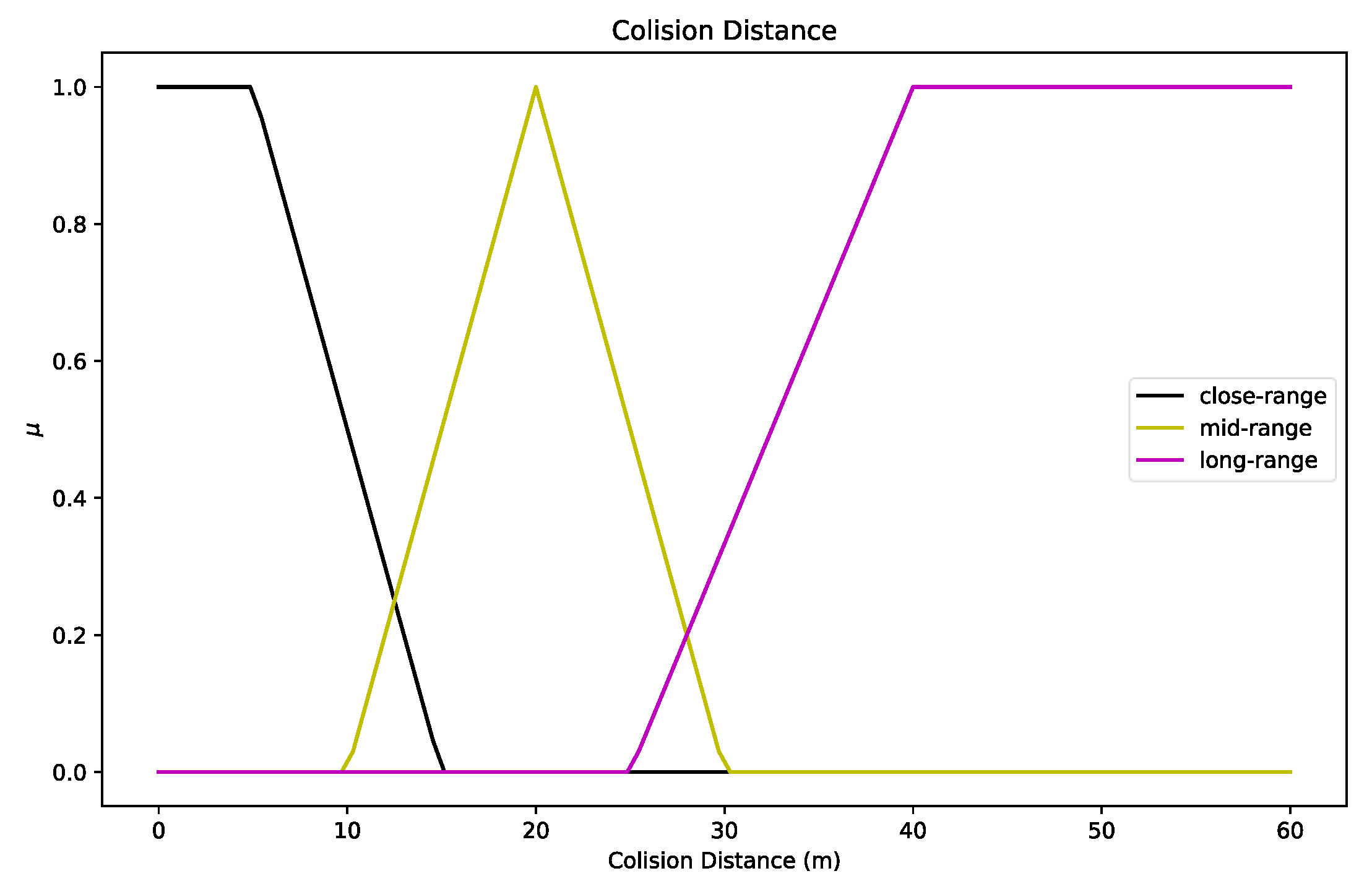
| 1 2 3 4 5 6 7 8 9 10 | distances = np.linspace(0,60,100) DistanceColision = UPAfs.fuzzy_universe('Collision Distance',distances,'continuous') DistanceColision.add_fuzzyset('close-range','trapmf',[0,0,5,15]) DistanceColision.add_fuzzyset('mid-range','trimf',[10,20,30]) DistanceColision.add_fuzzyset('long-range','trapmf',[25,40,60,60]) DistanceColision.view_fuzzy() ax = plt.gca() ax.set_xlabel('Collision Distance (m)') ax.set_ylabel("$\mu$") plt.show() |
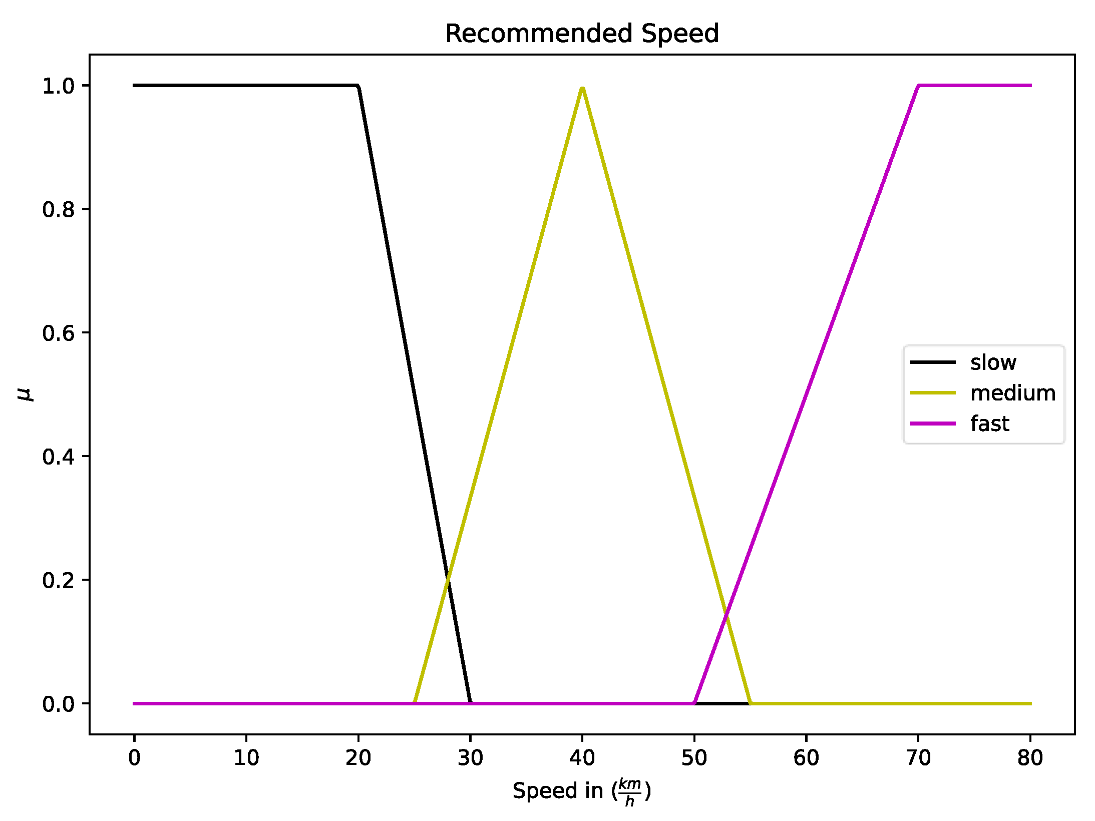
3.3. Fuzzy Inference System with Inference_System Class
- IF Collision Distance is short-range → Speed is slow
- IF Collision Distance is mid-range → Speed is medium
- IF Collision Distance is long-range → Speed is fast
| Code 3. Python code for defining inference system and its rules. | |
| 1 2 3 4 5 6 7 8 9 10 11 12 13 | Speed_Collision = UPAfs.inference_system("Speed based in Collision Distance") Speed_Collision.add_premise(DistanceColision) Speed_Collision.add_consequence(Speed) Speed_Collision.add_rule([['Collision Distance','close-range']],[],[['Recommended Speed','slow']]) Speed_Collision.add_rule([['Collision Distance','mid-range']],[],[['Recommended Speed','medium']]) Speed_Collision.add_rule([['Collision Distance','long-range']],[],[['Recommended Speed','fast']]) Speed_Collision.configure('Mamdani') Speed_Collision.build() Speed_Collision.surface_fuzzy_system([distances]) ax = plt.gca() ax.set_xlabel(r"Collision Distance (m)") ax.set_ylabel(r"Speed ($\frac{km}{h}$)") plt.show() |
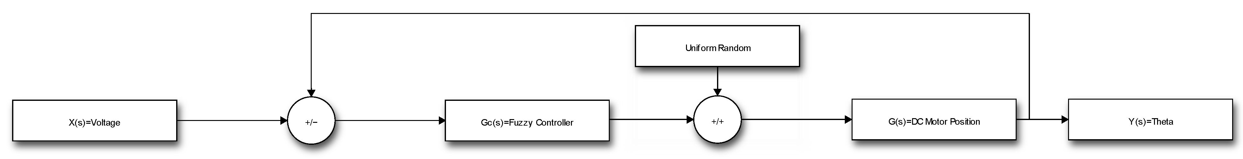
3.4. Fuzzy Controller with Fuzzy_Controller Class
| Code 4. Code for defining transfer function and its parameters in a DC motor. | |
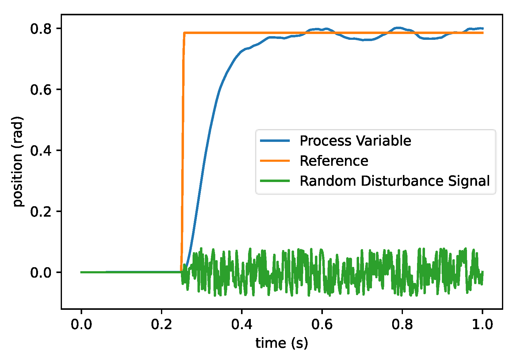
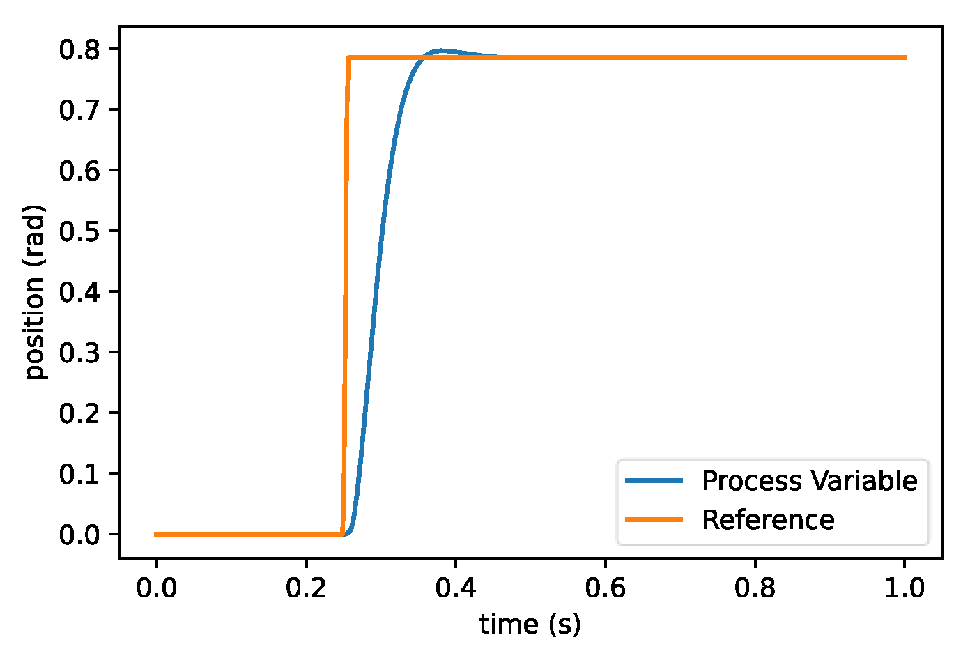
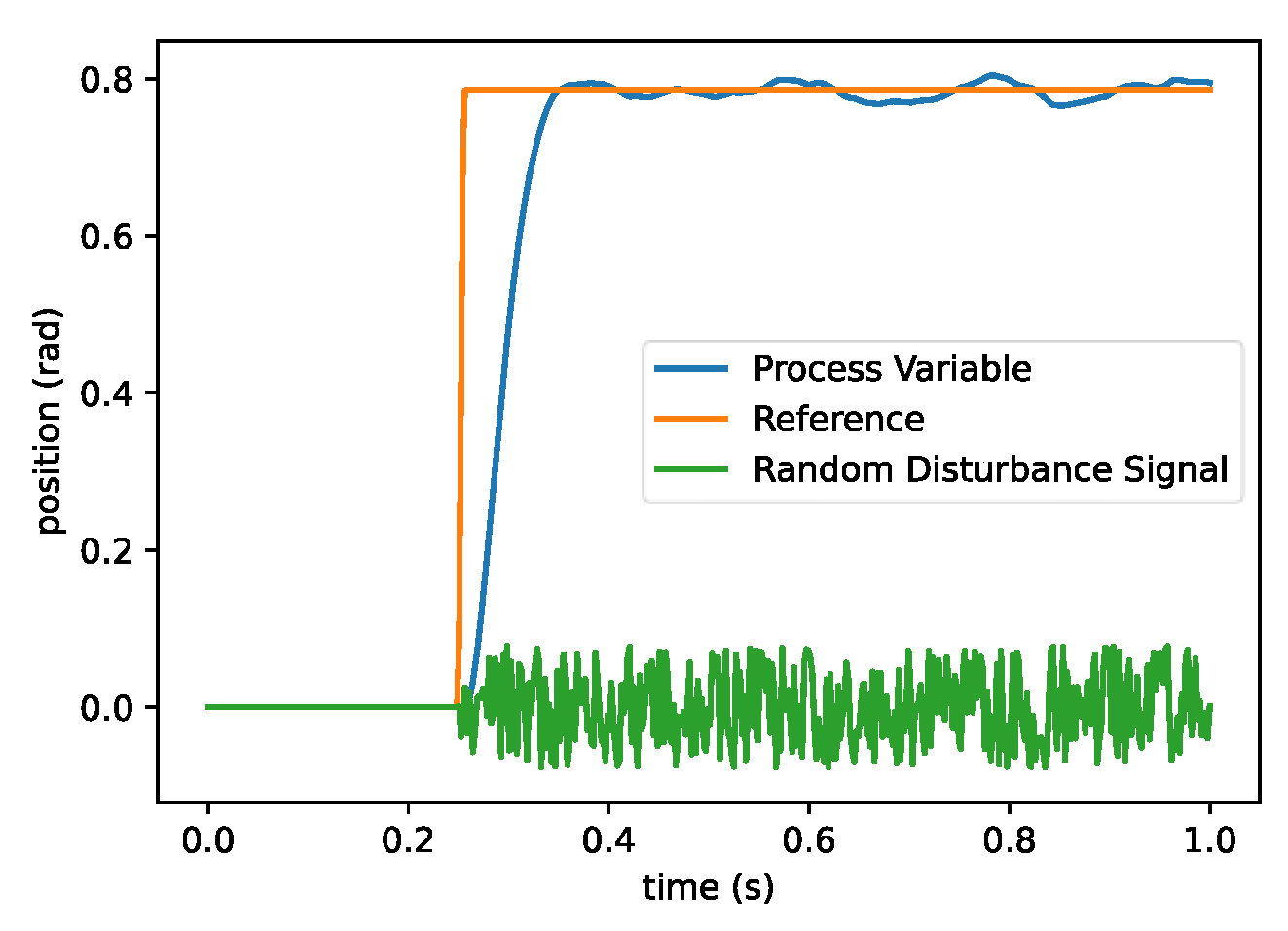
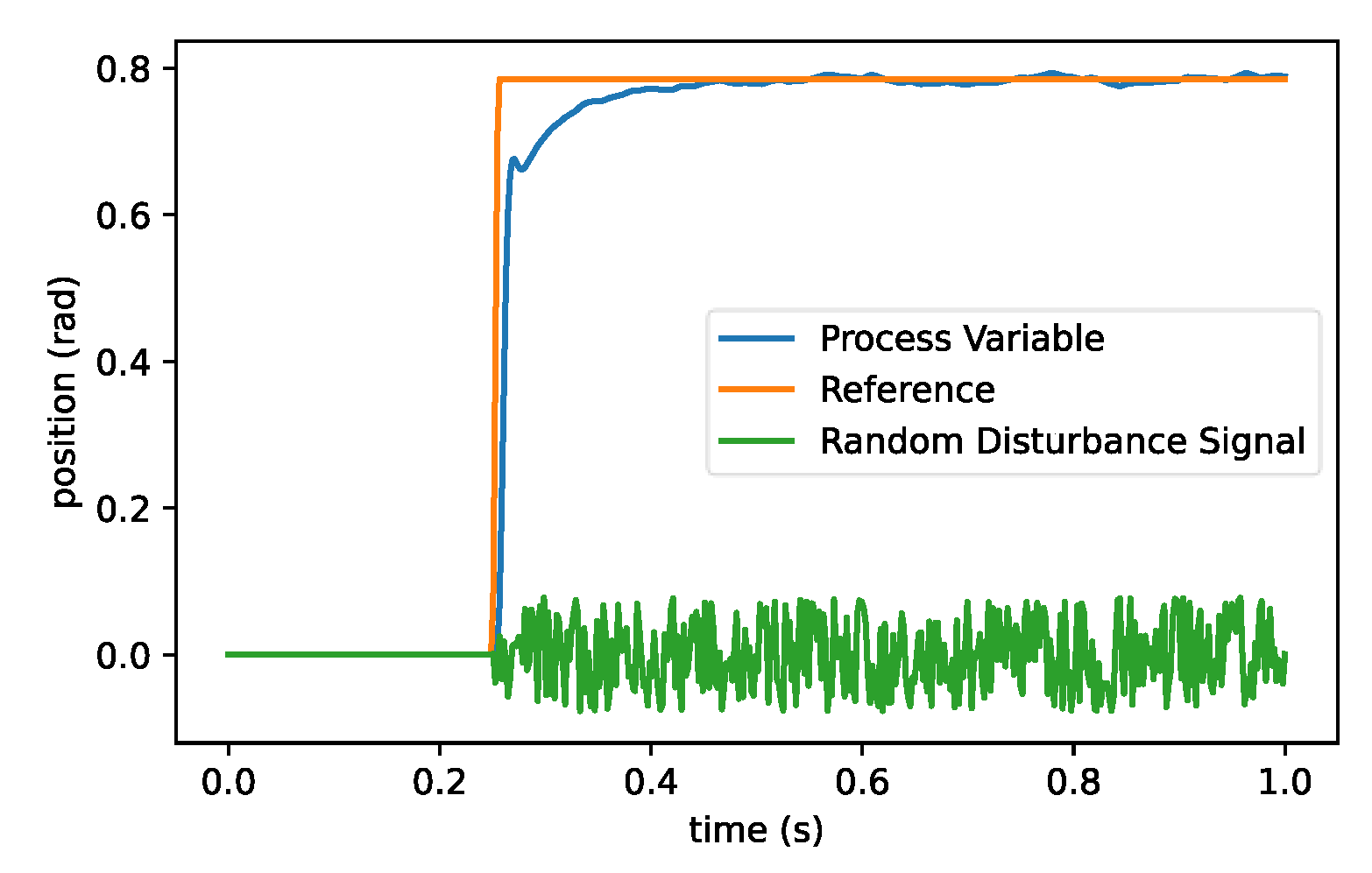
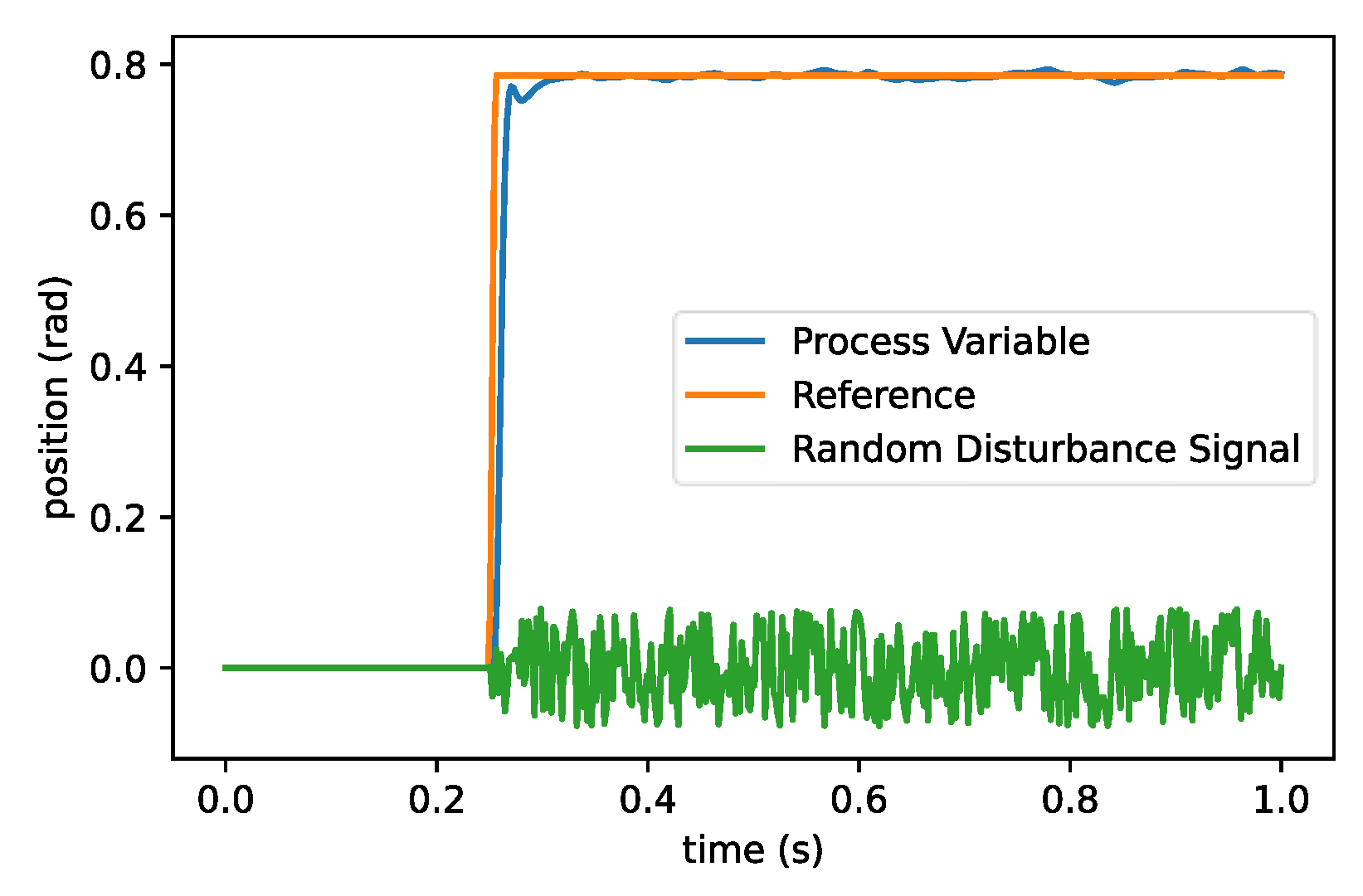
| 1 2 3 4 5 6 7 8 9 10 11 12 13 | J = 3.2284E-6 b = 3.5077E-6 K = 0.0274 R = 4 L = 2.75E-6 te = 1.0 ns = 500 T = np.linspace(0,te,ns) Input = np.array([(np.radians(45)*min((t-0.25)/0.005,1)) if t> 0.25 else 0 for t in T]) np.random.seed(0) Perturbation = np.array([np.random.uniform(-1,1)*i*0.1 for i in Input]) s = cn.TransferFunction.s TF = K/(s*((J*s+b)*(L*s+R)+K**2)) |
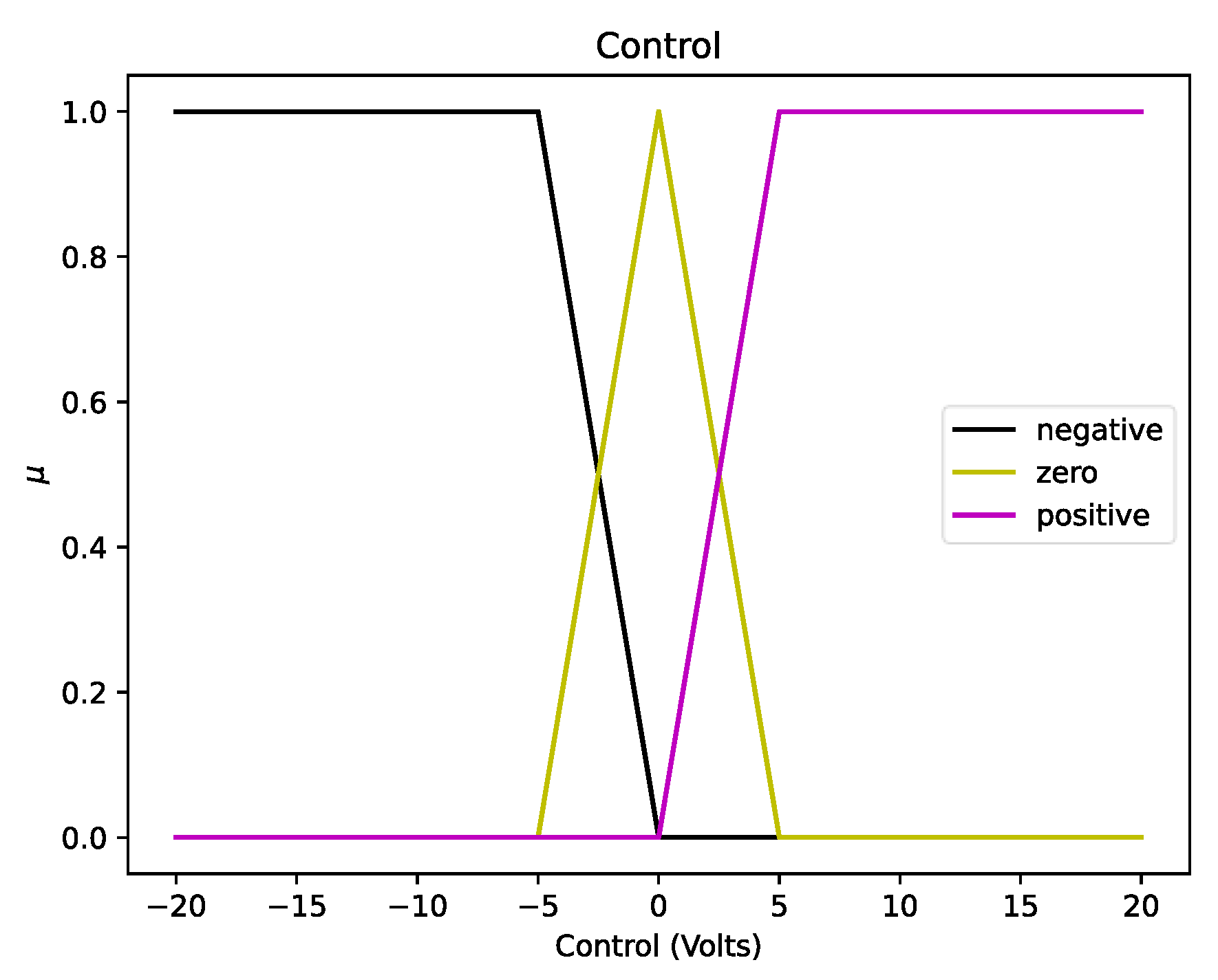
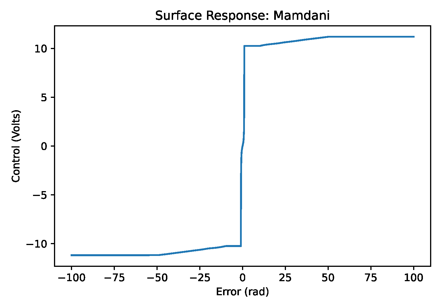
3.4.1. One-Input Mamdani Fuzzy Controller
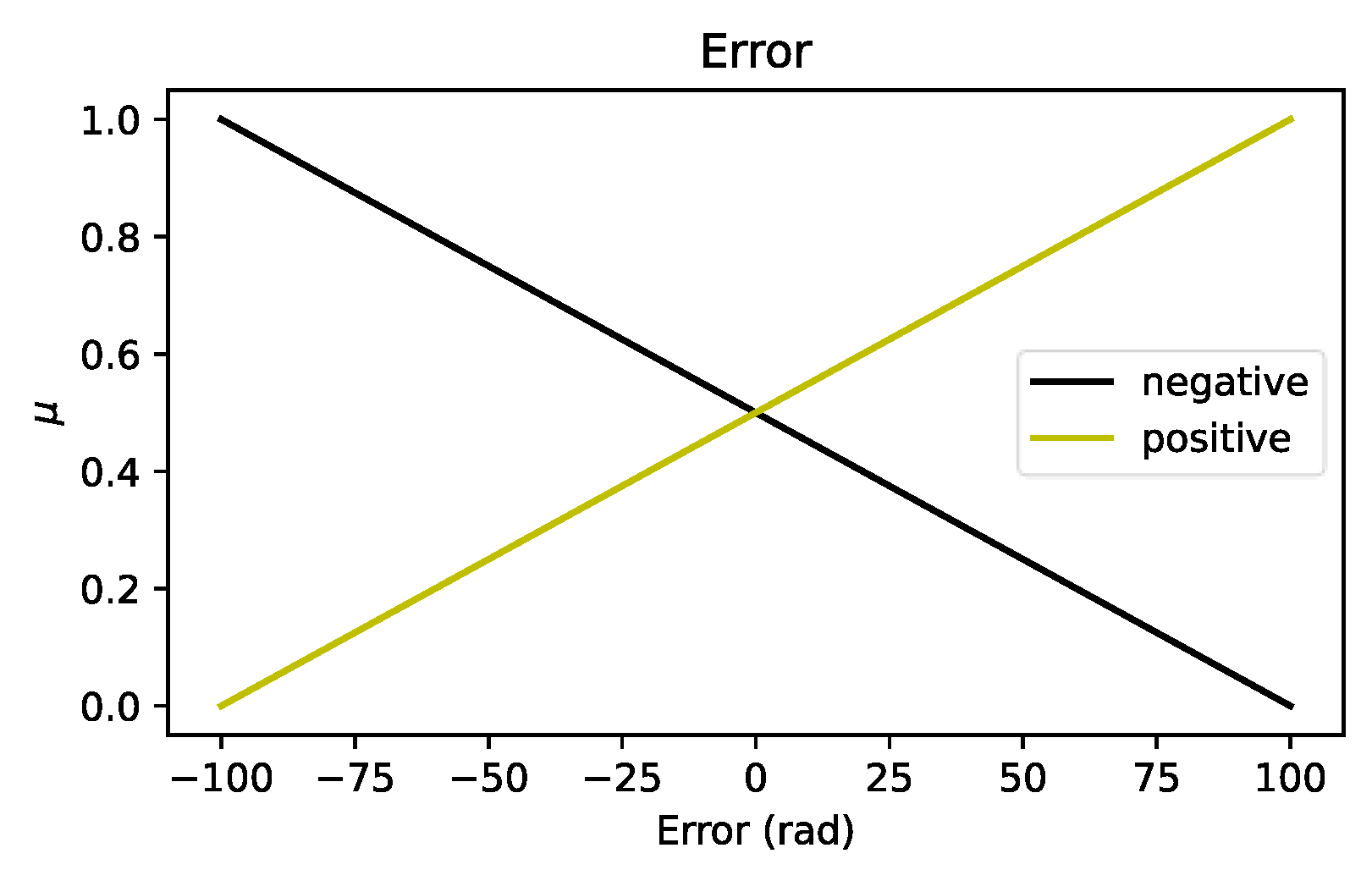
- IF Error is Negative → Control is Negative;
- IF Error is Zero → Control is Zero;
- IF Error is Positive → Control is Positive.
| Code 5. Python code for defining fuzzy controller with UPAFuzzySystems library. | |
| 1 2 3 4 | FuzzController = UPAfs.fuzzy_controller(Mamdani1,typec='Fuzzy1',tf=TF,DT = T[1]) FuzzController.build() FuzzControllerBlock = FuzzController.get_controller() FuzzSystemBlock = FuzzController.get_system() |
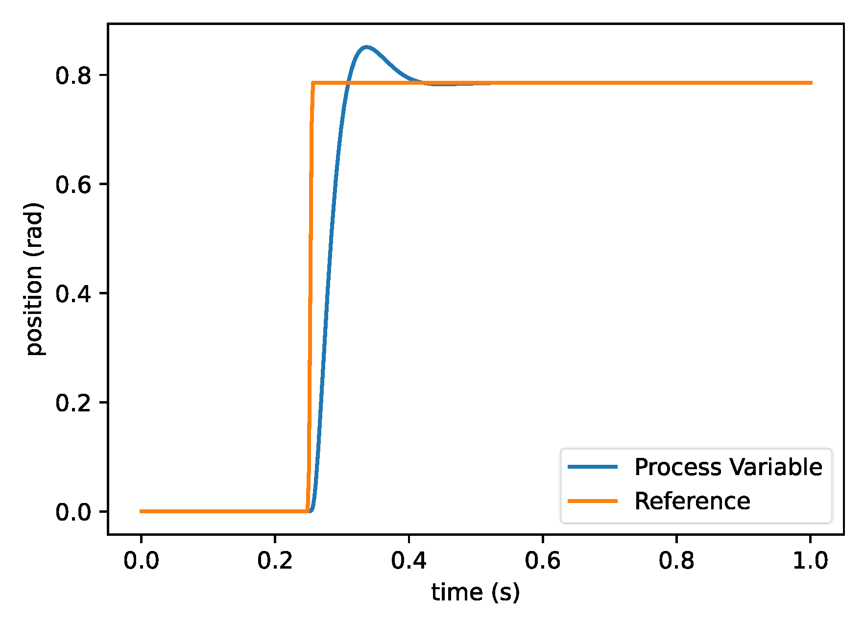
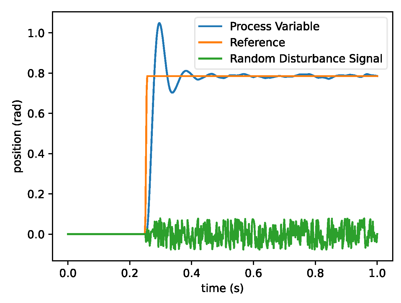
| Code 6. Python code for simulation of fuzzy controller and plotting results. | |
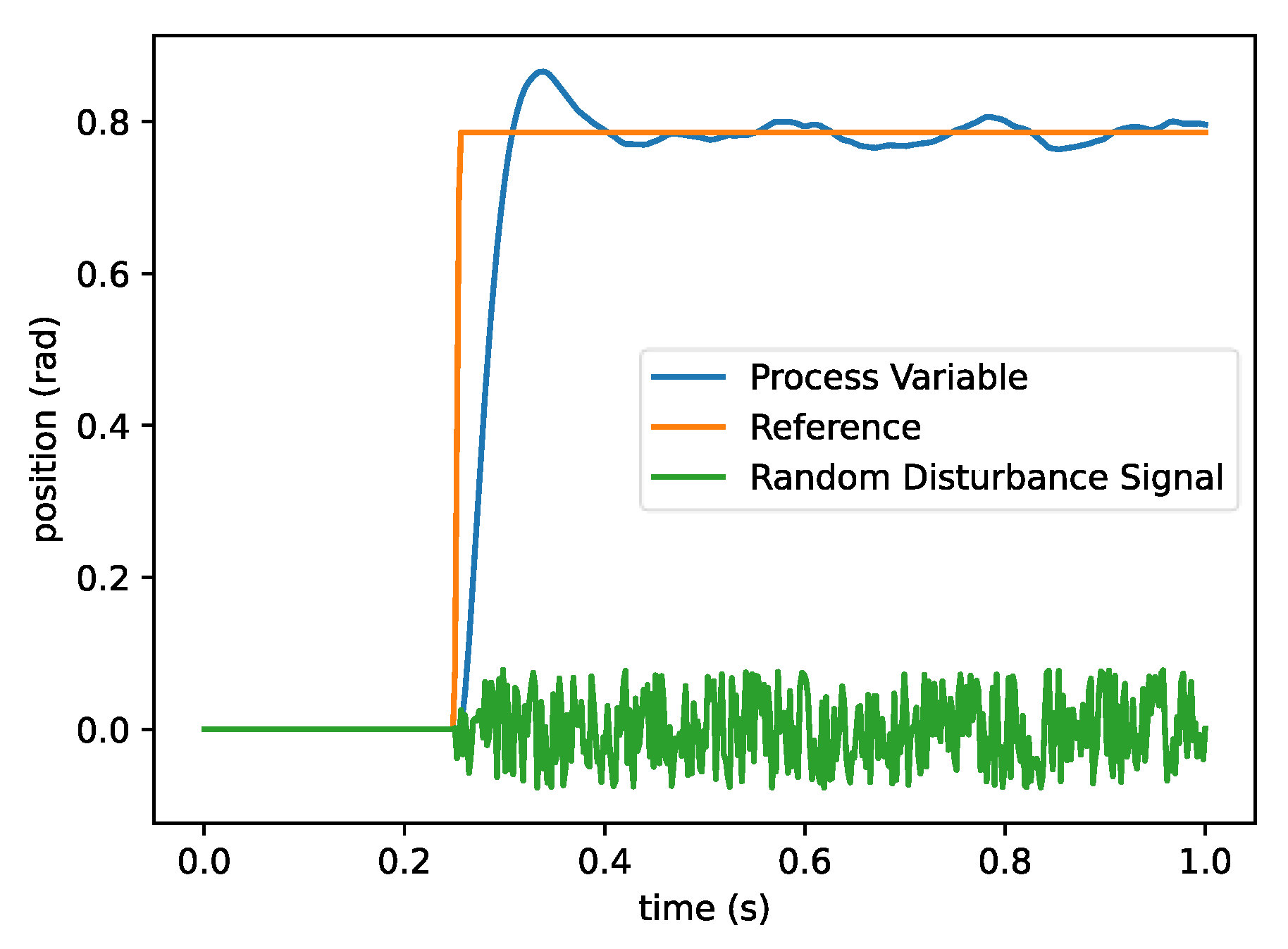
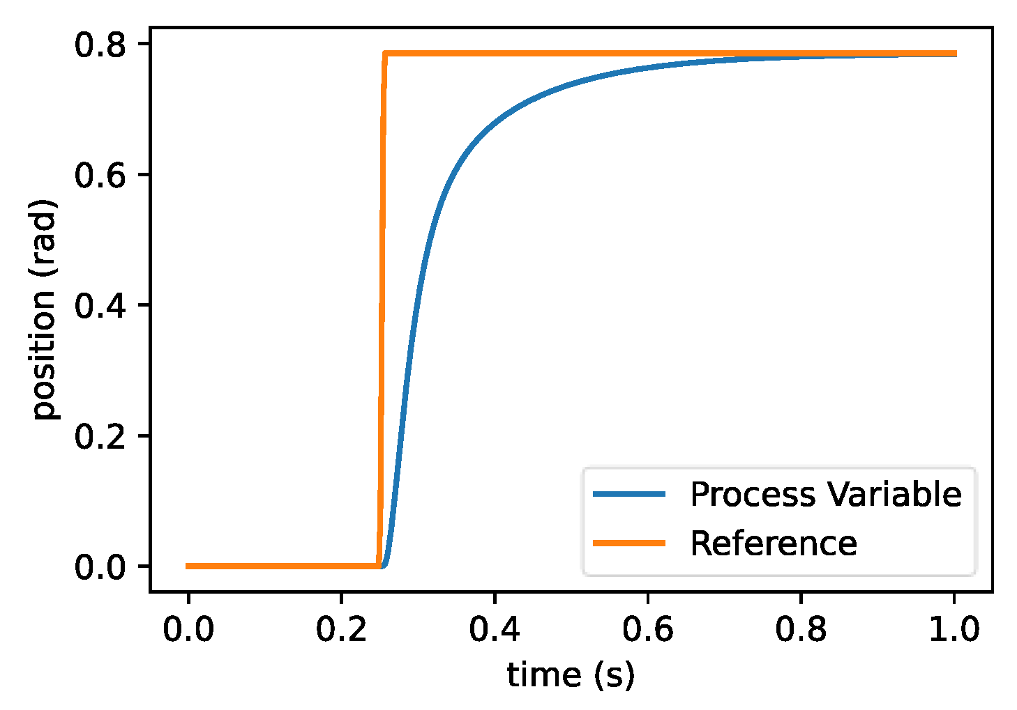
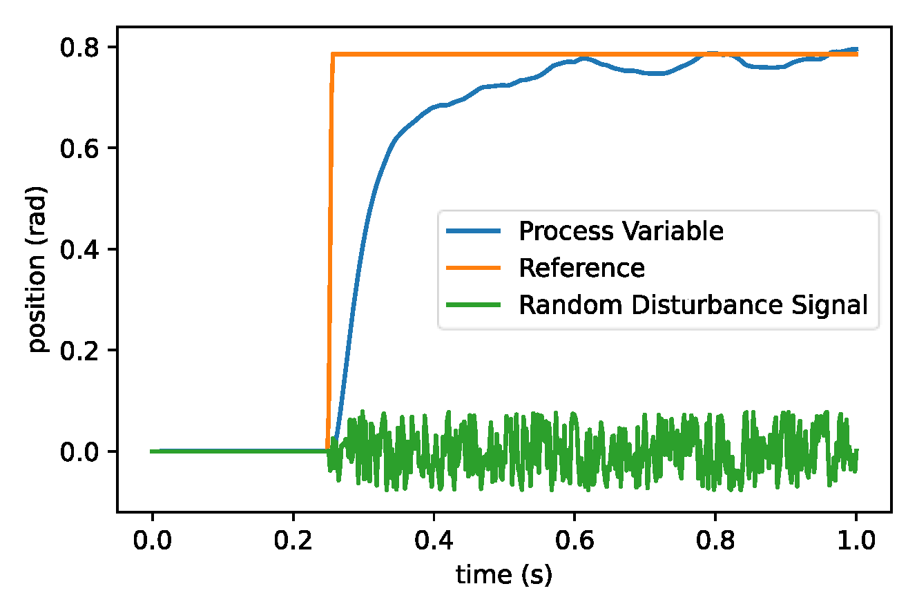
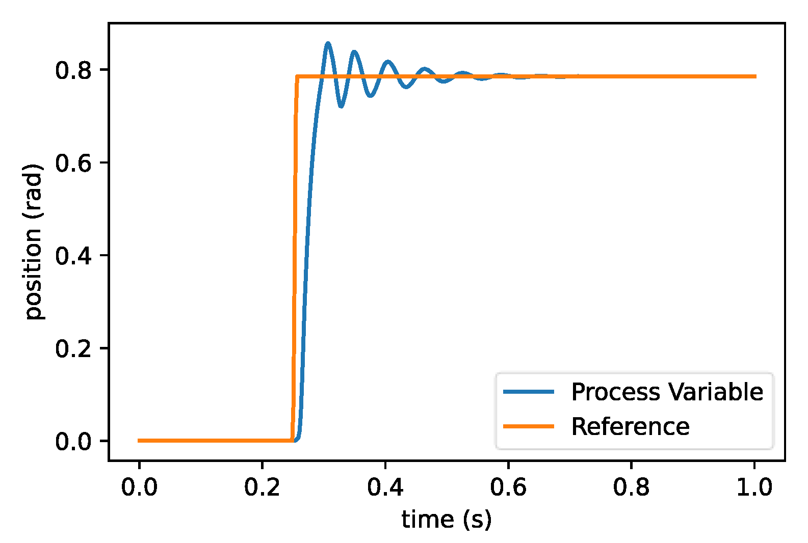
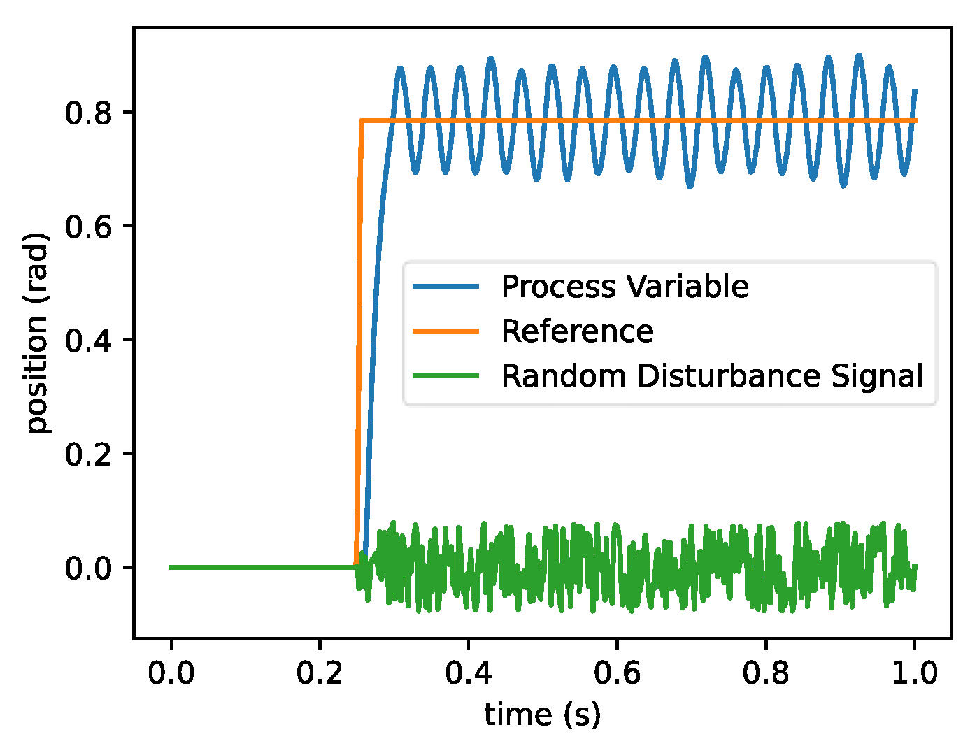
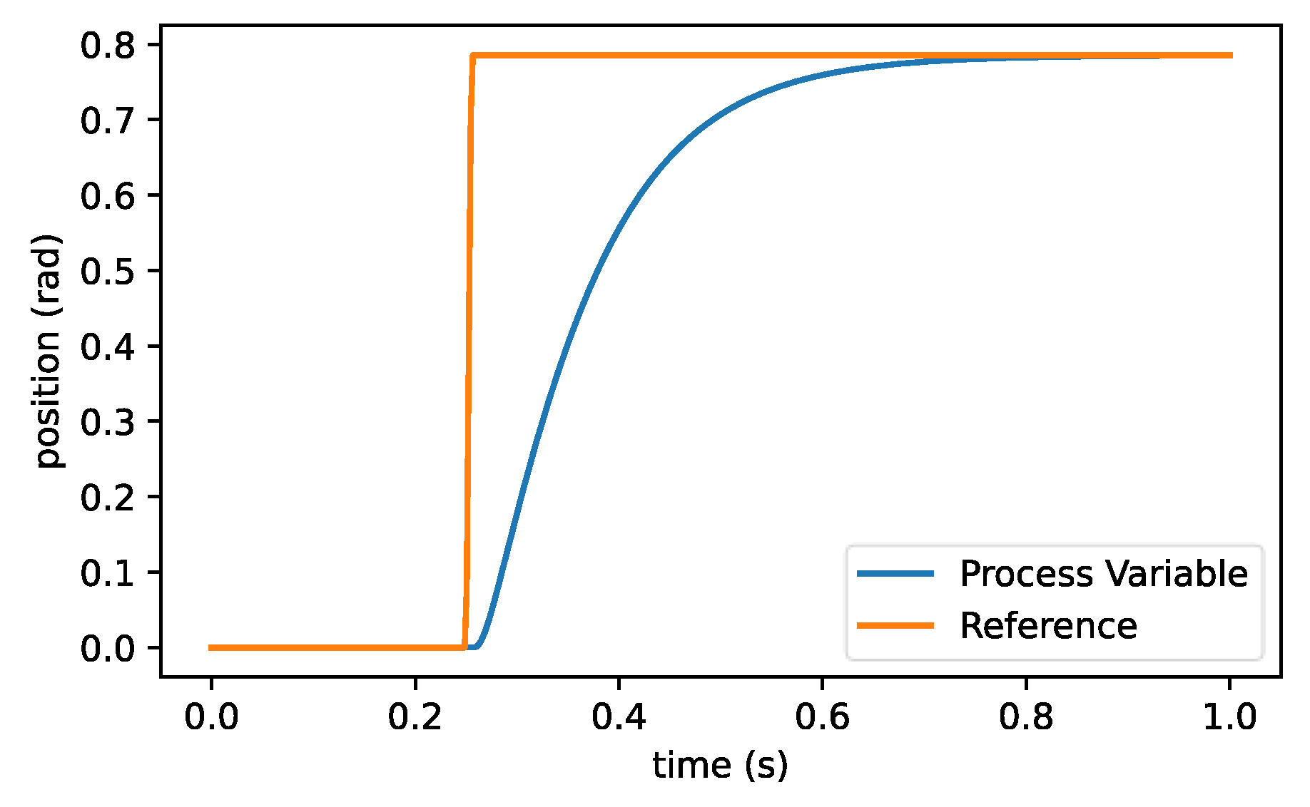
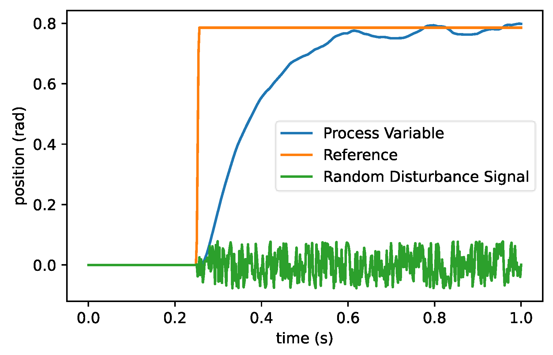
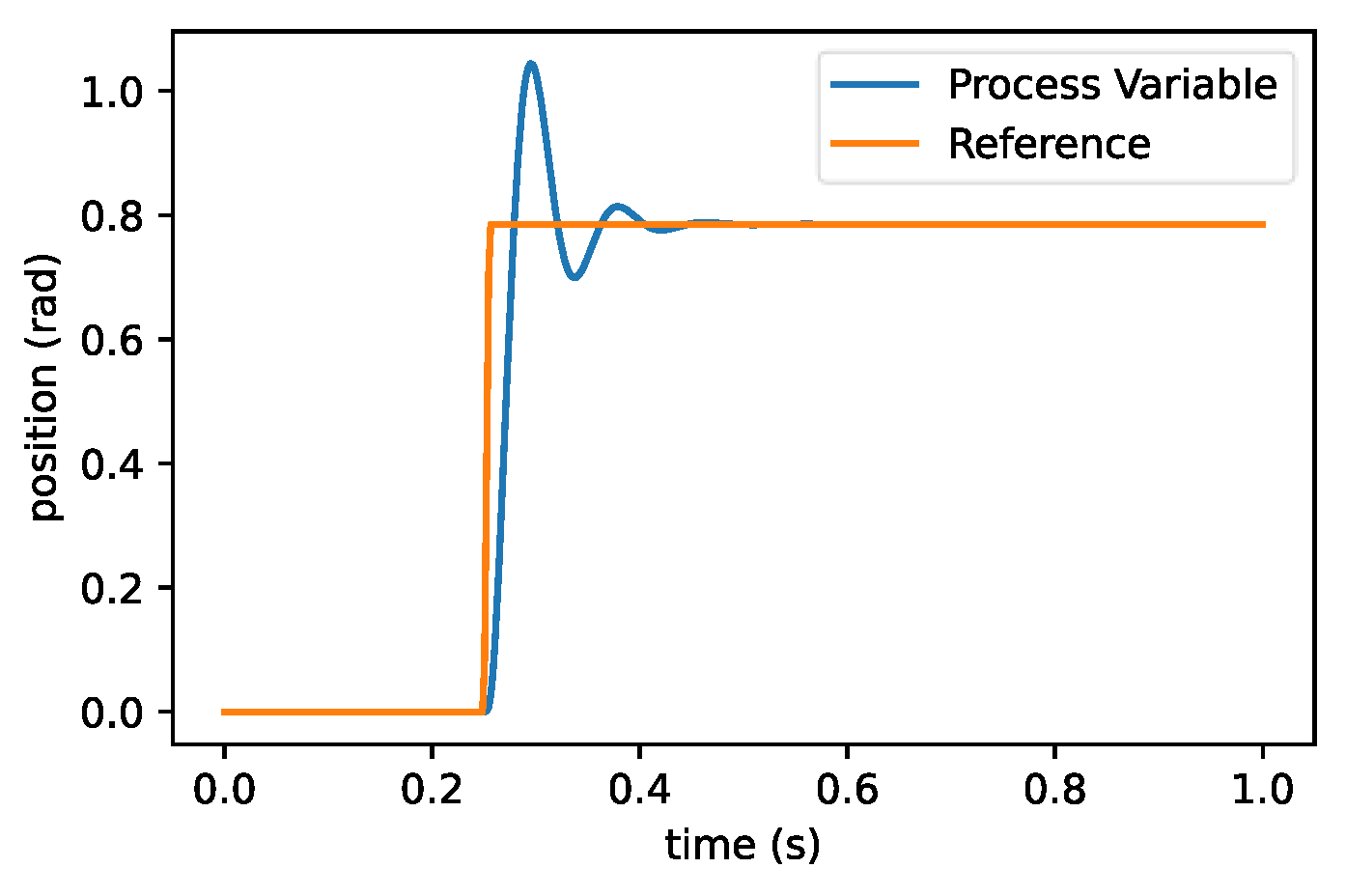
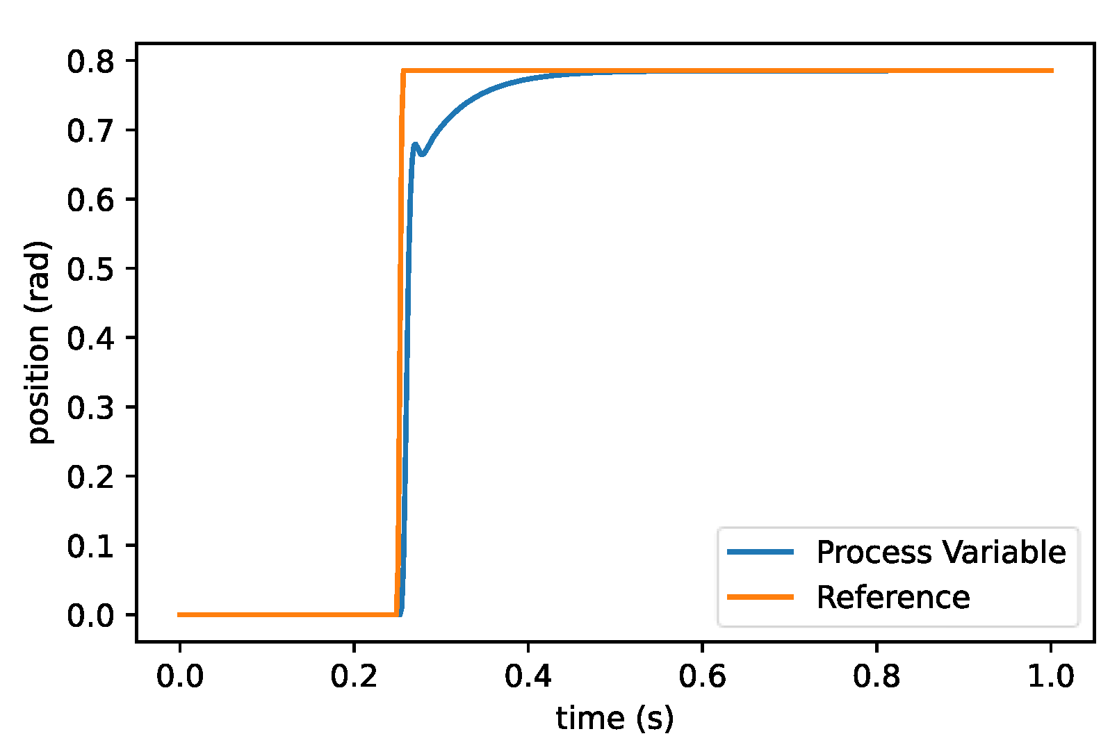
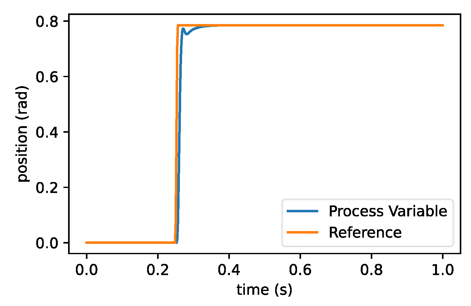
| 1 2 3 4 5 6 7 | T, Theta = cn.input_output_response(FuzzSystemBlock,T,Input,0) plt.plot(T,Theta,label='Process Variable') plt.plot(T,Input,label='Reference') plt.xlabel("time (s)") plt.ylabel("position (rad)") plt.legend() plt.show() |
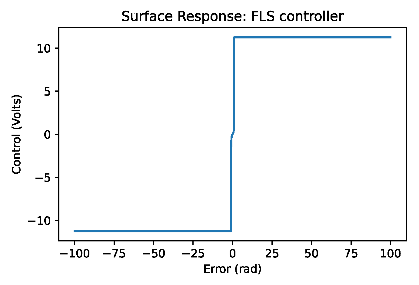
3.4.2. One-Input FLS Controller
| Code 7. Lines for defining one input FLS controller in the UPAFuzzySystems library. | |
| 1 2 3 4 5 6 7 8 | FLS1 = UPAfs.inference_system('FLS controller') FLS1.add_premise(Error_universe) FLS1.add_consequence(Control_universe) FLS1.add_rule([['Error','negative']],[],[['Control','negative']]) FLS1.add_rule([['Error','zero']],[],[['Control','zero']]) FLS1.add_rule([['Error','positive']],[],[['Control','positive']]) FLS1.configure('FLSmidth') FLS1.build() |
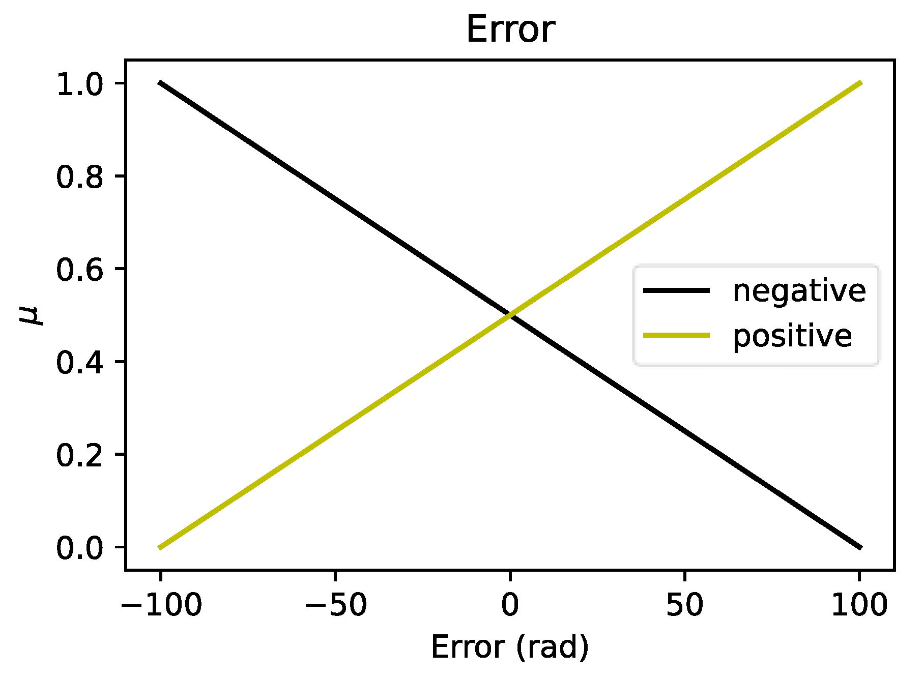
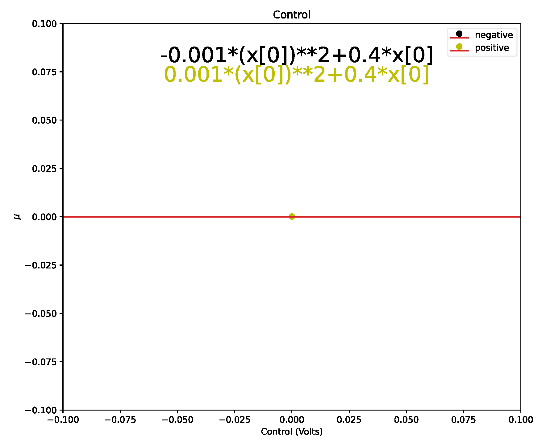
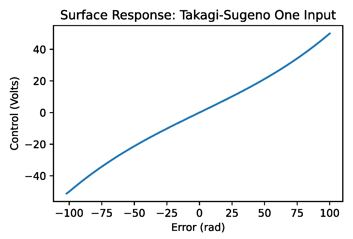
3.4.3. One Input Takagi–Sugeno Controller
| Code 8. Python code for the fuzzy universe and inference system for the one-input Takagi–Sugeno controller. | |
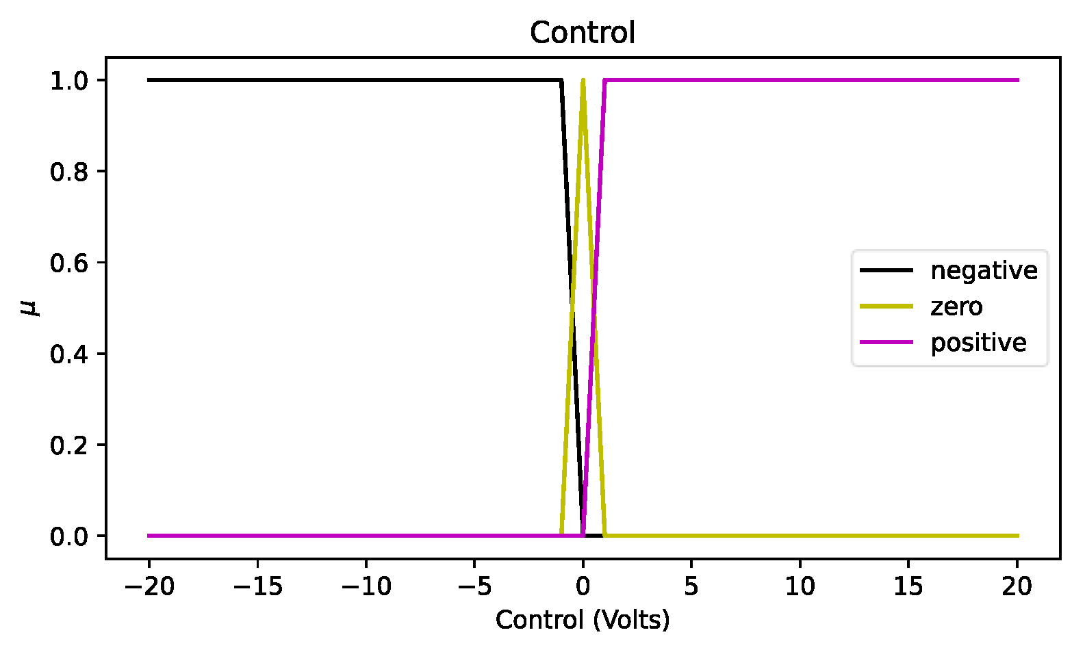
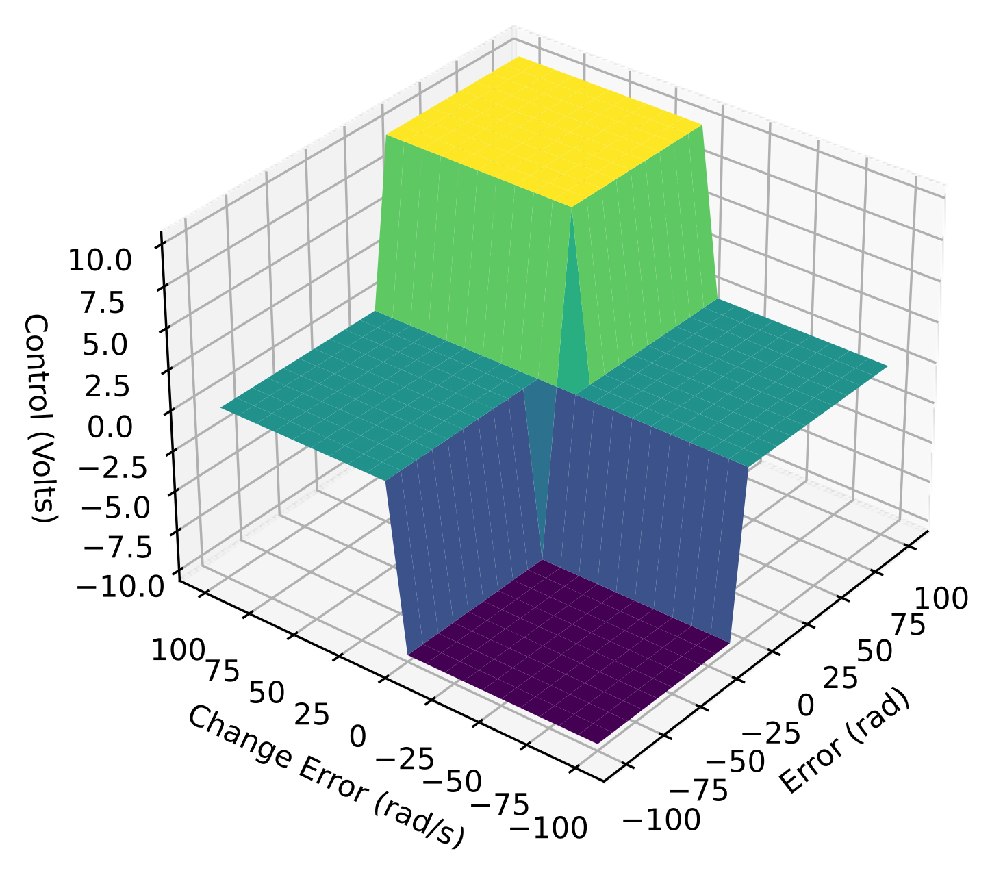
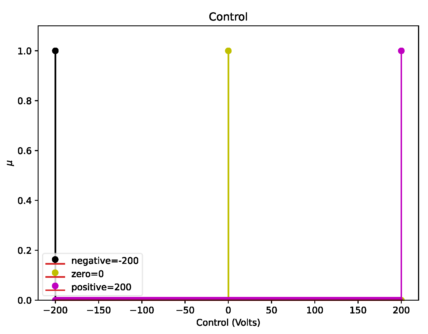
| 1 2 3 4 5 6 7 8 9 10 11 12 13 14 15 16 17 18 19 20 21 22 23 24 25 26 27 | Error_universe = UPAfs.fuzzy_universe('Error', np.arange(-100,101,1), 'continuous') Error_universe.add_fuzzyset('negative','trimf',[-200,-100,100]) Error_universe.add_fuzzyset('positive','trimf',[-100,100,200]) Error_universe.view_fuzzy() ax = plt.gca() ax.set_xlabel("Error (rad)") ax.set_ylabel("$\mu$") plt.show() Control_universe = UPAfs.fuzzy_universe('Control', np.arange(-20,22,2), 'continuous') Control_universe.add_fuzzyset('negative','eq','-0.001*(x[0])**2+0.4*x[0]') Control_universe.add_fuzzyset('positive','eq','0.001*(x[0])**2+0.4*x[0]') Control_universe.view_fuzzy() ax = plt.gca() ax.set_xlabel("Control (Volts)") ax.set_ylabel("$\mu$") plt.show() TSG1 = UPAfs.inference_system('Takagi-Sugeno One Input') TSG1.add_premise(Error_universe) TSG1.add_consequence(Control_universe) TSG1.add_rule([['Error','negative']],[],[['Control','negative']]) TSG1.add_rule([['Error','positive']],[],[['Control','positive']]) TSG1.configure('Sugeno') TSG1.build() |
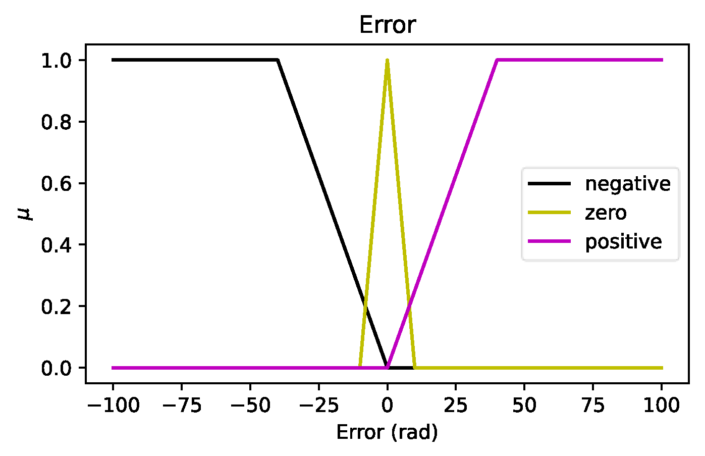
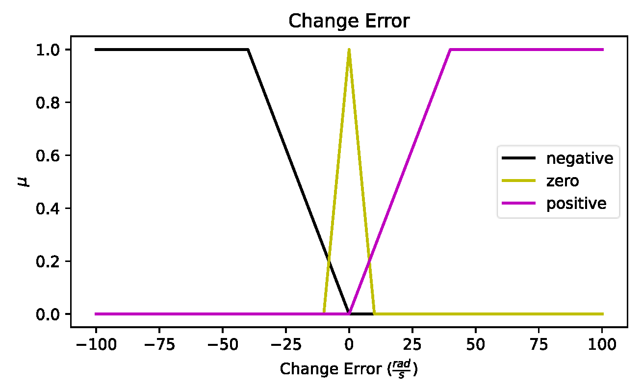
3.4.4. Two-Input Mamdani Controller
- If error is Neg and change error is Neg then control is Neg;
- If error is Neg and change error is Zero then control is Neg;
- If error is Zero and change error is Neg then control is Zero;
- If error is Neg and change error is Pos then control is Zero;
- If error is Zero and change error is Zero then control is Zero;
- If error is Zero and change error is Pos then control is Zero;
- If error is Pos and change error is Neg then control is Zero;
- If error is Pos and change error is Zero then control is Pos;
- If error is Pos and change error is Pos then control is Pos.
| Code 9. Python code with rules for a two-input Mamdani controller using the UPAFuzzySystems library. | |
| 1 2 3 4 5 6 7 8 9 10 11 12 13 14 15 | Mamdani2 = UPAfs.inference_system('Mamdani') Mamdani2.add_premise(Error_universe) Mamdani2.add_premise(ChError_universe) Mamdani2.add_consequence(Control_universe) Mamdani2.add_rule([['Error','negative'],['Change Error','negative']],['and'],[['Control','negative']]) Mamdani2.add_rule([['Error','negative'],['Change Error','zero']],['and'],[['Control','negative']]) Mamdani2.add_rule([['Error','zero'],['Change Error','negative']],['and'],[['Control','zero']]) Mamdani2.add_rule([['Error','negative'],['Change Error','positive']],['and'],[['Control','zero']]) Mamdani2.add_rule([['Error','zero'],['Change Error','zero']],['and'],[['Control','zero']]) Mamdani2.add_rule([['Error','positive'],['Change Error','negative']],['and'],[['Control','zero']]) Mamdani2.add_rule([['Error','zero'],['Change Error','positive']],['and'],[['Control','zero']]) Mamdani2.add_rule([['Error','positive'],['Change Error','zero']],['and'],[['Control','positive']]) Mamdani2.add_rule([['Error','positive'],['Change Error','positive']],['and'],[['Control','positive']]) Mamdani2.configure('Mamdani') Mamdani2.build() |
| Code 10. Python code for configuring two-input Mamdani controller using the UPAFuzzySystems library. | |
| 1 2 3 4 | MamdaniController = UPAfs.fuzzy_controller(Mamdani2,typec='Fuzzy2',tf=TF,DT = T[1]) MamdaniController.build() MamdaniControllerBlock = MamdaniController.get_controller() MamdaniSystemBlock = MamdaniController.get_system() |
3.4.5. Two-Input FLS Controller
3.4.6. Two Inputs Takagi–Sugeno Controller
| Code 11. Code for defining the inference system and the fuzzy universe for the two-input Takagi–Sugeno controller. | |
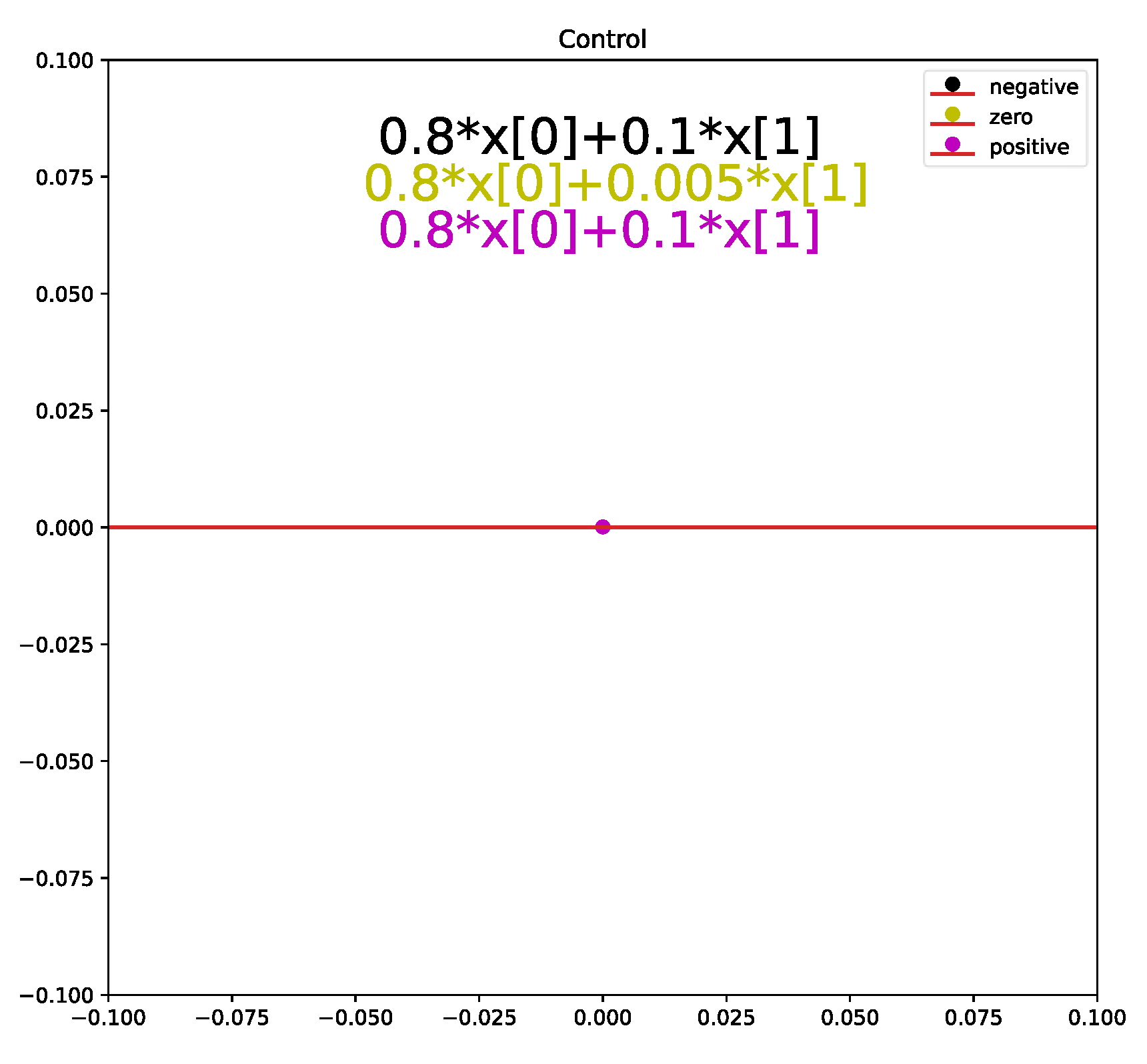
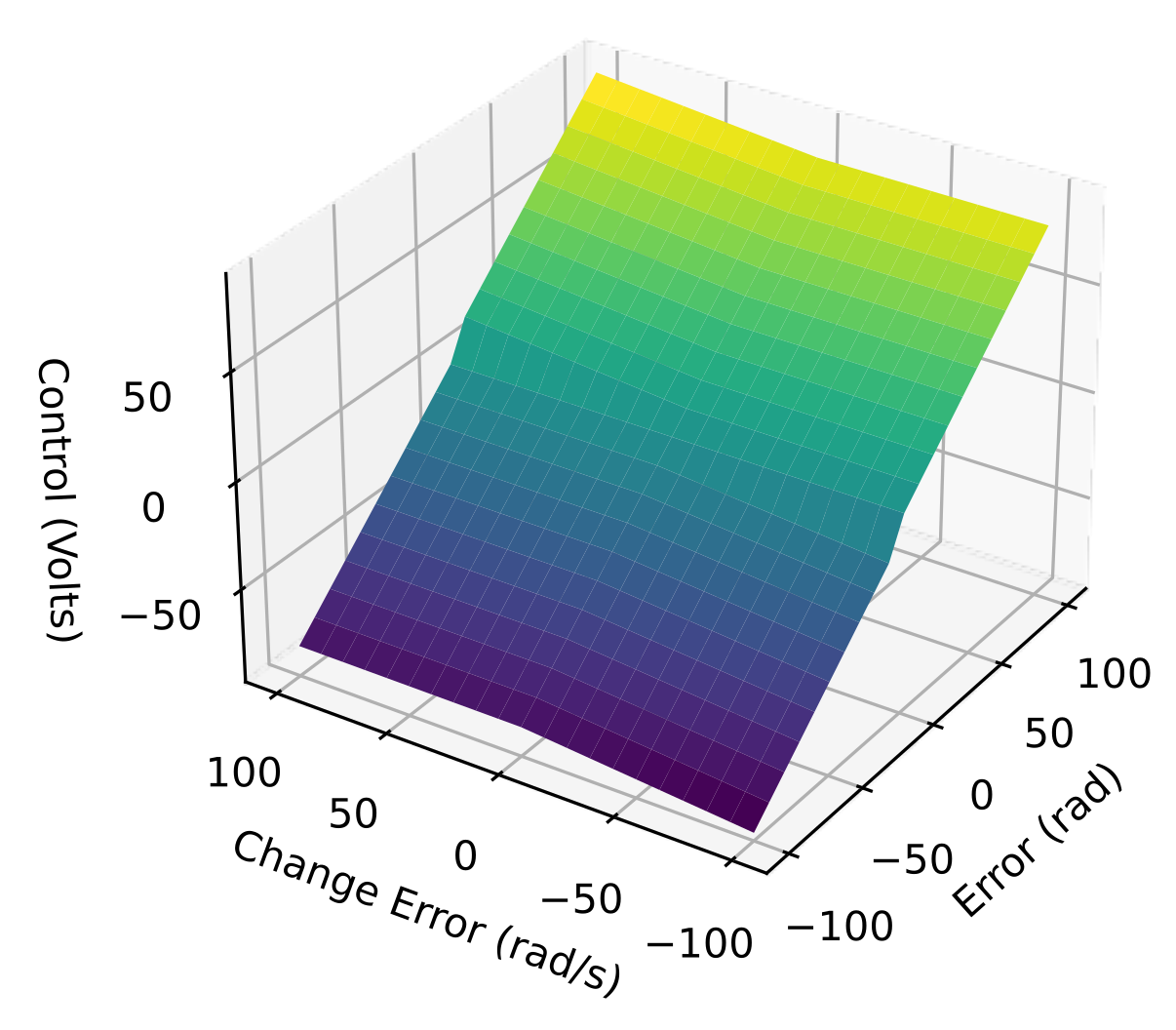
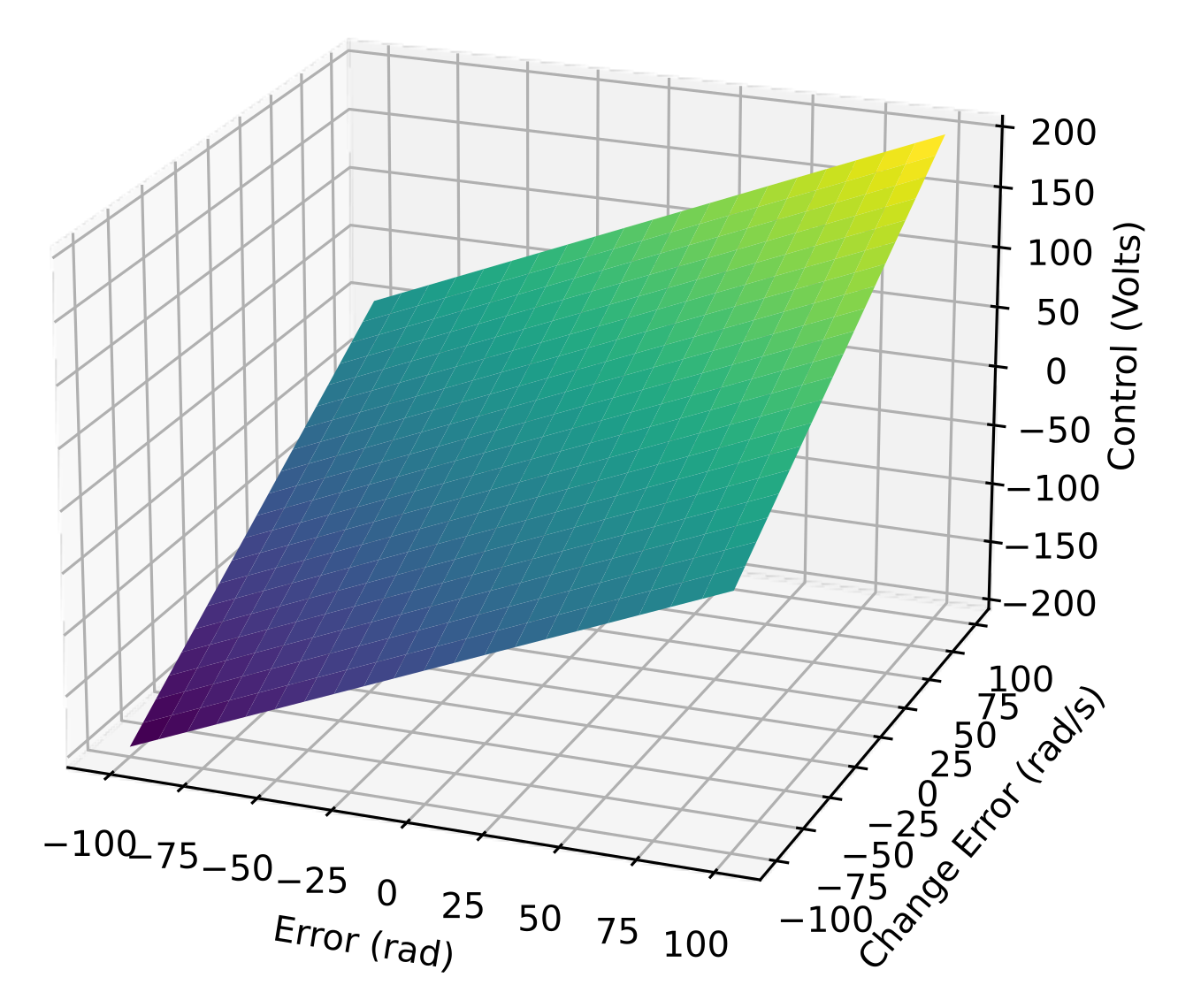
| 1 2 3 4 5 6 7 8 9 10 11 12 13 14 15 16 17 18 19 20 21 22 23 24 25 26 27 28 29 30 31 32 33 34 35 36 | Error_universe = UPAfs.fuzzy_universe('Error', np.arange(-100,101,1), 'continuous') Error_universe.add_fuzzyset('negative','trapmf',[-100,-100,-40,0]) Error_universe.add_fuzzyset('zero','trimf',[-10,0,10]) Error_universe.add_fuzzyset('positive','trapmf',[0,40,100,100]) Error_universe.view_fuzzy() ChError_universe = UPAfs.fuzzy_universe('Change Error', np.arange(-100,101,1), 'continuous') ChError_universe.add_fuzzyset('negative','trapmf',[-100,-100,-40,0]) ChError_universe.add_fuzzyset('zero','trimf',[-10,0,10]) ChError_universe.add_fuzzyset('positive','trapmf',[0,40,100,100]) ChError_universe.view_fuzzy() Control_universe = UPAfs.fuzzy_universe('Control', np.arange(-20,22,2), 'continuous') Control_universe.add_fuzzyset('negative','eq','0.8*x[0]+0.1*x[1]') Control_universe.add_fuzzyset('zero','eq','0.8*x[0]+0.005*x[1]') Control_universe.add_fuzzyset('positive','eq','0.8*x[0]+0.1*x[1]') Control_universe.view_fuzzy() TSG2 = UPAfs.inference_system('Takagi-Sugeno Two Inputs') TSG2.add_premise(Error_universe) TSG2.add_premise(ChError_universe) TSG2.add_consequence(Control_universe) TSG2.add_rule([['Error','negative'],['Change Error','negative']],['and'],[['Control','negative']]) TSG2.add_rule([['Error','negative'],['Change Error','zero']],['and'],[['Control','negative']]) TSG2.add_rule([['Error','zero'],['Change Error','negative']],['and'],[['Control','zero']]) TSG2.add_rule([['Error','negative'],['Change Error','positive']],['and'],[['Control','zero']]) TSG2.add_rule([['Error','zero'],['Change Error','zero']],['and'],[['Control','zero']]) TSG2.add_rule([['Error','positive'],['Change Error','negative']],['and'],[['Control','zero']]) TSG2.add_rule([['Error','zero'],['Change Error','positive']],['and'],[['Control','zero']]) TSG2.add_rule([['Error','positive'],['Change Error','zero']],['and'],[['Control','positive']]) TSG2.add_rule([['Error','positive'],['Change Error','positive']],['and'],[['Control','positive']]) TSG2.configure('Sugeno') TSG2.build() |
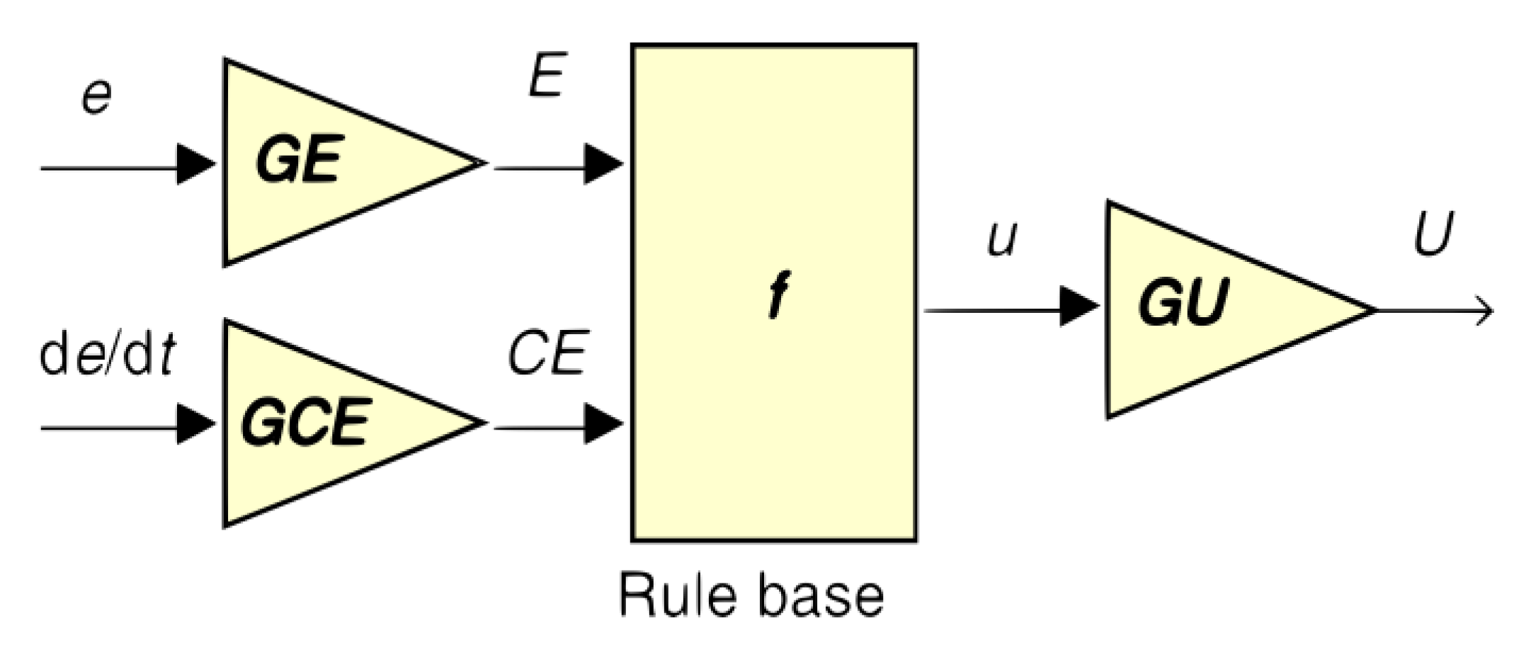
3.5. P, PD, and PID Fuzzy Controllers
3.5.1. Linear P Fuzzy Controller
| Code 12. Code for defining the one-input fuzzy linear system used in the linear P fuzzy controller. | |
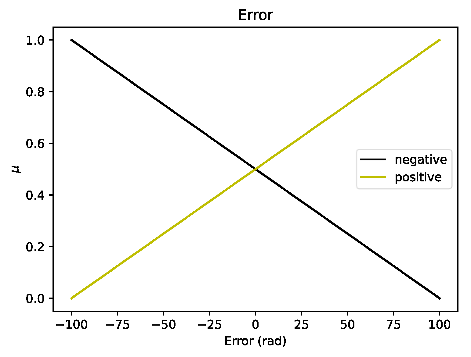
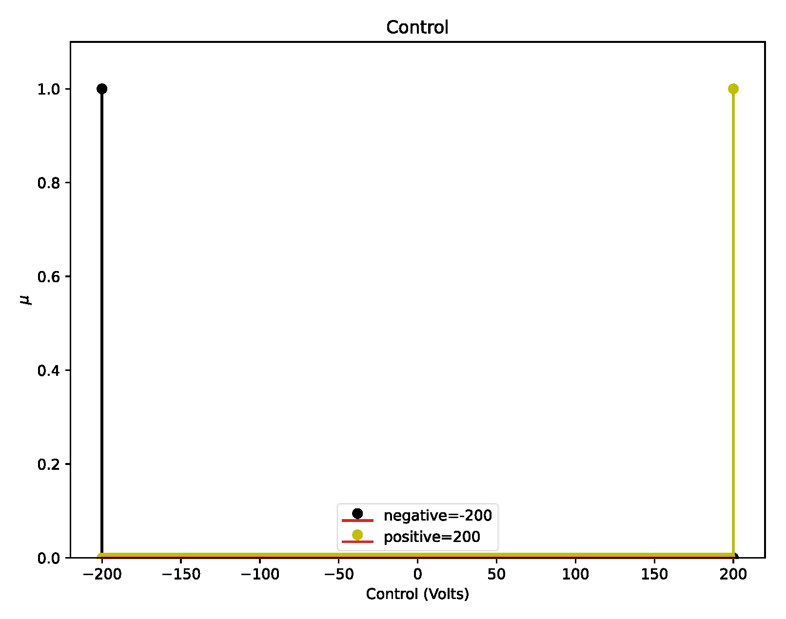
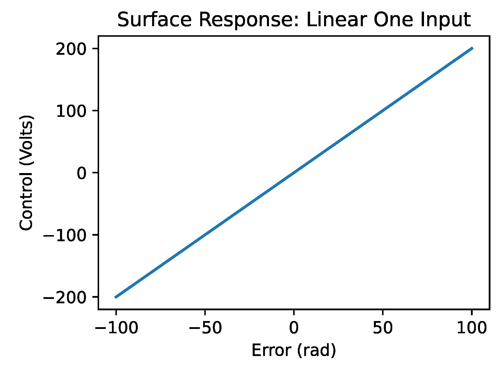
| 1 2 3 4 5 6 7 8 9 10 11 12 13 14 15 16 17 18 19 20 21 22 23 24 25 26 27 | Error_universe = UPAfs.fuzzy_universe('Error', np.arange(-100,101,1), 'continuous') Error_universe.add_fuzzyset('negative','trimf',[-200,-100,100]) Error_universe.add_fuzzyset('positive','trimf',[-100,100,200]) Error_universe.view_fuzzy() ax = plt.gca() ax.set_xlabel("Error (rad)") ax.set_ylabel("$\mu$") plt.show() Control_universe = UPAfs.fuzzy_universe('Control', np.arange(-200,202,2), 'continuous') Control_universe.add_fuzzyset(‘negative’,’ eq’, ‘-200’) Control_universe.add_fuzzyset('positive','eq','200') Control_universe.view_fuzzy() ax = plt.gca() ax.set_xlabel("Control (Volts)") ax.set_ylabel("$\mu$") plt.show() LinearP = UPAfs.inference_system('Linear One Input') LinearP.add_premise(Error_universe) LinearP.add_consequence(Control_universe) LinearP.add_rule([['Error','negative']],[],[['Control','negative']]) LinearP.add_rule([['Error','positive']],[],[['Control','positive']]) LinearP.configure('Linear') LinearP.build() |
| Code 13. Python code for configuring the linear fuzzy proportional controller with the UPAFuzzySystems library. | |
| 1 2 3 4 | LinearPFuzzController = UPAfs.fuzzy_controller(LinearP,typec='P',tf=TF,DT = T[1], GE=15.91545709, GU=0.094248) LinearPFuzzController.build() LinearPFuzzControllerBlock = LinearPFuzzController.get_controller() LinearPFuzzSystemBlock = LinearPFuzzController.get_system() |
3.5.2. Linear PD Fuzzy Controller
| Code 14. Code for defining the two-input fuzzy linear system with UPAFuzzySystems library. | |
| 1 2 3 4 5 6 7 8 9 10 11 12 13 14 15 16 17 18 19 20 21 22 23 24 25 26 27 28 29 30 31 32 33 34 35 36 37 38 39 40 41 | Error_universe = UPAfs.fuzzy_universe('Error', np.arange(-100,101,1), 'continuous') Error_universe.add_fuzzyset('negative','trimf',[-200,-100,100]) Error_universe.add_fuzzyset('positive','trimf',[-100,100,200]) Error_universe.view_fuzzy() ax = plt.gca() ax.set_xlabel("Error (rad)") ax.set_ylabel("$\mu$") plt.show() ChError_universe = UPAfs.fuzzy_universe('Change Error', np.arange(-100,101,1), 'continuous') ChError_universe.add_fuzzyset('negative','trimf',[-200,-100,100]) ChError_universe.add_fuzzyset('positive','trimf',[-100,100,200]) ChError_universe.view_fuzzy() ax = plt.gca() ax.set_xlabel(r"Change Error ($\frac{rad}{s}$)") ax.set_ylabel("$\mu$") plt.show() Control_universe = UPAfs.fuzzy_universe('Control', np.arange(-200,202,2), 'continuous') Control_universe.add_fuzzyset(‘negative’,’ eq’, ‘-200’) Control_universe.add_fuzzyset(‘zero’, ‘eq’, ‘0’) Control_universe.add_fuzzyset('positive','eq','200') Control_universe.view_fuzzy() ax = plt.gca() ax.set_xlabel("Control (Volts)") ax.set_ylabel("$\mu$") plt.show() Linear = UPAfs.inference_system('Linear') Linear.add_premise(Error_universe) Linear.add_premise(ChError_universe) Linear.add_consequence(Control_universe) Linear.add_rule([['Error','negative'],['Change Error','negative']],['and'],[['Control','negative']]) Linear.add_rule([['Error','negative'],['Change Error','positive']],['and'],[['Control','zero']]) Linear.add_rule([['Error','positive'],['Change Error','negative']],['and'],[['Control','zero']]) Linear.add_rule([['Error','positive'],['Change Error','positive']],['and'],[['Control','positive']]) Linear.configure('Linear') Linear.build() |
| Code 15. Python code for configuring the PD fuzzy controller in the UPAFuzzySystems library. | |
| 1 2 3 4 | LinearPDFuzzController = UPAfs.fuzzy_controller(Linear,typec='PD',tf=TF,DT = T[1], GE=15.91545709, GU=0.094248, GCE=0.636618283) LinearPDFuzzController.build() LinearPDFuzzControllerBlock = LinearPDFuzzController.get_controller() LinearPDFuzzSystemBlock = LinearPDFuzzController.get_system() |
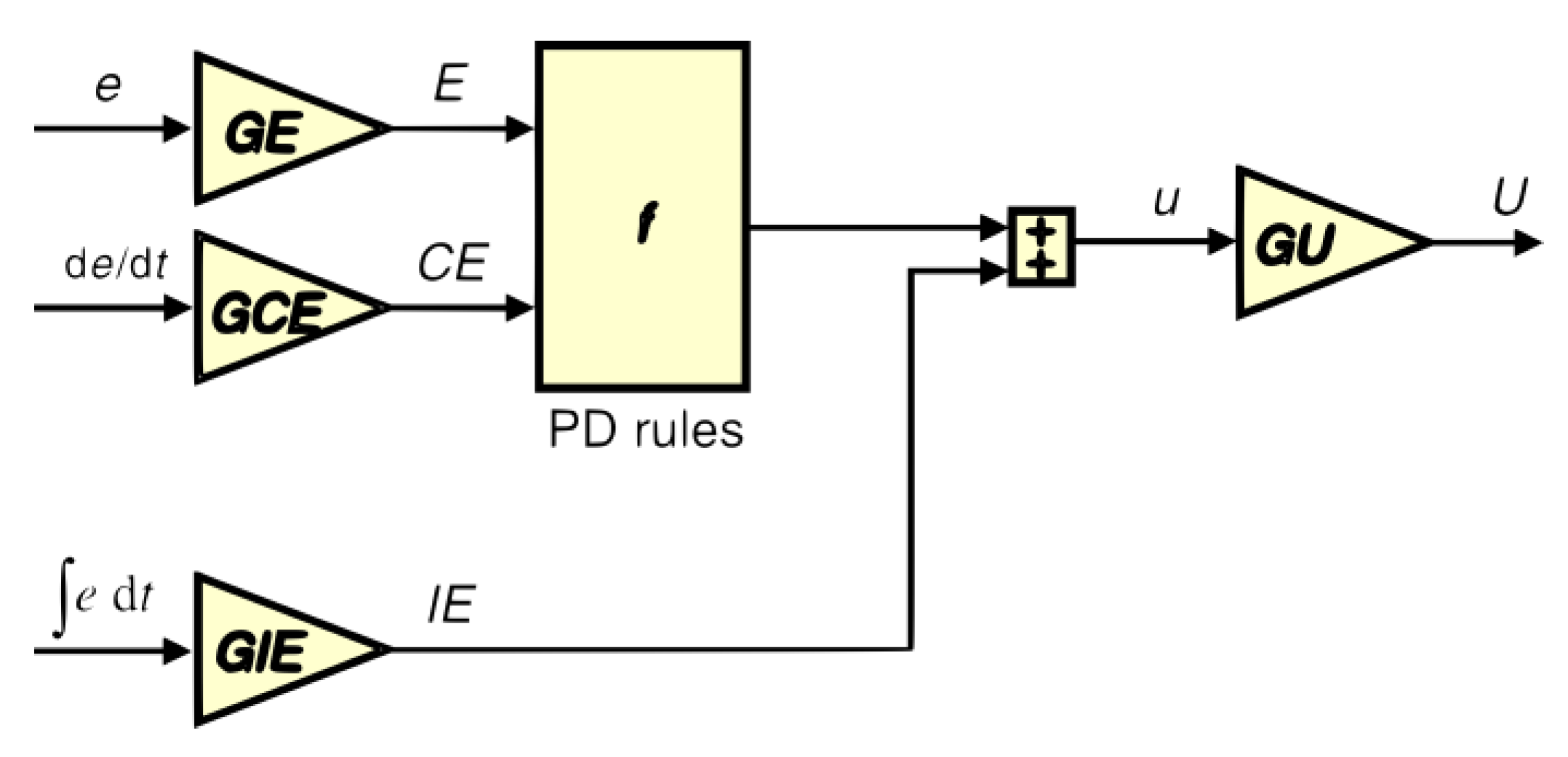
3.5.3. Linear PD-I Fuzzy Controller
| Code 16. Configuration of PD-I fuzzy controller with the UPAFuzzySystems library. | |
| 1 2 3 4 | LinearPidFuzzController = UPAfs.fuzzy_controller(Linear,typec='PD-I',tf=TF,DT = T[1], GE=15.91545709, GU=0.094248, GCE=0.636618283, GIE=7.234298678) LinearPidFuzzController.build() LinearPidFuzzControllerBlock = LinearPidFuzzController.get_controller() LinearPidFuzzSystemBlock = LinearPidFuzzController.get_system() |
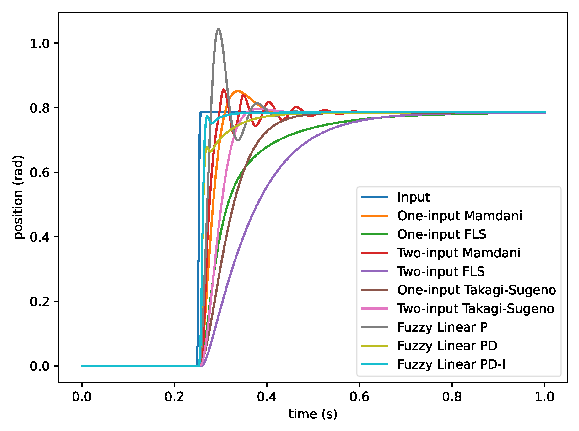
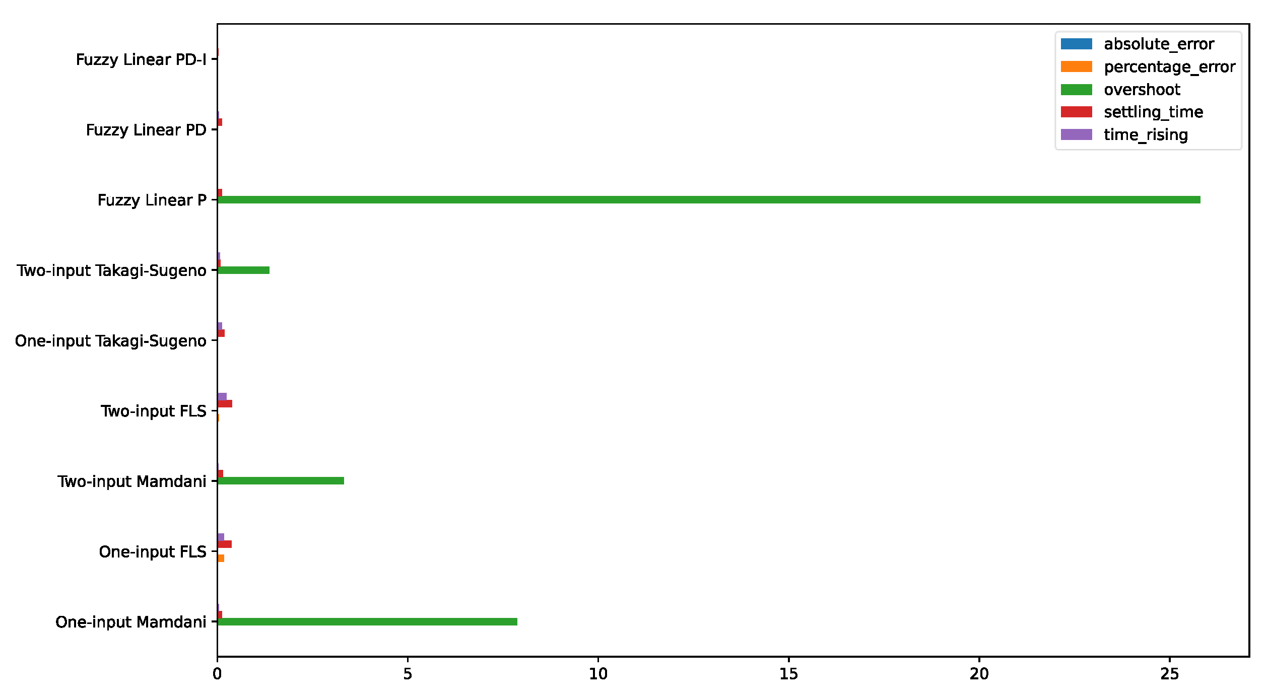
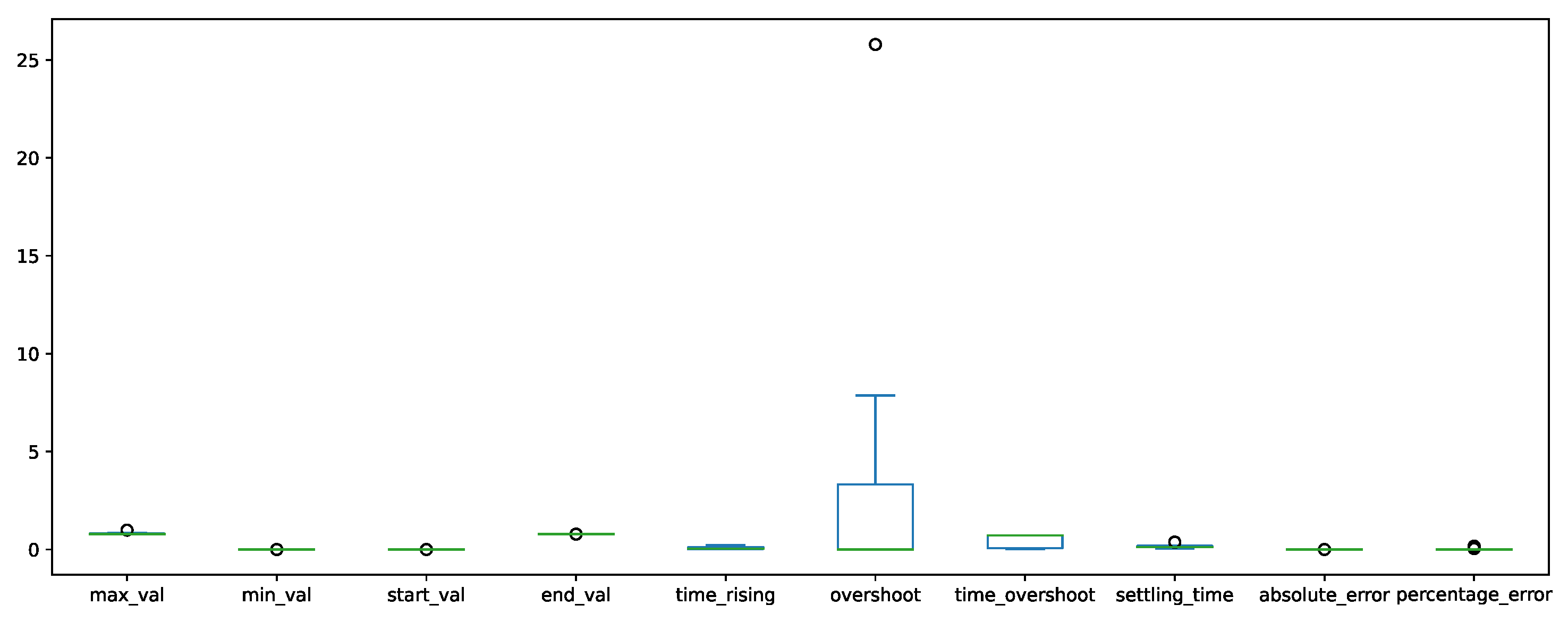
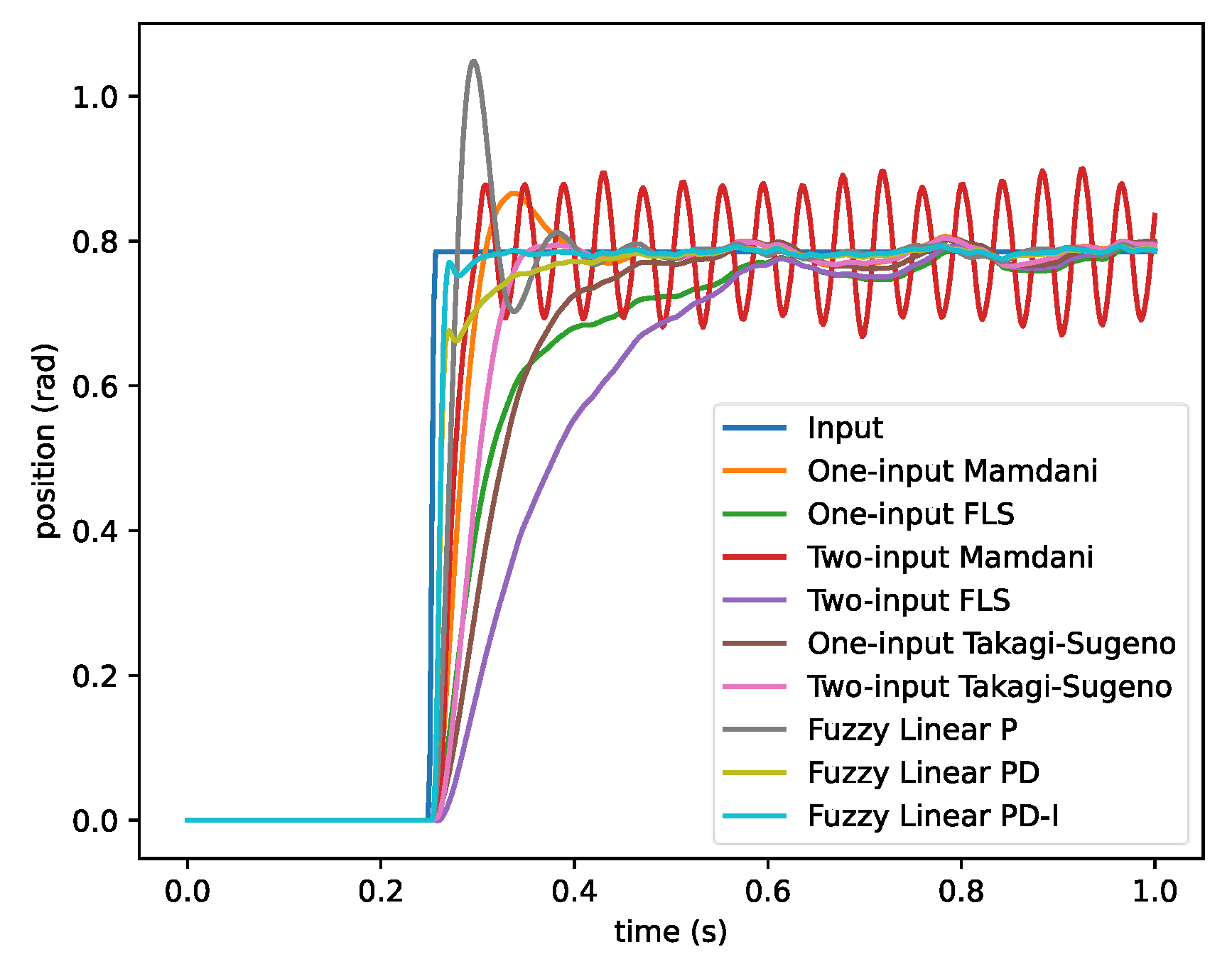
3.6. Controllers Comparison
4. Conclusions
Future Work
Author Contributions
Funding
Data Availability Statement
Conflicts of Interest
References
- Astrom, K.J.; Wittenmark, B. Adaptive Control—Astrom, 2nd ed.; Courier Corporation: North Chelmsford, MA, USA, 2008; pp. 17–38. [Google Scholar]
- Spirin, N.A.; Rybolovlev, V.Y.; Lavrov, V.V.; Gurin, I.A.; Schnayder, D.A.; Krasnobaev, A.V. Scientific Problems in Creating Intelligent Control Systems for Technological Processes in Pyrometallurgy Based on Industry 4.0 Concept. Metallurgist 2020, 64, 574–580. [Google Scholar] [CrossRef]
- Åström, K.J.; Wittenmark, B. Computer-Controlled Systems: Theory and Design; Courier Corporation: North Chelmsford, MA, USA, 2011; p. 557. [Google Scholar]
- Tarbosh, Q.A.; Aydogdu, O.; Farah, N.; Talib, M.H.N.; Salh, A.; Cankaya, N.; Omar, F.A.; Durdu, A. Review and Investigation of Simplified Rules Fuzzy Logic Speed Controller of High Performance Induction Motor Drives. IEEE Access 2020, 8, 49377–49394. [Google Scholar] [CrossRef]
- Jang, J.S.R.; Sun, C.T.; Mizutani, E. Neuro-Fuzzy and Soft Computing-A Computational Approach to Learning and Machine Intelligence [Book Review]. IEEE Trans. Autom. Control. 1997, 42, 482–1484. [Google Scholar] [CrossRef]
- Ferdaus, M.M.; Pratama, M.; Anavatti, S.G.; Garratt, M.A.; Lughofer, E. PAC: A Novel Self-Adaptive Neuro-Fuzzy Controller for Micro Aerial Vehicles. Inf. Sci. 2020, 512, 481–505. [Google Scholar] [CrossRef]
- Chen, Y.; Zhao, T.; Peng, J.; Mao, Y. Fuzzy Fraction-Order Stochastic Parallel Gradient Descent Approach for Efficient Fiber Coupling. Opt. Eng. 2022, 61, 016108. [Google Scholar] [CrossRef]
- Khanesar, M.A.; Branson, D. Robust Sliding Mode Fuzzy Control of Industrial Robots Using an Extended Kalman Filter Inverse Kinematic Solver. Energies 2022, 15, 1876. [Google Scholar] [CrossRef]
- Pereira, L.F.d.S.C.; Batista, E.; de Brito, M.A.G.; Godoy, R.B. A Robustness Analysis of a Fuzzy Fractional Order PID Controller Based on Genetic Algorithm for a DC-DC Boost Converter. Electronics 2022, 11, 1894. [Google Scholar] [CrossRef]
- Pozna, C.; Precup, R.E.; Horvath, E.; Petriu, E.M. Hybrid Particle Filter-Particle Swarm Optimization Algorithm and Application to Fuzzy Controlled Servo Systems. IEEE Trans. Fuzzy Syst. 2022, 30, 4286–4297. [Google Scholar] [CrossRef]
- Volosencu, C. MATLAB Applications in Engineering. Available online: https://www.researchgate.net/publication/358537759_MATLAB_Applications_in_Engineering (accessed on 16 February 2023).
- Zahmatkesh, S.; Klemeš, J.J.; Bokhari, A.; Rezakhani, Y.; Wang, C.; Sillanpaa, M.; Amesho, K.T.T.; Ahmed, W.S. Reducing Chemical Oxygen Demand from Low Strength Wastewater: A Novel Application of Fuzzy Logic Based Simulation in MATLAB. Comput. Chem. Eng. 2022, 166, 107944. [Google Scholar] [CrossRef]
- Maghfiroh, H.; Ahmad, M.; Ramelan, A.; Adriyanto, F. Fuzzy-PID in BLDC Motor Speed Control Using MATLAB/Simulink. J. Robot. Control 2022, 3, 8–13. [Google Scholar] [CrossRef]
- Mostafa, S.; Zekry, A.; Youssef, A.; Anis, W.R. Raspberry Pi Design and Hardware Implementation of Fuzzy-PI Controller for Three-Phase Grid-Connected Inverter. Energies 2022, 15, 843. [Google Scholar] [CrossRef]
- Lin, X.; Liu, X. Modeling and Control of One-Stage Inverted Pendulum Body Based on Matlab. J. Phys. Conf. Ser. 2022, 2224, 012107. [Google Scholar] [CrossRef]
- Kandemir, E.; Cetin, N.S.; Borekci, S. Single-Stage Photovoltaic System Design Based on Energy Recovery and Fuzzy Logic Control for Partial Shading Condition. Int. J. Circuit Theory Appl. 2022, 50, 1770–1792. [Google Scholar] [CrossRef]
- Taskin, A.; Kumbasar, T. An Open Source Matlab/Simulink Toolbox for Interval Type-2 Fuzzy Logic Systems. In Proceedings of the 2015 IEEE Symposium Series on Computational Intelligence (SSCI), Cape Town, South Africa, 7–10 December 2015; pp. 1561–1568. [Google Scholar] [CrossRef]
- Wang, J.; Niu, X.; Zheng, L.; Zheng, C.; Wang, Y. Wireless Mid-Infrared Spectroscopy Sensor Network for Automatic Carbon Dioxide Fertilization in a Greenhouse Environment. Sensors 2016, 16, 1941. [Google Scholar] [CrossRef] [PubMed]
- Wang, C.C. Fuzzy Theory-Based Air Valve Control for Auto-Score-Recognition Soprano Recorder Machines. J. Robot. Netw. Artif. Life 2021, 8, 278–283. [Google Scholar] [CrossRef]
- Singh, S.; Kaur, M. Gain Scheduling of PID Controller Based on Fuzzy Systems. MATEC Web Conf. 2016, 57, 01008. [Google Scholar] [CrossRef]
- Mehmet Karadeniz, A.; Ammar, A.; Geza, H. Comparison between Proportional, Integral, Derivative Controller and Fuzzy Logic Approaches on Controlling Quarter Car Suspension System. MATEC Web Conf. 2018, 184, 02018. [Google Scholar] [CrossRef]
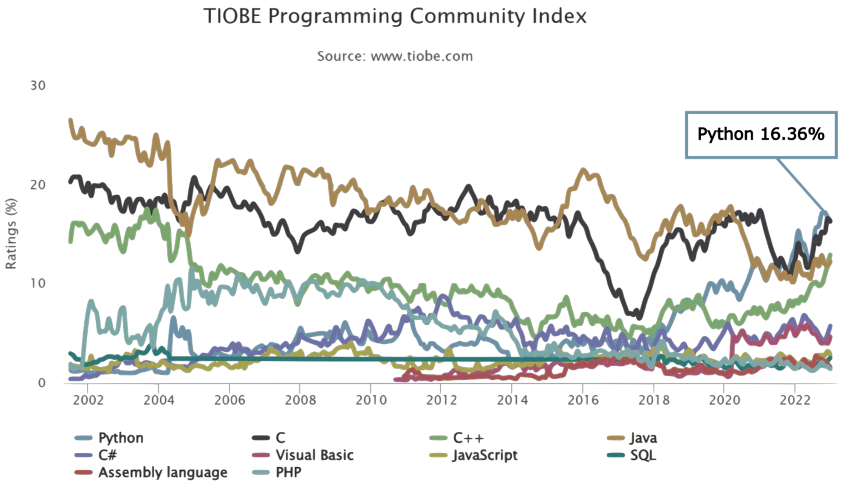
- TIOBE Index—TIOBE. Available online: https://www.tiobe.com/tiobe-index/ (accessed on 16 February 2023).
- Xu, B.; An, L.; Thung, F.; Khomh, F.; Lo, D. Why Reinventing the Wheels? An Empirical Study on Library Reuse and Re-Implementation. Empir. Softw. Eng. 2020, 25, 755–789. [Google Scholar] [CrossRef]
- Rueden, C.T.; Schindelin, J.; Hiner, M.C.; DeZonia, B.E.; Walter, A.E.; Arena, E.T.; Eliceiri, K.W. ImageJ2: ImageJ for the next Generation of Scientific Image Data. BMC Bioinform. 2017, 18, 529. [Google Scholar] [CrossRef] [PubMed]
- Macmillan, M.; Eurek, K.; Cole, W.; Bazilian, M.D. Solving a Large Energy System Optimization Model Using an Open-Source Solver. Energy Strategy Rev. 2021, 38, 100755. [Google Scholar] [CrossRef]
- Guo, Y.; Leitner, P. Studying the Impact of CI on Pull Request Delivery Time in Open Source Projects—A Conceptual Replication. PeerJ Comput. Sci. 2019, 5, e245. [Google Scholar] [CrossRef] [PubMed]
- Shields.Io: Quality Metadata Badges for Open Source Projects. Available online: https://shields.io/ (accessed on 24 January 2023).
- GitHub—Luferov/FuzzyLogicToolBox: Fuzzy Logic Library for Python. Available online: https://github.com/Luferov/FuzzyLogicToolBox (accessed on 23 January 2023).
- Avelar, E.; Castillo, O.; Soria, J. Fuzzy Logic Controller with Fuzzylab Python Library and the Robot Operating System for Autonomous Robot Navigation: A Practical Approach. Stud. Comput. Intell. 2020, 862, 355–369. [Google Scholar] [CrossRef]
- ITTcs/Fuzzylab: Fuzzylab, a Python Fuzzy Logic Library. Available online: https://github.com/ITTcs/fuzzylab (accessed on 23 January 2023).
- GitHub—Yudivian/Fuzzython: Fuzzy Logic and Fuzzy Inference Python 3 Library. Available online: https://github.com/yudivian/fuzzython (accessed on 24 January 2023).
- GitHub—Carmelgafa/Type2fuzzy: Type-2 Fuzzy Logic Library. Available online: https://github.com/carmelgafa/type2fuzzy (accessed on 24 January 2023).
- Fuzzylite/Pyfuzzylite: Pyfuzzylite: A Fuzzy Logic Control Library in Python. Available online: https://github.com/fuzzylite/pyfuzzylite (accessed on 24 January 2023).
- Montes Rivera, M. GitHub—UniversidadPolitecnicaAguascalientes/UPAFuzzySystems. Available online: https://github.com/UniversidadPolitecnicaAguascalientes/UPAFuzzySystems (accessed on 1 March 2023).
- Nguyen, H.T. A First Course in Fuzzy and Neural Control; Chapman & Hall/CRC Press: London, UK, 2003; ISBN 9781584882442. [Google Scholar]
- Jantzen, J. Foundations of Fuzzy Control: A Practical Approach, 2nd ed.; John Wiley & Sons: Hoboken, NJ, USA, 2013; pp. 1–325. [Google Scholar] [CrossRef]
- Dehghani, M.; Taghipour, M.; Gharehpetian, G.B.; Abedi, M. Optimized Fuzzy Controller for MPPT of Grid-Connected PV Systems in Rapidly Changing Atmospheric Conditions. J. Mod. Power Syst. Clean Energy 2021, 9, 376–383. [Google Scholar] [CrossRef]
- Sao, K.; Kumar Singh, D.; Agrawal, A.; Scholar, P.; Professor, A.; Raman, D. Study of DC Motor Position Control Using Root Locus and PID Controller in MATLAB. IJSRD-Int. J. Sci. Res. Dev. 2015, 3, 183–190. [Google Scholar]


| Library | Design of FISs | Design of FISs Controllers | PID FISs Controllers | Simulation of FISs Controllers with Transfer Functions and State-Space Models |
|---|---|---|---|---|
| Fuzzy-logic-toolbox | Yes | No | No | No |
| Scikit-fuzzy | Yes | Yes (Only Mamdani controller) | No | No |
| fuzzylab | Yes | No | No | No |
| fuzzython | Yes | No | No | No |
| Type2Fuzzy | Yes (Type 2) | No | No | No |
| Fuzzy-machines | Yes | No | No | No |
| pyfuzzylite | Yes | Yes | No | No |
| Simpful | Yes | No | No | No |
| pyFume | Yes | No | No | No |
| UPAFuzzySystems | Yes | Yes | Yes | Yes |
| FIS Controller | Input Universes | Connectives | IF-THEN Rules | Defuzzification |
|---|---|---|---|---|
| Mamdani | Not defined | Equations (7) and (8) | Equation (11) | Equations (14) and (16) |
| FLS | [−1, 1] | Equations (9) and (10) | Equation (11) | Equation (17) |
| Linear | [−100, 100] | Equations (9) and (10) | Equation (13) | Equation (15) |
| Takagi–Sugeno | Not defined | Equations (9) and (10) | Equation (13) | Equation (15) |
| Linear P | [−100, 100] | Equations (9) and (10) | Equation (13) | Equation (15) |
| Linear PD | [−100, 100] | Equations (9) and (10) | Equation (13) | Equation (15) |
| Linear PID | [−100, 100] | Equations (9) and (10) | Equation (13) | Equation (15) |
| No-linear P | Not defined | Equations (7) and (8) | Equation (11) | Equations (14) and (16) |
| No-linear PD | Not defined | Equations (7) and (8) | Equation (11) | Equations (14) and (16) |
| No-linear PID | Not defined | Equations (7) and (8) | Equation (11) | Equations (14) and (16) |
| FIS Controller | Example of Rules |
|---|---|
| Mamdani | One input: If error is Neg then control is Neg If error is Zero then control is Zero If error is Pos then control is Pos Two input: If error is Neg and change error is Neg then control is Neg If error is Neg and change error is Zero then control is Neg If error is Zero and change error is Neg then control is Zero If error is Neg and change error is Pos then control is Zero If error is Zero and change error is Zero then control is Zero If error is Zero and change error is Pos then control is Zero If error is Pos and change error is Neg then control is Zero if error is Pos and change error is Zero then control is Pos If error is Pos and change error is Pos then control is Pos |
| FLS | One input: If error is Neg then control is Neg If error is Zero then control is Zero If error is Pos then control is Pos Two input: If error is Neg and change error is Neg then control is Neg If error is Neg and change error is Zero then control is Neg If error is Zero and change error is Neg then control is Zero If error is Neg and change error is Pos then control is Zero If error is Zero and change error is Zero then control is Zero If error is Zero and change error is Pos then control is Zero If error is Pos and change error is Neg then control is Zero if error is Pos and change error is Zero then control is Pos If error is Pos and change error is Pos then control is Pos |
| Linear | One input: If error is Neg then control is −100 If error is Zero then control is 0 If error is Pos then control is 100 Two inputs: If error is Neg and change error is Neg then control is −200 If error is Neg and change error is Pos then control is 0 If error is Pos and change error is Neg then control is 0 If error is Pos and change error is Pos then control is 200 |
| Takagi–Sugeno | One input: If error is Neg then control is If error is Zero then control is 0 If error is Pos then control is c Two inputs: If error is Neg and change error is Neg then control is If error is Neg and change error is Pos then control is 0 If error is Pos and change error is Neg then control is 0 If error is Pos and change error is Pos then control is |
| Linear P | If error is Neg then control is −100 If error is Zero then control is 0 If error is Pos then control is 100 |
| Linear PD | If error is Neg and change error is Neg then control is −200 If error is Neg and change error is Pos then control is 0 If error is Pos and change error is Neg then control is 0 If error is Pos and change error is Pos then control is 200 |
| Linear PID | If error is Neg and change error is Neg then control is −200 If error is Neg and change error is Pos then control is 0 If error is Pos and change error is Neg then control is 0 If error is Pos and change error is Pos then control is 200 |
| Parameter | Description | Value |
|---|---|---|
| Inertial Coefficient | ||
| Viscous Friction Coefficient | ||
| Electromotive Force | 0.0274 | |
| Armor Resistance | 4 Ω | |
| Armor Inductance | H | |
| Simulation Time | 1.0 s | |
| Total Number of Samples | 1500 | |
| Transfer Function |
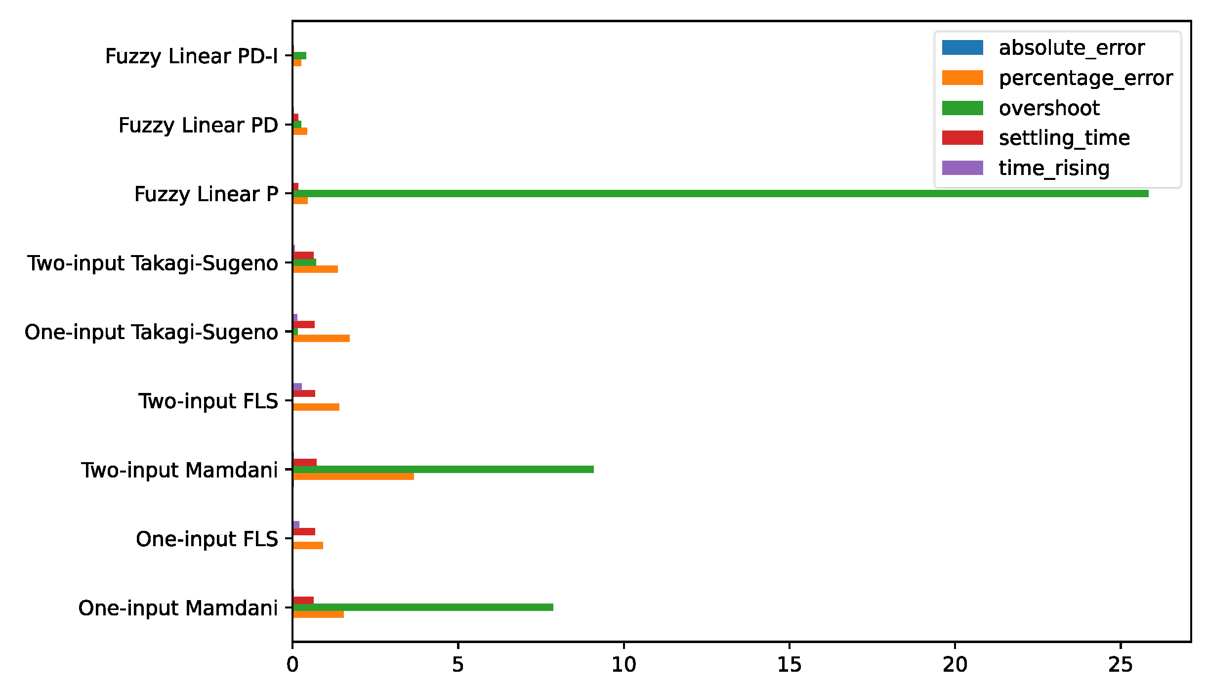
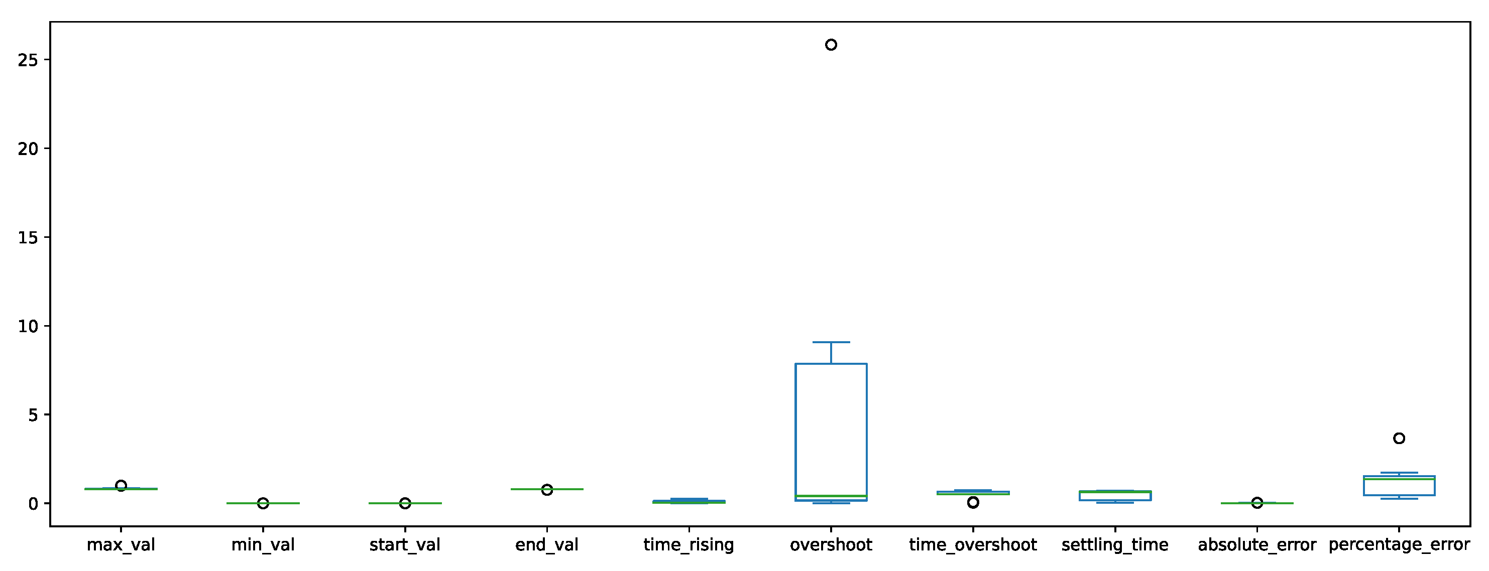
| Fuzzy Controller | One-Input Mamdani | One-Input FLS | Two-Input Mamdani | Two-Input FLS | One-Input Takagi–Sugeno | Two-input Takagi–Sugeno | Fuzzy Linear P | Fuzzy Linear PD | Fuzzy Linear PD-I |
|---|---|---|---|---|---|---|---|---|---|
| max_val (rad) | |||||||||
| min_val (rad) | 0.00 | 0.00 | 0.00 | 0.00 | 0.00 | 0.00 | |||
| start_val (rad) | 0.00 | 0.00 | 0.00 | 0.00 | 0.00 | 0.00 | 0.00 | ||
| end_val (rad) | |||||||||
| time_rising (s) | |||||||||
| Overshoot (s) | 0.00 | 9.09 | 0.00 | ||||||
| time_overshoot (s) | |||||||||
| settling_time (s) | |||||||||
| Absolute Error (rad) | |||||||||
| Percentage Error (%) | 3.66 | 1.41 | 1.37 |
| sum_sq | df | F | PR(>F) | |
|---|---|---|---|---|
| C(features) | 0.164450 | 3.0 | 9.066149 | 0.000172 |
| Residual | 0.193481 | 32.0 |
| Fuzzy Controller | One-Input Mamdani | One-Input FLS | Two-Input Mamdani | Two-Input FLS | One-Input Takagi–Sugeno | Two-Input Takagi–Sugeno | Fuzzy Linear P | Fuzzy Linear PD | Fuzzy Linear PD-I |
|---|---|---|---|---|---|---|---|---|---|
| max_val (rad) | |||||||||
| min_val (rad) | |||||||||
| start_val (rad) | |||||||||
| end_val (rad) | |||||||||
| time_rising (s) | |||||||||
| Overshoot (s) | |||||||||
| time_overshoot (s) | |||||||||
| settling_time (s) | |||||||||
| Absolute Error (rad) | |||||||||
| Percentage Error (%) |
| Sum_sq | df | F | PR(>F) | |
|---|---|---|---|---|
| C(features) | 9.535859 | 3.0 | 11.074266 | 0.000038 |
| Residual | 9.184882 | 32.0 |
Disclaimer/Publisher’s Note: The statements, opinions and data contained in all publications are solely those of the individual author(s) and contributor(s) and not of MDPI and/or the editor(s). MDPI and/or the editor(s) disclaim responsibility for any injury to people or property resulting from any ideas, methods, instructions or products referred to in the content. |
© 2023 by the authors. Licensee MDPI, Basel, Switzerland. This article is an open access article distributed under the terms and conditions of the Creative Commons Attribution (CC BY) license (https://creativecommons.org/licenses/by/4.0/).
Share and Cite
Montes Rivera, M.; Olvera-Gonzalez, E.; Escalante-Garcia, N. UPAFuzzySystems: A Python Library for Control and Simulation with Fuzzy Inference Systems. Machines 2023, 11, 572. https://doi.org/10.3390/machines11050572
Montes Rivera M, Olvera-Gonzalez E, Escalante-Garcia N. UPAFuzzySystems: A Python Library for Control and Simulation with Fuzzy Inference Systems. Machines. 2023; 11(5):572. https://doi.org/10.3390/machines11050572
Chicago/Turabian StyleMontes Rivera, Martín, Ernesto Olvera-Gonzalez, and Nivia Escalante-Garcia. 2023. "UPAFuzzySystems: A Python Library for Control and Simulation with Fuzzy Inference Systems" Machines 11, no. 5: 572. https://doi.org/10.3390/machines11050572