Vibration Modeling and Analysis of a Flexible 3-PRR Planar Parallel Manipulator Based on Transfer Matrix Method for Multibody System

Abstract

This paper presents the vibration model of a 3-prismatic–revolute–revolute (PRR) planar parallel manipulator (PPM) with three flexible intermedia links, utilizing the linear transfer matrix method for multibody systems (MSTMM). The dynamic characteristics of the PRR PPM are also investigated. The dynamic model of the 3-PRR PPM is derived, and the transfer matrix and transfer equation of each component in the system, as well as the overall transfer equation and transfer matrix of the system are obtained. The vibration characteristics of the whole system are determined using the MSTMM and verified through ANSYS simulation. Furthermore, the relationship between the natural frequencies and the flexible PPM configurations is analyzed under a specific circular trajectory. The results demonstrate that the natural frequency of the system changes constantly with the configurations, and the trends of the first six orders are similar. This novel modeling approach does not require global dynamic equations and is both efficient and accurate. Moreover, it can be easily extended to other parallel manipulators with flexible components.

1. Introduction

Compared with series manipulators, parallel manipulators have the advantages of high precision, high speed, and strong load capacity [1]. Therefore, they are widely used in precision manufacturing [2], automatic microassembly [3], surgical robots [4], and other applications. As the speed and acceleration of the rigid manipulator are limited, some scholars have proposed and designed lightweight manipulators that use flexible components instead of the original rigid components. However, the flexible elements in the parallel manipulators are prone to vibration and deformation, which can seriously affect the system’s operational accuracy, stability, and dynamic performance [5]. Therefore, during the process of dynamic modeling of the manipulators, the elastic vibration of flexible components cannot be ignored. Simultaneously, the analysis of vibration characteristics is an essential research topic in dynamics. Frequency analysis can help to understand the vibration characteristics of parallel manipulators, providing vital theoretical guidance for robot design and vibration suppression [6,7].

The process of dynamic modeling and analysis for flexible parallel manipulators is significantly more complex compared with rigid parallel manipulators. Firstly, it is necessary to discretize the flexible bar, and then use a dynamic method for modeling. Currently, common methods for studying the dynamics of flexible parallel manipulators include the finite element method, modal analysis, and others. For instance, Zhang et al. established the dynamic model of the 3-PRR parallel manipulator with three flexible intermediate links based on the hypothetical mode method and verified the vibration control [8]. Gao et al. established an N-dimensional discrete dynamic model of a two-link flexible manipulator based on the hypothetical mode method and achieved trajectory tracking and vibration suppression [9]. Pira studied the dynamics of a 3-PRR planar parallel manipulator with flexible links by the finite element method and analyzed the natural frequency characteristics of the system [10]. Li analyzed the natural frequency, mode, dynamic response, and frequency characteristics of the compliant mechanism using the finite element method [11]. Wang and Mills used the Lagrangian finite element method to establish the dynamic model of flexible planar linkage with two translational degrees of freedom and one rotational degree of freedom, studying the vibration suppression of flexible linkage [12]. Furthermore, in the work by Mahboubkhah et al., researchers developed a dynamic model for the flexible Stewart platform using the finite element method and studied the comprehensive free vibration of the machine tool hexapod worktable [13].

These methods have been widely used for modeling the dynamics of flexible parallel manipulators, especially the finite element method, which is the mainstream method for describing flexible body deformation in the dynamics of most flexible multibody systems because of its strong generality [14,15,16]. However, when these methods are used to calculate the vibration characteristics of rigid-flexible multibody systems, the global dynamics equations of the system must be established. Often, they need to be rederived as the system topology changes [17,18]. On the other hand, the order of the system matrix depends on the degrees of freedom of the system. For complex multi-body systems with multiple degrees of freedom, the higher order of the system matrix, along with complex discretization operations and a large number of numerical calculations, can result in large computational effort and computational pathologies caused by large stiffness gradients [19].

To simplify the research process, eliminate the need for establishing the global dynamics equations of the system, and achieve accurate dynamics modeling and fast computation of the system, Rui developed a new multibody system modeling method called the transfer matrix method for multibody systems (MSTMM) [20,21]. This method decomposes a complex multibody system into various components, such as rigid bodies, flexible bodies, hinges, and concentrated masses. Then, the transfer matrix is established for each of these components. By assembling the transfer matrices of each element according to their connection relations, the overall transfer equation and transfer matrix of the whole system can be derived. Subsequently, the vibration characteristics of the system can be obtained by solving its characteristic equation. The linear MSTMM does not require the establishment of the global dynamics equations of the system. Instead, it replaces the overall system characteristic equations with the overall system transfer equations, avoiding the complex rigid-flexible multibody system vibration characteristics calculation pathology, and ensuring the rapid solution of the system eigenvalues. This greatly improves the computational efficiency [22,23].

The linear transfer matrix method for multibody systems (MSTMM) has been developed in recent years as a method to study multibody system dynamics by using transfer matrices [24]. Compared with other dynamic modeling methods, the linear MSTMM has the characteristics of accurate and efficient calculation without global dynamic modeling. Therefore, it is widely used in the fields of vehicles, aerospace [25], and marine engineering [26,27]. In this paper, the vibration model of the flexible 3-PRR PPM is established using linear MSTMM, and the numerical simulation is carried out using ANSYS software. The main contributions of this paper are as follows. (1) The extension of the research work on linear MSTMM to include vibration modeling of the 3-PRR planar parallel manipulator, and the use of this method to solve for the natural frequencies of the system. (2) Analysis of the relationship between natural frequencies and configurations of the flexible 3-PRR PPM using linear MSTMM. Furthermore, the method proposed in this paper can be easily applied to the vibration modeling of other parallel manipulators with flexible components, thus laying a foundation for dynamic optimization.

2. Introduction of the Linear MSTMM

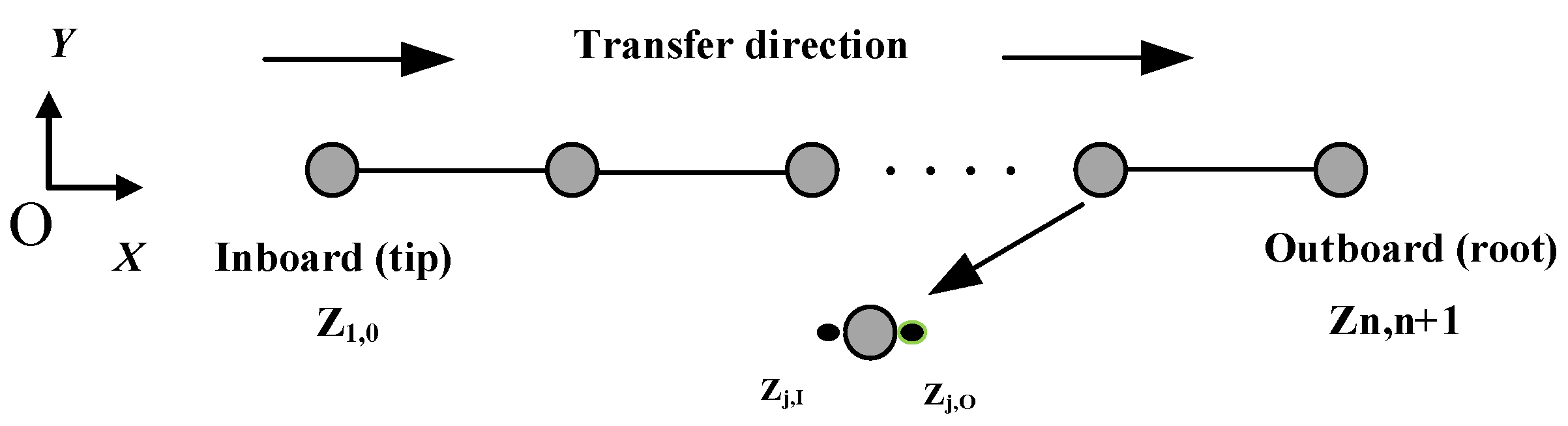
State Vector, Transfer Matrix, and Transfer Equation

The basic concepts of the transfer matrix method include the state vector and transfer equation, which together form the dynamic system. Each body element in a multibody system contains at least one input state vector and one output state vector, which represent displacements (including orientation angle displacements) and internal forces (including interior torques) of the element [28].

For a planar vibration system, the state vectors of the connection points are defined as:

$$z_I={{\left[\begin{array}{cccccc}x& y& {\theta }_z& m_z& q_x& q_y\end{array}\right]}^{\mathrm{T}}}_I$$

(1)

$$z_O={{\left[\begin{array}{cccccc}x& y& {\theta }_z& m_z& q_x& q_y\end{array}\right]}^{\mathrm{T}}}_O$$

(2)

where $x$ and $y$ represent the physical translation of the element, ${\theta }_z$ is the orientation angle, $m_z$, $q_x$ and $q_y$ are the internal torque and internal force, respectively.

The solution of the free vibration of the system can be obtained by superposition of the principal modes. The modal transformation can be expressed as:

$$z={Ze}^{i\omega t}$$

(3)

The state vectors of the system in the modal coordinate are defined as:

$$Z_I={{\left[\begin{array}{cccccc}X& Y& {\Theta }_z& {{\rm M}}_z& Q_x& Q_y\end{array}\right]}^{\mathrm{T}}}_I$$

(4)

$$Z_O={{\left[\begin{array}{cccccc}X& Y& {\Theta }_z& {{\rm M}}_z& Q_x& Q_y\end{array}\right]}^{\mathrm{T}}}_O$$

(5)

$Z_I$ and $Z_O$ are the modal coordinates corresponding to physical coordinates, which represent the amplitude of displacement, angle, internal torque, and internal force. $\omega$ represents the natural frequency of the system.

Taking the chain system shown in Figure 1 as an example, the transfer equation of element $j$ can be obtained easily from the dynamic equation and expressed as:

$$Z_{j,j+1}=U_j{Z}_{j,j-1}$$

(6)

where $U_j$ is the transfer matrix of component j.

For a multibody system composed of $n$ elements, the overall transfer matrix of the system can be obtained by [29]:

$${\mathit{Z}}_{\mathit{n},\mathit{n}\mathbf{+}\mathbf{1}}=U_{\mathit{a}\mathit{l}\mathit{l}}{\mathit{Z}}_{\mathrm{1,0}}$$

(7)

$$U_{all}=U_1{U}_2{U}_3\dots U_n$$

(8)

$U_{all}$ is the overall transfer matrix of the system. Equations (7) and (8) show that in MSTMM, there is no need to establish global dynamics equations for the system. The dimensionality of the transfer matrix depends only on the number of the boundary state vectors at the input and output of the system, and it does not increase with an increase in degrees of freedom. This approach keeps the overall transfer equations low-order, resulting in improved computational efficiency and accuracy, even for complex multibody systems.

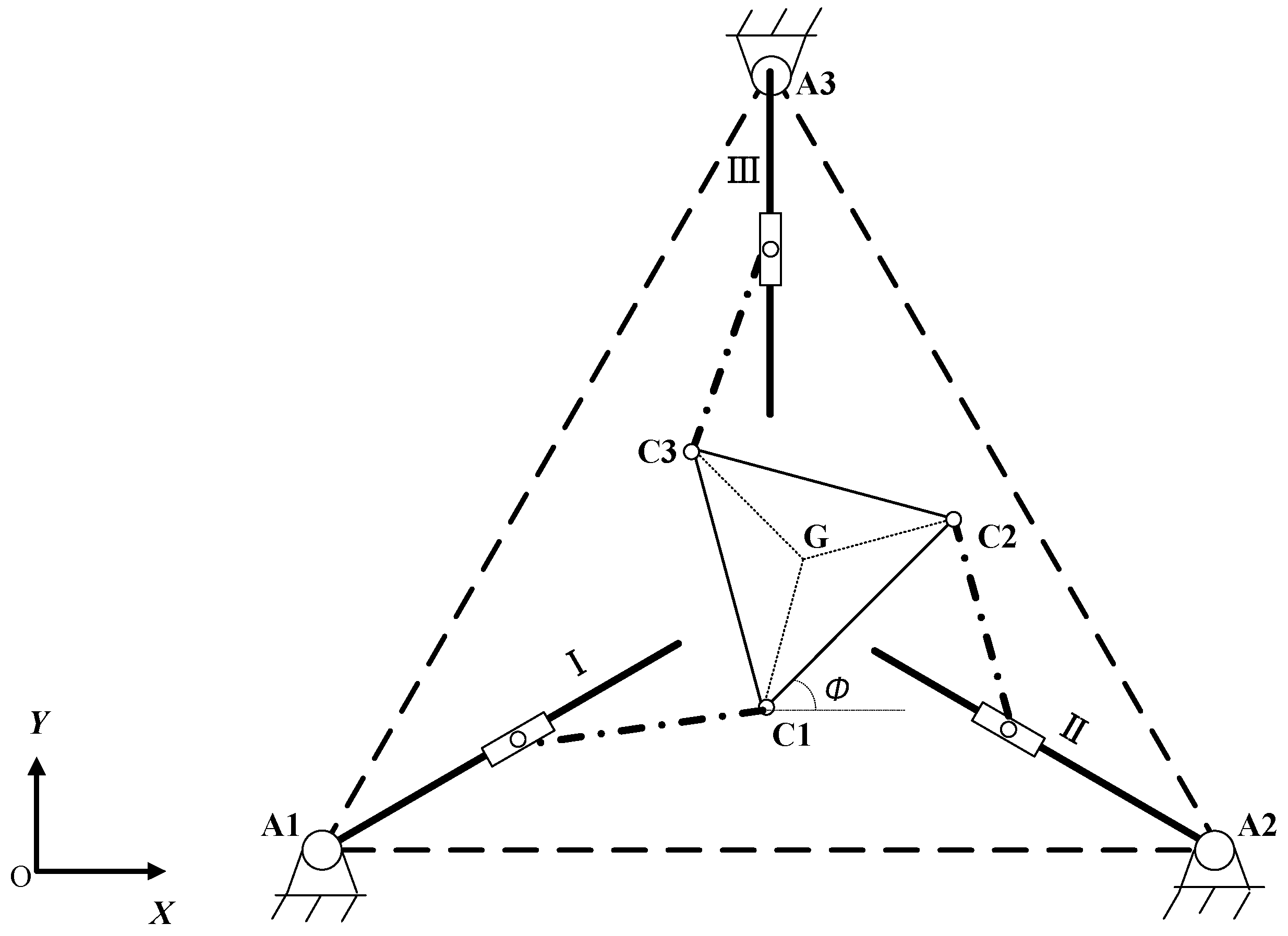
3. Dynamic Model of the Flexible 3-PRR PPM

The structure of the flexible 3-PRR PPM is shown in Figure 2. It consists of a regular triangle mobile platform $C_1{C}_2{C}_3$, with three closed branch chains connected to the fixed base platform $A_1{A}_2{A}_3$. Each branch chain has an active moving joint and two passive rotating joints that move along the straight line of the guideway [30,31]. The global coordinate system $OXY$ is set at the position of the base platform $A_1$, and the initial angle of the mobile platform is expressed as ${\phi .}_{}$

The PPM can be modeled as a linear flexible multibody system that includes flexible links, sliders, mobile platforms, and smooth hinges. To model these components, it is necessary to derive their transfer matrices.

3.1. Transfer Matrix of the Mobile Platform

The mobile platform can be considered as a rigid body with three inputs and one output [32]. The structure diagram shown in Figure 3 illustrates the three input points, denoted as $I_1,I_2,I_3$, and the output located at the center $G$ of the mobile platform. The first moving coordinate system $O_1{X}_1{Y}_1$ is fixed at point $I_1$ and is parallel to the global coordinate system. In this case, the initial angle between the mobile platform and the first moving coordinate system is ${\phi }_{}$. The $x$-axis of the moving coordinate system $O_1{X}_2{Y}_2$ of the platform is oriented along the direction from point $I_1$ to the point $I_2$.

In the plane coordinate system $O_1{X}_2{Y}_2$, the angular relationship of a rigid body undergoing small vibrations can be obtained as:

$${\theta }_{I_j}={\theta }_{I_1} (j=\mathrm{2,3})$$

(9)

$${\theta }_{OG}={\theta }_{I_1}$$

(10)

For a multi-input-single-output rigid body with linear vibration, the displacements of the remaining input points and output points can be expressed as a function of the displacement of the first input point $I_1$ and the angular displacement around $I_1$:

$$\left[\begin{array}{c}{x}_{I_j{,I}_1}^{}\\ y_{I_j,I_1}^{}\end{array}\right]=\left[\begin{array}{c}{x}_{I_1}^{}\\ y_{I_1}^{}\end{array}\right]+\left[\begin{array}{c}{-y}_{I_j}\\ x_{I_j}\end{array}\right]{\theta }_{I_1} (j=\mathrm{2,3})$$

(11)

$$\left[\begin{array}{c}{x}_{OG{,I}_1}^{}\\ y_{OG,I_1}^{}\end{array}\right]=\left[\begin{array}{c}{x}_{I_1}^{}\\ y_{I_1}\end{array}\right]+\left[\begin{array}{c}{-y}_{OG}^{}\\ x_{OG}^{}\end{array}\right]{\theta }_{I_1}$$

(12)

where $(x_{I_j}^{},y_{I_j}^{})$,$(x_{OG}^{},y_{OG}^{})$ are the position coordinates of the input point $I_j$ and the output point $G$ in the moving coordinate system, respectively.

By combining Equations (9) and (11) and rewriting the relationship between position and angle into matrix form using Equations (1)–(3), we get:

$$U_{I_j}{Z}_{I_1}+U_{I_1}{Z}_{I_j}=0_{3\times 1} (j=\mathrm{2,3})$$

(13)

where $Z_{I_1}$, $Z_{I_2},$ and $Z_{I_3}$ denote the state vectors of three inputs, and

$$U_{I_j}=\left[\begin{array}{cc}\begin{array}{ccc}1& 0& {-y}_{I_j}\\ 0& 1& x_{I_j}\\ 0& 0& 1\end{array}& \begin{array}{ccc}0& 0& 0\\ 0& 0& 0\\ 0& 0& 0\end{array}\end{array}\right](j=\mathrm{2,3})$$

(14)

$$U_{I_1}=\left[\begin{array}{cc}\begin{array}{ccc}1& 0& 0\\ 0& 1& 0\\ 0& 0& 1\end{array}& \begin{array}{ccc}0& 0& 0\\ 0& 0& 0\\ 0& 0& 0\end{array}\end{array}\right]$$

(15)

Similarly, Equations (10) and (12) are also rewritten into matrix form as:

$${\mathit{U}}_{\mathit{G}}{\mathit{Z}}_{{\mathit{I}}_1}+U_{I_1}{Z}_G=0_{3\times 1}$$

(16)

where $Z_G$ denotes the state vectors of output, and

$$U_G=\left[\begin{array}{cc}\begin{array}{ccc}1& 0& {-y}_{O_G}\\ 0& 1& x_{O_G}\\ 0& 0& 1\end{array}& \begin{array}{ccc}0& 0& 0\\ 0& 0& 0\\ 0& 0& 0\end{array}\end{array}\right]$$

(17)

For a multi-input-single-output mobile platform in free vibration, where no external force is applied, the advection equation can be obtained as:

$$q_{x,G}^O={\sum }_{j=1}^3{q}_{x,j}^I-m_G{\ddot{x}}_{OG}$$

(18)

$$q_{y,G}^O={\sum }_{j=1}^3{q}_{y,j}^I-m_G{\ddot{y}}_{OG}$$

(19)

Here, $q_{x,j}^I$ and $q_{y,j}^I$ are the internal forces acting in the $x$ and $y$ directions at the inputs, respectively, while $q_{x,G}^O$ and $q_{y,G}^O$ are the internal forces acting in the $x$ and $y$ directions at the output. Furthermore, $m_G$ represents the mass of the center of mass, and ${\ddot{x}}_{OG}$ and ${\ddot{y}}_{OG}$ denote the accelerations at the center of mass of the mobile platform.

Considering the moment balance, the rotation equation of the input $I_1$ can be expressed as:

$$\frac{d{G}_I}{dt}+m{r}_{IC}\times a_I=M$$

(20)

Linearizing Equations (18)–(20) and combining them with Equations (1)–(3), the equations can be rewritten in matrix form as:

$$U_{I_1}^4{Z}_{I_1}+U_{I_2}^4{Z}_{I_2}+U_{I_3}^4{Z}_{I_3}+U_G^4{Z}_G=0_{3\times 1}$$

(21)

Defining the state vectors of the input and output of the mobile platform in integral forms, they can be expressed as:

$$Z_{tol}={\left[Z_{I_1}^T{Z}_{I_2}^T{Z}_{I_3}^T{Z}_G^T\right]}^{\mathrm{T}}$$

(22)

Therefore, by combining Equations (13), (16), and (21), the transfer equation of the mobile platform can be obtained as:

$$U_P{Z}_{tol}={\mathbf{0}}_{12\times 1}$$

(23)

where the transfer matrix of the mobile platform is expressed as:

$$U_P=\left[\begin{array}{cccc}{U}_{I_2}& U_{I_1}& O_{3\times 6}& O_{3\times 6}\\ U_{I_3}& O_{3\times 6}& U_{I_1}& O_{3\times 6}\\ {U_G}_{}& O_{3\times 6}& O_{3\times 6}& U_{I_1}\\ U_{I_1}^4& U_{I_2}^4& U_{I_3}^4& U_G^4\end{array}\right]$$

(24)

where:

$$U_{I1}^4=\left[\begin{array}{cc}\begin{array}{ccc}-m{y}_C{\omega }^2& m{x}_C{\omega }^2& J_{I_1}{\omega }^2\\ -m{\omega }^2& 0& m{y}_C{\omega }^2\\ 0& -m{\omega }^2& -m{x}_C{\omega }^2\end{array}& \begin{array}{ccc}1& 0& 0\\ 0& 1& 0\\ 0& 0& 1\end{array}\end{array}\right]$$

(25)

$$U_{Ij}^4=\left[\begin{array}{cc}\begin{array}{ccc}0& 0& 0\\ 0& 1& 0\\ 0& 0& 1\end{array}& \begin{array}{ccc}1& y_{I_j}& {-x}_{I_j}\\ 0& 0& 0\\ 0& 0& 0\end{array}\end{array}\right](j=\mathrm{2,3})$$

(26)

$$U_G^4=\left[\begin{array}{cc}\begin{array}{ccc}1& 0& 0\\ 0& 1& 0\\ 0& 0& 1\end{array}& \begin{array}{ccc}1& y_{O_G}& x_{OG}\\ 0& 1& 0\\ 0& 0& 1\end{array}\end{array}\right]$$

(27)

In the transfer matrix, $x_C$ and $y_C$ represent the positions of the center of the mobile platform, and $J_{I_1}$ is the moment of inertia of the mobile platform relative to $I_1$.

3.2. Transfer Matrix of the Slider

The structural diagram of the slider is shown in Figure 4. Since the volume of the slider is small compared with the other rigid bodies in the system, it can be neglected and treated as a concentrated mass. From the characteristics of concentrated masses, the following equations can be obtained: $x^O=x^I$, $y^O=y^I$, ${\theta }_z^O={\theta }_z^I$, $M_z^O=M_z^I$.

From the force relationship:

$$q_y^O=q_y^I-m_s{\ddot{y}}^I$$

(28)

$$q_x^O=q_x^I-m_s{\ddot{x}}^I$$

(29)

Similarly, $q_x^I$ and $q_y^I$ represent the internal forces acting in the $x$ and $y$ directions at the input, respectively, while $q_x^O$ and $q_y^O$ are the internal forces acting in the $x$ and $y$ directions at the output. $m_s$ represents the mass at the center of mass of the slider, and ${\ddot{x}}^I$ and ${\ddot{y}}^I$ are the accelerations at the center of mass of the slider.

The form of the slider state vector can be defined as shown in Equations (4) and (5). Therefore, the slider transfer equation and transfer matrix for the concentrated mass can be obtained as:

$$Z_o=U_{slide}{Z}_I=\left[\begin{array}{ccc}\begin{array}{c}1\\ 0\\ 0\end{array}& \begin{array}{c}0\\ 1\\ 0\end{array}& \begin{array}{c}\begin{array}{ccc}0& 0& \begin{array}{cc}0& 0\end{array}\end{array}\\ \begin{array}{ccc}0& 0& \begin{array}{cc}0& 0\end{array}\end{array}\\ \begin{array}{ccc}1& 0& \begin{array}{cc}0& 0\end{array}\end{array}\end{array}\\ 0& 0& \begin{array}{ccc}0& 1& \begin{array}{cc}0& 0\end{array}\end{array}\\ \begin{array}{c}m{\omega }^2\\ 0\end{array}& \begin{array}{c}0\\ {m\omega }^2\end{array}& \begin{array}{c}\begin{array}{ccc}0& 0& \begin{array}{cc}1& 0\end{array}\end{array}\\ \begin{array}{ccc}0& 0& \begin{array}{cc}0& 1\end{array}\end{array}\end{array}\end{array}\right]Z_I$$

(30)

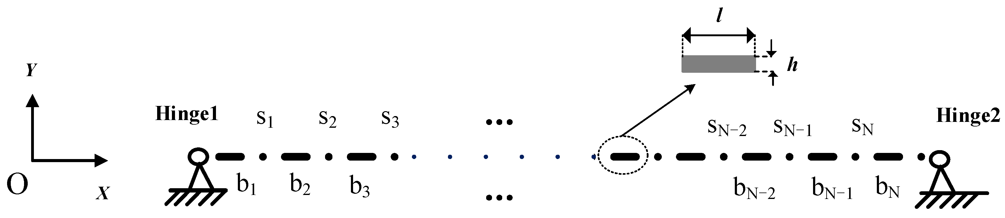
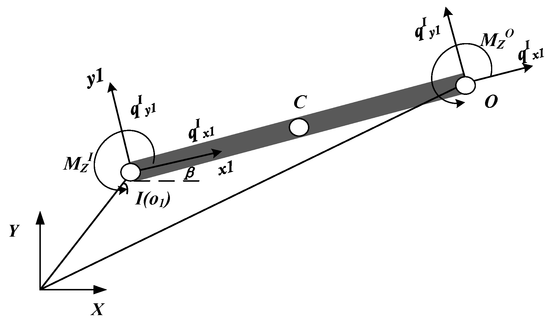
3.3. Transfer Matrix of the Flexible Link

In the flexible 3-PRR PPM, the flexible link can be discretized into multiple rigid body elements, which are connected by springs between segments using the wired segment method, as illustrated in Figure 5. Each rigid body element represents the inertial characteristics of the flexible link, while the elastic hinge describes the elasticity of the flexible body. By increasing the number of rigid body elements used to discretize the flexible link, a more accurate model can be achieved.

According to the linear MSTMM, the state vectors in modal coordinates at the input and output of the flexible link are $Z_I$ and $Z_O$, respectively, and the transfer equation can be expressed as:

$$Z_O=U_{b_N}{U}_{s_N}\cdots U_{s_1}{U}_{b_1}{Z}_I=U_L{Z}_I$$

(31)

where $U_b$ is the transfer matrix of the rigid body element and $U_s$ is the transfer matrix of the elastic hinge between the body element.

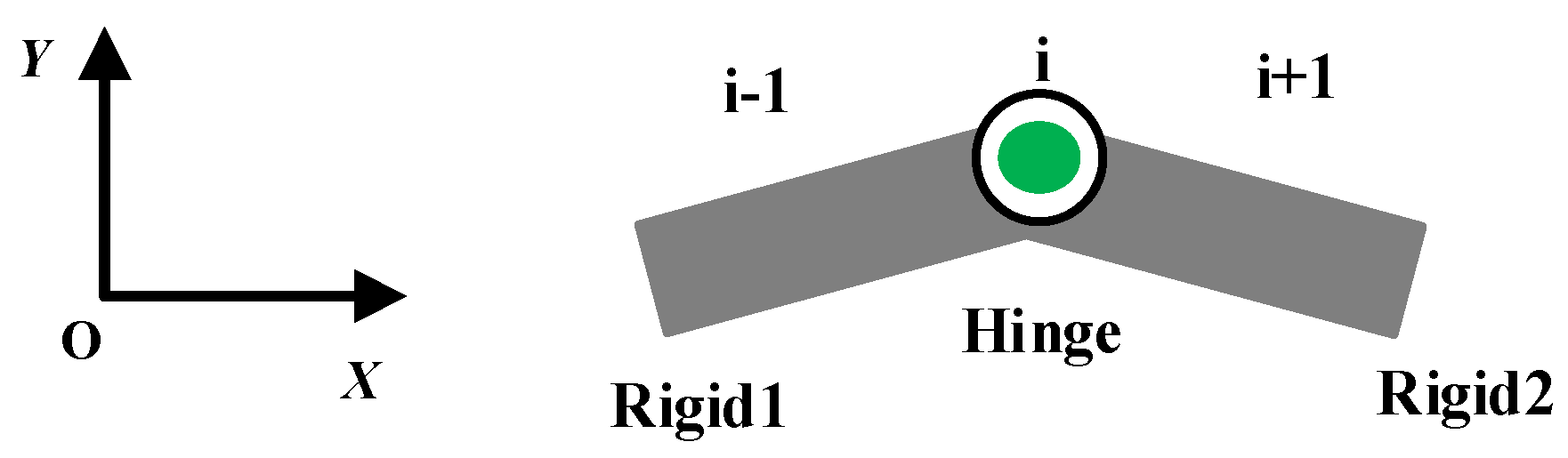
3.3.1. Transfer Matrix of the Elastic Hinge

To better approximate to the real situation, the modeling process takes into account both torsional vibrations and planar motions. As a result, the intersegment spring connecting two rigid bodies is defined as an elastic hinge composed of a torsion spring and a linear spring.

$$U_S=\left[\begin{array}{cccccc}1& 0& 0& 0& -\frac{1}{K_1}& 0\\ 0& 1& 0& 0& 0& -\frac{1}{K_1}\\ 0& 0& 1& \frac{1}{K_2}& 0& 0\\ 0& 0& 0& 1& 0& 0\\ 0& 0& 0& 0& 1& 0\\ 0& 0& 0& 0& 0& 1\end{array}\right]$$

(32)

In the transfer matrix of the elastic hinge, $K_1$ denotes the linear spring elasticity coefficient considering longitudinal deformation, while $K_2$ denotes the linear torsion spring elasticity coefficient:

$$K_1=\frac{EA}{∆l}=\frac{NEA}{L}$$

(33)

where $EA$ is the tensile stiffness and $∆l$ denotes the rigid body elements length,

$$M=EI\frac{{\partial }^2\omega }{\partial x^2}=EI\frac{\partial \delta }{\partial x}$$

(34)

$$K_2=\frac{M}{∆\delta }=\frac{EI}{∆l}=\frac{NEI}{L}$$

(35)

where $EI$ is the flexural stiffness and $M$ is the bending moment of the flexible link.

3.3.2. Transfer Matrix of the Rigid Element

Figure 6 illustrates the structure of a planar rigid body element, where the $x$-axis of the local coordinate system $o_1{x_{1}y}_1$ is along the neutral axis of the rigid body. The state vectors at the input and output are $Z_I \mathrm{a}\mathrm{n}\mathrm{d} Z_O$, respectively, and the transfer equation from the input point $I$ to the output point $O$ can be expressed as:

$$Z_O={\mathit{U}}_{\mathit{B}}{Z}_I$$

(36)

where:

$$U_B=\left[\begin{array}{cccccc}1& 0& -b_2& 0& 0& 0\\ 0& 1& b_1& 0& 0& 0\\ 0& 0& 1& 0& 0& 0\\ u_{\mathrm{4,1}}& u_{\mathrm{4,2}}& u_{\mathrm{4,3}}& 1& -b_2& b_1\\ m{\omega }^2& 0& {-m\omega }^2{c}_{c2}& 0& 1& 0\\ 0& m{\omega }^2& m{\omega }^2{c}_{c1}& 0& 0& 1\end{array}\right]$$

(37)

In the transfer matrix, ${u_{\mathrm{4,1}}=-m\omega }^2{(b_2-c}_{c2})$, ${u_{\mathrm{4,2}}=m\omega }^2{(b_1-c}_{c1})$, $u_{\mathrm{4,3}}=-{\omega }^2[J_1-m\left(b_1{c}_{c2}+b_2{c}_{c1}\right)]$, $\omega$ is the natural frequency of the parallel manipulator, and $J_1$ is the rotational inertia of the element with respect to $I$. The coordinates of the output point $O$ are denoted as $(b_1,b_2)$, and the coordinates of the center of mass $C$ are denoted as $(c_1,c_2)$.

3.4. Transfer Matrix of the Smooth Hinge

Figure 7 illustrates the structure of a smooth hinge, which is used to connect two bodies with free rotation. When a massless smooth hinge connects two rigid bodies at both ends, the input and output positions coincide, the internal forces are equal, and the internal moment is zero.

The state vector form of the planar hinge can be defined in a similar manner to Equations (4) and (5), and then from the literature [31], the transfer equation of the smooth hinge can be obtained as:

$$Z_O={\mathit{U}}_{\mathit{s}\mathit{h}}{\mathit{Z}}_{\mathit{I}}$$

(38)

where:

$$U_{sh}=\left[\begin{array}{cccccc}1& 0& 0& 0& 0& 0\\ 0& 1& 0& 0& 0& 0\\ -\frac{u_{\mathrm{4,1}}}{u_{\mathrm{4,3}}}& -\frac{u_{\mathrm{4,2}}}{u_{\mathrm{4,3}}}& 0& 0& -\frac{u_{\mathrm{4,5}}}{u_{\mathrm{4,3}}}& -\frac{u_{\mathrm{4,6}}}{u_{\mathrm{4,3}}}\\ 0& 0& 0& 1& 0& 0\\ 0& 0& 0& 0& 1& 0\\ 0& 0& 0& 0& 0& 1\end{array}\right]$$

(39)

$u_{\mathrm{4,1}}$,$u_{\mathrm{4,2}}$,$u_{\mathrm{4,3}}$,$u_{\mathrm{4,5}}$,$u_{\mathrm{4,6}}$ indicate the corresponding entries of the matrix in the next rigid body connected.

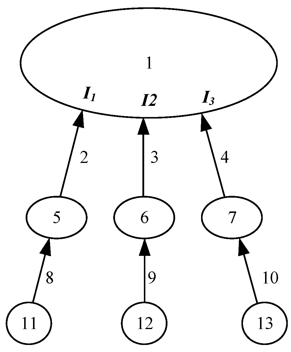
3.5. Overall System Transfer Equation

The flexible 3-PRR PPM consists of a mobile platform and three branch chain systems. Each chain system consists of a flexible link, a slider, and two smooth hinges. Three sliders are used as inputs to the system, and the center of the mobile platform is treated as the output. The components of the PPM are numbered and shown in Figure 8. The topology diagram in Figure 9 illustrates the transition relationship between state vectors, with each body element represented by a ‘◦’ and each hinge element and transfer direction represented by ‘→’. $I_j$ (j = 1,2,3) are the input of element 1 from elements 5–7.

In order to facilitate the analysis of the dynamics of the flexible 3-PRR PPM, the transfer matrix of the local coordinate system of the support chain system should be transformed to the same coordinate system with the mobile platform [33]. When the three flexible links are at angle ${\gamma }_j(j=\mathrm{1,2},3)$ with the $x$-axis of the mobile platform, the basic rotation matrix with respect to the coordinate system of the mobile platform is:

$$A_{sp}=\left[\begin{array}{cc}cos{\gamma }_j& sin{\gamma }_j\\ -sin{\gamma }_j& cos{\gamma }_j\end{array}\right]$$

(40)

Then, the transformation relationship of the same state vector in different coordinate systems is given by:

$$Z_I^{\prime }=R_{sp}{Z}_I Z_O^{\prime }=R_{sp}{Z}_O$$

(41)

where $R_{sp}$ denotes the directional cosine matrix.

$$R_{sp}=\left[\begin{array}{cccccc}cos{\gamma }_j& sin{\gamma }_j& 0& 0& 0& 0\\ -sin{\gamma }_j& cos{\gamma }_j& 0& 0& 0& 0\\ 0& 0& 1& 0& 0& 0\\ 0& 0& 0& 1& 0& 0\\ 0& 0& 0& 0& cos{\gamma }_j& sin{\gamma }_j\\ 0& 0& 0& 0& -sin{\gamma }_j& cos{\gamma }_j\end{array}\right](j=\mathrm{1,2,3})$$

(42)

Thus, the transfer equation of the three-branch chain system in the mobile platform can be obtained as:

$$\left\{\begin{array}{c}{{Z_4^{\prime }=R_{sp}\left({\gamma }_1\right)}_{}^{\mathrm{T}}U}_{I_{}}{R}_{sp}\left({\gamma }_1\right)Z_1\\ Z_8^{\prime }={{R_{sp}\left({\gamma }_2\right)}_{}^{\mathrm{T}}U}_{{II}_{}}{R}_{sp}\left({\gamma }_2\right)Z_5\\ Z_{12}^{\prime }={{R_{sp}\left({\gamma }_3\right)}_{}^{\mathrm{T}}U}_{{III}_{}}{R}_{sp}\left({\gamma }_3\right)Z_9\end{array}\right.$$

(43)

where $U_{I_{}}=U_4{U}_3{U}_2{U}_1$, $U_{{II}_{}}$=$U_8{U}_7{U}_6{U}_5$, $U_{{III}_{}}$=$U_{12}{U}_{11}{U}_{10}{U}_9$.

The overall transfer equation of the system can be expressed as:

$$U_p \left[\begin{array}{c}{Z}_4^{\prime }\\ \begin{array}{c}{Z}_8^{\prime }\\ \begin{array}{c}{Z}_{12}^{\prime }\\ Z_{G_{}}\end{array}\end{array}\end{array}\right]=U_P\left[\begin{array}{c}{{R_{sp}\left({\gamma }_1\right)}_{}^{\mathrm{T}}U}_{I_{}}{R}_{sp}\left({\gamma }_1\right)Z_1\\ \begin{array}{c}{{R_{sp}\left({\gamma }_2\right)}_{}^{\mathrm{T}}U}_{{II}_{}}{R}_{sp}\left({\gamma }_2\right)Z_5\\ \begin{array}{c}{{R_{sp}\left({\gamma }_3\right)}_{}^{\mathrm{T}}U}_{{III}_{}}{R}_{sp}\left({\gamma }_3\right)Z_9\\ Z_{G_{}}\end{array}\end{array}\end{array}\right]=O_{12\times 1}$$

(44)

The overall transfer equation, transfer matrix, and state vector equation of the system can be rewritten and organized in the following form:

$$U_{all}{{}_{12\times 24}Z}_{all}{}_{24\times 1}=0_{12\times 1}$$

(45)

where:

$${U_{all}=U}_P \left[\begin{array}{ccc}{{R_{sp}\left({\gamma }_1\right)}_{}^{\mathrm{T}}U}_{I_{}}{R}_{sp}\left({\gamma }_1\right)& & \begin{array}{cc}& \end{array}\\ & {{R_{sp}\left({\gamma }_2\right)}_{}^{\mathrm{T}}U}_{{II}_{}}{R}_{sp}\left({\gamma }_2\right)& \begin{array}{cc}& \end{array}\\ \begin{array}{c}\\ \end{array}& \begin{array}{c}\\ \end{array}& \begin{array}{cc}\begin{array}{c}{{R_{sp}\left({\gamma }_3\right)}_{}^{\mathrm{T}}U}_{{III}_{}}{R}_{sp}\left({\gamma }_3\right)\\ \end{array}& \begin{array}{c}\\ E\end{array}\end{array}\end{array}\right]$$

(46)

$$Z_{all}={[{Z_1}^{\mathrm{T}},{Z_5}^{\mathrm{T}},{Z_9}^{\mathrm{T}},{Z_{G_{}}}^{\mathrm{T}}]}^{\mathrm{T}}$$

(47)

3.6. Vibration Characteristics

3.6.1. Vibration Characteristics of Flexible Link

The flexible link is fixed in a flexible 3-PRR PPM with articulated ends, and the system boundary conditions can be expressed as:

$$Z_I={{\left[\begin{array}{cccccc}0& 0& {\Theta }_z& 0& Q_x& Q_y\end{array}\right]}^{\mathrm{T}}}_I$$

(48)

$$Z_O={{\left[\begin{array}{cccccc}0& 0& {\Theta }_z& 0& Q_x& Q_y\end{array}\right]}^{\mathrm{T}}}_I$$

(49)

We then substitute the boundary conditions into the transfer Equation (31).

$$∆=\left|\begin{array}{c}\begin{array}{ccc}{U_L}_{\mathrm{1,3}}& {U_L}_{\mathrm{1,5}}& {U_L}_{\mathrm{1,6}}\\ {U_L}_{\mathrm{2,3}}& {U_L}_{\mathrm{2,5}}& {U_L}_{\mathrm{2,6}}\\ {U_L}_{\mathrm{4,3}}& {U_L}_{\mathrm{4,5}}& {U_L}_{\mathrm{4,6}}\end{array}\end{array}\right|=0$$

(50)

Equation (50) is the system characteristic equation, which is a function of the natural frequency $\omega$, and $\omega$ has a solution for $∆=0$.

3.6.2. Vibration Characteristics of the Flexible Parallel Manipulator

By using the linear MSTMM, the overall transfer matrix of the whole system can be obtained by sequentially splicing the transfer matrices of the components in the flexible 3-PRR PPM. The characteristic equations of the whole system can be derived by substituting the boundary conditions, and its natural frequency can be determined by solving these equations.

For a specific position, a free vibration analysis is conducted on the flexible 3-PRR PPM. The state vector in the modal coordinates of the slider at the system inputs is provided as follows:

$$Z_{\mathrm{1,5},9}={{\left[\begin{array}{cccccc}0& 0& 0& {{\rm M}}_z& Q_x& Q_y\end{array}\right]}^{\mathrm{T}}}_{}$$

(51)

The output of the whole system is at the center of mass $G$ of the mobile platform, and since there is no external force acting on the mobile platform, it is free boundary so the terms $M_G$, ${q_x}_G,$ and ${q_y}_G$ are 0. Its state vector can be expressed as:

$$Z_G={{\left[\begin{array}{cccccc}X& Y& {\theta }_Z& 0& 0& 0\end{array}\right]}^{\mathrm{T}}}_{}$$

(52)

We then substitute Equations (51) and (52) for the boundary conditions into Equation (45) and eliminate the zero elements in the state vector $Z_{all}$ along with their corresponding column vectors in $U_{all}$. The system characteristic equation of the system is obtained as:

$${U_{all}^{\ast }}_{12\times 12}{Z_{all}^{\ast }}_{12\times 1}=0_{12\times 1}$$

(53)

where $U_{all}^{\ast }$ denotes the square matrix of the unknown variables in $U_{all}$ and $Z_{all}^{\ast }$ is the column matrix composed of the unknown variables in $Z_{all}$ Since $U_{all}^{\ast }$ is only related to the structural parameters of the system itself with the natural frequency $\omega$, $U_{all}^{\ast }$ has a non-zero solution and the determinant of $U_{all}^{\ast }$ needs to be zero.

$${∆}_{MSTMM}\left(\omega \right)=det{U}_{all}^{\ast }=0$$

(54)

The characteristic equation of the system is a function of $\omega$. It can be solved using the dichotomous method to obtain the natural vibration frequency of the flexible PPM system.

4. Numerical Simulation and Discussion

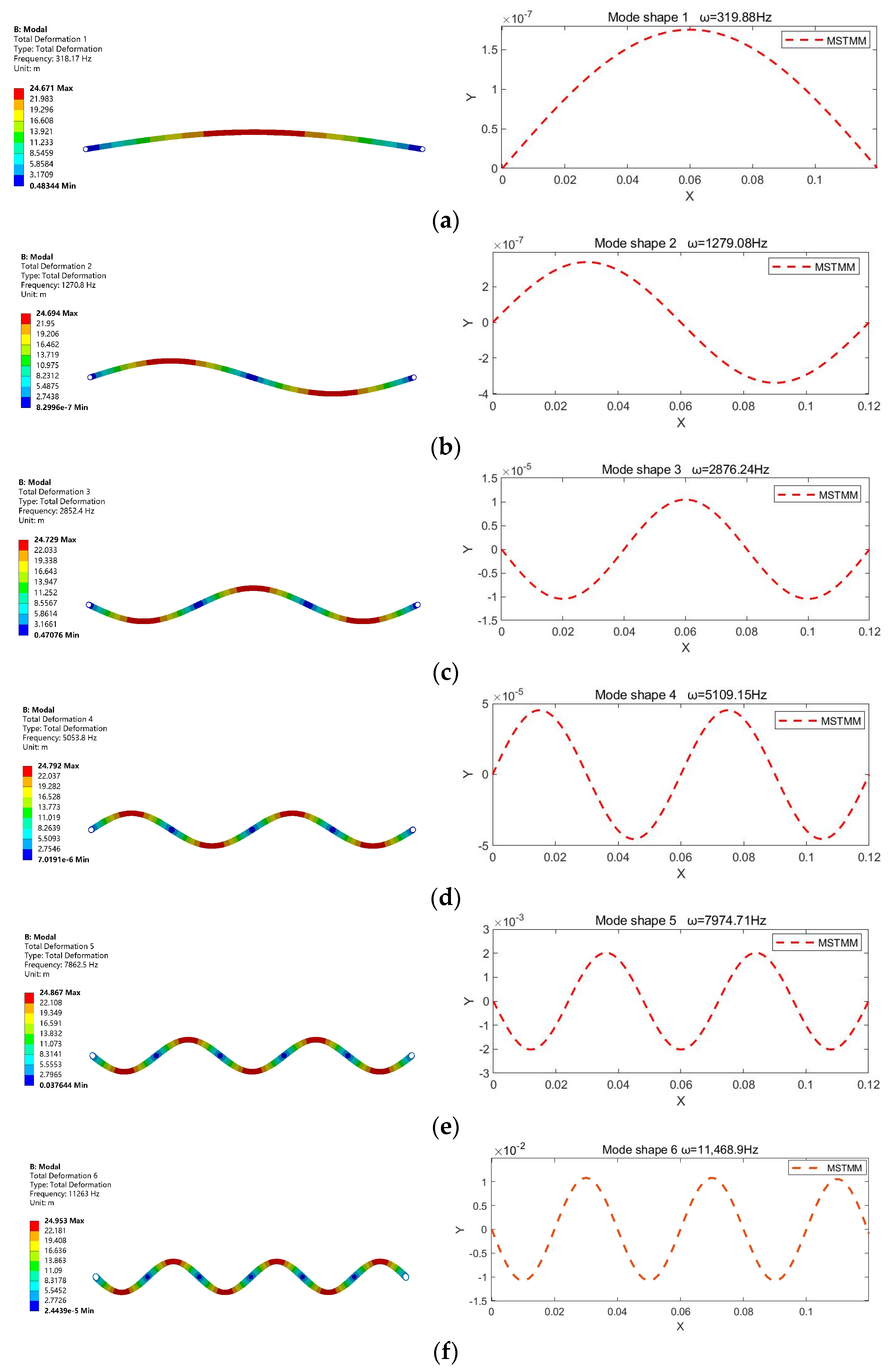
4.1. In-Plane Vibration of Flexible Link

To verify the accuracy and effectiveness of the proposed method, the vibration characteristics of the flexible link in the flexible 3-PRR PPM were numerically simulated using both MSTMM and FEM (Ansys Workbench). The parameters of the link were set as shown in

Table 1. Parameters of flexible link.

Symbols	Unit	Parameters
$\mathrm{L}=0.12$	[m]	Length of flexible link
$\mathrm{N}=400$	-	Number of split segments of flexible link
$E_1=7\times {10}^{10}$	[Pa]	Young’s modulus of flexible link
$\mathrm{b}\times \mathrm{h}=0.05\times 0.03$	[m]	Cross section parameters
${\rho }_1$ = 2740	[kg/m3]	Density of flexible link
$I_1$ = $\frac{1}{12}{m}_l{l}^2$	[kg.m2]	The inertia of the links

. The natural frequencies of the flexible link were calculated using the linear MSTMM. Furthermore, a simulation model was created in ANSYS Workbench, using the same structural parameters. The components were meshed with a hexahedral mesh, consisting of 4529 nodes, with a mesh size of 0.002 m.

The first six orders of natural frequencies and vibration shapes of the system in the plane obtained from linear MSTMM and FEM are given in

Table 2. Comparison of natural frequencies of flexible link.

Mode	$1\mathbf{st}$	$2\mathbf{n}\mathbf{d}$	$3\mathbf{r}\mathbf{d}$	$4\mathbf{t}\mathbf{h}$	$5\mathbf{t}\mathbf{h}$	$6\mathbf{t}\mathbf{h}$
MSTMM	319.88	1279.08	2876.24	5109.15	7974.71	11,468.9
FEM	318.17	1270.8	2852.4	5053.8	7862.5	11,263
Error(%)	0.57	0.64	0.82	1.08	1.41	1.79

and Figure 10, respectively.

The results demonstrate that the natural frequencies and mode shapes of the flexible link by MSTMM agree well with those obtained by FEM. This confirms that the proposed method is accurate for the description of flexible link.

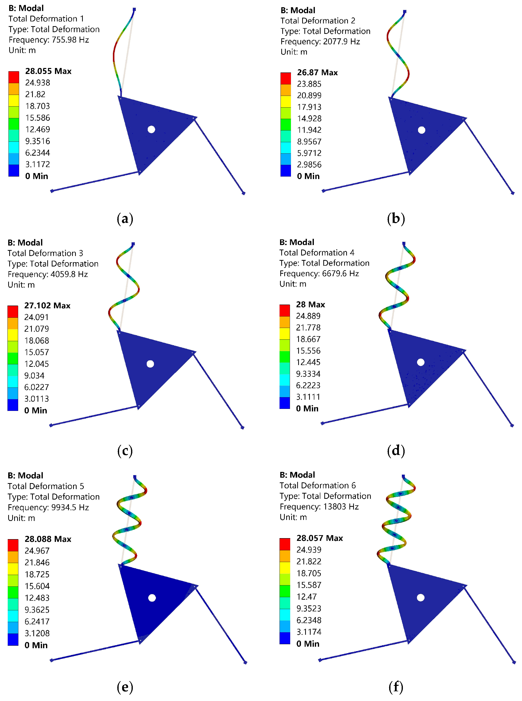
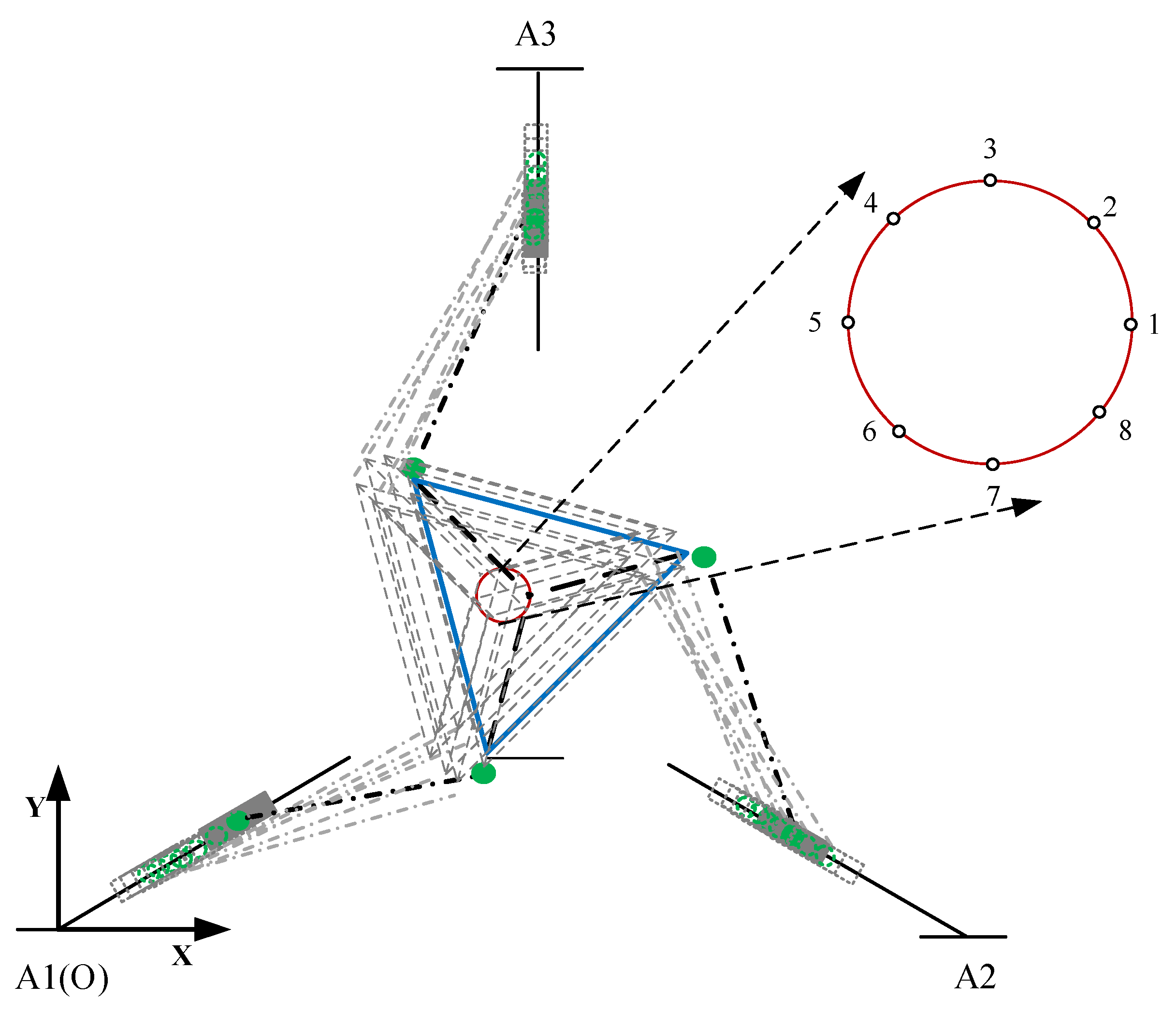
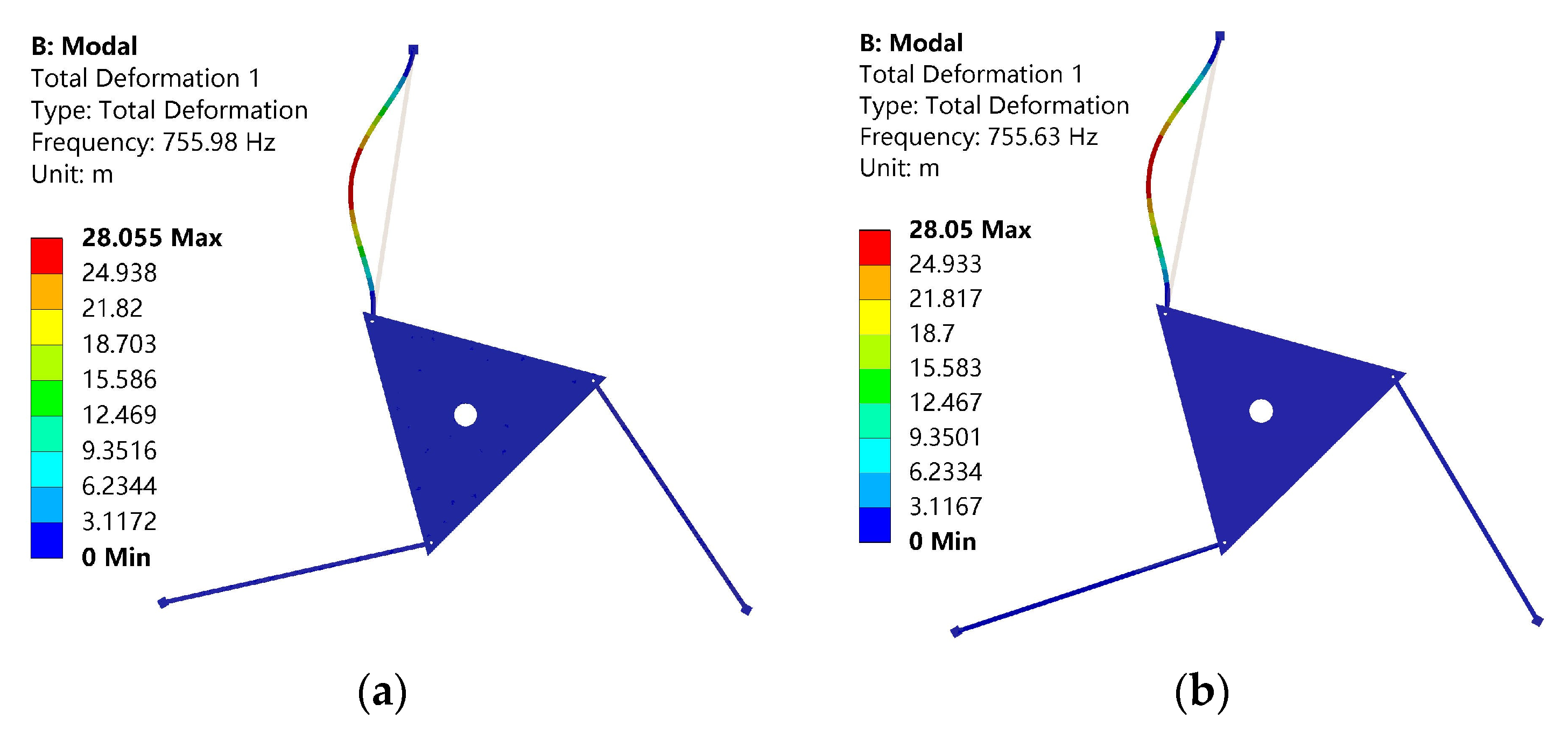
4.2. In-Plane Vibration of the Flexible 3-PRR PPM

To further verify the accuracy and effectiveness of MSTMM in modeling the flexible 3-PRR PPM depicted in Figure 2, the vibration characteristics of the parallel manipulator were simulated numerically using both linear MSTMM and FEM (Ansys Workbench), with identical structural parameters for the manipulator in both methods as listed in

Table 3. Parameters of the 3-PRR PPM.

Symbols	Unit	Parameters
$\mathrm{L}=0.12$	[m]	Length of flexible link
$\mathrm{N}=400$	-	Number of split segments of flexible link
$L_p=0.1$	[m]	Side of mobile platform
$m_s=5.7\times {10}^{-4}$	[kg]	Mass of slider
$E_1=7\times {10}^{10}$	[Pa]	Young’s modulus of flexible link
${m_p}_{}=0.2038$	[kg]	Mass of mobile platform
$\mathrm{b}\times \mathrm{h}=0.05\times 0.03$	[m]	Cross section parameters
${E_2}_{}=2\times {10}^{13}$	[Pa]	Young’s modulus of the mobile platform and slide
$\varnothing ={45}^o$	[deg]	Orientation of the platform
${\rho }_1$ = 2740	[kg/m3]	Density of flexible link
${\rho }_2$ = 7850	[kg/m3]	Density of mobile platform and slide
$I_1$ = $\frac{1}{12}{m}_l{l}^2$	[kg.m2]	Inertia of the links
$I_2=\frac{1}{3}{m}_p{L}_p^2$	[kg.m2]	The inertia of the mobile platform

. Moreover, to ensure consistency between the two methods, the component types and constraints between components were kept the same, especially in FEM, where a fixed-hinge joint was used to connect the flexible links to the mobile platform.

In the FEM simulation process, hexahedral meshes were used for the components, with the 3-PRR PPM divided into 55,993 nodes using a mesh size of 0.002 m. Additionally, the slider was fixed in place.

The natural frequencies of the system in the plane were obtained from linear MSTMM and FEM. Both natural frequencies and vibration shapes appear in three sequential groups and the differences in frequency values are small. In order to obtain better performance, we selected the first six order natural frequencies of the first link given in

Table 4. Natural frequencies of the flexible 3-PRR PPM.

Mode	$1\mathbf{s}\mathbf{t}$	$2\mathbf{n}\mathbf{d}$	$3\mathbf{r}\mathbf{d}$	$4\mathbf{t}\mathbf{h}$	$5\mathbf{t}\mathbf{h}$	$6\mathbf{t}\mathbf{h}$
MSTMM	737.69	2022.16	3958.45	6527.22	9719.89	13,528.04
FEM	755.98	2077.9	4059.8	6679.6	9934.5	13,803
Error(%)	2.42	2.68	2.49	2.28	2.16	1.99

, and Figure 11 shows the first six order mode shapes of the first link using FEM.

The results indicate that the errors of the first six orders of natural frequencies calculated by MSTMM and FEM are less than 2.68%. There is good agreement between the results obtained by the two methods, which demonstrates their accuracy. Thus, the MSTMM-based model effectively reflects the natural characteristics of the flexible 3-PRR PPM.

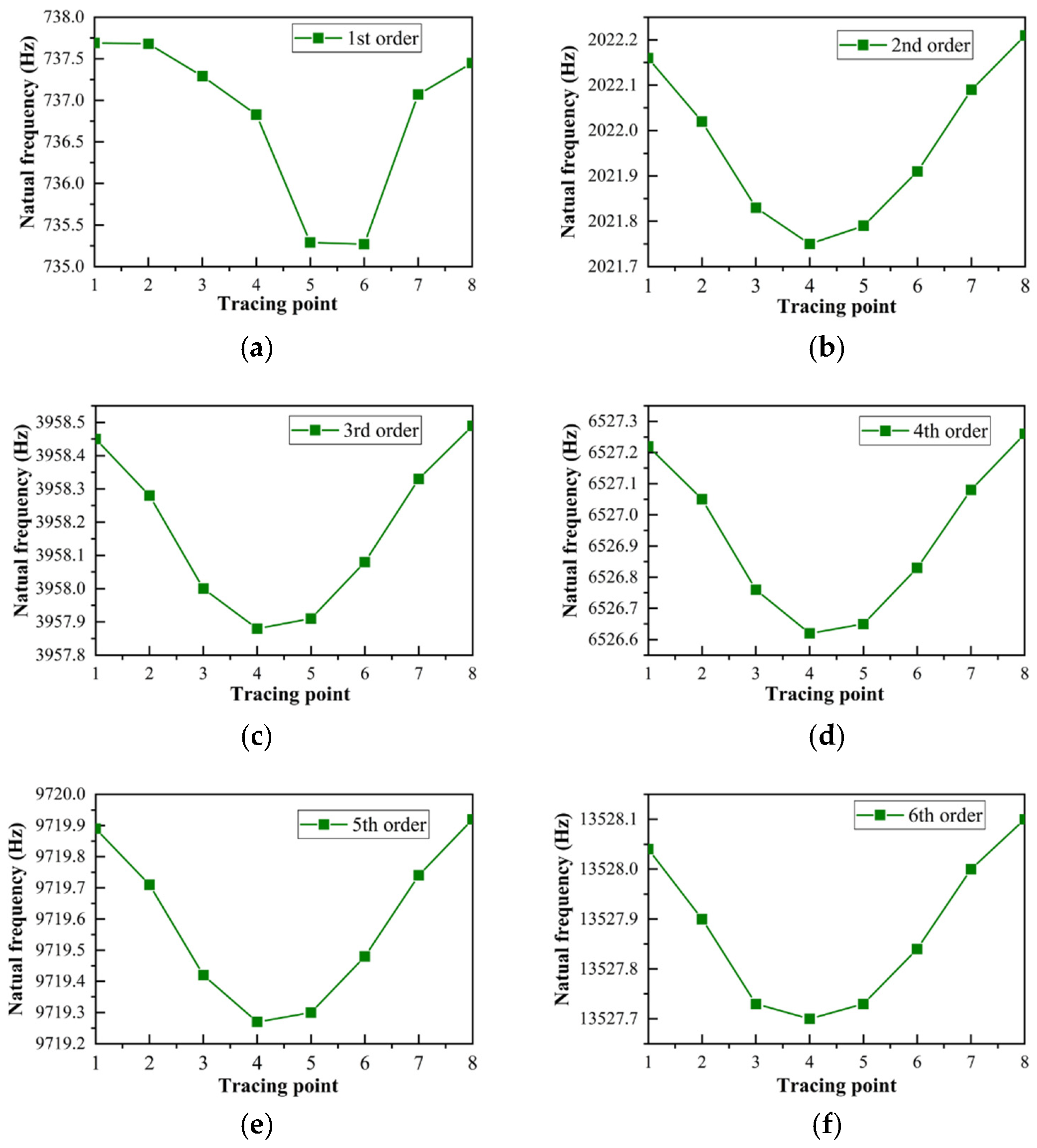
4.3. Analysis of the Vibration Characteristics of the Flexible Parallel Manipulator under a Specific Trajectory

To analyze the variation of natural frequencies of a flexible 3-PRR PPM under a specific trajectory, a circular trajectory with a radius of 0.015 m was given as the trajectory of the mobile platform. The angle $\phi$ between the mobile platform and the global coordinate system is fixed at 45°. This trajectory is defined as:

$$Xp=0.15+0.015\mathit{sin}\left(\pi t\right) (0\le t\le 2)$$

(55)

$$Yp=0.086+0.015\mathit{cos}\left(\pi t\right) (0\le t\le 2)$$

(56)

For easier analysis, we divided the circular trajectory into eight equidistant positions using the equipartition method. Then, we derived an approximate variation law by fitting the data. Figure 12 depicts the configurations of the parallel manipulator under the defined trajectory, and Figure 13 illustrates the first-order mode shapes obtained through FEM at the eight equidistant positions.

The first six orders of natural frequencies of the platform under different configurations are displayed in

Table 5. Natural frequencies of platforms under different configurations based on MSTMM.

Point	$\mathbf{Natural} \mathbf{Frequencies} {\mathit{f}}_{\mathit{k}} \left(\mathbf{Hz}\right)$
	$1\mathbf{s}\mathbf{t}$	$2\mathbf{n}\mathbf{d}$	$3\mathbf{r}\mathbf{d}$	$4\mathbf{t}\mathbf{h}$	$5\mathbf{t}\mathbf{h}$	$6\mathbf{t}\mathbf{h}$
1	737.69	2022.16	3958.45	6527.22	9719.89	13,528.04
2	737.68	2022.02	3958.28	6527.05	9719.71	13,527.90
3	737.29	2021.83	3958.00	6526.76	9719.42	13,527.73
4	736.83	2021.75	3957.88	6526.62	9719.27	13,527.70
5	735.29	2021.79	3957.91	6526.65	9719.30	13,527.73
6	735.27	2021.91	3958.08	6526.83	9719.48	13,527.84
7	737.07	2022.09	3958.33	6527.08	9719.74	13,528.00
8	737.45	2022.21	3958.49	6527.26	9719.92	13,528.10

through linear MSTMM numerical simulation. Figure 14 shows the variation curves of the first six orders of natural frequencies.

The results of the linear MSTMM numerical simulation indicate that the natural frequency of each order changes as the configuration of the flexible 3-PRR PPM changes. This suggests that the natural frequency of the platform will also vary with the configuration.

However, certain patterns can be analyzed through their variations. When the parallel platform changes its configuration along a specific circular trajectory, the first six orders of natural frequency exhibit a pattern of decreasing and then increasing. The changing trend from the second order to the sixth order is basically similar, and the second order is used as an example for analysis. As the position of the mobile platform is transformed from position 1 to position 8 according to the circular rule, the natural frequency from position 1 to position 4 shows a continuous decrease and reaches the minimum value at position 4. It then gradually increases and achieves the maximum natural frequency at position 8.

This rule illustrates the vibration characteristics of the flexible 3-PRR parallel manipulator and provides a crucial theoretical basis for subsequent research on dynamics optimization control.

5. Conclusions

This paper presents a linear MSTMM-based method for modeling and analyzing the dynamics of a flexible 3-PRR PPM. The overall transfer matrix of the system is obtained by sequentially splicing the transfer matrix of each element in this rigid-flexible multibody system. The vibration characteristics of the system are then calculated by solving characteristic equations according to boundary conditions. The natural frequencies obtained by MSTMM are compared with the results obtained using FEM to verify the accuracy and effectiveness. Finally, the natural frequencies under different configurations are analyzed using this method. The results show that the natural frequencies of the parallel manipulator keep changing with the position, and the trends of the first six orders are similar. This research provides the basis for the optimization of the dynamics of parallel manipulators.

Compared with the traditional method, this method has the following advantages:

(1)

There is no need for formulating and solving the global dynamics equations;

(2)

Even for complex multibody systems, the overall transfer equations are always of low order, with high computational efficiency and computational accuracy;

(3)

The principle is simple and efficient and can be easily extended to model and analyze other parallel manipulators containing flexible components.

References

1. Abo-Shanab, R.F. Dynamic modeling of parallel manipulators based on Lagrange–D’Alembert formulation and Jacobian/Hessian matrices. Multibody Syst. Dyn. 2020, 48, 403–426. [Google Scholar] [CrossRef]
2. Lu, H.J.; Rui, X.T.; Ma, Z.Y. Hybrid multibody system method for the dynamic analysis of an ultra-precision fly-cutting machine tool. Int. J. Mech. Syst. Dyn. 2022, 2, 290–307. [Google Scholar] [CrossRef]
3. Zhang, J.; Bi, L.; Wu, W.R. Reinforcement Learning-Based Parallel Approach Control of Micro-Assembly Manipulators. In Proceedings of the 2022 14th International Conference on Computer and Automation Engineering (ICCAE), Brisbane, QLD, Australia, 25–27 March 2022; pp. 25–30. [Google Scholar]
4. Alamdari, A.; Krovi, V. Design and analysis of a cable-driven articulated rehabilitation system for gait training. J. Mech. Robot 2016, 8, 051018. [Google Scholar] [CrossRef]
5. He, W.; Ouyang, Y.; Hong, J. Vibration control of a flexible robotic manipulator in the presence of input deadzone. IEEE. T. Ind Inform. 2016, 13, 48–59. [Google Scholar] [CrossRef]
6. Wang, D.; Cao, H.; Yang, Y. Dynamic modeling and vibration analysis of cracked rotor-bearing system based on rigid body element method. Mech. Syst. Signal. Process 2023, 191, 110152. [Google Scholar] [CrossRef]
7. Li, Y.B.; Wang, Z.S.; Chen, C.Q. Dynamic accuracy analysis of a 5PSS/UPU parallel mechanism based on rigid-flexible coupled modeling. Chin. J. Mech. Eng. 2022, 35, 33. [Google Scholar] [CrossRef]
8. Zhang, X.P.; Mills, J.K.; Cleghorn, W.L. Vibration control of elasto dynamic response of a 3-PRR flexible parallel manipulator using PZT transducers. Robotica 2008, 26, 655–665. [Google Scholar] [CrossRef]
9. Gao, H.J.; He, W.; Zhou, C. Neural network control of a two-link flexible robotic manipulator using assumed mode method. IEEE. T. Ind. Inform 2018, 15, 755–765. [Google Scholar] [CrossRef]
10. Piras, G.; Cleghorn, W.L.; Mills, J.K. Dynamic finite-element analysis of a planar high-speed, high-precision parallel manipulator with flexible links. Mech. Mach. Theory 2005, 40, 849–862. [Google Scholar] [CrossRef]
11. Li, Z.; Kota, S. Dynamic analysis of compliant mechanisms. In Proceedings of the International Design Engineering Technical Conferences and Computers and Information in Engineering Conference, Montreal, QC, Canada, 29 September–2 October 2002; Volume 5, pp. 43–50. [Google Scholar]
12. Wang, X.Y.; Mills, J.K. FEM dynamic model for active vibration control of flexible linkages and its application to a planar parallel manipulator. Appl. Acoust. 2005, 66, 1151–1161. [Google Scholar] [CrossRef]
13. Mahboubkhah, M.; Nategh, M.J.; Esmaeilzadeh Khadem, S. A comprehensive study on the free vibration of machine tools’ hexapod table. Int. J. Adv. Manuf. Tech. 2009, 40, 1239–1251. [Google Scholar] [CrossRef]
14. Liu, Z.; Yang, S.; Cheng, C. Study on modeling and dynamic performance of a planar flexible parallel manipulator based on finite element method. Math. Biosci. Eng. 2023, 20, 807–836. [Google Scholar] [CrossRef]
15. Karamanli, A.; Eltaher, M.A.; Thai, S. Transient dynamics of 2D-FG porous microplates under moving loads using higher order finite element model. Eng. Struct. 2023, 278, 115566. [Google Scholar] [CrossRef]
16. Chang, C.W.; Chen, Y.N.; Chang, H.C. Biomechanical comparison of different screw-included angles in crossing screw fixation for transverse patellar fracture in level walking: A quasi-dynamic finite element study. J. Orthop. Surg. Res. 2023, 18, 5. [Google Scholar] [CrossRef]
17. Al-Zahrani, M.A.; Asiri, S.A.; Ahmed, K.I. Free Vibration Analysis of 2D Functionally Graded Strip Beam using Finite Element Method. J. Appl. Comput. Mech. 2022, 8, 1422–1430. [Google Scholar]
18. Rui, X.T.; Wang, X.; Zhou, Q.B. Transfer matrix method for multibody systems (Rui method) and its applications. Sci. China. Technol. Sci. 2019, 62, 712–720. [Google Scholar] [CrossRef]
19. Rui, X.T.; Wang, G.; Lu, Y. Transfer matrix method for linear multibody system. Multibody Syst. Dyn. 2008, 19, 179–207. [Google Scholar] [CrossRef]
20. Rui, X.T.; U, O. Advances in transfer matrix method for multibody system dynamics. Adv. Mech. Eng. 2012, 42, 4. [Google Scholar]
21. Rui, X.T.; Zhang, J.; Zhou, Q. Automatic deduction theorem of overall transfer equation of multibody system. Adv. Mech. Eng. 2014, 6, 378047. [Google Scholar] [CrossRef]
22. Rong, B. Efficient dynamics analysis of large-deformation flexible beams by using the absolute nodal coordinate transfer matrix method. Multibody Syst. Dyn. 2014, 32, 535–549. [Google Scholar] [CrossRef]
23. Bestle, D.; Abbas, L.; Rui, X.T. Recursive eigenvalue search algorithm for transfer matrix method of linear flexible multibody systems. Multibody Syst. Dyn. 2014, 32, 429–444. [Google Scholar] [CrossRef]
24. Chen, G.L.; Rui, X.T.; Abbas, L.K. A novel method for the dynamic modeling of Stewart parallel mechanism. Mech. Mach. Theory 2018, 126, 397–412. [Google Scholar] [CrossRef]
25. Rong, B.; Rui, X.T.; Tao, L. Discrete time transfer matrix method for launch dynamics modeling and cosimulation of self-propelled artillery system. J. Appl. Mech. 2013, 80, 011008. [Google Scholar] [CrossRef]
26. Chen, D.Y.; Abbas, L.K.; Wang, G.P. The application of transfer matrix method for multibody systems in the dynamics of sail mounted hydroplanes system. In Proceedings of the International Design Engineering Technical Conferences and Computers and Information in Engineering Conference, Quebec City, QC, Canada, 26–29 August 2018; pp. 1–9. [Google Scholar]
27. Chen, D.Y.; Abbas, L.K.; Rui, X.T. Dynamic modeling of sail mounted hydroplanes system-part I: Modal characteristics from a transfer matrix method. Ocean Eng. 2017, 130, 629–644. [Google Scholar]
28. Rong, B.; Rui, X.T.; Tao, L. Theoretical modeling and numerical solution methods for flexible multibody system dynamics. Nonlinear. Dyn. 2019, 98, 1519–1553. [Google Scholar] [CrossRef]
29. Rui, X.T.; Zhang, J.S.; Wang, X. Multibody system transfer matrix method: The past, the present, and the future. Int. J. Mech. Sci. 2022, 2, 3–26. [Google Scholar] [CrossRef]
30. Wang, X.Y.; Mills, J.K. Dynamic modeling of a flexible-link planar parallel platform using a substructuring approach. Mech. Mach. Theory 2006, 41, 671–687. [Google Scholar] [CrossRef]
31. Si, G.N.; Chu, M.Q.; Zhang, Z.; Zhang, X.P. Integrating dynamics into design and motion optimization of a 3-PRR planar parallel manipulator with discrete time transfer matrix method. Math. Probl. Eng. 2020, 2020, 2761508. [Google Scholar] [CrossRef]
32. Si, G.N.; Chen, F.H.; Zhang, X.P. Comparison of the Dynamic Performance of Planar 3-DOF Parallel Manipulators. Machines 2022, 10, 233. [Google Scholar] [CrossRef]
33. Lu, H.J.; Rui, X.T.; Zhang, X.P. A computationally efficient modeling method for the vibration analyses of two-dimensional system structures using reduced transfer matrix method for multibody system. J. Sound Vib. 2021, 502, 116096. [Google Scholar] [CrossRef]
Figure 1. Topology diagram of a chain system in the transfer matrix method.
Machines 11 00505 g001
Figure 2. Configuration and coordinate system of 3-PRR PPM.
Machines 11 00505 g002
Figure 3. Mobile platform for 3-PRR PPM.
Machines 11 00505 g003
Figure 4. The slider model.
Machines 11 00505 g004
Figure 5. Discretization of the flexible link.
Machines 11 00505 g005
Figure 6. Model of rigid link.
Machines 11 00505 g006
Figure 7. Smooth hinge model.
Machines 11 00505 g007
Figure 8. MSTMM modal of the flexible 3-PRR PPM.
Machines 11 00505 g008
Figure 9. Topology figure of the flexible 3-PRR PPM.
Machines 11 00505 g009
Figure 10. Mode shapes of the flexible link: (a) first, (b) second, (c) third, (d) fourth, (e) fifth, and (f) sixth mode.
Machines 11 00505 g010
Figure 11. Mode shapes of the flexible 3-PRR PPM: (a) first, (b) second, (c) third, (d) fourth, (e) fifth, and (f) sixth mode.
Machines 11 00505 g011
Figure 12. Configurations of the platform under the designed trajectory.
Machines 11 00505 g012
Figure 13. The first-order mode shapes under different configurations: (a) first, (b) second, (c) third, (d) fourth, (e) fifth, (f) sixth, (g) seventh, and (h) eighth position.
Machines 11 00505 g013aMachines 11 00505 g013b
Figure 14. The first six natural frequencies under different configurations: (a) first, (b) second, (c) third, (d) fourth, (e) fifth, and (f) sixth mode.
Machines 11 00505 g014