1. Introduction
Innovations in the industry sector create the necessity for new paradigms, such as Industry 4.0 [
1,
2], Manufacturing 2.0, Smart Factories, and the Internet of Things (IoT). The way these models affect productivity is measured by their levels of flexibility, adaptivity, and traceability. The growth rate of this sector is also substantial since IoT technologies have become widespread with the purpose of facilitating communications. At the same time, the exchange of sensor measurements is feasible for further exploitation by utilising machine learning (ML) processes.
Production lines benefit from the modernization of manufacturing processes since new technologies can assist in quality diagnosis (QD) [
3]. Additionally, the application of simulation techniques optimizes key performance indicators. This results in improved efficiency when operating in real-time conditions. The goal of embracing new technologies in this industry sector is to increase product quality and, at the same time, reduce operational expenditures (OpEx) while maintaining or extending throughput.
ML in production lines has been used consistently during recent years. It is a process that increases the productivity and quality of the outcome [
4]. Many types of ML have been proposed to solve QD issues, such as (un- and semi-)supervised and reinforcement learning (RL) [
5]. The latter forms the core of the proposed Orion framework, presented in
Section 3 and evaluated in
Section 4. Some ML tasks that dominate the research in this industry field are regression, classification, data reduction, clustering, and anomaly detection. Additionally, ML is suited to solve NP-hard problems (where optimal solutions are not feasible since the complexity is exponential) in a heuristic manner [
6]. Heuristics solve these problems in real time, but the solutions are not optimal. The reduction in complexity compensates for this, however, given the nature of the computational problems.
ML techniques bring prediction capabilities [
7] that are necessary to avoid possible bursts of malfunctioning products. For example, if, in an early phase in the pipeline, some critical parameters are predicted to diverge from the acceptable value ranges during subsequent phases, an alarm is triggered for action to correct the process, avoiding unwanted output.
The main problem the current research confronts is the emergence of bursts of faulty products in the production line that require discarding. Values from sensors are consistently monitored, such as humidity, temperature and electrical currents. In the early phases of the pipeline, the personnel periodically record physical product parameters in a specific time interval. Therefore, the purpose is to correlate the two groups of values by utilizing RL techniques [
8,
9] and find which physical measurements have the highest impact on the sensor values. In this way, the personnel will be able to pay attention to the most critical measurements and avoid the future emergence of bursts of faulty products.
The main contributions of this research are:
The introduction of learning automata (LA) to manufacturing production lines;
A heuristic method is designed and used to prevent bursts of faulty products, and at the same time, provide real-time results for NP-hard computational problems. This work avoids resource-heavy conventional ML methods;
Adaptivity to changing environmental conditions (sensor values). The heuristic performs efficiently on every input dataset.
The content is organized as follows.
Section 2 presents the current state of this research field. Next, in
Section 3, the internal functionality of Orion is analyzed, and finally, a performance evaluation follows in
Section 4.
2. Related Research
Designing, implementing, and integrating an ML tool in a manufacturing process aims at increasing the quality of output components in a cost-effective manner. To ease the process, critical parameters must be captured for usage as input in the ML model. An artificial neural network (ANN) designed in [
10] uses as input the pulse frequency, cutting speed, and the laser power. Its task is optimization by predicting the non-linear functions that comprise laser cutting quality. It is shown by an evaluation that a set of optimized parameters can be obtained that improve the quality of the cutting process.
An interesting approach is presented in [
11,
12] for blockchain-based smart manufacturing quality control. It provides real-time monitoring using environmental sensors and reduces the latency, leading to decisions using blockchain. Additionally, predictive analysis assists the process of fault diagnosis, leading to cost savings.
Zero-defect manufacturing (ZDM) is a concept that, when applied, tries to minimize product defects during the production phase by delivering output within the predefined specifications. It decreases costs by discarding the unqualified products from further processing in the line. This is also one of the main goals of the proposed solution named Orion (analyzed in
Section 3). In this work [
13], a predictive quality control method in a multi-stage manufacturing process (MMP) aiming at ZDM is presented. By considering the correlations between different measurements, a deep supervised network is built to predict quality characteristics. The assembly line process is optimized by a genetic algorithm network.
In a production line, the generation of flat surfaces requires machining processes, such as face milling [
14]. The main parameter that is considered by international standards for measuring the quality of surfaces is roughness. When tool wear increases, it deteriorates. Deviations of surface roughness can be predicted by utilising ML methods. Three parameters that are correlated to surface roughness can be estimated, i.e., maximum tool wear, machining time, and cutting power. ML methods, such as random forest (RF), standard multilayer perceptrons (MLP), regression trees, and radial-based functions, are evaluated for this purpose. RF showed the highest accuracy, followed by regression trees. Similarly, deviations can be predicted by Orion by utilizing RL. Models to predict the in-process thickness during the steel plate rolling milling machine phase are presented [
15]. By applying these, the thickness needed to produce high-quality steel plates is reduced, along with the cost. To achieve this goal, clustering and supervised learning algorithms are utilized.
An interesting approach to minimizing sensor usage is to exploit audio signals [
16]. With this method, only a single sensor is required, as is a method to remove noise. Dimensionality is reduced by an extended principal component analysis. The classification of tool wear conditions is achieved with high accuracy in the results.
A combination of cluster analysis and supervised ML, targeting product state data during manufacturing from sensor measurements, is utilised for handling complexity (which is also a performance goal of Orion) and high dimensionality [
17]. Support-vector machine (SVM) is the ML model of choice in this case due to its accuracy and performance with the high dimensionality of the data. To achieve this goal, the manufacturing process sequence is limited to a well-known set of states and forms the basis for a hybrid approach relying on both process monitoring and control. Similarly, a data-driven predictive maintenance system [
18] that utilizes ML methods is presented. Its purpose is to detect potential failures early on in the process. Sensor data are stored in a cloud system database where distributed systems access them using Internet of Things (IoT) technologies to convert them into single data types. Next, it uses ML algorithms to detect signals of potential errors. The output is the estimated remaining time before failure.
A product’s dimensional variability is the problem this work [
19] tries to confront by utilising ML techniques in complex multistage manufacturing processes. Several classifiers were trained and tested with the purpose of predicting manufacturing defects on the assembly line of the automotive industry. According to the demonstrated results, non-linear models such as XGBoost and RFs show efficient performance related to quality control. Therefore, defects and deviations are addressed in a timely fashion, minimizing production costs. Manufacturing defects are also predicted by Orion.
In a similar vein [
20], methods depending on image inspection are those using recurrent neural networks such as MLP. A comparison took place with conventional ML methods, such as decision trees (DT), RF, k-nearest-neighbors, SVM, naïve Bayes, and logistic regression, for the detection of anomalies. Conclusion are drawn, with the RF having the best recall, accuracy, precision and F1 score. In this study, conventional ML methods are superior to MLP.
Another anomaly detection approach [
21] consists of an autoencoder, a deep neural network to produce the anomaly score, and a discriminator to automatically detect anomalies. Some key traits are the support of human operators without an advanced computer science background, the short training time that is required, and finally, the improvement of other methods’ precisions and accuracies. A decision support mechanism [
22] using an anomaly detection algorithm for multi-agent systems was developed for the purposes of facilitating autonomous production execution and process optimization. It is a manufacturing execution system with ML embedded in its computational logic.
Product defects are detected using machine vision [
23]. This model also predicts the most suitable parameters of processes in the production line in order to obtain defect-free products. The depicted results aid in choosing the most appropriate ML models to boost performance. It achieves 95% accuracy within the acceptable time frame. Failures are also analyzed and exploited [
24] in order to train the utilized model and assist in the prediction of future defects. Optical inspections related to the physical dimensions are used to detect various physical defects of the products in the line. This is the corresponding procedure of Orion, but it is carried out manually by the personnel in that case. Next, classification follows from the detected defects according to specific patterns and geometries. When defects are confirmed, they are added to a library for future training.
ML techniques, together with edge cloud computing, are utilised to investigate a solution of predictive-based quality inspection for manufacturing purposes [
25]. This is a holistic approach that is based on target-oriented data acquisition, processing, and modeling, and it is suited for implementation in the IT plant infrastructure. Quality inspection takes place for finished or semi-finished products in the manufacturing line. The proposed approach ranges from systematic data selection to the training of predictive models, as well as to implementation and subsequent integration.
ML techniques, PLCs (programmable logic controllers), cloud services, and AI algorithms serve the purpose of classifying defective products in a manufacturing line [
26]. PLCs comprise the main logic for controlling power circuits. This system is evaluated by training the network on casting product data. It is shown in the results that the classification of input images with high accuracy and real-time speed is achieved. Classification is also utilized [
27] by deep learning methods with images of line products to separate the defective products and guide them out with the assistance of PLCs. This study shows that detection based on images can also perform well on more complex products. The quality control process can be implemented without powering off the assembly line.
A high-level approach (in contrast to Orion) to a product quality monitoring system with smart factory technology is presented [
28]. Smart and intellectual system design principles are incorporated so as to provide effectiveness in real applications. The design method that was used is named Smart Manufacturing Systems Engineering. Specifically, it is focused on integrating smart manufacturing procedures into the phase of defining the system’s design. In a similar vein, another study [
29] proposed a full manufacturing proposal based on cognitive intelligence and edge computing. It includes methods to efficiently utilise interactions, multimodal data fusion, and automatic production during the manufacturing process. Additionally, the performance of a traditional system is analyzed in comparison to the proposed method in order to evaluate the performance according to instruction calls and production efficiency.
The aforementioned examples are indicative that the research in QD (
Table 1) during the production pipeline is dominated by ML tools [
4,
30]. All shown results explain and justify the extensive usage of learning and adaptive techniques.
3. Orion QD Framework
In this section, the proposed solution is presented, namely Orion. It is a scientific framework for integration into the production line, for controlling product quality, and at the same time, for reducing operational expenditures. It can be applied to manufacturing lines to keep track of the quality of products according to manually recorded measurements (regressands) in correlation with the corresponding sensor values (regressors). The latter consists mainly of environmental parameters, such as temperature, humidity, and electrical currents, that can be automatically detected by specialized sensors. Personnel, on the other hand, measure important physical product parameters such as dimensions, weight, and surface roughness. According to these measurements, and considering the sensor values as well, Orion will be able to predict future deviations from the acceptable value ranges for the physical parameters comprising the product quality.
Orion is an innovative framework for QD that heuristically solves the computational complexity issues most ML techniques face. LA [
31] have been used in the past in other fields of computer science, e.g., in networking [
32]. To the knowledge of the authors, LA have not been used before in a production line. They can provide a short-term quality estimation window with a low execution time, which is important to save OpEx and guarantee consistent product quality. Additionally, LA demonstrate the ability to adapt to runtime changes by exploiting feedback from the environment [
33]. This is a trait that provides stable performance without dependence on specific datasets.
The purpose of applying Orion to a production line is to be able to predict a possible burst of defective products. Since this burst takes place at a future time, it is avoided, thus saving production costs and controlling quality. In the context of Orion, a defective product is defined as one having its measured physical parameters outside of the acceptable range of values. For example, if the surface roughness is allowed in the range [0–10%], every product with a higher value is considered defective and must be discarded from the production line. The same logic applies to the physical dimensions as well.
The innovative nature of Orion consists of:
A low level of complexity for resource-heavy computational problems. This makes Orion suitable for real-time execution.
An implementation suitable for embedded devices in the production line.
Fast adaptivity to varying input measurements. Orion performs well with every input dataset.
3.1. Activity
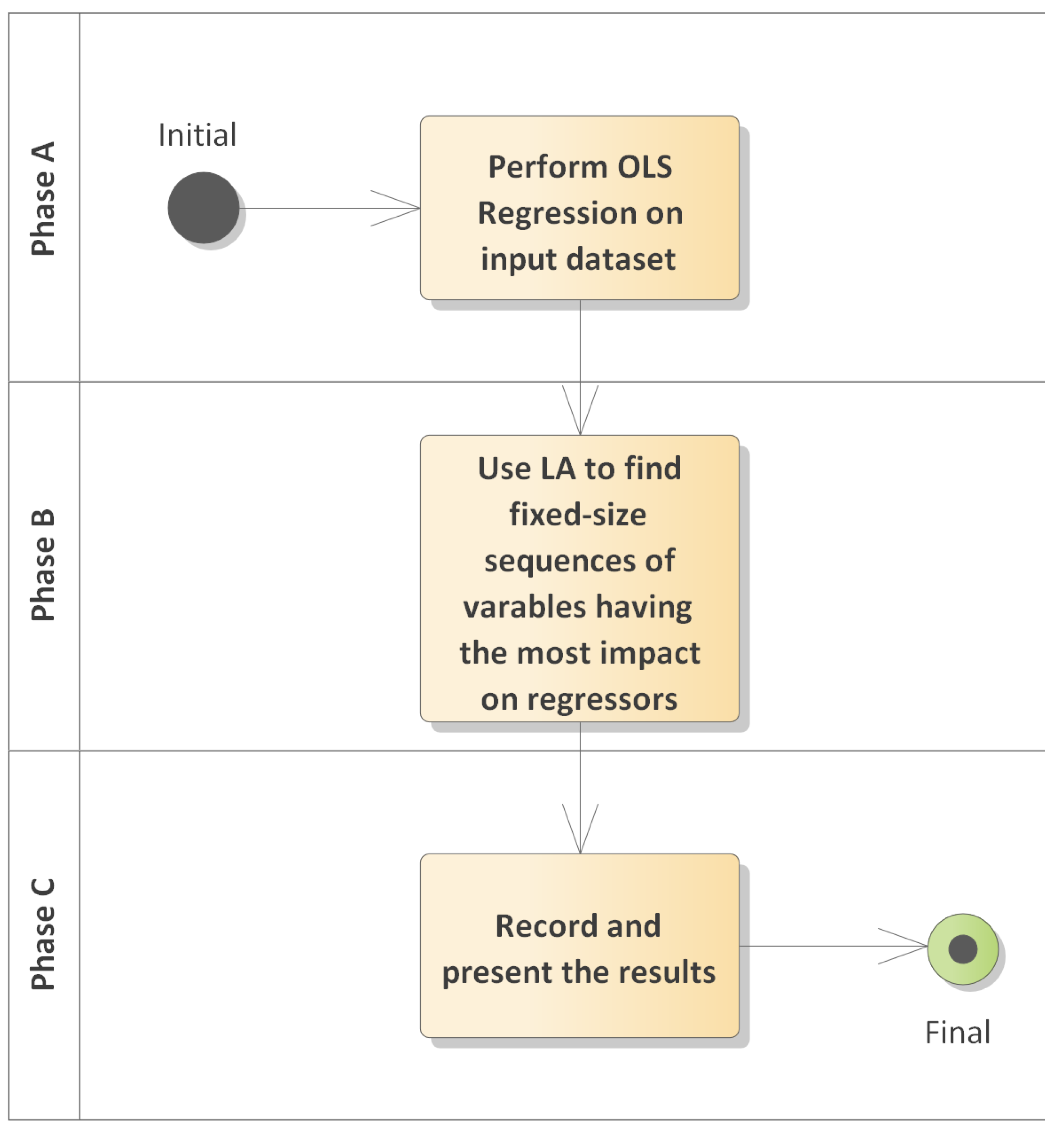
The activity of Orion consists of three phases, as depicted in
Figure 1. First, it performs ordinary least squares (OLS) regression [
34] on the regressands and stores the results. Linear regression is referred as OLS since it emphasizes the minimization of the squared deviations from the regression line. It is used from
statsmodels.api of Python. Second, it utilises LA to find sequences of regressands having the most impact on regressors, and finally, there exists the last phase, where results are stored in a suitable form to draw conclusions from. Each phase provides its output as input to the next phase in the chain.
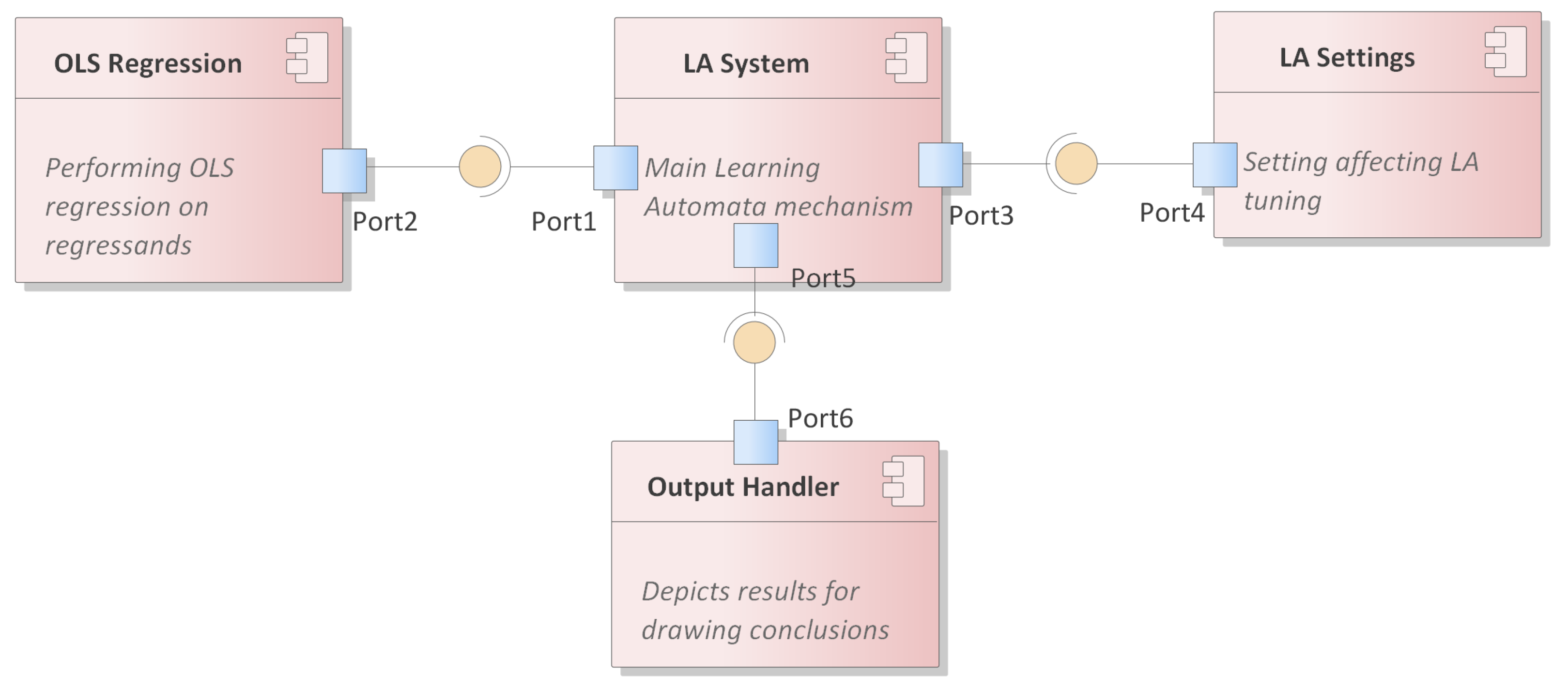
Depicting the framework with the components it consists of (as in
Figure 2), the
LA System lies at the core, obtaining input from two other components, i.e., the
OLS regression and the
LA settings. When it converges to a sequence of regressands, it provides input to the output handler component, where conclusions are depicted for the non-tech savvy work force in the production line.
OLS is used for every regressand to find the number of regressors having the most impact for minor value fluctuations of the former. The widely used threshold for
p-values [
35] in such cases is 5%. That is, if the regressor’s
p-value is within the range [0, 0.05], it is considered to have a high impact when value variations of the regressand occur. The functionality of this component concludes when the mapping of every regressand to the number of regressors with
p-values lower than the threshold is collected and stored for usage as input in the LA system component.
3.2. LA System Component
The
LA system component represents the core of Orion’s adaptivity. It is based on RL logic to find sequences of regressands having the most impact on regressors. This is an NP-hard computational problem (all available fixed-size combinations of variables that produce the highest impact sum) to solve [
36], so a heuristic method such as this (implemented with LA) is required to provide practical results in real time for a large number of regressands.
LA exploit feedback that results from every possible taken action in order to converge on the one action which is highly evaluated according to predefined criteria. For example, in case there are three available actions to take, all of them are correlated to a probability number (summing to 1). Initially, one of these actions is chosen randomly, and according to the feedback that is returned from the resulting system state, its correlated probability number either increases or remains unaltered. The numbers of the other two actions are adjusted accordingly, so the total sum always equals 1. The LA converge to the action that returns the higher feedback after a number of iterations.
In a state of convergence, the highly evaluated action reaches a probability value close to 1, while the others take values close to 0. This is interpreted as the final stage to reach to draw conclusions. In subsequent iterations, this action will be chosen with higher probability than the others. Since the feedback from the environment may change considerably at any time, subsequent iterations may push the LA to converge to a different state. This ability to adapt to the varying input dataset renders the mechanism valuable in a consistent operational state.
In the context of a manufacturing environment, this RL mechanism is exploited by the proposed Orion QD solution to find the sequence of human-measured variables in the first stage of the production line, having a high impact on the sensor values in a later stage. The latter group of values depicts the environmental conditions.
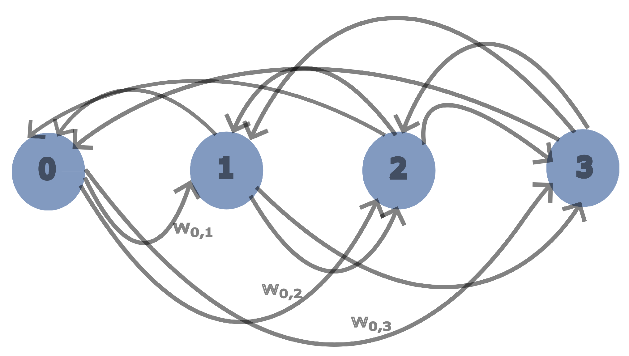
To find the sequence of regressands with the most impact on the product quality, a directional graph structure (
Figure 3) is created, with all the regressands as nodes. The node relationship is one to all. The purpose is to find a sequence of nodes with a predefined length (in hops) that returns the highest evaluation number concerning the impact on the regressors. An LA is placed in every node of the directional graph with the purpose of evaluating its neighbor connections. In the example of
Figure 3, if a sequence with size 3 is required to be found, an iteration occurs multiple times, initiating from all nodes until 3 of them are traversed. According to the feedback from the last node, all intermediate nodes adjust their weights to the other one-hop connections. This way, edges leading to efficient paths have weights that subsequent traversals will prefer. After a number of iterations, the LA at each node converge and point to the neighbor that leads to the preferred path.
Starting by iterating sequentially throughout the nodes, a traversal occurs for a fixed number of hops that is equal to the amount of regressands to find. The last node returns feedback to the initial node, as well as to all intermediate ones, about the specific path evaluation. According to this value, all path nodes adjust their probabilities pointing to all neighbors using Formulae (
1) and (
2). For each path node, the first of these formulae subtracts a quantity from all neighboring nodes that are not part of the path, and by using the second formula, the sum of these quantities is added to the node participating in the path. All probabilities of reachable neighbors to a path node always sum to 1.
In Formula (
1),
L is used to handle the problem of convergence speed over the accuracy of the estimation. Different values favor speed over accuracy and vice versa. The value of
a is a guard in this formula to prevent probability values from reaching a zero value, leading to starvation. Additionally,
is the feedback,
p is the current probability of node
j, and finally,
k is the time slot.
The highest cost G value that is calculated from the neighboring nodes in Formula (
4) is used to pick up the next node during traversal.
T is the current time slot, and
is the corresponding time slot when neighbor
i was last chosen. The variable
p is the estimated probability value for neighbor
i, and
l is used as the weight. For efficiency, the weight is multiplied by 10 and floored to represent
l.
M is the number of neighbors. The G equation ensures that neighbors with low-probability numbers will still have a chance for pick up, even though more scarcely, to avoid starvation.
Calculating the feedback value
that is used by the LA to adapt after each iteration initially requires setting weights between each node pair. Formula (
3) is used for this purpose. Specifically, the weight between node pair AB is inversely equal to the sum of regressors having a
p-value of less than 0.05 for regressand A, plus the corresponding sum for regressand B. Finally, the defined feedback by Orion equals 0 if the current path-weight is higher than the average of the previous path-weights (in previous iterations); otherwise, it is equal to the percentage increase if it is less than the average. The purpose of this is to converge near the lowest path-weight sum.
3.3. LA Settings Component
LA require a set of settings to assist in adapting to the runtime environment. Tuning these settings impacts the convergence speed, and at the same time, the proximity percentage to the optimal solution.
Values from
Table 2 are provided to the LA core during the initialization phase. Finally, the output handler is a component that provides the ability to present, in a human-readable form, the results that follow in
Section 4.
4. Results
The process of finding the sequences of dependent variables impacting the output sensor values is simulated, along with the OLS regression upon the provided dataset from Factor Ingeniería y Decoletaje S.L. This dataset consists of 13 automated sensor measurements, i.e., the temperature of 6 motors and the coolant oil, the total power consumption, values of three currents, and finally, the environmental temperature and humidity. On the production line, the manually recorded measurements by the personnel consist of 18 variables related to the physical product’s dimensions, surface roughness, and weight.
Initially, each LA’s available choice has a probability equal to 1 divided by the sum of choices. In this way, all choices start under the same conditions. Parameter
a has a value of 0.0001.
L is equal to 0.15, which is a value that provides an acceptable trade-off between convergence speed and accuracy in this environment. Next,
l as an integer value. To produce this value, the edge’s weight is floored to the integer that represents the proximity to the maximum edge weight value. Finally, the simulation time is slotted, so
T and
R(i) of Formula (
4) hold values that increase with the same step.
The main engine and the LA were implemented in C++20 using the Clang 14 compiler. The OLS regression was run in Python 3.9. Both of these were performed on an ARM macOS 13.x.
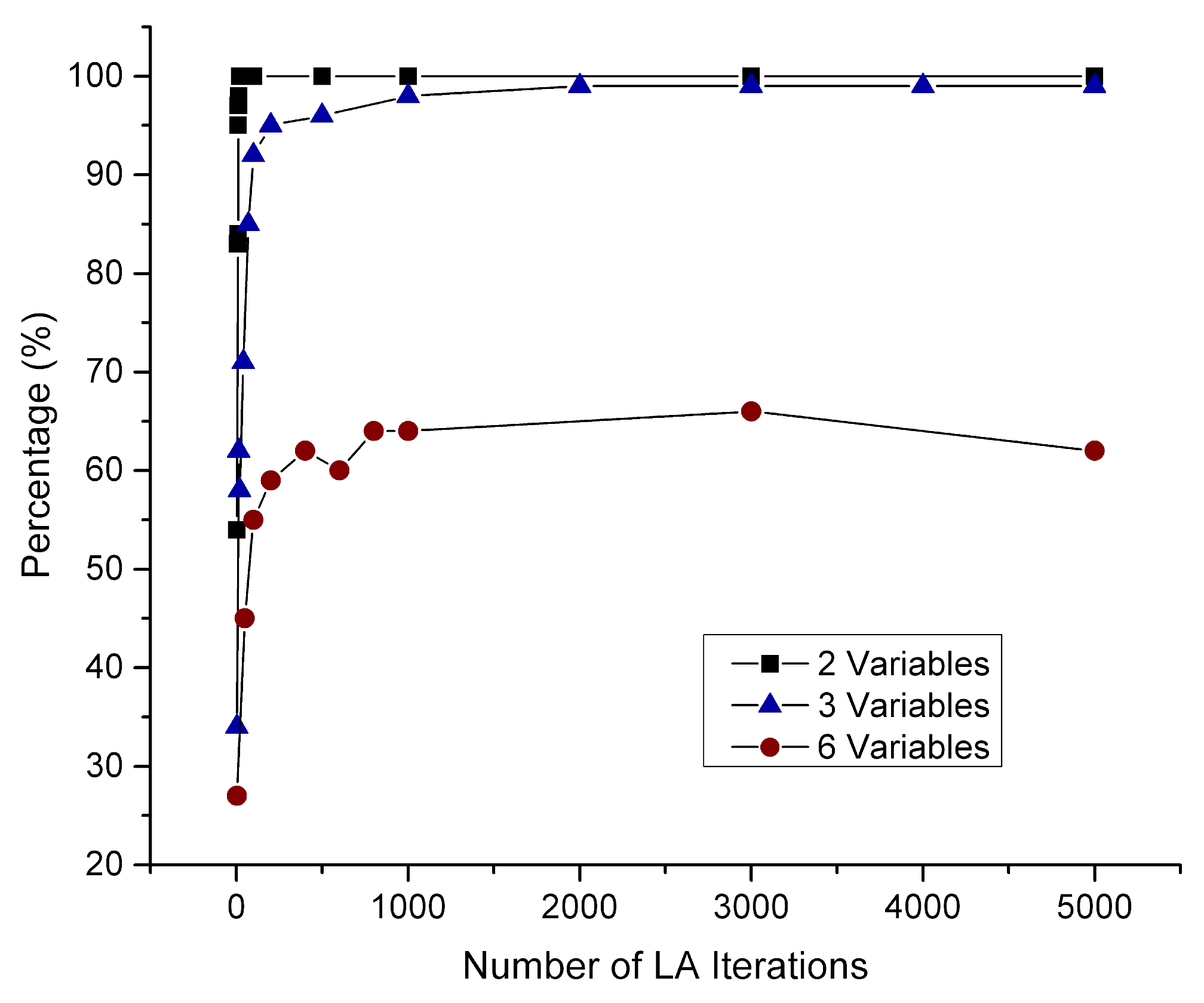
Figure 4 depicts the impact the number of LA iterations have on the percentage of executions that yielded the highest
p-value sum within the dependent variable sequence. Each regressand correlates to a number of regressors having
p-values smaller than the threshold of 0.05 (from the literature). This correlation is the
p-value sum for a regressor, and when it increases, the impact on the regressands is higher. When the number of the latter in the sequence is small, few LA iterations are required for convergence to the highest
p-value sequence. As the number of variables in the sequence increases, more LA iterations are required for convergence. In the cases of 2 and 3 variables, 2000 more iterations are required for the latter to increase its percentage from 90% to 99%. In the case of 6 variables, 60% of executions yield the optimal results.
In
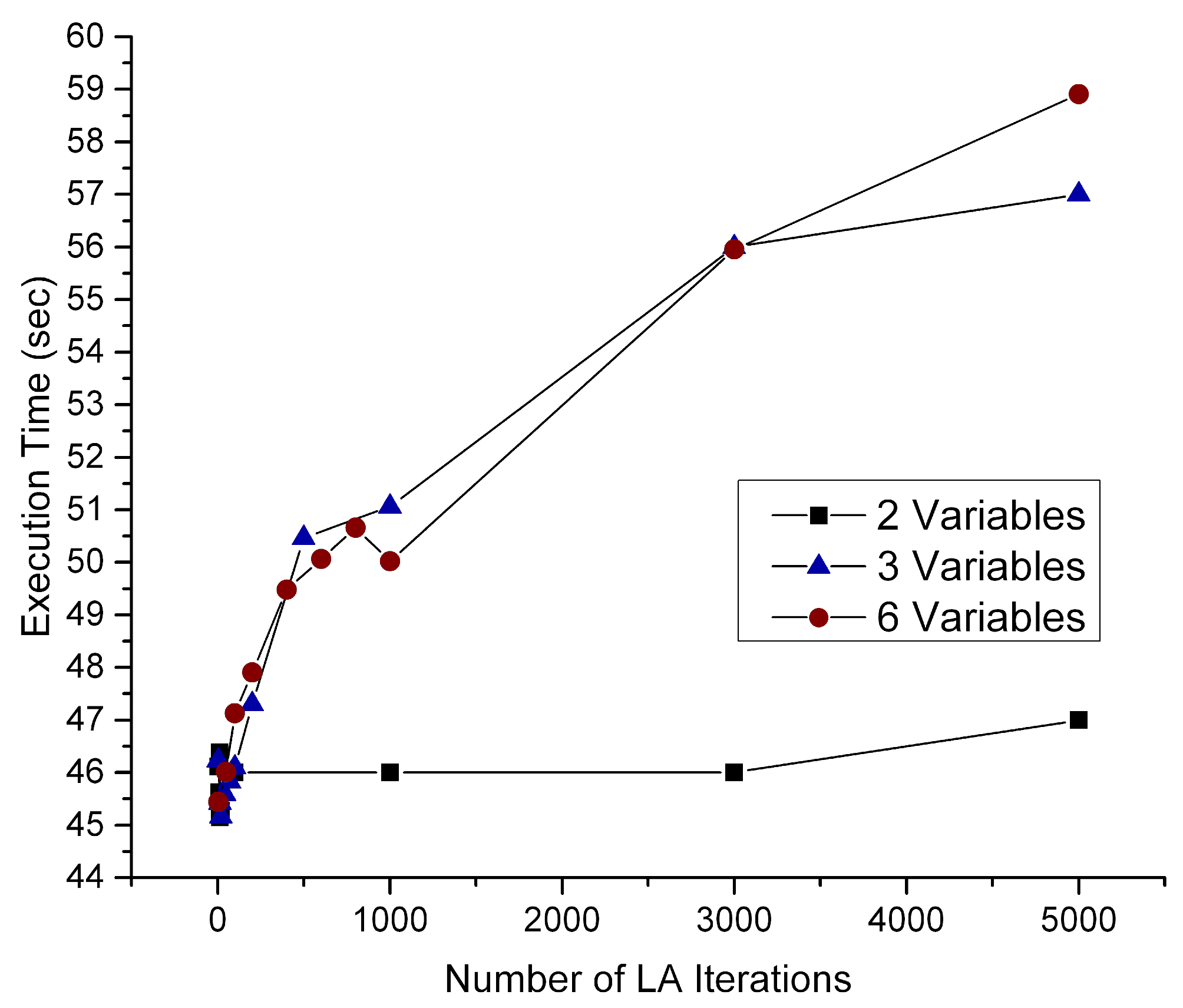
Figure 5, the impact the LA iterations have on the execution time is depicted. As the number of iterations increases, there is almost a linear correlation with the execution time for finding the efficient variable sequence. A smaller sequence size requires less execution time. In the case of just two regressands, the computational process is simple, so there is a small increase in execution time. The time windows increase from 46 s to 59, which is very low in comparison to the increase in LA iterations to 5000. This renders the algorithm able to scale.
In
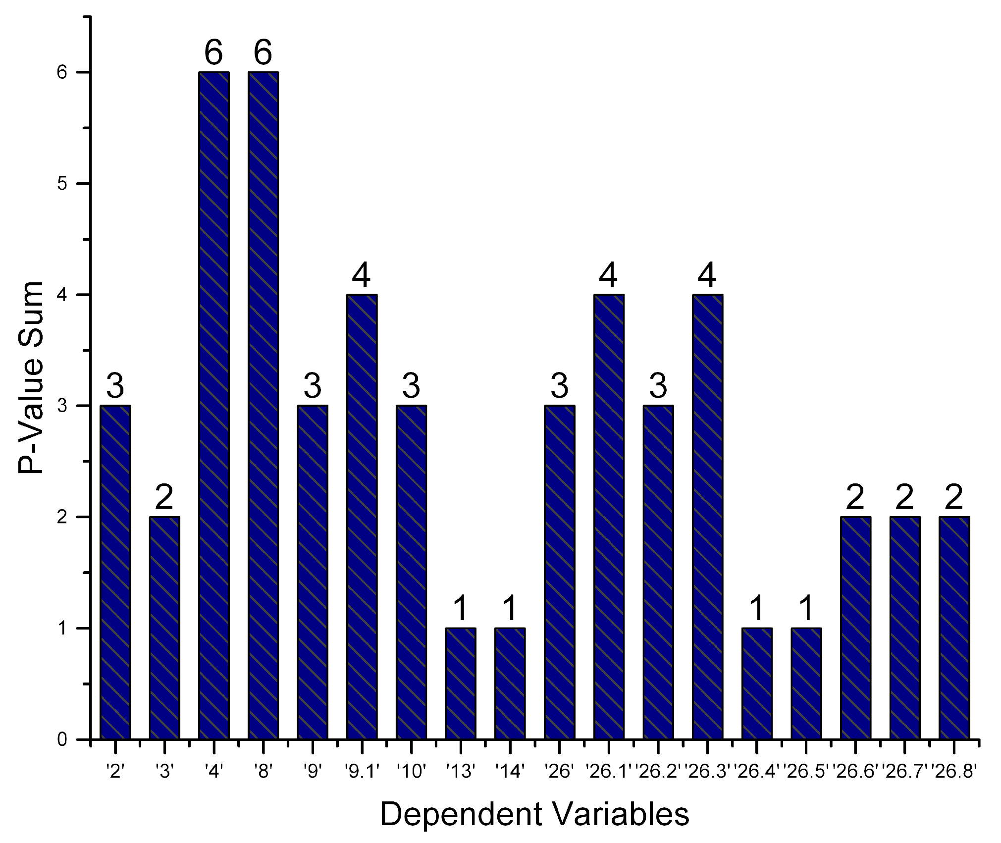
Figure 6, OLS regression is run for every regressand of the
x-axis. The corresponding number of regressors is depicted on the
y-axis, containing a value less than the threshold of 0.05 for the specific dataset. During the operation of a production line in real time, there is a constant flow of incoming recorded variables from the personnel. Therefore, the dynamic nature of the algorithm re-executes OLS regression at predefined time intervals to recreate the depiction of the Figure. Next, re-evaluation takes place for the impact the regressors inflict on the output sensor values. Regressands correlated to 6 regressors have a higher impact than those with a value of 1.
In
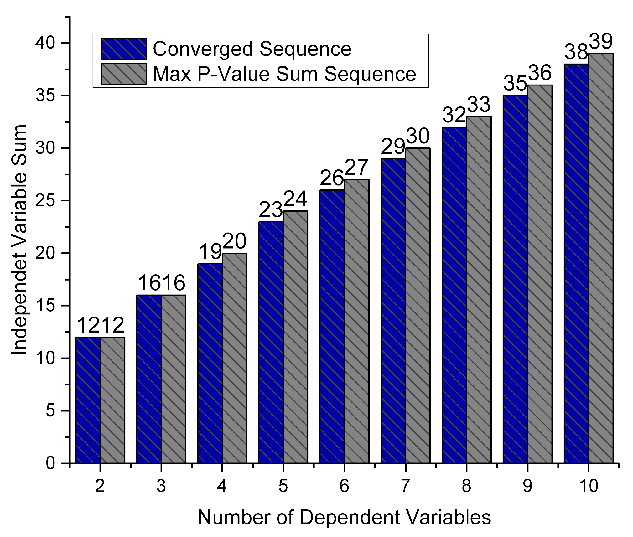
Figure 7, the
x-axis is the size of the regressand sequence. For each size, the converged sequence is found (carrying the highest
p-value sum that can be found heuristically using the LA system). Additionally, for the same sequence, the possible maximum sum is depicted. This way, the difference of the heuristic solution in contrast to the optimal solution is depicted. Since this difference is small (between 0–4%), the Orion heuristic algorithm, which is based on LA, is considered efficient for practical real-time execution.
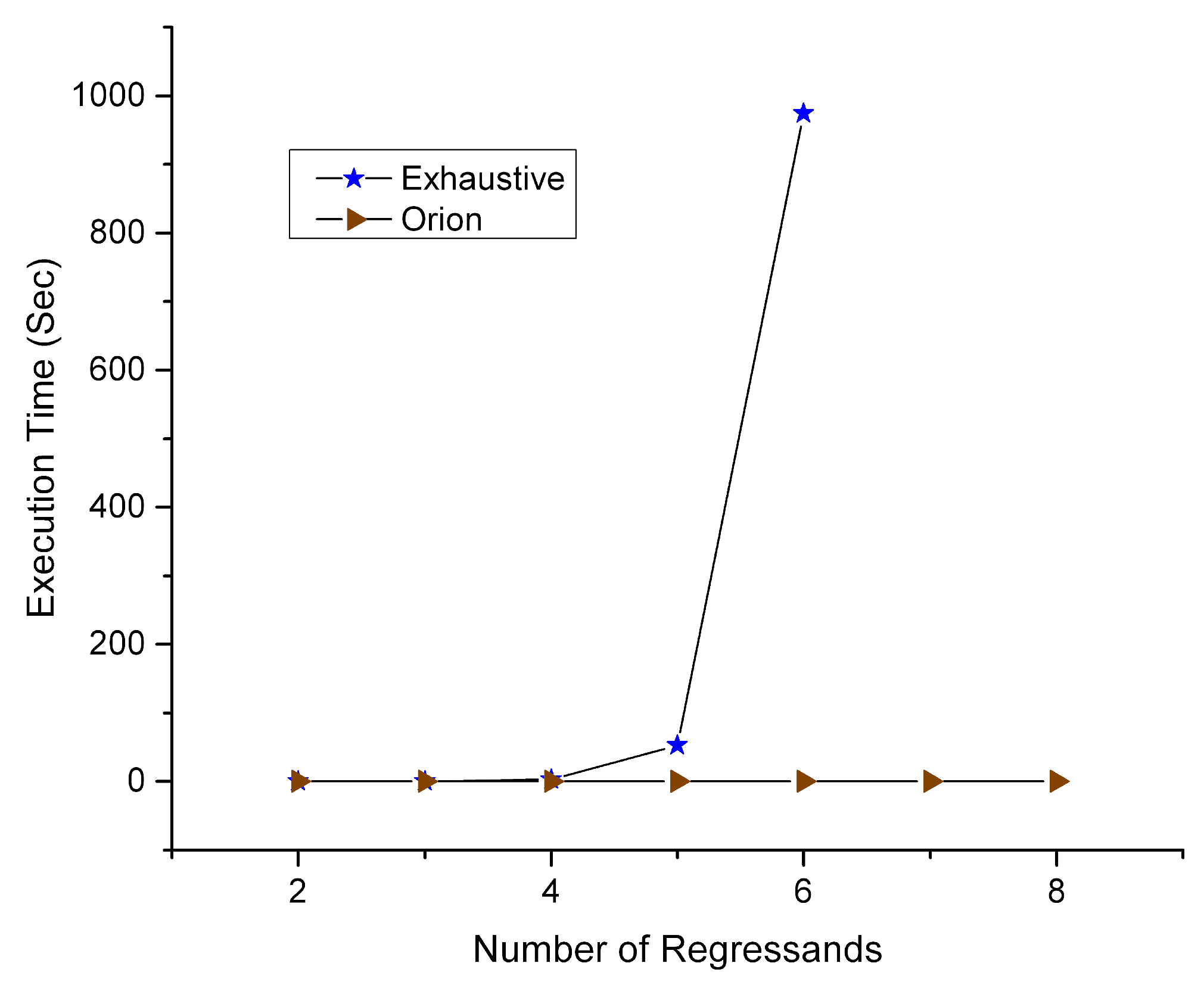
The execution time of Orion allows the algorithm to be realistically deployed. Specifically, when trying to execute a brute-force method to fetch the sequence of regressand values with the highest impact on regressors, limitations occur due to the high complexity. In
Figure 8, the execution time is depicted according to the increasing number of regressands. Practical results can only be obtained until their number reaches 6. Then, the complexity barrier causes the process to not provide results in a feasible time window. In contrast, Orion adapts to the runtime conditions and provides predictable behavior when the regressand number increases. The execution time is low and almost linear for the heuristic, and at the same time, it increases abruptly for the brute-force method, i.e., extends 1000 s for 6 variables. It cannot be calculated with a higher number of variables.
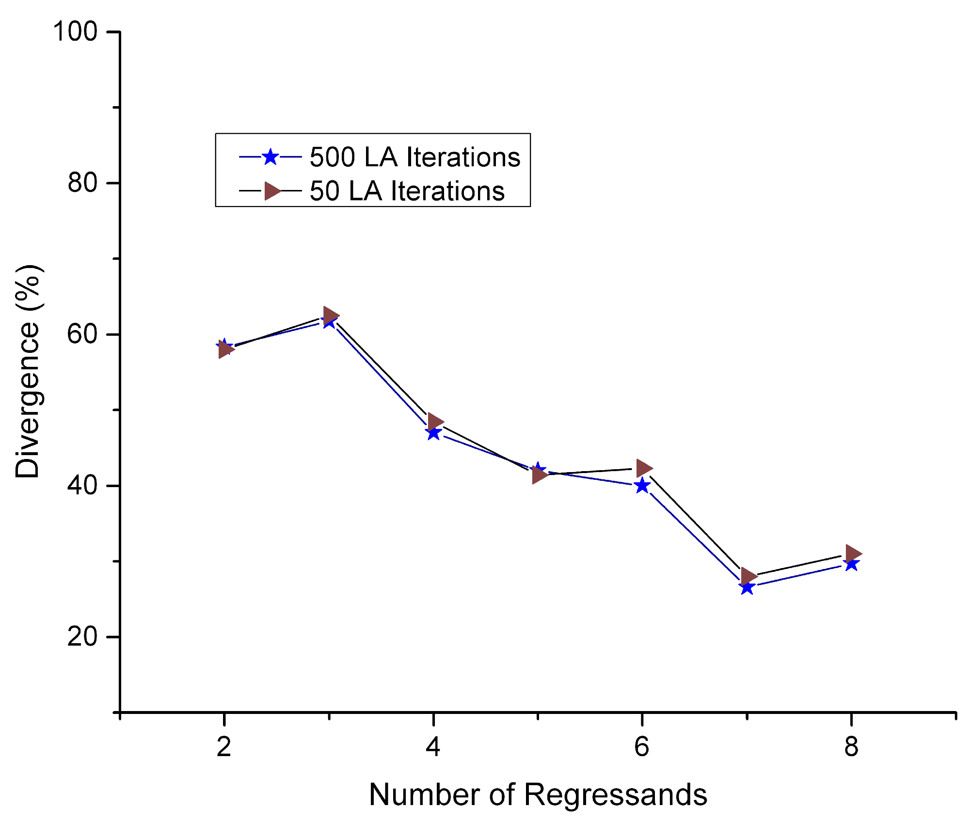
In
Figure 9, the percentage of divergence is depicted between the
p-value sum of a random sequence of regressand values and the sequence that is returned from the Orion algorithm. The former is chosen by a uniform distribution from all available dependent variables. As the number of regressands increases (
x-axis), the percentage of divergence decreases. When the number of variables is short, it is more possible for a uniform distribution to obtain distant values (in percentages) from the average. In the depicted value range of regressands, the divergence window is between 60% and 40%.


 ,
, 


