Article

Enhancing Positional Accuracy of the XY-Linear Stage Using Laser Tracker Feedback and IT2FLS

1
Faculty of Engineering, University of Nottingham, Nottingham NG7 2RD, UK
2
Department of Mechanical Engineering, Santa Clara University, Santa Clara, CA 95053, USA
*
Author to whom correspondence should be addressed.
Machines 2023, 11(4), 497; https://doi.org/10.3390/machines11040497
Submission received: 23 February 2023 / Revised: 13 April 2023 / Accepted: 14 April 2023 / Published: 20 April 2023
(This article belongs to the Special Issue Design and Control of Industrial Robots)

Abstract

:
This paper proposes a calibration algorithm to improve the positional accuracies of an industrial XY-linear stage. Precision positioning of these linear stages is required to maintain highly accurate object handling and manipulation. However, due to imprecisions in linear motor stages and the gearbox, static and dynamic errors exist within these manipulators that cannot be adjusted internally. In this paper, to improve the positioning accuracy of these manipulators, measurements from a laser tracker are used within an interval type-2 fuzzy logic system. The laser tracker used in this experiment is an AT960-MR, which is a highly accurate noncontact coordinate metrology equipment capable of performing highly accurate robotic measurements. To perform calibration, we use an IT2FLS to find a nonlinear correcting relationship to compensate for position errors. The IT2FLS acts on the commands given to the move stage to find the accurate position of the move stage. To train the IT2FLS, we use particle swarm optimization (PSO) for the antecedent part parameters and Moore–Penrose generalized inverse to estimate the consequent part parameters. Data are split into train/test data to test the efficacy of the proposed algorithm. It is shown that by using the proposed IT2FLS-based calibration approach, the standard deviation of the position errors can be decreased from 86.1μm to 55.9μm, which is a 35.1% improvement. Comparison results with a multilayer perceptron neural network reveal that the proposed IT2FLS-based calibration algorithm outperforms multilayer perceptron neural network for positional calibration purposes.

1. Introduction

Miniaturized and modularized linear move stage technology can be used within a highly precise manufacturing environment for efficient and high-precision object manipulation and object handling with micrometer and nanometer accuracy [1]. Linear stages have already been used within a wide range of applications, including single-axis nano-positioning [2], profiling stages [3], commercial atomic force microscopes [4], moving microscope probes [5], and micro-scale coordinate measurement machines [6].
The rotational motion of stepper motors is converted to linear motion using precision lead screw converters that are inevitably subject to manufacturing-related limitations and tolerances such as imperfect step sizes and dimensions, which leads to imprecise positioning. It is therefore required to calibrate linear stages to compensate for their positioning errors. The main sources of uncertainty within a linear move stage include angular uncertainties associated with its stepper motor, uncertainties regarding the lead screw converter, and uncertainties caused by the limited resolution of the shaft encoder. Moreover, for stacked XY-linear stages, the non-orthogonality between the X-linear stage and the Y-linear stage may impose more uncertainties for the overall linear move stage.
Previous approaches to calibrate move stages have been conducted using linear correcting equations and least squares approaches. A self-calibration technique has been investigated in [2] for a dual-actuated single-axis manipulator. The position feedback required for the calibration is provided using a simple artifact. The simplicity of this calibration approach makes it possible to conduct the calibration at the beginning of all automated processes. The capacitive sensors are considered to perform position measurements that are used for calibrations [2]. Having all measurements, a least squares algorithm is used to estimate the parameters of linear calibration equation. Scanning probe microscopes usually use linear stages in their structure. A self-calibration method to compensate for the non-orthogonality between the XY-plane and the Z-axis for scanning probe microscopes is investigated using some physical artifacts [5]. In this paper, an IT2FLS is used to compensate for the positional errors of linear move stages. Because of the capability of IT2FLSs to deal with nonlinear complex problems, they are the preferred choices in the current research to compensate for the nonlinear error of each individual stage and the error caused by non-orthogonality between the two move stages.
Because of the high precision of laser tracker systems, they are used to measure the true linear stage positions in this research to perform calibration. The first laser tracker system was invented in the 1980s to perform critical and highly accurate position measurements [7]. To date, this system is used to perform dimension measurements on large-scale aircraft workpieces [8,9], astronomical telescopes [10,11,12], position measurements for robotic systems [13,14,15], etc. [16]. The high precision and ease of application of the laser trackers make them a priority choice for the calibration of industrial robots and linear multi-axis linear stages. The precision position measurements required in this paper are performed using a high-precision laser tracker system.
In this paper, a novel calibration algorithm for XY-linear move stages is introduced. The proposed method uses the measurements from a highly precise laser tracker system, namely AT960-MR, to perform calibration. This equipment is a non-contact metrology tool capable of performing measurements with the error of less than 3 µm/m. Interval type-2 fuzzy systems (IT2FLSs) are strong general function approximations that are used to compensate for measurement errors. Since measurements are performed in two dimensions, the problem is solved using two IT2FLSs that share their antecedent part [17]. The implementation results show that using the proposed algorithm, it is possible to reduce the open-loop standard deviation of error in both X and Y dimensions from 86.1 μm to 55.9 μm, which is a 35.1% improvement. A multilayer perceptron neural network (MLPNN) is used to perform comparison. Comparison results reveal that IT2FLS is capable of performing calibration with higher performance.
This paper is organized as follows: The structure of interval type-2 fuzzy systems is explained in Section 2, and the experimental setup is presented in Section 3. In Section 4, the methodology part of the paper is presented. Experimental results are presented in Section 5. Concluding remarks and future works are presented in Section 6. The acknowledgments and the references are provided in backmatter, respectively.

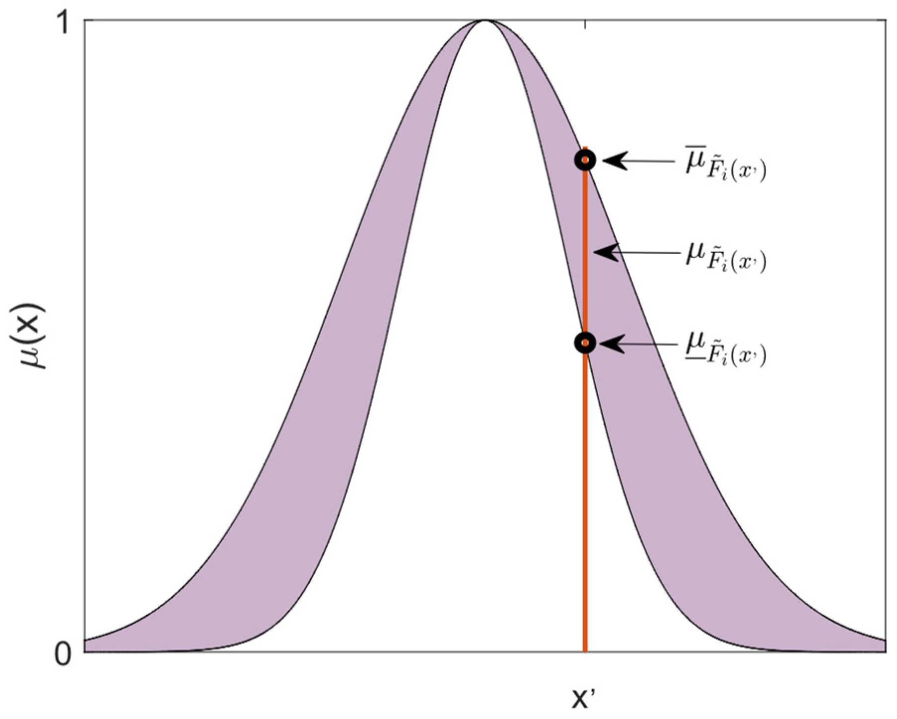
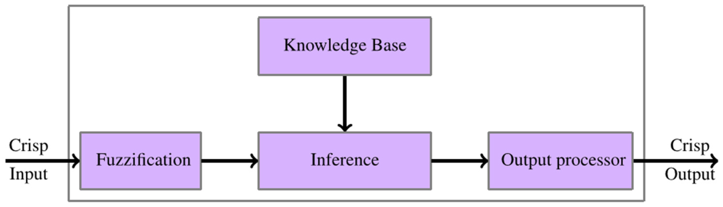
2. Interval Type-2 Fuzzy Systems Structure

In this paper, interval type-2 fuzzy MFs are used in the antecedent part, and interval values are considered for the consequent part parameters. The interval type-2 fuzzy MFs used in this paper are Gaussian MFs with certain center and interval values for the standard deviations (see Figure 1). The fuzzy IF-THEN rules for such a structure are considered as follows:
j - th   r u l e :   I F   x 1   i s   A ˜ j 1   a n d   x 2   i s   A ˜ j 2   T H E N   y j = α 1 j x 1 + α 2 j x 2 + β j ,   j = 1 , , M ,
where x 1 , and x 2 are the input variables, y is the single output variable, and M is the total number of the rules. Moreover, A ˜ j i s (I = 1, 2) are interval type-2 fuzzy MFs for the j-th rule of the i-th input. The parameters α i j and β j   i = 1 ,   2 ,   j = 1 , , M are the interval parameters in the consequent part of the rules that satisfy the following equation. The following definitions are made:
F j = α 1 j x 1 + α 2 j x 2 + β j ,   j = 1 , , M ,
w _ j x = μ _ F ˜ 1 j x 1 μ _ F ˜ 2 j x 2 ,   ( j = 1 , , M ) ,
w ¯ j x = μ ¯ F ˜ 1 j x 1 μ ¯ F ˜ 2 j x 2 ,   j = 1 , , M ,
where μ _ F ˜ k j x k , k = 1 ,   2 are μ ¯ F ˜ k j x k , k = 1 ,   2 are the lower and upper MF corresponding to the j -th rule for x k and “ ” is a t-norm operator. The output value of the IT2FLS, with its structure being as shown in Figure 2, is given as
Y x = y l x , y r x = w 1 w _ 1 , w ¯ 1 w M w _ M , w ¯ M 1 j = 1 M w j y j j = 1 M w j
where x = x 1 ,   x 2 R 2 is the IT2FLS input vector, representing the position readings from the move stage. The defuzzification process and the type-reduction are performed in an output processing unit (see Figure 2). There are several defuzzification + type-reduction methods for IT2FLSs [18,19,20]. The enhanced Karnik–Mendel model approach [21,22,23] is an exact yet computationally expensive type of defuzzifier + type reducer. A Maclaurin-based first-order approximator for an IT2FLS performs an approximation to the enhanced Karnik–Mendel (EKM) [21]. The accuracy of this method is lower than the enhanced Karnik–Mendel and higher than other approximate models of Biglarbegian–Melek–Mendel [24] and Nie–Tan [25,26]. The computational complexity for the Maclaurin-based first-order approximator is less than the EKM model, as it does not necessitate the sorting procedure required by EKM [27,28]. The Maclaurin-series-expansion-based first-order approximate output of the IT2FLS is as follows [27,28]:
y y l ,   y r ,
where y l and y r are the left-most and right-most values of output of the IT2FLS, which are calculated as follows:
y r j = 1 M ( w ¯ j + w _ j ) F j + j = 1 M s i g n m ¯ j Δ w j F j j = 1 M ( w ¯ j + w _ j ) + j = 1 M s i g n m ¯ j Δ w j
where
m ¯ j = F j j = 1 M w ¯ j F j j = 1 M w ¯ j
and Δ w j = w ¯ j w _ j . Furthermore, y l is calculated as
y l j = 1 M w ¯ j + w _ j F j j = 1 M s i g n m _ j Δ w j F j j = 1 M w ¯ j + w _ j j = 1 M s i g n m _ j Δ w j
where
m _ j = F j j = 1 M w _ j F j j = 1 M w _ j
The final crisp output value of the IT2FLS is obtained as
Y x = y l + y r 2 ,
It is then possible to rewrite (6) as
y r = j = 1 M ν R j F R j
where
ν R j = w ¯ j + w _ j + s i g n m ¯ j Δ w j j = 1 M w ¯ j + w _ j + j = 1 M s i g n m ¯ j Δ w j
The parameter y r in a vector form is obtained as:
y r = ϕ R θ ,
where
ϕ R = [ ν R T , ν R T x 1 , ν R T x 2 ] T ,
and α R is defined as
ν R = [ ν R 1 ,   ,   ν R M ] T .  
Furthermore, θ ¯ is defined as
θ n + 1 · M T = β 1 ,   ,   β M , α 11 , , α 1 M , α 21 , , α 2 M .
Similarly, it is possible to rewire the equation corresponding to y l in (8) in a vector form as
y l = j = 1 M ν l j F l j
where
ν l j = w ¯ j + w _ j s i g n m _ j Δ w j j = 1 M w ¯ j + w _ j j = 1 M s i g n m _ j Δ w j
The parameter y l in a vector form is obtained as
y l = ϕ L θ ,
where
ϕ L = [ ν L T , ν L T x 1 , ν L T x 2 ] T ,
and α L is defined as
ν L = [ ν L 1 ,   ,   ν L M ] T .
The pseudocode to find the output of IT2FLS is as follows.
  • Find the interval type-2 fuzzy membership functions μ _ F ˜ k j x k , k = 1 ,   2 are μ ¯ F ˜ k j x k , k = 1 ,   2 as follows
    μ _ F ˜ k j x k = e x p x k m k σ _ k 2 , k = 1 ,   2 μ ¯ F ˜ k j x k = e x p x k m k σ ¯ k 2 , k = 1 ,   2
  • Calculate w ¯ j and w _ j , j = 1, …, M as follows
    w ¯ j = μ ¯ F ˜ 1 j x 1 μ ¯ F ˜ 2 j x 2 ,   j = 1 , , M w _ j = μ _ F ˜ 1 j x 1 μ _ F ˜ 2 j x 2 ,   j = 1 , , M
  • Calculate m ¯ j , and m _ j as in (7) and (9), where F j is as defined as in (2).
  • Calculate y r , and y l as in (6) and (8).
  • Calculate y as in (10).
Figure 1. An interval type-2 fuzzy membership function.
Machines 11 00497 g001
Figure 2. An interval type-2 fuzzy system.
Machines 11 00497 g002

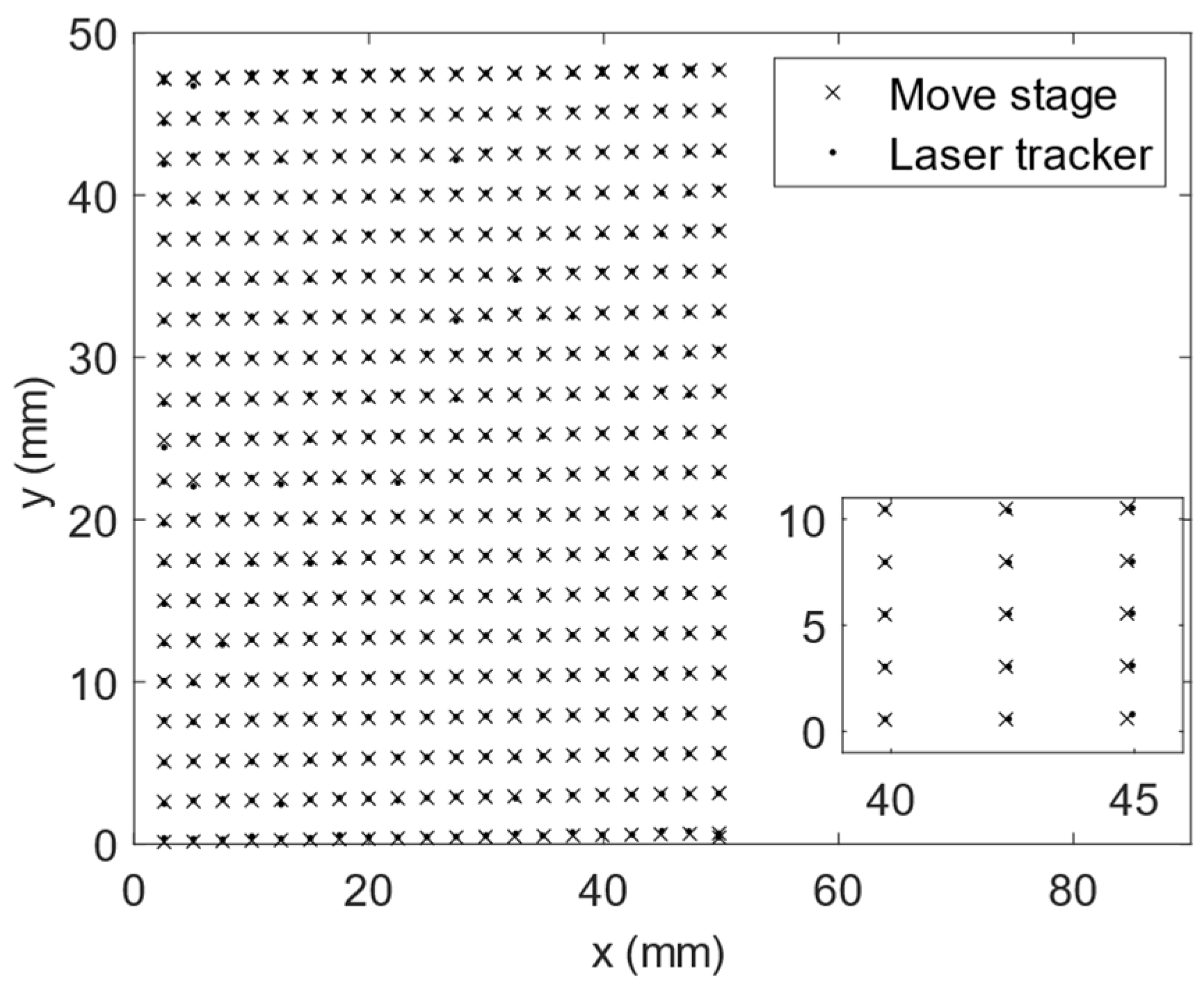
3. Experimental Setup
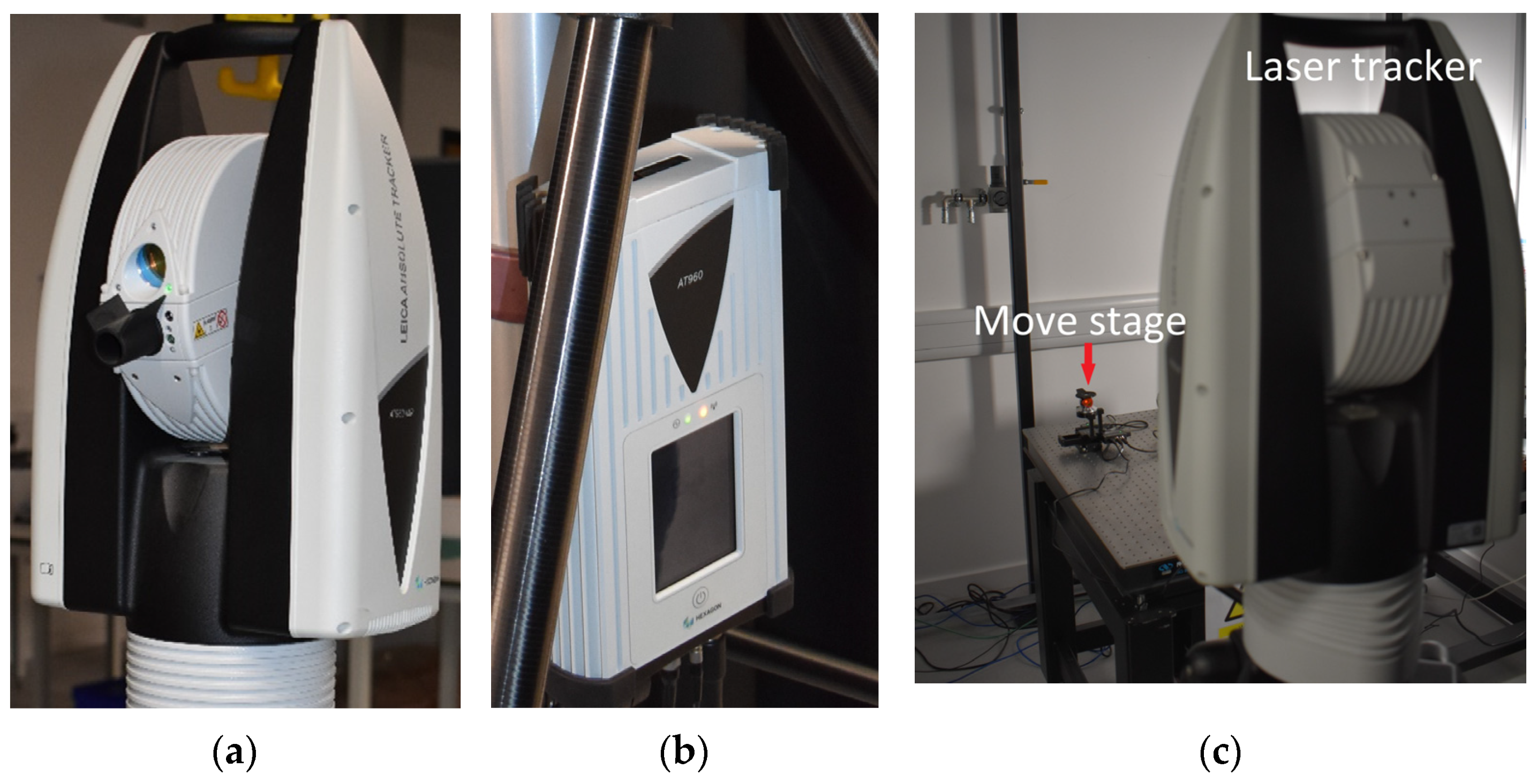
The experimental setup consists of an XY-linear move stage and a Leica laser tracker. The XY-linear stage is composed of two linear stages, which are mounted perpendicularly on each other. The feedback data provided by the Leica laser tracker is used to calibrate the position readings of the XY-linear stage. The detailed experimental setup is presented in this section.

3.1. Hardware Setup

To calibrate a linear move stage, a laser tracker system is set up at an approximately 2.8 m distance from the XY-linear stage. The technical specifications of the XY-linear stage and the laser tracker used in this paper are presented in this section.

3.1.1. Laser Tracker

The laser tracker system used for the calibration in this experiment is a Leica laser tracker AT960-MR manufactured by Hexagon Metrology GmbH, Wetzlar. It is a widely used measurement equipment in industries for precision distance measurements and position measurements [29] (see Figure 3). This equipment measures the distance between the laser tracker and the laser target mounted on a 3D-printed component on the XY-linear stage. The laser tracker target is a precision Leica 1.5” red ring reflector. The data is transferred via a Wi-Fi network connectivity between the laser tracker and a PC running Windows 10 OS. The software used to collect data is Spatial Analyzer® (SA) software. The operational frequency of the laser tracker is 10 Hz, and it can perform measurements up to 40 m, with errors less than 3   μ m / m . More details about the technical specifications of the laser tracker can be found in Table 1.

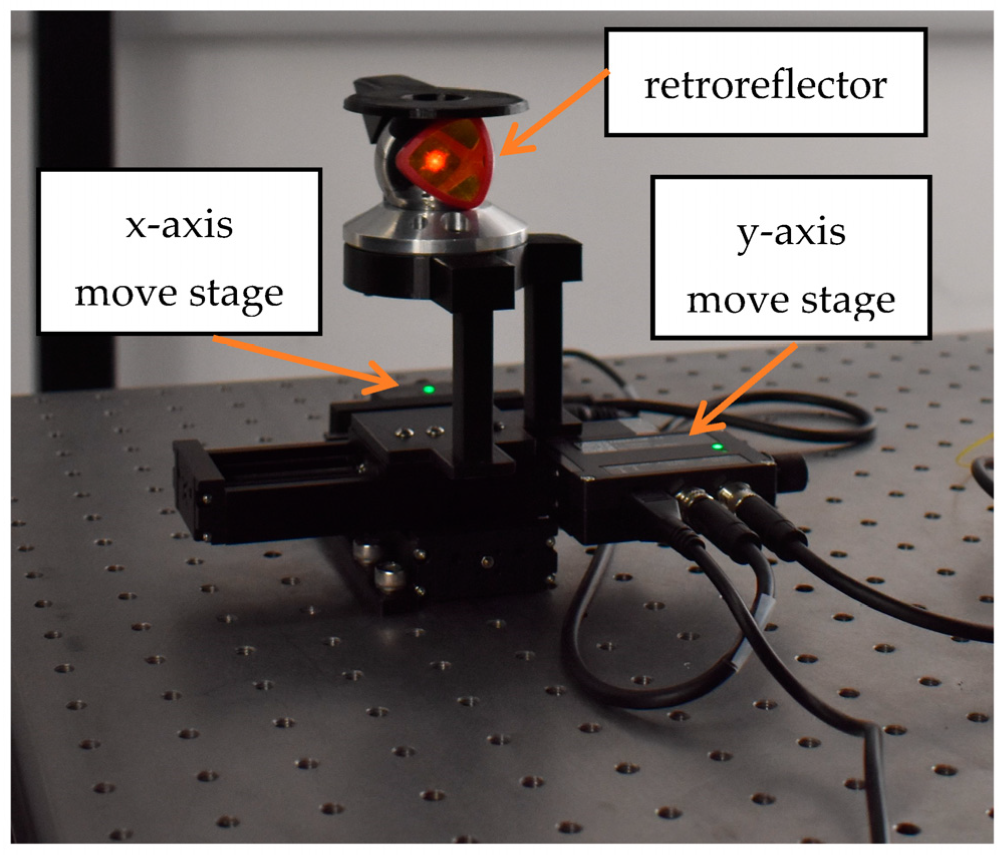
3.1.2. XY-Linear Stage

XY-linear stages produced by Zaber® are highly reliable products intended for critical medical, marine [30], aviation, 3D printing [31,32], and military applications (see Figure 4). As it is illustrated in Figure 4, the assembled XY-linear stage includes two linear stages: X-axis move stage and Y-axis move stage, which are assembled perpendicularly. The position feedback is provided via the retroreflector mounted on the XY-linear stage as the target for the laser tracker. The power supply for this linear stage is 24–48 VDC, and its maximum load capacity is 250 N. Each stage benefits from a two-phase stepper motor with a motor current rate of 600 mA/phase, and a precision lead screw converts the rotational movement to a linear one. It also benefits from a rotary quadrature encoder, with its resolution being equal to 800 states/rev. The micro-step sizes for this linear stage are equal to 0.047625 µm, its best accuracy is 15 µm, and its best repeatability is 3 µm. Furthermore, the highest speed of the stage is 104 mm/s, its highest trust is 55 N, and it benefits from the maximum load capacity of 250 N. When the move stages are mounted on top of each other to perform movements in more than single dimension, the position accuracy and repeatability of the overall system may be worse than the values associated with a single stage. The main reason is the perpendicularity error between the two stages. The communication interface between the PC and each linear stage is provided by an RS232 connection and the communication protocol is Zaber ASCII or Zaber binary. The maximum permeable connection baud rate is 115,200 bps, and a RS232/USB converter is provided within the linear stage to provide its connectivity with the PC. To sense the home position for the linear stage, a magnetic hall sensor is used. This product is controllable from the PC by using either Zaber Console software or Zaber Launcher software. Zaber motion libraries are also available under Python 3, C#, C++, JavaScript, Java, and MATLAB (https://www.zaber.com/software (accessed on 20 February 2023)). The Zaber linear stage may also be controlled using Arduino with the software library through the Zaber website (https://www.zaber.com/software (accessed on 20 February 2023)).
The data connection and the power connection for the first device are provided separately, and for the next stages, a Daisy chain connection provides power as well as data to control in a network fashion.

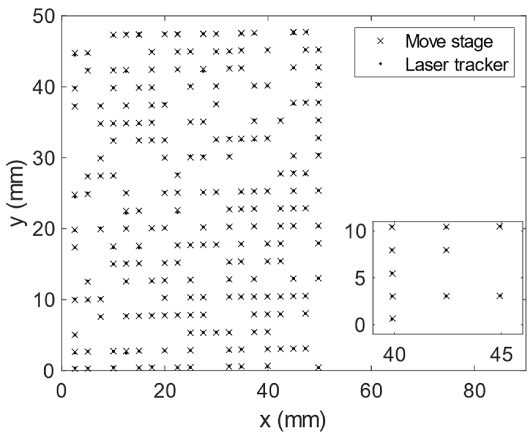
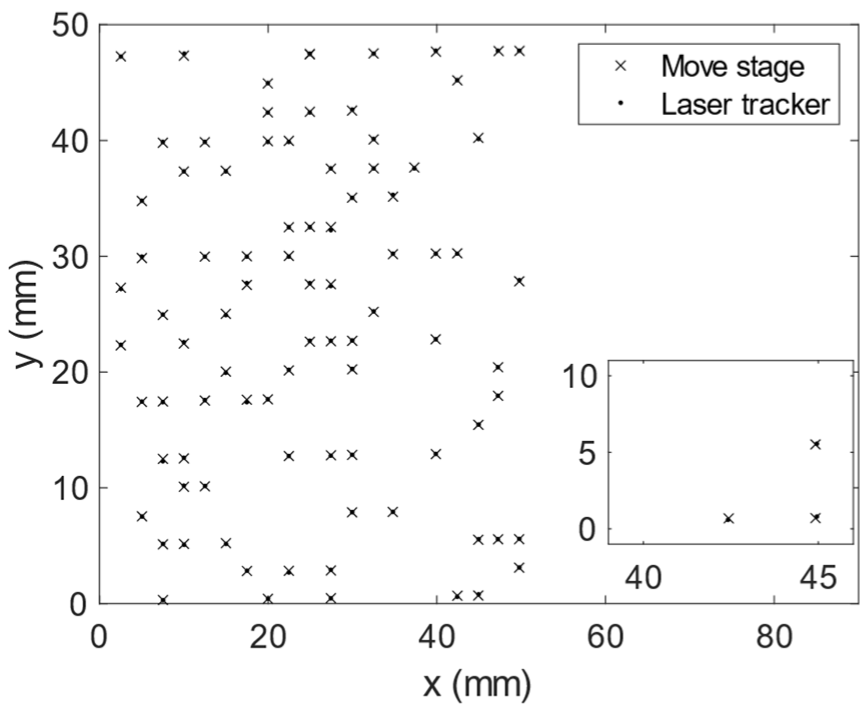
3.2. Data Resampling and Synchronization

In this paper, reference commands and the actual positions of the move stage are recorded using MATLAB® software (version R2021b) with Zaber Add-Ons. The laser tracker data are gathered using Spatial Analyzer software. As the start time and end time for data recording and the sample time for the move stage and the laser tracker are different, it is required to perform shift and resampling for the data gathered from the laser tracker and the move stage to ensure the data are properly synchronized.

3.3. Change in Coordinates

It is required to change the coordinate system to have the move stage positions available in the laser tracker coordinates. This is mainly required for the performance evaluation of the proposed IT2FLS based calibration algorithm.
x 1 r l x 2 r l = T r r l x 1 r r x 2 r r 1 ,
where x 1 r r , and x 2 r r are the move stage position readings obtained through its MATLAB® interface and x 1 r l , and x 2 r l are the move stage position readings using laser tracker in laser tracker coordinates, and T r r l R 2 × 3 is the transformation matrix from the robot base coordinate system to the coordinate system of the laser tracker. The transformation matrix T r r l can be easily calculated using a least squares algorithm [33].

4. Methodology

4.1. Particle Swarm Optimization

Metaheuristic approaches have been successfully applied to a wide range of applications where the cost function is not explicitly given and/or it suffers from multiple local minima. In this paper, inspired by previous applications of PSO in estimating the parameters of IT2FLSs, a PSO algorithm is used to estimate the IT2FLS parameters.
PSO is a variant of swarm intelligence primarily inspired by research on the behavior of swarms of birds and schools of fish [34]. The candidate solutions to this optimization problem are presented as a position vector corresponding to each individual within the swarm. The changes in the positions are determined by the velocity vector within each iteration. The velocity vector is updated by using a random term, preserving the previous velocity direction, and two other vectors, which guide particles towards the personal best experience of each particle and the overall global best experience. The individual solutions within the swarm are presented by X P S O i R d , where X P S O i refers to the i-th particle within the swarm, and d is the dimension of the solution space.
The positions in the next generation of PSO using its current position vector and velocity vector are updated as follows [34,35,36]:
V P S O i t + 1 = w V P S O i t + r 1 c 1 ( p b e s t i t X P S O i t ) + r 2 c 2 ( g b e s t i t X P S O i t ) ,   i = 1 , , N P ,
X P S O i t + 1 = X P S O i t + V P S O i t ,
where t refers to the current iteration, p b e s t i t presents the personal best experience of i-th particle, g b e s t i t represent the overall best experience within the swarm, 0 < c 1 ,   c 2 are the two positive constants, and r 1 ,     r 2 are two uniform random numbers from the interval of 0 ,   1 . The parameter c 1 is the coefficient associated with the best personal experiment of the particles in the swarm, and the parameter c 2 is the coefficient associated with the best global experiment of the particles within the swarm. The parameter w is the inertia weight, which makes the swarm follow their previous search direction. The parameter N P represents the total number of swarms. The stability criteria for PSO requires the following condition to be valid for its parameters [36,37].
c 1 + c 2 < 4 1 2 w + w 2 1 + w .
It is further observed in [38] that while large value for w improves exploration, a small value guarantees good exploitation capability for PSO.

4.2. Training IT2FLS

To train consequent part parameters of the IT2FLS, input/output training samples for it are considered as x i R n , y i R , i = 1 , , N , where N is the total number of samples.
y k = y r , k + y l , k 2 , k = 1 , , N , = 1 2 ϕ L , k θ + 1 2 ϕ R , k θ .
The overall input/output relationship in vectoral form is represented as follows.
Y = 0.5 Φ L θ + 0.5 Φ R θ ,
where Φ R   R N × 3 M , Φ L R N × 3 M , and Y R N × 1 are defined as follows.
Φ R = ϕ R , 1 T ϕ R , 2 T ϕ R , N T T ,
Φ L = ϕ L , 1 T ϕ L , 2 T ϕ L , N T T .  
Furthermore,
Y = Φ θ ,
where Φ , and θ are defined as follows:
Φ = Φ L T Φ R T T ,
The pseudo-inverse operator is used to find the solution for the estimation problem of the consequent part parameters as follows.
θ = Φ Y ,
where Φ is the Moore–Penrose generalized inverse of matrix Φ [39]. This concludes the consequent part parameters estimation problem.

4.3. Overall Hybrid Training Algorithm for IT2FLS

While the antecedent part parameters of IT2FLS appear nonlinearly within its output, its consequent part parameters appear linearly within the output. Hence, the least squares algorithm discussed in the previous subsection will be used for the consequent part parameters, and PSO is used to train the antecedent part parameters.
Figure 5 illustrates the overall flowchart of the proposed algorithm for training IT2FLSs for calibration purposes. The solutions in terms of the centers and the standard deviations of the antecedent part of the IT2FLS are represented by each individual member within PSO. The consequent part parameters of the IT2FLS need to be estimated according to (28)–(33). The inputs to the IT2FLS are the move stage command signals and their target values are the laser tracker data. The antecedent and consequent part parameters are evaluated against mean squared errors of their corresponding IT2FLS output. The personal best value of each individual member and the global best value of the overall swarm are updated accordingly. The PSO velocity update rule, as shown in (25) and (26), is then applied to each individual within the swarm to update the position of each individual. The algorithm iterates a few times before it is converged.

4.4. Overall Calibration Algorithm

The overall calibration algorithm consists of data gathering from the move stage using MATLAB and the laser tracker data using a Spatial Analyzer. Since data collected from the laser tracker and the move stage are gathered at different starting points and sampling frequencies, shift and resampling are required to have data from both devices synchronized (Section 3.2 and Section 3.3). The next stage requires applying the overall hybrid training algorithm to train IT2FLSs, as discussed in Section 4.3. To train the IT2FLS, we use PSO for the antecedent part parameters and Moore–Penrose generalized inverse to estimate the consequent part parameters. The overall flowchart of the proposed algorithm is demonstrated in Figure 5.

5. Experimental Results

The calibration methodology, explained in Section 4, is used to improve the positional accuracies in both X- and Y-directions, where position feedback is provided by the laser tracker system, Leica AT960-MR, used in these experiments. Figure 6 demonstrates the real-time position feedback by the laser tracker with the SA software. While Figure 6a shows the SA environment, Figure 6b demonstrates the zoomed-in version of Figure 6a in which the main axis as well as a few data points are demonstrated. It is required to set the axis and the coordinate origin of the laser tracker for measurements. To assign the coordinate origin as well as the X-axis and Y-axis, two initial large movements are performed using the XY-linear stage. The length of each movement is as high as 5 cm and is performed using each of the stages in the XY-linear stage. The axis assignment wizard menu of the Spatial Analyzer is used to define the two axes. The coordinate origin assignment as well as the axis assignment are required to be performed with high precision, as they influence all other 3D point measurements.
The uncertainties associated with positioning in a XY-linear stage are mainly due to stepper motor uncertainties, joint encoder uncertainties, and lead screw converter uncertainties. It is highly recommended to use calibration methods to improve the positional accuracies of XY-linear stages. The data gathered from the XY-linear stages are its command signal. The precise movement measurements are performed using the laser tracker. To perform the calibration task, the command signals given to the move stage are used as the input to an IT2FLS, and the target values for training IT2FLS are precise position measurements from the laser tracker. The input/output data are split to train and test data with a ratio of 70/30. The IT2FLS is tuned using the algorithm discussed in Section 4.3 and Section 4.4 (see Figure 5). The antecedent part of the IT2FLS is iterated using PSO, and the consequent part parameters are tuned using the Moore–Penrose generalized inverse. The Moore–Penrose generalized inverse of matrix Φ is implemented using the “pinv” built-in function in Matlab® software. The resulting IT2FLS gives the open-loop relationship between the commands given to the move stage and the real positions of the move stage. To provide precise XY-linear stage position feedback, a highly precise laser tracker system, Leica AT960-MR, is used. This laser tracker is capable of position measurements with errors of less than 3   μ m / m . The distance between the laser tracker and the target widely affects the measurement accuracy. The distance between the laser tracker system and its target is almost 2.8 m.
The initial data gathered from the move stage and the measurements performed using the laser tracker are provided in Figure 7. Least squares coordinate change is performed on the move stage positions to have all the positions in laser tracker coordinates. As can be seen from Figure 7, there exists some error in the move stage position commands with respect to the more precise position measurements performed by the laser tracker. The IT2FLS is then applied to the raw command signals given to the move stage for calibration purposes. The population size for the PSO is considered as equal to 1000, and in total, 200 iterations are used for the PSO. It is observed that using this approach, it is possible to decrease position errors in terms of the standard deviations of errors considerably.
Figure 8 and Figure 9 demonstrate the results of applying the calibration method to correct data within the X-axis and Y-axis, respectively. As can be seen from the figures, the calibrated position values are much closer to the measurements performed by the laser tracker. Table 2 illustrates the numerical values for the calibrated and uncalibrated position data. As can be seen from the table, the overall standard deviation of error has been reduced from 86.1 μm to 55.9 μm, which is a 35.1% improvement. To further analyze the proposed calibration scheme, the proposed algorithm is compared with a single layer MLPNN. The number of neurons taken for the hidden layer is selected equal to 10. As can be seen from the table, the IT2FLS outperforms MLPNN for the calibration of the move stage for both training and testing data in terms of standard deviation as well as mean absolute error.

6. Conclusions and Future Research

The uncertainties associated with an XY-linear stage are mainly due to stepper motor uncertainties, joint encoder uncertainties, and lead screw converter uncertainties. Tolerance in the manufacturing and assembly processes are the main causes of such uncertainties. The role of the lead screw converter is to convert the rotational movement of the motors to a linear movement. This part suffers from manufacturing tolerances and the uncertainties caused by wear and tear. The uncertainty caused by the non-orthogonal X-Y move stages is another source of uncertainty within an XY-linear stage. To calibrate the X-Y move stages, we used a high-precision laser tracker, namely Leica AT960-MR, which is capable of position measurements with errors of less than 3   μ m / m . Using the proposed algorithm, we showed that the standard deviation of positional errors associated with the XY-linear stage measurements decreased from 86.1 μm to 55.9 μm, which shows a 35.1% improvement. Furthermore, performance comparison of the proposed approach is provided with that of MLPNN. The result of the comparison reveals higher performance for the proposed approach over MLPNN calibration approaches.
As future work, closed-loop control methods to take advantage of the increased precision from this work with XY-linear stages will be investigated. The feedback from the laser tracker will be utilized to control the XY-linear stage online. The calibration results from the current experiment make it possible to decrease the rise time to track the reference trajectory for the XY-linear stage.

Author Contributions

Conceptualization M.A.K., M.Y., M.I., S.P., M.A.A. and D.T.B.; Data curation: M.A.K.; methodology, M.A.K.; software, M.A.K.; validation, M.A.K., formal analysis, M.A.K.; investigation, M.A.K.; resources, M.A.K.; writing—original draft preparation, M.A.K. and M.A.A. Writing—review and editing, M.A.K., M.Y., M.I., S.P., M.A.A. and D.T.B.; visualization, M.A.K. and M.A.A. supervision, S.P. and D.T.B.; project administration, S.P. and D.T.B.; funding acquisition, S.P. and D.T.B. All authors have read and agreed to the published version of the manuscript.

Funding

This work is primarily funded and supported by the Engineering and Physical Sciences Research Council (EPSRC) under grant number: EP/T023805/1—High-accuracy robotic system for precise object manipulation (HARISOM). The authors would also like to thank the UKRI Research England Development (RED) Fund for partial funding this work via the Midlands Centre for Data-Driven Metrology. The APC for this article is fully waived.

Data Availability Statement

Data would be available upon request on a personal contact with the corresponding author at the email address: mojtaba.ahmadiehkhanesar@nottingham.ac.uk.

Conflicts of Interest

The authors declare no conflict of interest.

References

  1. Yang, P.; Takamura, T.; Takahashi, S.; Takamasu, K.; Sato, O.; Osawa, S.; Takatsuji, T. Development of high-precision micro-coordinate measuring machine: Multi-probe measurement system for measuring yaw and straightness motion error of XY linear stage. Precis. Eng. 2011, 35, 424–430. [Google Scholar] [CrossRef]
  2. Jeong, Y.; Dong, J.; Ferreira, P. Self-calibration of dual-actuated single-axis nanopositioners. Meas. Sci. Technol. 2008, 19, 045203. [Google Scholar] [CrossRef]
  3. Yoo, S.; Kim, S.-W. Self-calibration algorithm for testing out-of-plane errors of two-dimensional profiling stages. Int. J. Mach. Tools Manuf. 2004, 44, 767–774. [Google Scholar] [CrossRef]
  4. Korpelainen, V.; Lassila, A. Calibration of a commercial AFM: Traceability for a coordinate system. Meas. Sci. Technol. 2007, 18, 395. [Google Scholar] [CrossRef]
  5. Xu, M.; Dziomba, T.; Dai, G.; Koenders, L. Self-calibration of scanning probe microscope: Mapping the errors of the instrument. Meas. Sci. Technol. 2008, 19, 025105. [Google Scholar] [CrossRef]
  6. Dang, Q.; Yoo, S.; Kim, S.-W. Complete 3-D self-calibration of coordinate measuring machines. CIRP Ann. 2006, 55, 527–530. [Google Scholar] [CrossRef]
  7. Muralikrishnan, B.; Phillips, S.; Sawyer, D. Laser trackers for large-scale dimensional metrology: A review. Precis. Eng. 2016, 44, 13–28. [Google Scholar] [CrossRef]
  8. Mei, B.; Zhu, W. Accurate positioning of a drilling and riveting cell for aircraft assembly. Robot. Comput.-Integr. Manuf. 2021, 69, 102112. [Google Scholar] [CrossRef]
  9. Guo, F.; Wang, Z.; Kang, Y.; Li, X.; Chang, Z.; Wang, B. Positioning method and assembly precision for aircraft wing skin. Proc. Inst. Mech. Eng. Part B J. Eng. Manuf. 2018, 232, 317–327. [Google Scholar] [CrossRef]
  10. Gale, D.M. Experience of primary surface alignment for the LMT using a laser tracker in a non-metrology environment. In Proceedings of the Ground-Based and Airborne Telescopes IV, Amsterdam, The Netherlands, 1–6 July 2012; Volume 8444, pp. 1649–1664. [Google Scholar]
  11. Rakich, A.; Bugonovic, D. A laser-tracker-target fiducialized alignment telescope for astronomical telescope alignment. In Proceedings of the Ground-Based and Airborne Telescopes IX, Montreal, QC, Canada, 17–22 July 2022; Volume 12182, p. 1218202. [Google Scholar]
  12. Burge, J.H.; Su, P.; Zhao, C.; Zobrist, T. Use of a commercial laser tracker for optical alignment. In Proceedings of the Optical System Alignment and Tolerancing, San Diego, CA, USA, 26–27 August 2007; Volume 6676, pp. 132–143. [Google Scholar]
  13. Lou, Z.; Zhang, J.; Gao, R.; Xu, L.; Fan, K.-C.; Wang, X. A 3D Passive Laser Tracker for Accuracy Calibration of Robots. IEEE/ASME Trans. Mechatron. 2022, 27, 5803–5811. [Google Scholar] [CrossRef]
  14. Wang, Z.; Zhang, R.; Keogh, P. Real-time laser tracker compensation of robotic drilling and machining. J. Manuf. Mater. Process. 2020, 4, 79. [Google Scholar] [CrossRef]
  15. Nguyen, V.; Cvitanic, T.; Baxter, M.; Ahlin, K.; Johnson, J.; Freeman, P.; Balakirsky, S.; Brown, A.; Melkote, S. Precision robotic milling of fiberglass shims in aircraft wing assembly using laser tracker feedback. SAE Int. J. Aerosp. 2022, 15, 87–97. [Google Scholar] [CrossRef]
  16. Khanesar, M.A.; Piano, S.; Branson, D. Improving the Positional Accuracy of Industrial Robots by Forward Kinematic Calibration Using Laser Tracker System. In Proceedings of the 19th International Conference on Informatics in Control, Automation and Robotics, Lisbon, Portugal, 14–16 July 2022. [Google Scholar]
  17. Xu, S.; An, X.; Qiao, X.; Zhu, L.; Li, L. Multi-output least-squares support vector regression machines. Pattern Recognit. Lett. 2013, 34, 1078–1084. [Google Scholar] [CrossRef]
  18. Wu, D. An overview of alternative type-reduction approaches for reducing the computational cost of interval type-2 fuzzy logic controllers. In Proceedings of the 2012 IEEE International Conference on Fuzzy Systems, Brisbane, Australia, 10–15 June 2012; pp. 1–8. [Google Scholar]
  19. Chen, C.; Wu, D.; Garibaldi, J.M.; John, R.I.; Twycross, J.; Mendel, J.M. A comprehensive study of the efficiency of type-reduction algorithms. IEEE Trans. Fuzzy Syst. 2020, 29, 1556–1566. [Google Scholar] [CrossRef]
  20. Mendel, J.M. Interval type-2 fuzzy systems. In Uncertain Rule-Based Fuzzy Systems: Introduction and New Directions, 2nd ed.; Springer: Cham, Switzerland, 2017; pp. 449–527. [Google Scholar]
  21. Wu, D.; Mendel, J.M. Enhanced karnik–mendel algorithms. IEEE Trans. Fuzzy Syst. 2008, 17, 923–934. [Google Scholar]
  22. Wu, D.; Mendel, J.M. Enhanced Karnik-Mendel algorithms for Interval Type-2 fuzzy sets and systems. In Proceedings of the NAFIPS 2007—2007 Annual Meeting of the North American Fuzzy Information Processing Society, San Diego, CA, USA, 24–27 June 2007; pp. 184–189. [Google Scholar]
  23. Greenfield, S.; Chiclana, F. Accuracy and complexity evaluation of defuzzification strategies for the discretised interval type-2 fuzzy set. Int. J. Approx. Reason. 2013, 54, 1013–1033. [Google Scholar] [CrossRef]
  24. Biglarbegian, M.; Melek, W.; Mendel, J. On the robustness of type-1 and interval type-2 fuzzy logic systems in modeling. Inf. Sci. 2011, 181, 1325–1347. [Google Scholar] [CrossRef]
  25. Nie, M.; Tan, W.W. Towards an efficient type-reduction method for interval type-2 fuzzy logic systems. In Proceedings of the 2008 IEEE International Conference on Fuzzy Systems (IEEE World Congress on Computational Intelligence), Hong Kong, China, 1–6 June 2008; pp. 1425–1432. [Google Scholar]
  26. Li, J.; John, R.; Coupland, S.; Kendall, G. On Nie-Tan operator and type-reduction of interval type-2 fuzzy sets. IEEE Trans. Fuzzy Syst. 2017, 26, 1036–1039. [Google Scholar] [CrossRef]
  27. Khanesar, M.A.; Mendel, J.M. Maclaurin series expansion complexity-reduced center of sets type-reduction+ defuzzification for interval type-2 fuzzy systems. In Proceedings of the 2016 IEEE International Conference on Fuzzy Systems (FUZZ-IEEE), Vancouver, BC, Canada, 24–29 July 2016; pp. 1224–1231. [Google Scholar]
  28. Khanesar, M.; Branson, D.T. Prediction interval identification using interval type-2 fuzzy logic systems: Lake water level prediction using remote sensing data. IEEE Sens. J. 2021, 21, 13815–13827. [Google Scholar] [CrossRef]
  29. Kyle, S. Operational features of the Leica laser tracker. In Proceedings of the IEE Seminar on Business Improvement through Measurement, Birmingham, UK, 8 June 1999. [Google Scholar]
  30. Dusek, J.E.; Triantafyllou, M.S.; Lang, J.H. Piezoresistive foam sensor arrays for marine applications. Sens. Actuators A Phys. 2016, 248, 173–183. [Google Scholar] [CrossRef]
  31. Castellanos-Ramos, J.; Navas-González, R.; Fernández, I.; Vidal-Verdú, F. Insights into the mechanical behaviour of a layered flexible tactile sensor. Sensors 2015, 15, 25433–25462. [Google Scholar] [CrossRef]
  32. Arrington, C.B.; Rau, D.A.; Williams, C.B.; Long, T.E. UV-assisted direct ink write printing of fully aromatic Poly (amide imide) s: Elucidating the influence of an acrylic scaffold. Polymer 2021, 212, 123306. [Google Scholar] [CrossRef]
  33. Fotiou, A.; Kaltsikis, C. Computationally efficient methods and solutions with least squares similarity transformation models. Living GIS 2016, 2, 2018. [Google Scholar]
  34. Yang, X.-S.; Deb, S.; Zhao, Y.-X.; Fong, S.; He, X. Swarm intelligence: Past, present and future. Soft Comput. 2018, 22, 5923–5933. [Google Scholar] [CrossRef]
  35. Chakraborty, A.; Kar, A.K. Swarm intelligence: A review of algorithms. In Nature-Inspired Computing and Optimization: Theory and Applications; Springer: Cham, Switzerland, 2017; pp. 475–494. [Google Scholar]
  36. Dong, W.Y.; Zhang, R.R. Order-3 stability analysis of particle swarm optimization. Inf. Sci. 2019, 503, 508–520. [Google Scholar] [CrossRef]
  37. Kadirkamanathan, V.; Selvarajah, K.; Fleming, P.J. Stability analysis of the particle dynamics in particle swarm optimizer. IEEE Trans. Evol. Comput. 2006, 10, 245–255. [Google Scholar] [CrossRef]
  38. Wang, F.; Zhang, H.; Zhou, A. A particle swarm optimization algorithm for mixed-variable optimization problems. Swarm Evol. Comput. 2021, 60, 100808. [Google Scholar] [CrossRef]
  39. Hassan, S.; Khanesar, M.A.; Hussein, N.K.; Belhaouari, S.B.; Amjad, U.; Mashwani, W.K. Optimization of interval type-2 fuzzy logic system using grasshopper optimization algorithm. Comput. Mater. Contin. 2022, 71, 3513–3531. [Google Scholar] [CrossRef]
Figure 3. Laser tracker: (a) camera; (b) controller; (c) overall system.
Machines 11 00497 g003
Figure 4. XY-linear move stage.
Machines 11 00497 g004
Figure 5. Flowchar of the proposed training method for IT2FLS for calibration.
Machines 11 00497 g005
Figure 6. Spatial analyzer software environment (a) whole software screenshot; (b) zoomed in position data.
Machines 11 00497 g006
Figure 7. Move stage commands with coordinate change versus laser tracker measurements.
Machines 11 00497 g007
Figure 8. Calibration using IT2FLS for training data.
Machines 11 00497 g008
Figure 9. Calibration using IT2FLS for testing data.
Machines 11 00497 g009
Table 1. Measuring equipment characteristics and specifications.
Environmental Working ConditionsIP54: The IEC-Certified Sealed Unit Guarantees Ingress Protection against Dust and Other Contaminants
Operating temperatureWide operating temperature range of −15 to 45 degrees Celsius
Temperature compensationMeteoStation: Integrated environmental unit monitors conditions including temperature, pressure, and humidity to compensate for changes
ISO certificationISO 17025
ConnectivityWifi and LAN
Detector featuresRed ring reflector—1.5” radius: 19.05 mm ± 0.0025 mm, centring of optics: < ±0.003 mm, ball roundness: ≤0.003 mm, acceptance angle: ±30°, weight: 170 g
Data output rateMeasurement rate of up to 1000 points per second
Distance accuracy40 m in diameter and a 6DoF measuring volume of up to 20 m
Laser safetyLaser class 2
Table 2. XY-mean absolute error and standard deviations of error for the linear stage.
Performance Indexes Calibrated   Using   IT 2 FLS   ( μ m ) Calibrated   Using   MLPNN   ( μ m ) Uncalibrated   ( μ m ) Percentage Improvement of IT2FLS vs. Raw Data
MAETrain41.650.452.420.6%
σ i 68.868.379.113.0%
MAETest34.249.758.241.2%
σ i 55.969.886.135.1%
Disclaimer/Publisher’s Note: The statements, opinions and data contained in all publications are solely those of the individual author(s) and contributor(s) and not of MDPI and/or the editor(s). MDPI and/or the editor(s) disclaim responsibility for any injury to people or property resulting from any ideas, methods, instructions or products referred to in the content.

