Simulation and Validation of Cavitating Flow in a Torque Converter with Scale-Resolving Methods

Abstract

The purpose of this paper is to study the mechanism and improve the prediction accuracy of transient torque converter cavitation flow by the application of scale-resolving simulation (SRS) methods with particular focus on cavitation vortex flow. Firstly, the numerical analysis of the entire internal flow field of the torque converter was carried out using different turbulence models, and the prediction accuracy of the hydraulic characteristics of the adopted models was analyzed and validated via test data. Secondly, the cavitation and turbulence behavior in the internal flow field were analyzed, and the blade surface pressure according to different turbulence models was compared and validated through test data. Finally, the transient cavitation characteristics of the flow field were studied based on the stress-blended eddy simulation (SBES) model. The prediction accuracy of the cavitation flow field simulation of the torque converter is significantly improved using the SRS model. The maximum error of capacity constant, torque ratio and efficiency are reduced to 3.1%, 2.3%, and 1.3% at stall, respectively. The stator is more prone to cavitation than pump and turbine. The SBES model has the highest prediction accuracy in multiple measurement points, and the maximum deviation can reach 13.32% under stall. Attached cavitation bubbles and periodic shedding cavitation can be found in the stator, and the evolution period is about 0.0036 s, i.e., 279 Hz. The prediction accuracy of different models was compared and analyzed, which has important guiding significance for the high-precision prediction and analysis of fluid machinery.

1. Introduction

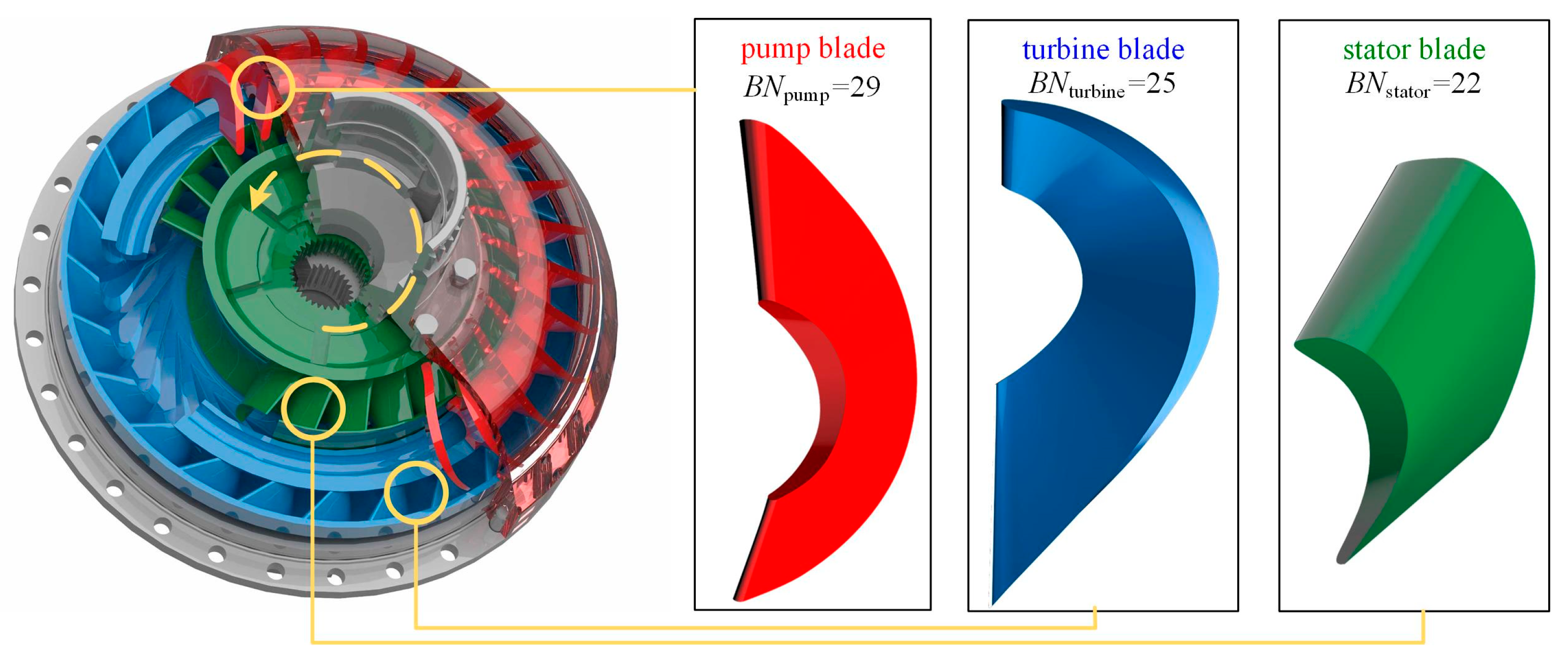
Torque converters are mainly composed of a pump, a turbine and a stator, as shown in Figure 1. Each impeller contains a cascade with different blade shapes, and the fluid circulates inside the torque converter to transmit power and energy [1]. The oil in the high-speed rotating pump flows at a higher speed under the action of centrifugal force, the high-speed oil enters the turbine and impacts the turbine blades, causing the turbine to rotate, after flowing out of the turbine into the stator to convert part of the kinetic energy into pressure potential energy and achieve flow guidance. With the increasing interest in heavy-load and high-power-density transmissions, the torque converter is also developing in the direction of higher capacity constant and smaller dimensions, resulting in higher fluid velocity, more complicated vortex flows and secondary flows in different degrees. The liquid flow velocity inside the torque converter can reach up to 30 m/s during severe operating conditions, leading to low local pressure and making the torque converter more prone to cavitation. The occurrence of cavitation has an important impact on the performance, reliability, and service life of the fluid machines. It can lead to violent impacts on the impeller and damage to the impeller surface material [2].

At present, most scholars are focusing on the cavitation characteristics of the torque converter flow field in various operating conditions. Liu Cheng et al. revealed the fluid field mechanism of the influence of charging oil conditions on torque converter cavitation behavior, providing practical guidelines for suppressing cavitation in torque converters [3]. Ran et al. developed a cavitation suppression technique by slotting one side of the stator suction side, which was proven to be able to significantly shorten the cavitation duration [4]. Guo et al. developed a full-flow passage geometry and a computational fluid dynamics (CFD) model with cavitation to analyze the flow behavior in the torque converter [5]. Xiong et al. optimized the Joukowsky airfoil used in the design of the stator blades, which greatly reduced the probability of cavitation and improved the performance and service life of the torque converter [6].

It was found in many studies that the complex turbulent structure often interacted with the occurrence of cavitation. Aliakbar et al. compared the vortex performance of two-dimensional NACA 0012 and NACA 6612 hydrofoils under different cavitation and non-cavitation conditions [7]. In order to predict and analyze the cavitation characteristics of the torque converter, it is very important to accurately capture the turbulent structure in both spatial and temporal dimensions. At present, most of the numerical calculations of fluid machinery are based on the RANS model. Yang et al. examined the impact of the viscosity and the density of transmission fluids on the performance of a hydraulic torque converter by the SST k-ω model [8]. Zheng et al. carried out multi-objective optimization design for the blade angles by incorporating three-dimensional steady computational fluid dynamics numerical simulation with the SST k-ω turbulence model [9]. Cheng et al. used a k-ε model to capture blade surface load data for a two-way interaction model [10]. The RANS model is more widely used in the parametric design of impellers due to its low consumption of computing resources [11,12,13,14,15].

Scale-resolving simulation (SRS) methods, as a divide-and-conquer strategy for resolution of the entire turbulent spectrum in the entire flow domain, have been widely applied in high-precision simulation of various flow fields. Florian provided an overview of scale-resolving simulation (SRS) methods used in ANSYS CFD software [16]. H.Y. Cheng et al. carried out numerical simulations of a tip leakage cavitation with the large eddy simulation (LES) method combined with the Schnerr–Sauer cavitation model with high-speed flow around a NACA 0009 hydrofoil [17]. The LES was applied for the flow field simulation of special-shaped channel-parts; sub-grid models were analyzed and compared [18]. Wang et al. applied the large eddy simulation approach to comprehensively reveal the unsteady cavitating flow features of a twist hydrofoil, and validated the findings against the experimental result [19].

Some scholars have also explored the use of hybrid RANS/LES (HRL) model for computational analysis of fluid machinery. Li et al. applied the volume-of-fluid (VOF) method and an SRS model to calculate and analyze the flow field in a retarder considering the cavitation phenomenon [20]. Liu et al. applied four typical SRS models to conduct numerical simulations of the internal flow fields for hydraulic components [21].

Many scholars have found an interactive relationship between eddy currents and cavitation in their studies. Xie et al. found that the cavitation promoted the production of vorticity and increased the boundary layer thickness [22]. Wu et al. investigated the cavitating flow in the wake of a wedge-shaped bluff body, and the role of the presence of high void-fraction regions in the near-wake region on the process of vortex formation and shedding [23]. It was found that by changing the wall surface roughness, the velocity component inside the blade tip vortex was reduced, the generation of tip vortex cavitation (TVC) was alleviated, and the cavitation volume fraction of the flow field was further reduced [24]. Some research results show that the interaction between vortices and turbulence exhibited a high degree of consistency in the wake flow [25].

Different CFD models were developed in ANSYS CFX^TM to predict the torque converter fluid behavior based on Reynolds-averaged Navier–Stokes equations. Considering that SRS takes advantage of LES to better resolve different scales of vortex as well as cavitation [26], the application of SRS simulation should be the trend for the analysis of complex cavitation phenomena. Herein, a series of SRS and RANS models were applied in the calculations of torque converter cavitation flow, and the results were validated through both overall hydrodynamic performance tests and internal pressure measurements. The study provided detailed insight into the mechanism of the interaction between turbulence and cavitation and practical guidance for the selection of turbulence models in terms of torque converter cavitation simulation.

2. Computational Model

2.1. Turbulence Model

Turbulence is a complex process mainly because it is three dimensional, unsteady and consists of many scales. It has a significant effect on the characteristics of the flow. Turbulence occurs when the inertia forces in the fluid become significant compared to viscous forces, and is characterized by a high Reynolds Number.

In principle, the Navier–Stokes equations describe both laminar and turbulent flows without the need for additional information. However, turbulent flows at realistic Reynolds numbers span a large range of turbulent length and time scales, and would generally involve length scales much smaller than the smallest finite volume mesh. The Direct Numerical Simulation (DNS) of these flows would require computing power that is many orders of magnitude higher than available in the foreseeable future.

In order to predict the effects of turbulence, a large amount of CFD research has concentrated on methods that make use of turbulence models. In this paper, several representative SRS models were selected to simulate the occurrence of cavitation in the torque converter flow field, which includes DDES, SBES and SAS-SST [27]. As a control group, the representative of the RANS turbulence model--SST model and LES subgrid model--WALE model, are also used in flow field simulations [28]. The advantages and disadvantages of above turbulent models are shown in

Table 1. Features of different turbulence models.

Model	Feature
SST (Shear Stress Transport model)	Based on the RANS ideology. Widely used in the flow field calculation of fluid machinery, with low grid fineness requirements and short calculation time, and the calculation error is large.
WALE (wall-adapting local eddy-viscosity model)	Belongs to the LES subgrid model. Has the capability to reproduce laminar to turbulent transition. The amount of calculation is too large, while accuracy of results depends on mesh size and quality.
DDES (Delayed Detached Eddy Simulation)	Belongs to the HRL algorithm. DDES combines the advantages of RANS and LES, requires lower boundary layer grids than LES, and has better computational robustness and accuracy
SBES (Stress-Blended Eddy Simulation)	Belongs to the HRL algorithm. SBES introduces a hybrid function, which can generically combine RANS and LES model formulations. It has a rapid “transition” from RANS to LES in separating shear layers.
SAS-SST (SAS based on SST model)	Belongs to the HRL algorithm. SAS is an improved URANS formulation, which allows the resolution of the turbulent spectrum in unstable flow conditions. It has better robustness and must perform fewer calculations than WALE.

.

2.1.1. SST Model

The SST model is based on the k-ω equation. The turbulent kinetic energy (k) equation and specific dissipation rate (ω) equation are expressed as follows [29,30]:

$$\frac{\partial }{\partial t}\left(\rho k\right)+\frac{\partial }{\partial x_j}\left(\rho k{u}_j\right)=\frac{\partial }{\partial x_j}\left[\left(\mu +{\sigma }_k{\mu }_t\right)\frac{\partial k}{\partial x_j}\right]+{\mu }_t\frac{\partial u_i}{\partial x_j}\left(\frac{\partial u_i}{\partial x_j}+\frac{\partial u_j}{\partial x_i}\right)-{\beta }^{*}\rho k\omega$$

(1)

$$\frac{\partial }{\partial t}\left(\rho \omega \right)+\frac{\partial }{\partial x_j}\left(\rho \omega u_j\right)=\frac{\partial }{\partial x_j}\left[\left(\mu +{\sigma }_{\omega }{\mu }_t\right)\frac{\partial \omega }{\partial x_j}\right]+\alpha \rho S^2-\beta \rho {\omega }^2+2\left(1-F_1\right)\frac{\rho {\sigma }_{\omega 2}}{\omega }\frac{\partial k}{\partial x_j}\frac{\partial \omega }{\partial x_j}$$

(2)

where μ is the dynamic viscosity, x_i and u_i represent a coordinate axis and the corresponding speed, respectively, S is the strain rate, and σ_k, σ_ω, σ_ω2, and β* are model parameters. The mixing function F₁ is define by

$$F_1=\tan \mathrm{h}{\left\{\min \left[\max \left(\frac{\sqrt{k}}{{\beta }^{*}\omega y},\frac{500\mu }{\rho y^2\omega }\right),\frac{4\rho {\sigma }_{\omega 2}k}{{\mathrm{CD}}_{k\omega }{y}^2}\right]\right\}}^4$$

(3)

$${\mathrm{CD}}_{k\omega }=\max \left(2\rho {\sigma }_{\omega 2}\frac{1}{\omega }\frac{\partial k}{\partial x_j}\frac{\partial \omega }{\partial x_j},{10}^{-10}\right)$$

(4)

The turbulent viscosity μ_t is defined as

$${\mu }_t=\frac{{\alpha }_{1}k}{\max \left({\alpha }_1\omega ,S{F}_2\right)}$$

(5)

where F₂ is also the mixing function, which is

$$F_2=\tan \mathrm{h}{\left[\max \left(\frac{2\sqrt{k}}{{\beta }^{*}\omega y},\frac{500\mu }{\rho y^2\omega }\right)\right]}^2$$

(6)

2.1.2. DDES Model

The DDES model is an improved DES model based on the HRL algorithm theory. Since the DES methods can be constructed through modification of the destruction term of the turbulent kinetic energy transport equation, the k-equation in DDES can be given by:

$$\frac{\partial \left(\rho k\right)}{\partial t}+\frac{\partial \left(\rho u_{j}k\right)}{\partial x_j}=P_k-D_k+\frac{\partial }{\partial x_j}\left[\left(\mu +{\sigma }_k{\mu }_t\right)\frac{\partial k}{\partial x_j}\right]$$

(7)

where ${\mu }_t$ denotes the turbulent viscosity. The production term and the destruction term are given by

$$\begin{array}{c}{P}_k={\tau }_{ij}\overline{S_{ij}}\\ D_k=\rho k^{3/2}/l_{\mathrm{DDES}}\end{array}$$

(8)

Differing from the DES-SST proposed by Strelets (2001), the hybrid length scale $l_{\mathrm{D}\mathrm{D}\mathrm{E}\mathrm{S}}$ for DDES can be defined as

$$l_{\mathrm{DDES}}=\min \left(l_{\mathrm{RANS}};\frac{l_{\mathrm{LES}}}{1-F_{\mathrm{SST}}}\right)$$

(9)

This length scale can switch between the turbulence length scale $l_{\mathrm{R}\mathrm{A}\mathrm{N}\mathrm{S}}$ and the filter length scale $l_{\mathrm{L}\mathrm{E}\mathrm{S}}$, which are defined as

$$\begin{array}{c}{l}_{\mathrm{RANS}}=\frac{k^{1/2}}{{\beta }^{*}\omega },l_{\mathrm{LES}}=C_{\mathrm{DES}}{\Delta }_{\mathrm{DDES}},\\ {\Delta }_{\mathrm{DDES}}=\max \left(\delta x,\delta y,\delta z\right),\end{array}$$

(10)

$${\Delta }_{\mathrm{DDES}}=\max \left(\delta x,\delta y,\delta z\right)$$

(11)

where Δ_DDES is related to the maximum local mesh spacing as the filter width and β^∗ denote constants of the original Wilcox model [31]. F_SST is a damping parameter taking the form in the SST model [32], which offers the highest level of protection against grid-induced separation.

2.1.3. SBES Model

The SBES model can be switched between the RANS and LES models. It reconfigures the hybrid functions to provide a more reasonable boundary layer protection mechanism to limit premature switching to the LES model. Premature switching reduces the ability of the RANS model to simulate the underlying boundaries. The SBES model adds a sink term ε_SBES to the equation, as shown in the following [29]:

$${\epsilon }_{\mathrm{SBES}}=-{\beta }^{*}\rho k\omega F_{\mathrm{SBES}}$$

(12)

$$F_{\mathrm{SBES}}=\max \left(\frac{l_{\mathrm{t}}}{C_{\mathrm{SBES}}{\Delta }_{\mathrm{SBES}}}\left(1-f_{\mathrm{s}}\right),1\right)-1,$$

(13)

where C_SBES is the model parameter, and Δ_SBES is the grid size. fs is used in the blending function to combine the stress term in the SST model and the LES model as follows:

$${\tau }_{ij}^{\mathrm{SBES}}=f_{\mathrm{s}}{\tau }_{ij}^{\mathrm{SST}}+\left(1-f_{\mathrm{s}}\right){\tau }_{ij}^{\mathrm{LES}}$$

(14)

where ${\tau }_{ij}^{\mathrm{SST}}$ and ${\tau }_{ij}^{\mathrm{LES}}$ are the modeling stress tensors for the SST and the LES models, respectively, and ${\tau }_{ij}^{\mathrm{SBES}}$ is the stress tensor for the SBES model.

2.1.4. SAS-SST Model

SAS-SST is an improved URANS formulation. This approach allows the representation of the large scales of turbulence [33,34]. The only difference between RANS and SAS formulations is the additional source term denoted Q_SAS in the transport equation for the specific turbulence dissipation rate ω:

$$S_{ij}^d=\frac{1}{2}\left({\overline{g}}_{ij}^2+{\overline{g}}_{ji}^2\right)-\frac{1}{3}{\delta }_{ij}{\overline{g}}_{kk}^2, {\overline{g}}_{ji}^{}=\frac{\partial {\overline{u}}_i}{\partial x_j}$$

(15)

$$Q_{SAS}=\max \left[\rho {\eta }_2\kappa S^2{\left(\frac{L_t}{L_{vk}}\right)}^2-C\cdot \frac{2\rho k}{{\sigma }_{\varphi }}\max \left(\frac{1}{{\omega }^2}\frac{\partial \omega }{\partial x_j}\frac{\partial \omega }{\partial x_j},\frac{1}{k^2}\frac{\partial k}{\partial x_j}\frac{\partial k}{\partial x_j}\right),0\right]$$

(16)

where $\rho ,\kappa ,S^2,L_t,L_{vk},\mathrm{k}$ and $\omega$ are respectively the density, the von Kármán constant, the strain rate magnitude, the length scale of the modeled turbulence, the von Kármán length scale, the turbulent kinetic energy and the specific turbulence dissipation rate. ${\eta }_2$, C and ${\sigma }_{\varphi }$ are constant parameters. The von Kármán length scale is defined as follows:

$$L_{vk}=\kappa \left|\frac{U^{\prime }}{U^{″}}\right|$$

(17)

$$U^{\prime }=\sqrt{2S_{ij}{S}_{ij}}; U^{″}=\sqrt{\frac{{\partial }^2{U}_i}{\partial x_k^2}\frac{{\partial }^2{U}_i}{\partial x_j^2}}; S_{ij}=\frac{1}{2}\left(\frac{\partial U_i}{\partial x_j}+\frac{\partial U_j}{\partial x_i}\right)$$

(18)

The second derivative U′′ term detects instabilities in the flow, and then allows the break-up of the large, unsteady structure into a turbulent spectrum. The source term Q_SAS dominates the other terms of the ω equation under unsteady conditions, then activates the full SAS functionality, acting as an LES subgrid model. All of the quantities are phase averaged based on URANS mode construction, as the SAS model is a URANS formulation with a source term.

2.1.5. WALE Model

The present work employs the WALE subgrid-scale model developed by Nicoud and Ducros [35]. In this formulation, the eddy viscosity is modeled as follows:

$${\mu }_t=\overline{\rho }{L}_s^2\frac{{\left(S_{ij}^d{S}_{ij}^d\right)}^{3/2}}{{\left({\overline{S}}_{ji}^{}{\overline{S}}_{ji}^{}\right)}^{5/2}+{\left(S_{ij}^d{S}_{ij}^d\right)}^{5/4}}$$

(19)

length scale is defined as

$$L_s=\min \left(\kappa y,C_w{V}^{1/3}\right)$$

(20)

where $\kappa$ is the von Kármán constant, $y$ is the closest wall, $C_w=0.325$ is the model code and $S_{ij}^d$ is the traceless symmetric part of the squal ocity gradient tensor, which is given by:

$$S_{ij}^d{S}_{ij}^d=\frac{1}{6}\left(S^2{S}^2+{\mathsf{\Omega }}^2{\mathsf{\Omega }}^2\right)+\frac{2}{3}{S}^2{\mathsf{\Omega }}^2+2I{V}_{S\mathsf{\Omega }},S^2=\overline{S_{ij}{S}_{ij}}$$

(21)

$${\mathsf{\Omega }}^2=\overline{{\mathsf{\Omega }}_{ij}{\mathsf{\Omega }}_{ij}},I{V}_{S\mathsf{\Omega }}=\overline{S_{ik}{S}_{kj}{\mathsf{\Omega }}_{jl}{\mathsf{\Omega }}_{li}}$$

(22)

$$\overline{{\mathsf{\Omega }}_{ij}}=\frac{1}{2}\left(\frac{\partial \overline{u_i}}{\partial x_j}-\frac{\partial \overline{u_j}}{\partial x_i}\right)$$

(23)

2.2. Cavitation Model

As the key to the simulation of cavitation phenomenon, the cavitation model has a huge influence on the numerical analysis results and determines the mass transfer rate between the gas and liquid phases. Many cavitation models based on the Rayleigh–Plesset equation are adopted [36,37,38,39] in the simulation of cavitation flow. The Zwart model is widely used in cavitation analysis of hydraulic components, and shows high accuracy and robustness. Therefore, this paper uses the Zwart cavitation model to simulate the cavitation characteristics of the flow field in the torque converter.

The Rayleigh–Plesset equation provides the basis for the rate equation controlling vapor generation and condensation. The Rayleigh–Plesset equation with homogeneous assumption describing the growth of a vapor bubble in a liquid is given by:

$$\frac{d{R}_B}{dt}=\sqrt{\frac{2}{3}\frac{p_v-p}{{\varrho }_f}}$$

(24)

where $R_B$ represents the bubble radius, $p_v$ is the pressure in the bubble (assumed to be the vapor pressure at the liquid temperature), $p$ is the pressure in the liquid surrounding the bubble, and ${\rho }_f$ is the liquid density.

The source term of interphase mass transfer for the growth (vaporization) and collapse (condensation) of vapor bubbles is given:

$${\dot{m}}_{fg}=F{\rho }_{\mathrm{g}}M\sqrt{\frac{2}{3}\frac{\left|p_v-p\right|}{{\rho }_f}}sgn\left(p_v-p\right)$$

(25)

where $F$ is an empirical factor that differs for condensation and vaporization, which equals 50 when vaporization occurs (p_v − p > 0) and 0.01 during the condensation process (p_v − p < 0). Corresponding to different stages, $M$ can be expressed as:

Vaporization:

$$M_v=4\mathsf{\pi }{R}_{\mathrm{B}}^2{N}_{\mathrm{B}}$$

(26)

Condensation:

$$M_c=r_{nuc}\left(\frac{3}{R_{\mathrm{B}}}-4\mathsf{\pi }{R}_{\mathrm{B}}^2{N}_{\mathrm{B}}\right)$$

(27)

The typical bubble radius is assumed to be $R_B$ = 10⁻⁶ m. $N_B$ is bubble count per unit volume. $r_{nuc}$ is the volume fraction of the nucleation sites, which is assumed to be 5 × 10⁻⁵ [40].

2.3. Geometry and Mesh Model

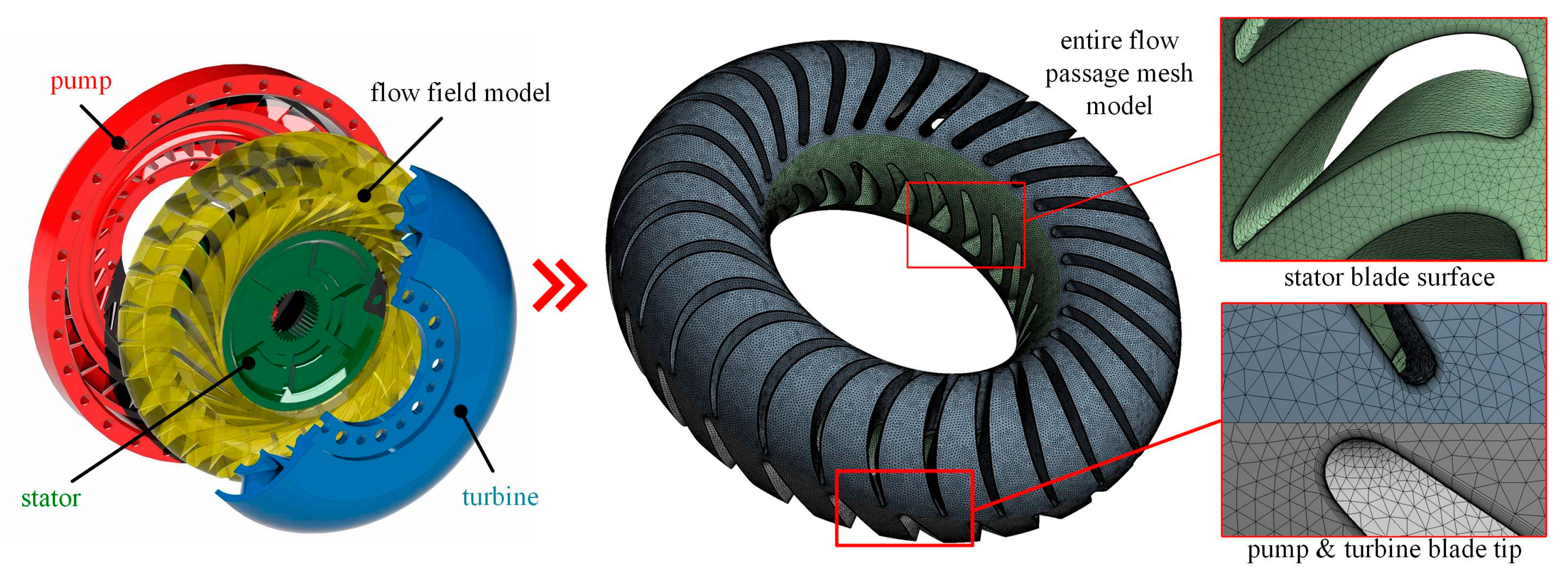
The full flow passage geometric model was extracted from a torque converter for construction machinery, the parameters of the torque converter are shown in

Table 2. Torque converter cascade parameters.

	Pump	Turbine	Stator
Blade number	29	25	22
Blade entrance angle (deg)	−31	46	−23
Blade exit angle (deg)	34	−65	50

. The pump, turbine and stator flow passages were discretized using unstructured tetrahedral elements in ANSYS Meshing. As the cavitation bubbles were generally small, a refined mesh around the blade is required to restore the real flow status and capture the cavitation flow behaviors (Figure 2).

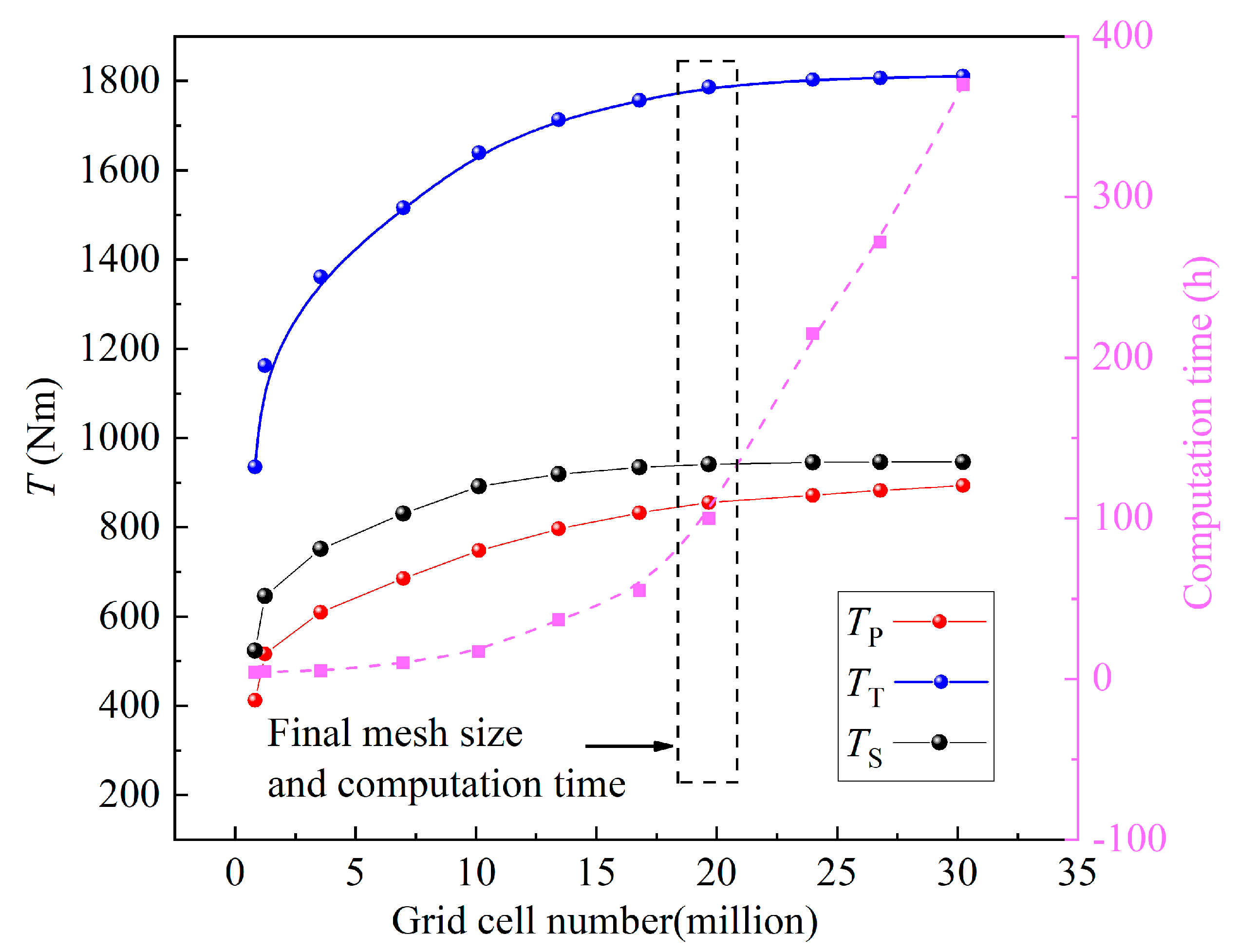
The accuracy and efficiency of the solution are directly affected by the mesh density. In theory, a higher grid number would yield better accuracy. However, a huge mesh number requires higher computing resources. Therefore, an appropriate mesh density should be determined by mesh independence analysis to achieve a proper balance between accuracy and computing cost, and the mesh model is considered independent if further refining the mesh produces less than 3% variation in results. A mesh independence test with WALE model was performed with different mesh resolutions; the reference pressure level was 0.4 MPa, the pump speed was 2000 rpm, and the turbine speed was fixed at 20 rpm. Figure 3 and

Table 3. Mesh independence study results.

Grid Cell Number (×106)	Computation Time (h)	TP (N m)	Div.	TT (N m)	Div.	TS (N m)	Div.
0.82478	4	412.13		935.38		523.24
1.23243	4.5	516.12	25.23%	1162.02	24.23%	645.90	23.44%
3.55688	5	609.69	18.13%	1361.08	17.13%	751.39	16.33%
6.98908	10	685.29	12.39%	1516.24	11.40%	830.95	10.59%
10.12353	17	747.79	9.12%	1639.36	8.12%	891.57	7.30%
13.43893	37	796.57	6.52%	1713.52	4.52%	918.95	3.07%
16.78994	55	832.52	4.51%	1756.58	2.51%	934.06	1.64%
19.67383	100	855.27	2.73%	1786.65	1.71%	941.39	0.78%
23.98664	215	871.78	1.93%	1803.11	0.92%	945.33	0.42%
26.79305	272	882.65	1.25%	1807.02	0.22%	946.37	0.11%
30.23543	370	893.42	1.12%	1811.02	0.22%	946.59	0.02%

shows the torque results of the pump, the turbine and the stator over variant mesh densities through the CFD calculation. Considering the computational efficiency and accuracy comprehensively, the element numbers of the pump, the turbine and the stator are 7,538,148, 6,319,448 and 5,442,091 respectively, and the pump torque variation is 2.73%, which satisfies the requirement for mesh independence.

2.4. Simulation Settings

Cavitation is difficult to converge due to the existence of a phase transition process with a complex turbulent structure; therefore, the study put forward a four-stage calculation process. Firstly, based on the first-order upwind scheme, the initial calculation of the cavitation-free internal flow field of the torque converter was carried out, and the circulation flow trend was obtained. Secondly, based on the low-precision initial value results, the high-resolution advection scheme was used to perform high-precision analysis on the turbulent structure of the cavitation-free flow field based on the SST turbulence model to obtain accurate turbulent flow results. At the same time, considering the stability and solution efficiency of multiphase flow calculation, the Stage interface boundary condition was used to transfer data between flow channels. Then, the Zwart cavitation model was applied to determine the steady-state cavitation status in the flow field, and the results were used as the initial value for transient calculations. Finally, the transient cavitation calculation was performed to capture the transient cavitation flow characteristics. In order to obtain the convergent solution of the highly unsteady cavitation flow, 5000 time steps were simulated to fully capture transient features. The details of the setting are shown in

Table 4. Detailed setting of torque converter CFD model.

Analysis Step	No Cavitation I	No Cavitation II	Cavitation III	Cavitation IV
Analysis type	Steady state	Steady state	Steady state	Transient
Advection scheme	Upwind	High resolution	High resolution	High resolution
Interface model	Frozen rotor	Frozen rotor	Stage	Transient Rotor-Stator
Cavitation model	None	None	Zwart model	Zwart model
Time step	1 × 10−3 s	1 × 10−4 s	1 × 10−4 s	1 × 10−5 s
Step number	300	300	400	5000
Convergence target	RMS 1 × 10−4	RMS 1 × 10−5	RMS 1 × 10−5	RMS 1 × 10−5
Fluid properties	ρf = 835.2 kg·m−3, μf = 1.46 × 10−2 Pa·s
Vapor properties	ρg = 2.1 kg·m−3, μg = 1.2 × 10−5 Pa·s
Pump status	NP = 2000 rpm
Turbine status	NT = 20−1800 rpm
Stator status	NS = 0
Reference pressure	pref = 0.4 MPa
Boundary details	No-slip and smooth wall

.

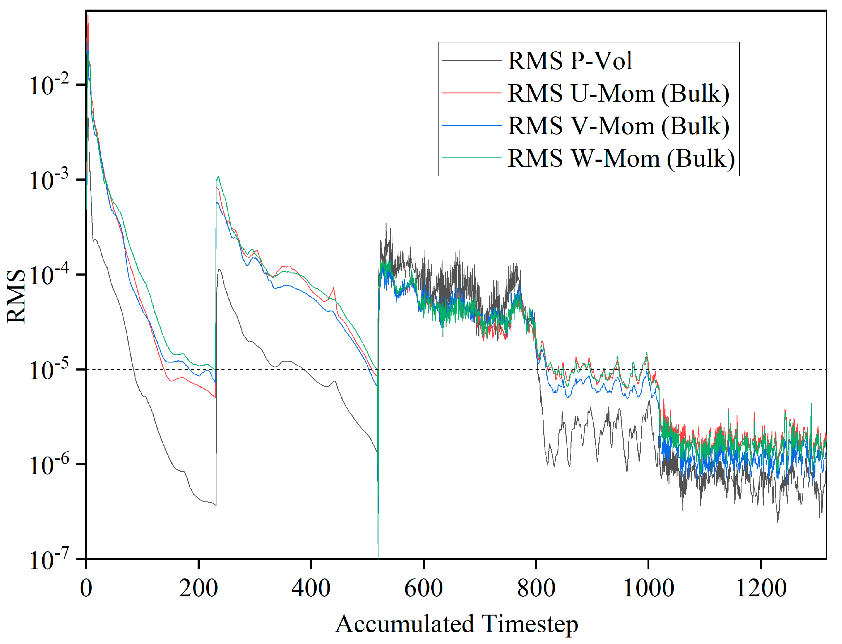
The convergent results of the generated mesh show that the numerical results converge to RMS < 1 × 10⁻⁵ (Root Mean Square) quickly, with WALE model in stall condition (SR = 0.01), as shown in Figure 4.

3. Hydraulic Torque Converter Test Rig

3.1. Hydrodynamic Performance Test of Hydraulic Torque Converter

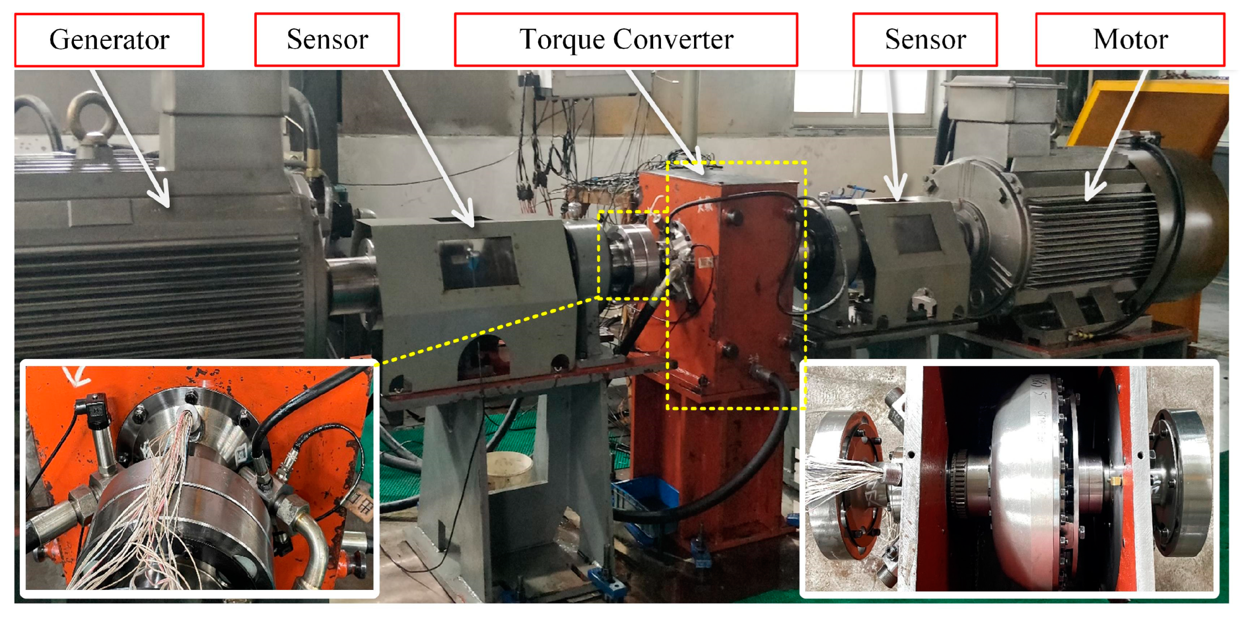
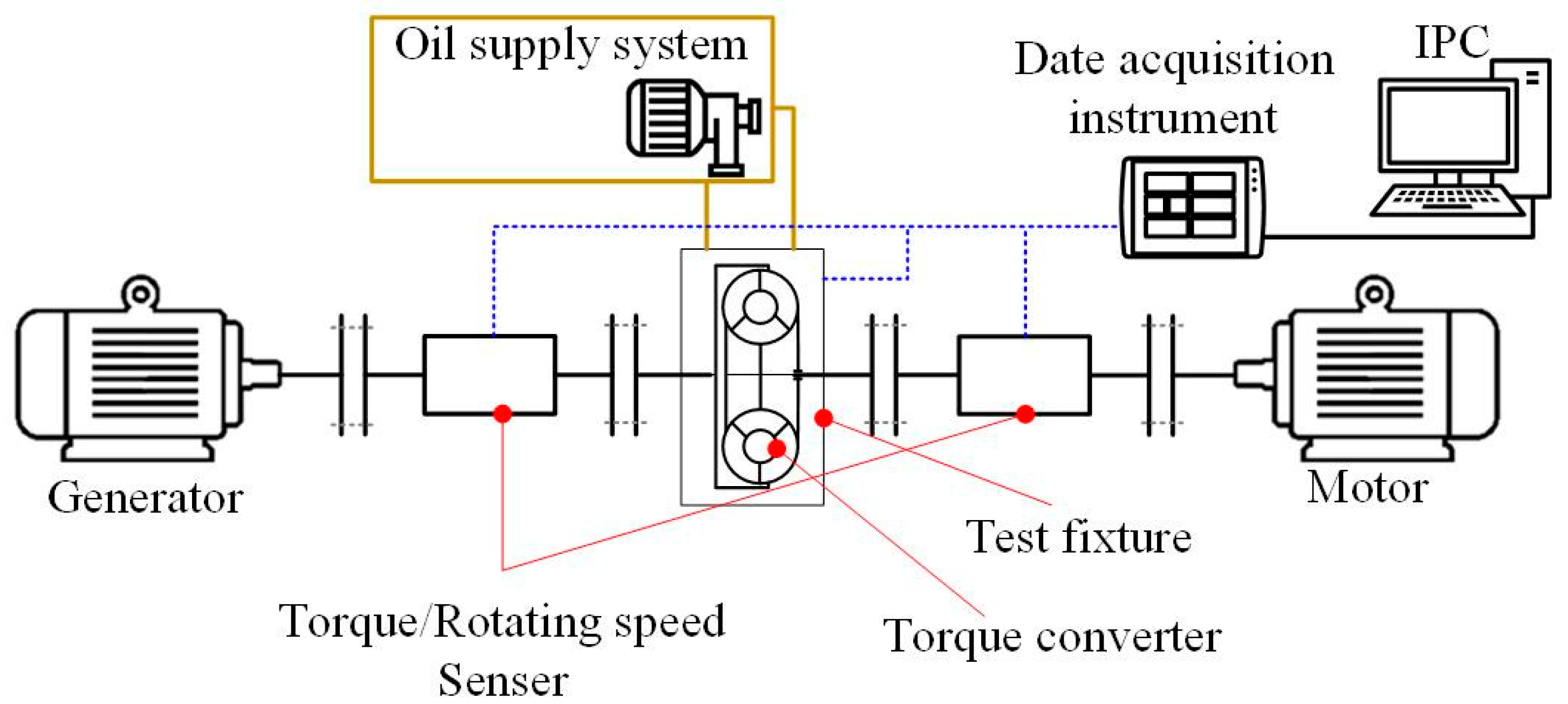
Two high-power motors were adopted as the torque converter input (300 kW) and the loading device (500 kW). The speed and torque sensors were installed at the input and output ends of the torque converter, respectively, with a calibration accuracy of 0.5%. The torque converter test fixture was supplied with oil by an independent hydraulic pump station system, which can realize the adjustment of the charging oil pressure at the inlet and outlet. The inlet and outlet of the torque converter were equipped with high-precision pressure and temperature sensors, which can monitor the oil conditions during operation. The structure of the test bench is shown in Figure 5 and Figure 6.

3.2. Blade Surface Pressure Test Inside Hydraulic Torque Converter

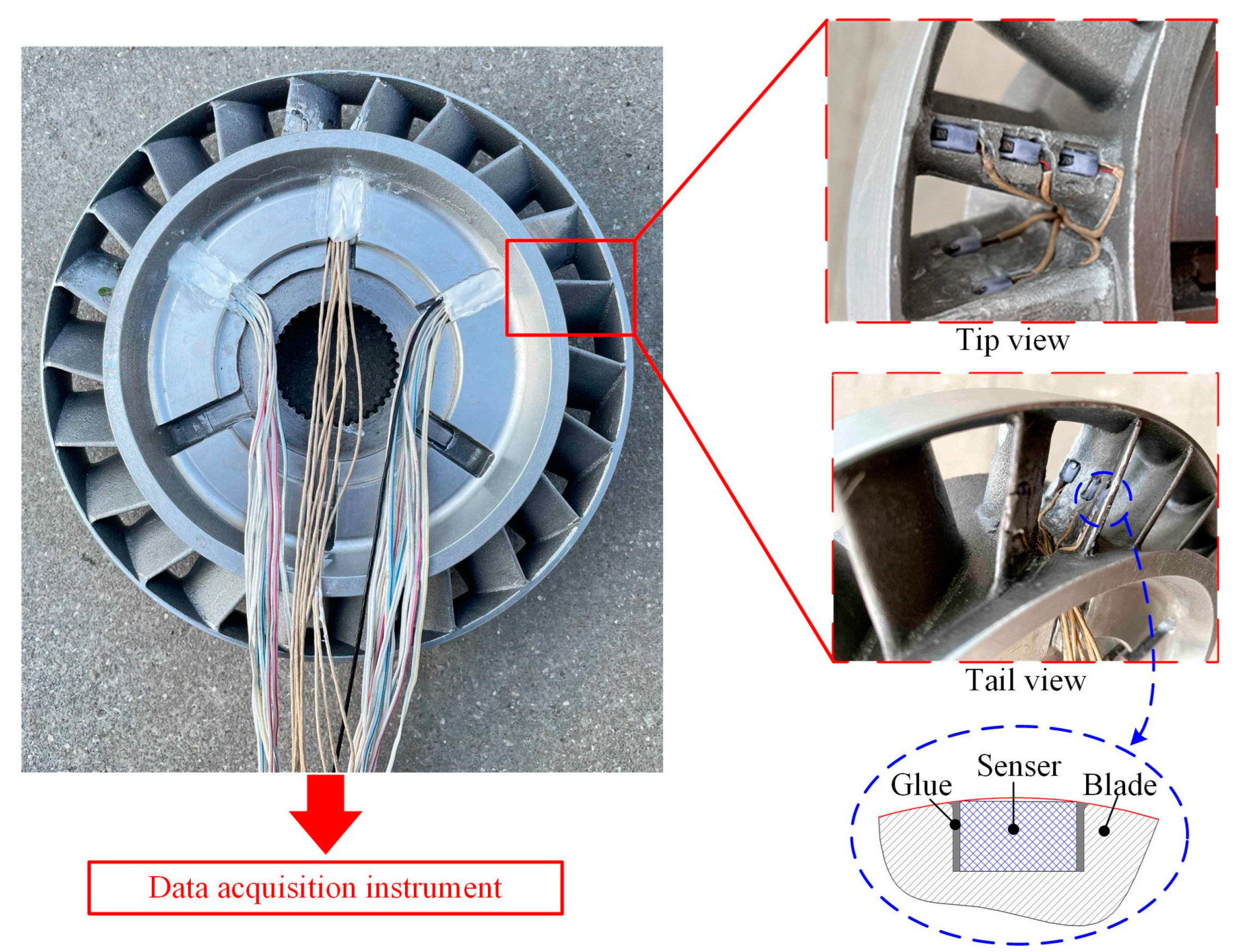
Based on the performance test system of the torque converter, the stator blade surface pressure measurement system was established and shown in Figure 7. The sensor installation slots were cut on the surface of the tested stator blade, and the ultra-small dynamic pressure sensors and the wires were fixed in the slot with glue to avoid interference with the main flow. The gaps were filled with glue to ensure the tightness and smoothness of the installation. In order to reduce the interference of ambient signals, low-impedance conductors with frequency closed layers are applied, and the voltage signal is led to the signal collection device and converted into a dynamic data-to-pressure value signal [41]. The measurement accuracy of the dynamic absolute pressure signal of the sensor is higher than ±0.1%.

4. Results

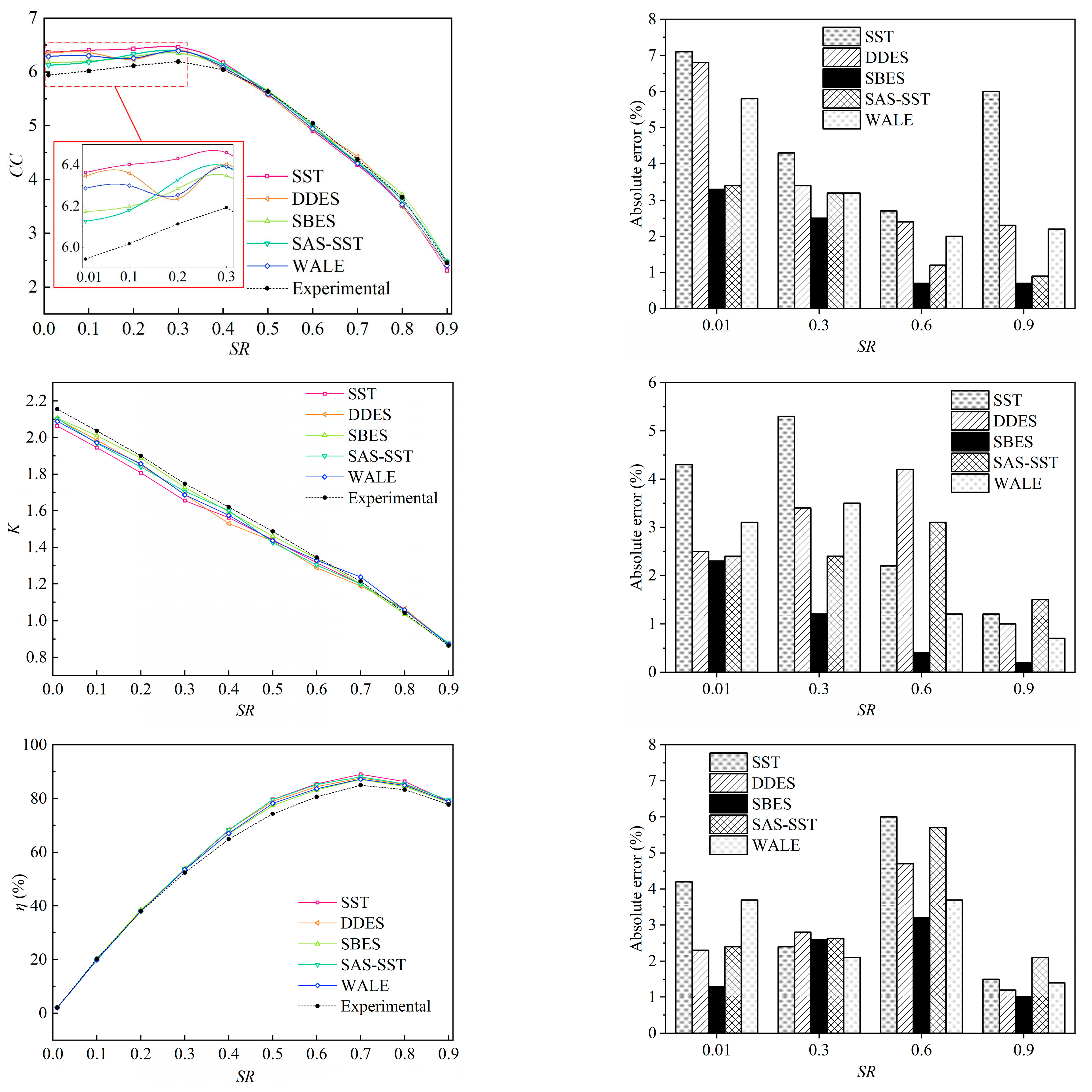
Three hydrodynamic performance indicators are generally used to evaluate the performance of the torque converter: torque ratio, capacity factor and efficiency. The hydrodynamic performance of a torque converter is defined by several operating parameters that are described as follows.

$$SR=\frac{N_{\mathrm{T}}}{N_{\mathrm{P}}}$$

(28)

$$K=\frac{T_{\mathrm{T}}}{T_{\mathrm{P}}}$$

(29)

$$\eta =\frac{N_{\mathrm{T}}\times T_{\mathrm{T}}}{N_{\mathrm{P}}\times T_{\mathrm{P}}}=SR\times K$$

(30)

$$CC=\frac{T_{\mathrm{P}}}{\rho g{N}_{\mathrm{P}}{}^2{D}^5}$$

(31)

where N_P and N_T represent the rotating speed of the pump and turbine, SR is the speed ratio, T_P, T_T, and T_S represent pump torque, turbine torque, and stator torque, respectively.

As shown in Figure 8, from the error evaluation point of view, the errors between the three indicators and the experimental data are small, and the maximum error is less than 8%, indicating that the simulation is basically consistent with the experiment, and further illustrates the validity and reliability of the numerical simulation. As shown, the calculation results of the three hydrodynamic performance characteristics of the SRS models under multiple operating conditions all show higher accuracy than the SST model. In particular, SST model shows higher accuracy than DDES and SAS-SST but lower than SBES for the prediction of torque ratio for high-speed ratios. Among them, SBES has higher accuracy than other models under multiple working conditions, and the accuracy range is 0.2~3.9%. SBES and SAS-SST exhibit higher characteristic prediction accuracy under stall conditions, the capacity constant errors of SBES and SAS-SST models are 3.3% and 3.1%, the torque ratio and efficiency errors of SBES are 2.3% and 1.3%.

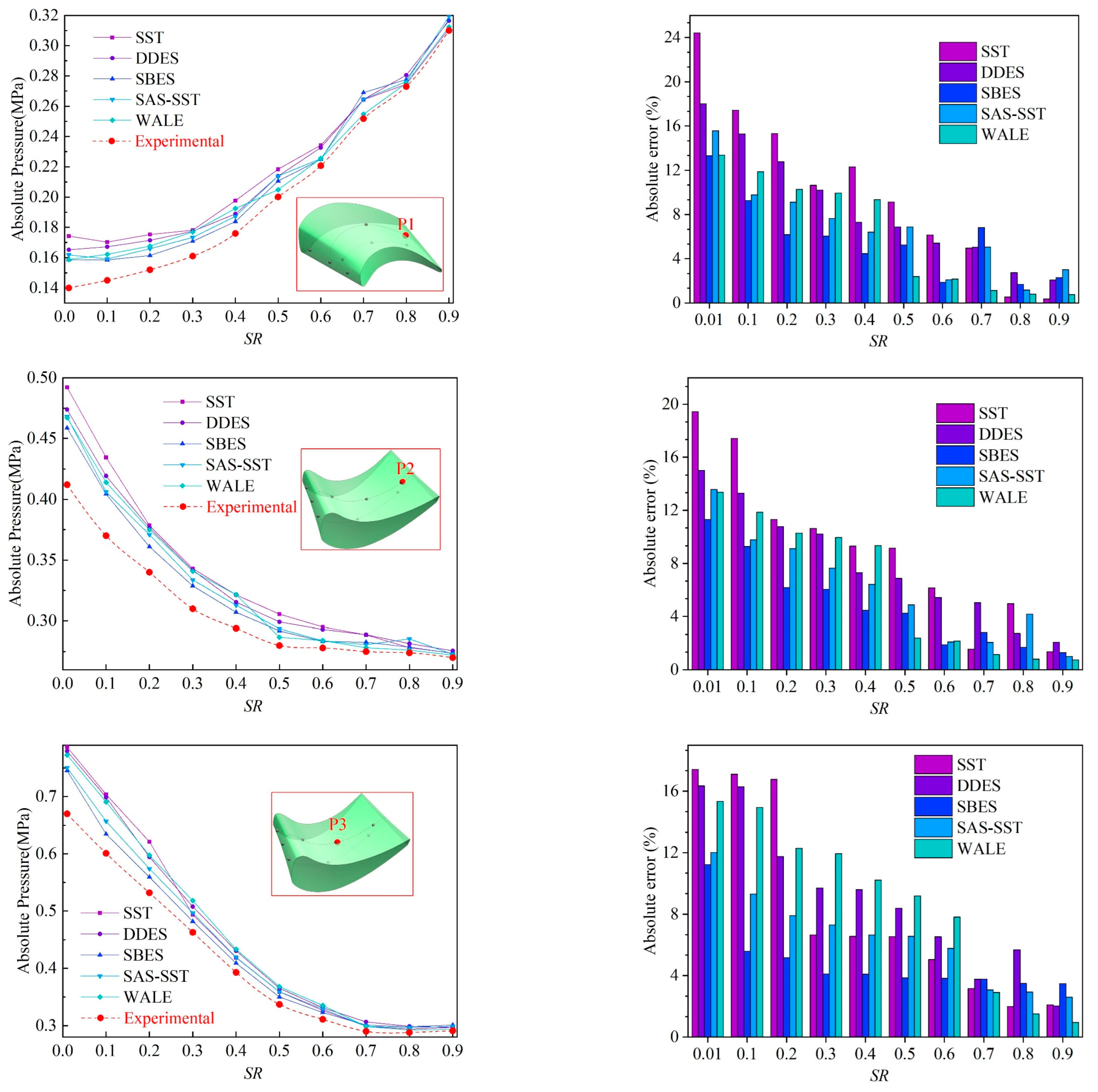
In this paper, pressure measurement data with long sampling times and high signal-to-noise ratios were selected. The absolute pressure at P1 (on the suction side near the tail), P2 (on the pressure side near the tail) and P3 (on the pressure side in the middle) was analyzed and compared with the calculation results using different turbulence models.

As shown in the Figure 9, the variation trend in the absolute pressure at the measuring point with the speed ratio is the same for different turbulence models. With the increase in the speed ratio, the back pressure of the stator blade increases, the abdominal pressure decreases, and the pressure difference of the absolute pressure on the blade surface decreases. The prediction accuracy based on different models increases with the speed ratio. Compared with the SST model, the prediction accuracy of the absolute pressure of the blade surface measuring points under the low-speed ratio of the torque converter using SRS is significantly improved. The maximum error of the SST model reaches 24.43% at P1 during stalling. The SBES model has the highest average pressure prediction accuracy under multiple operating conditions, while the average errors of different measuring points are 5.72% (P1), 4.92% (P2), and 4.86% (P3). The largest error of the SBES model also occurs during startup, which is 13.32% at the P1 measuring point.

5. Flow Field Analysis

5.1. Overall Cavitation Characteristics

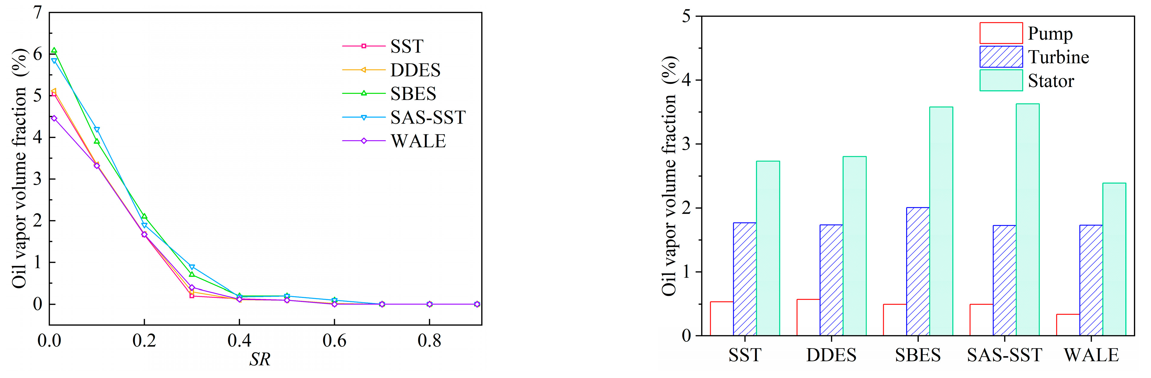
From the total volume fraction of the vapor bubbles in the flow field at different speed ratios in Figure 10, it can be seen that the cavitation bubbles occur under low SR range and vanish when SR is higher than 0.4, and the cavitation degree reaches its maximum when stalling (SR = 0.01). Thus, the following sections mainly analyze the flow field under the stall operating condition. The results show that simulated vapor volume values of the SBES and SAS-SST models are larger than those of the SST, DDES and WALE models under usual operating conditions. SST, DDES and WALE predictions show that the maximum vapor volume fraction drops below 10% when SR is higher than 0.3, indicating the dissidence of cavitation. However, SBES and SAS-SST results show that cavitation will not disappear until SR is higher than 0.4. When stalling, SBES and SAS-SST models also show a higher vapor volume fraction in the stator domain than the other models.

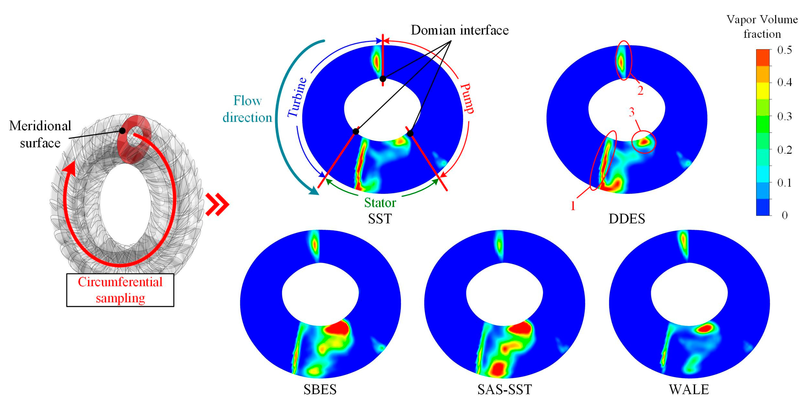
In order to characterize the overall distribution of cavitation vapor in the flow field, the vapor volume fraction was averaged and shown in meridional surface. As in Figure 11, it can be found that for all turbulence models, the cavitation vapor is mainly distributed at the middle of the blade tip in the turbine and stator (area 1), and a small amount of vapor is distributed in shroud side of blade tip in the pump (area 2). However, different cavitation regions were determined by the selected turbulence models. The SST and DDES models show that vapor became centralized at the stator blade tip. As for the SBES, SAS-SST and LES models, the vapor is mainly distributed at hub side area of blade tail (area 3).

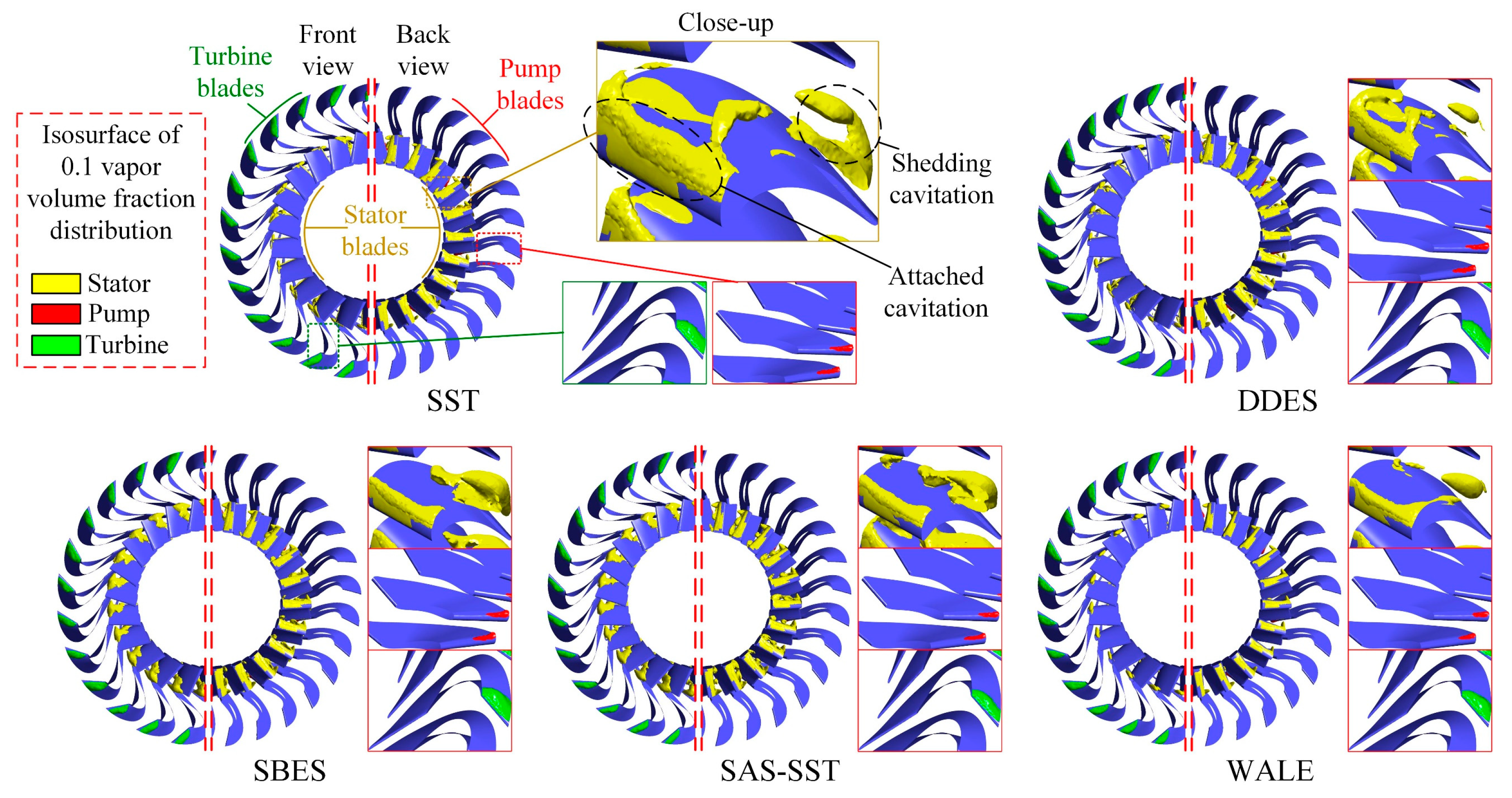
The time-averaged results of the cavitation transient simulation are shown in Figure 12. The application of different turbulence models has a significant effect on the overall distribution of cavitation. In the turbine domain, stable attached cavitation bubbles mainly occur at the tip of the blade near the inlet. In the pump domain, a small range of attached cavitation could be found at the inlet end of the impeller blade near the shroud side. In the stator flow field where cavitation is the most serious, large-scale attached cavitations were found on the blade tip, and different degrees of shedding cavitation bubbles could also be detected on the suction side of the blade. It can be seen from the figure that the SST and DDES models yield larger attached cavitation areas at the blade tip than other models. The simulation results of the SAS-SST and SBES models show a larger cavitation shedding volume, and the shedding cavitation area is mainly distributed in the middle of the flow channel near the hub side. The cavitation distribution characteristics of WALE are between the above two types of models.

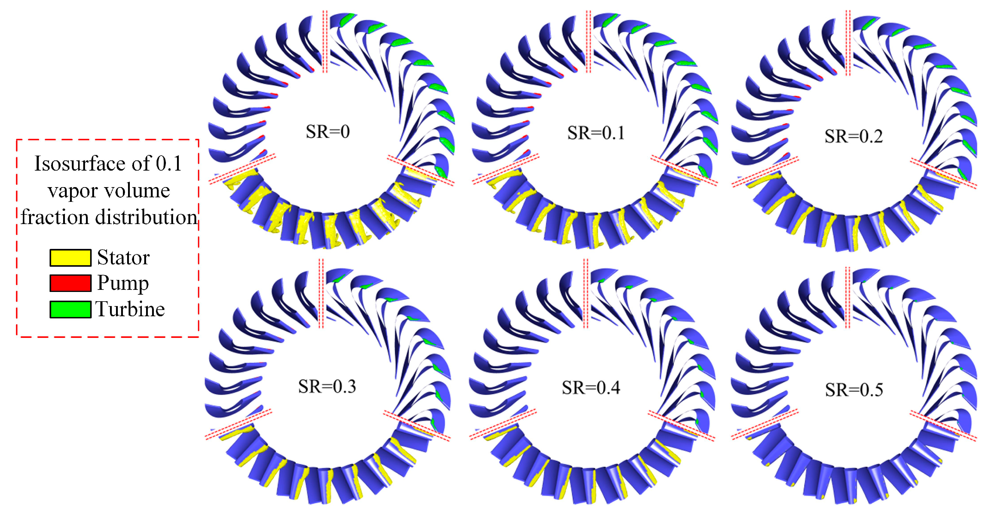
Figure 13 shows the vapor volume fraction distribution in the impellers with SBES model in different operating conditions. The cavitation bubbles in the turbine and stator domains decreased as the turbine rotation speed increased. When SR ≥ 0.3, no measurable cavitation can be found in the pump because of the decreased mass flow rate. When SR ≥ 0.4, the cavitation bubbles dissolved in the turbine. When SR ≥ 0.5, no cavitation bubbles were generated in all fluid domains. Stable attached cavitation developed in the pump and turbine under all operating conditions; however, the cavitation inside the stator flow field was transient and more complicated.

5.2. Cavitation and Vortex Analysis of the Chord Surface

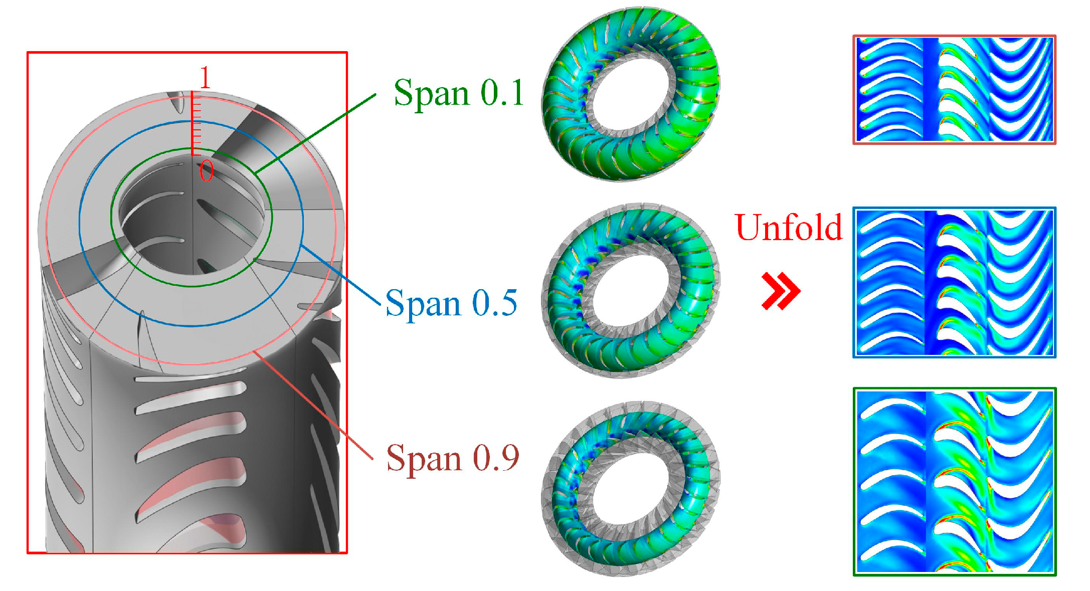
In this section, three representative chord surfaces in the span direction are chosen to analyze the vortex and vapor volume fraction distribution, and the position of the chord surface is shown in Figure 14. In the figure, 0–1 represents the relative dimensionless distance between the hub and the shroud, where Span 0.1, Span 0.5, and Span 0.9 represent the span surface near the hub, in the middle and near the shroud, respectively.

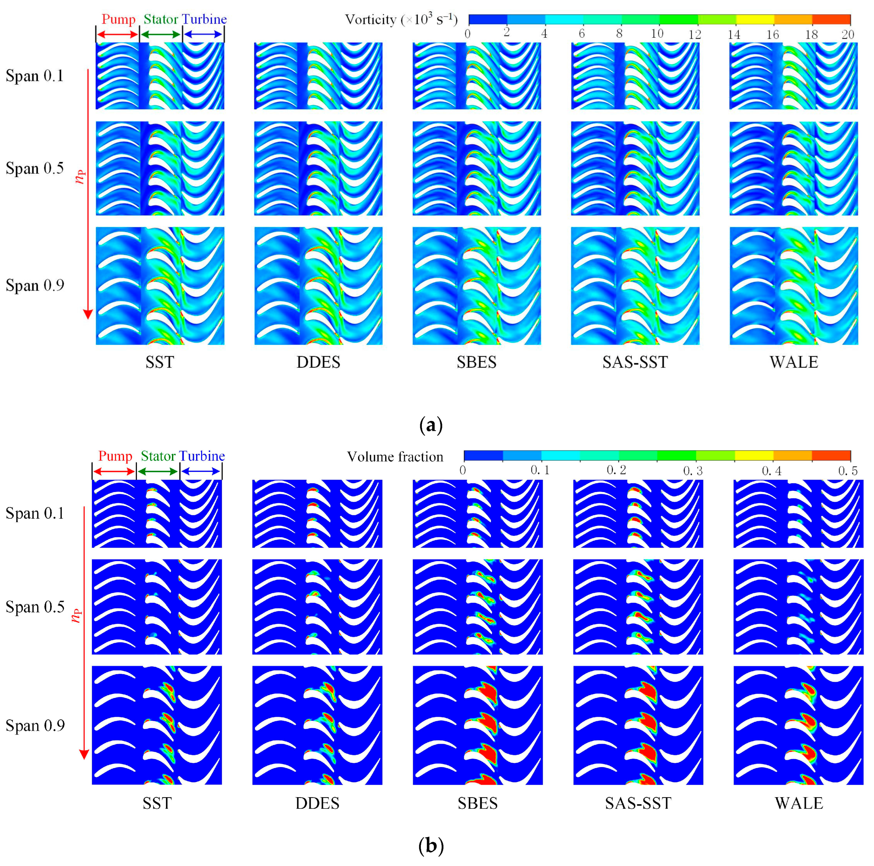
Figure 15 shows that large vortex zones exist near the blades, especially at the tip of stator blades where the fluid velocity is large. The simulated vortex values of the SBES and SAS-SST models are larger than those of the SST, DDES and WALE models, indicating that larger vortices are captured in the SBES and SAS-SST simulations. The result shows that the energy dissipation loss of the SBES and SAS-SST models is larger than those of the SST, DDES and WALE models because of viscous dissipation, which could be the reason why SBES and SAS-SST torque errors are smaller than others under the stall operating condition.

From the bubbles volume fraction of the three surfaces in Figure 15b, it can be found that the vapor volume fraction of the span 0.5 surface is larger than other surfaces, indicating that a large number of bubbles exist in the corresponding area. The results indicate that the higher cavitation degree can cause larger vorticity viscous dissipation.

5.3. D Vortex Structure in the Stator Flow Field

The vortex structure changes with the appearance of cavitation. Therefore, analyzing the vortex characteristics of cavitation is important for the understanding of torque converter cavitation. In order to accurately capture the vortex structure of the flow field, the Q criterion is introduced to evaluate the vortex structure in the internal flow field, which is defined by

$$\mathrm{Q}=\frac{1}{2}\left(\parallel \mathsf{\Omega }{\parallel }^2-\parallel \mathrm{S}{\parallel }^2\right)$$

(32)

where Ω (vortex tensor) and S (strain rate tensor) are the antisymmetric and symmetric portions of the velocity gradient tensor, respectively.

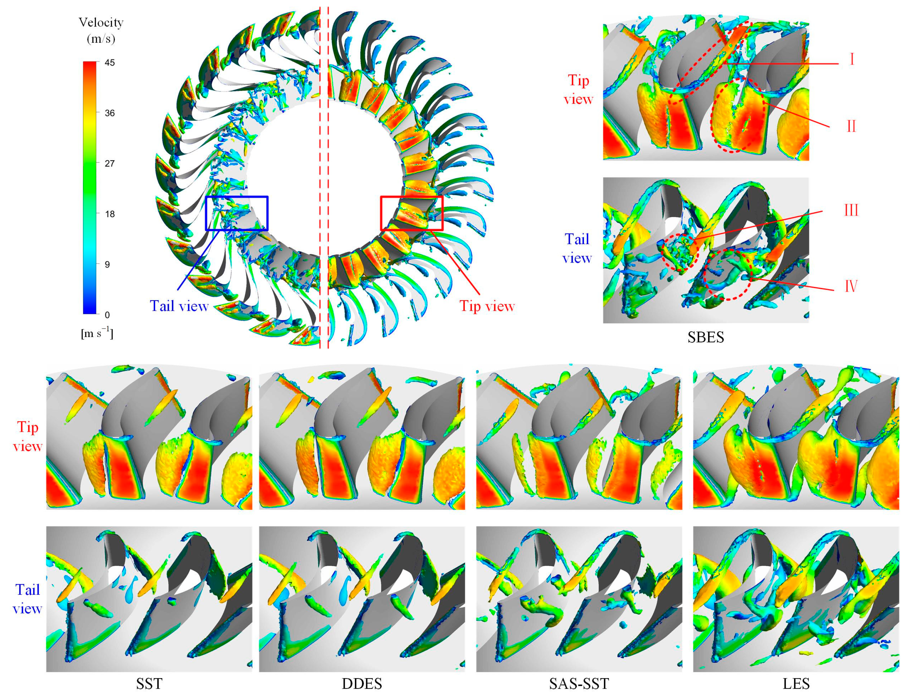
To obtain a better resolution of the vortex structure, iso-surfaces with Q = 4.5608 × 10⁶ s⁻² are shown in Figure 16, and local velocity values on the vortex core surface are marked with a different color. Large-scale wall vortex (WV) and shedding separation vortex (SV) could be found at the tip of the stator blade where attached cavitation occurs, and the WALE model results exhibit the largest wall vortex range. Passage vortex (PV) can be detected near the hub, and the vortex of WALE and SBES is the strongest. The SAS-SST, SBES and WALE models also captured horseshoe-shaped vortices at the tail of the blade, and the vortex structure of SAS-SST is more obvious. In addition, a dense small vortex concentration area was also captured in the simulation results of the SBES model, which may be caused by the disappearance of cavitation.

5.4. Quantitative Analysis of Blade Pressure

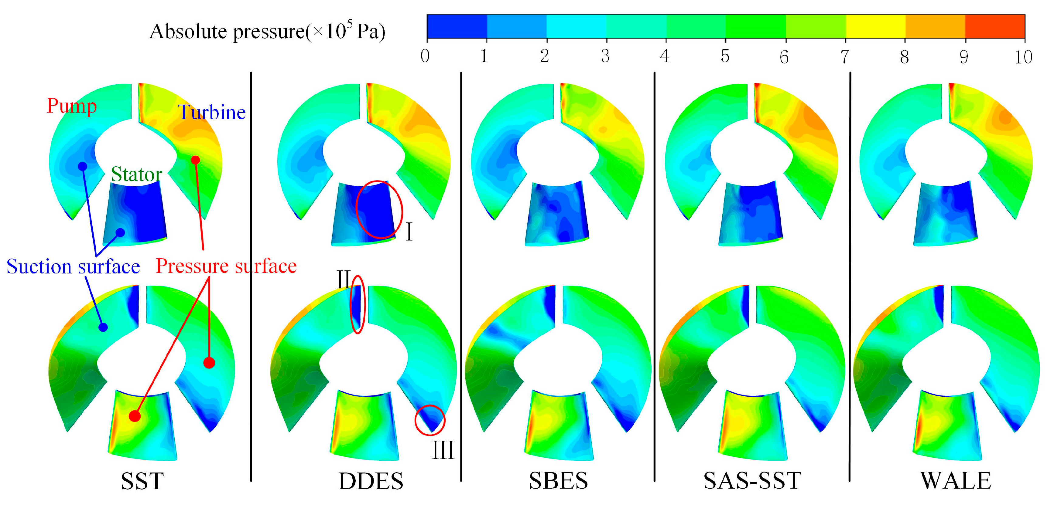
As shown in Figure 17, low-pressure areas could be found near the cavitation zones. Due to centrifugal force, the relatively high-pressure area of the pump blade is distributed near the shroud side, and the pressure difference between the suction surface and the pressure surface is relatively small, resulting in cavitation potential. A steep low-pressure region is created in the corresponding region II due to the presence of stable attached cavitation with a high vapor volume rate at the turbine blade tip. The average pressure on the suction side of the stator blades is lower in the SST and DDES results due to poor prediction of cavitation shedding. It can be found that when the degree of shedding cavitation is greater than that of attached cavitation, the surface pressure difference of the blade is lower, and this conclusion has guiding significance for the cavitation control of torque converter.

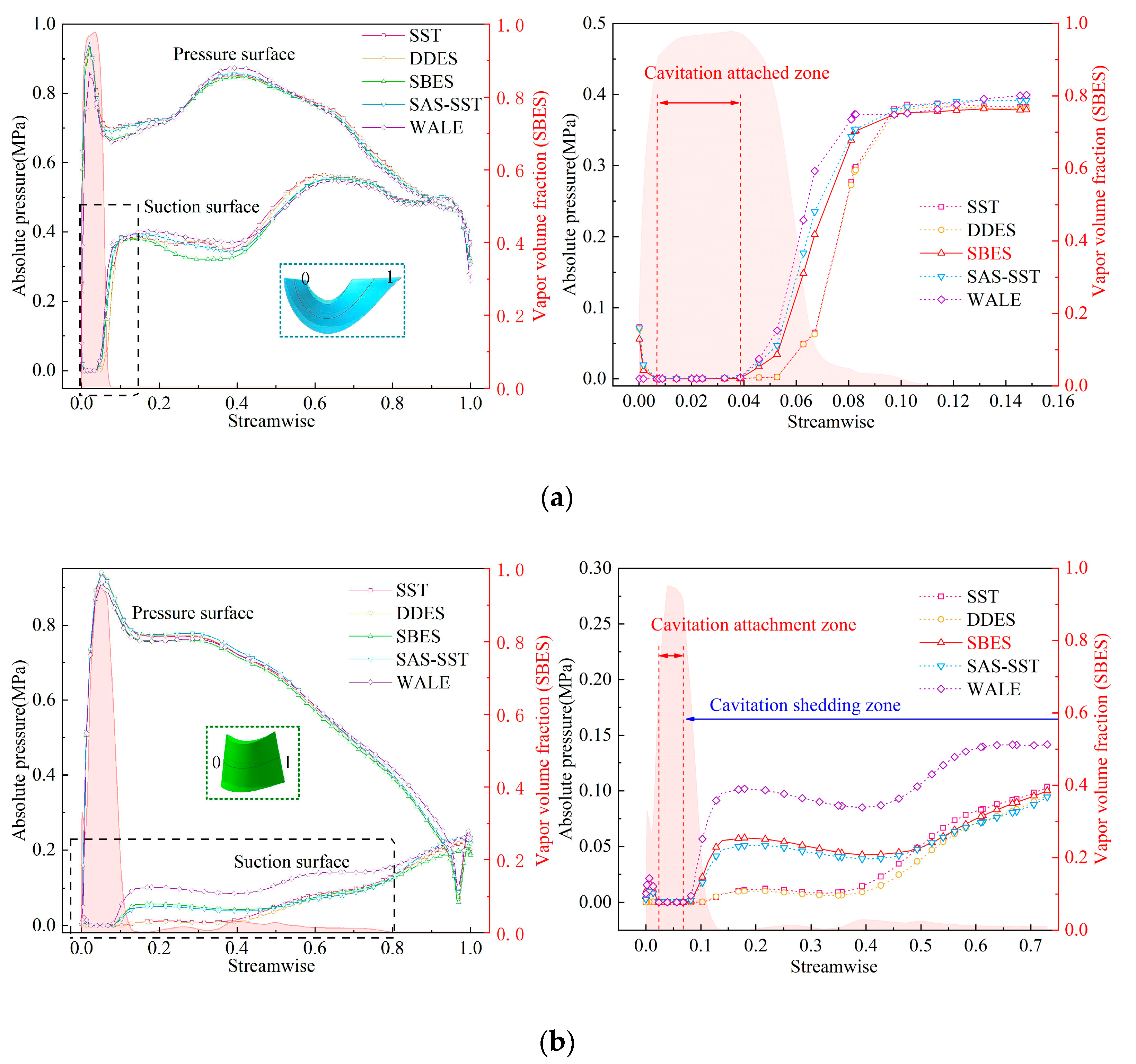
The computational absolute pressure distribution along the middle streamwise direction with different models is shown in Figure 18. Taking the vapor volume fraction along the streamwise direction of the SBES model result as an analysis reference, there is little difference in the streamwise pressure results with regard to the turbine and the pressure surface of stator. On the suction surface of the blade, different models have different prediction results on the occurrence degree and evolution state of cavitation, and the corresponding pressure distribution is also different.

A low-pressure region is generated in the turbine blade tip. The cavitation attachment region is generated in the 0.007–0.038 streamline position. On the suction surface of the stator, the cavitation attachment area is located at 0.024–0.075 in the streamwise direction. A comparative analysis with Figure 15 shows that due to the difference in the prediction results of shedding cavitation, the pressure distribution on the blade surface corresponding to the region shows different characteristics. The SBES and SAS-SST models fully predict the shedding cavitation, and the local pressure is greater than that of SST and DDES. The results of the WALE model show that the cavitation bubbles are completely detached and are far away from the wall, corresponding to the maximum pressure in the cavitation detachment area. Therefore, the blade surface load is the result of the interaction between the vapor volume rate (the degree of cavitation) and the type of cavitation in the flow field. Comparing with shedding cavitation, attached cavitation can reduce the average pressure on the suction surface of the blade and hence increase the lift of the blade to a certain extent; this conclusion has guiding significance for the optimal design of airfoil considering cavitation.

6. Analysis of Transient Cavitation Evolution in the Stator

Heavy cavitation was predicted in the stator under stall operating conditions, and only stable sheet cavitation was detected in the turbine. It was proven that the SBES model showed higher accuracy in the prediction of both overall hydrodynamic performance and averaged flow field pressure characteristics. The transient cavitation flow characteristics of the stator based on SBES are illustrated and validated as follows.

6.1. Spectral Analysis of Vapor Volume and Pressure

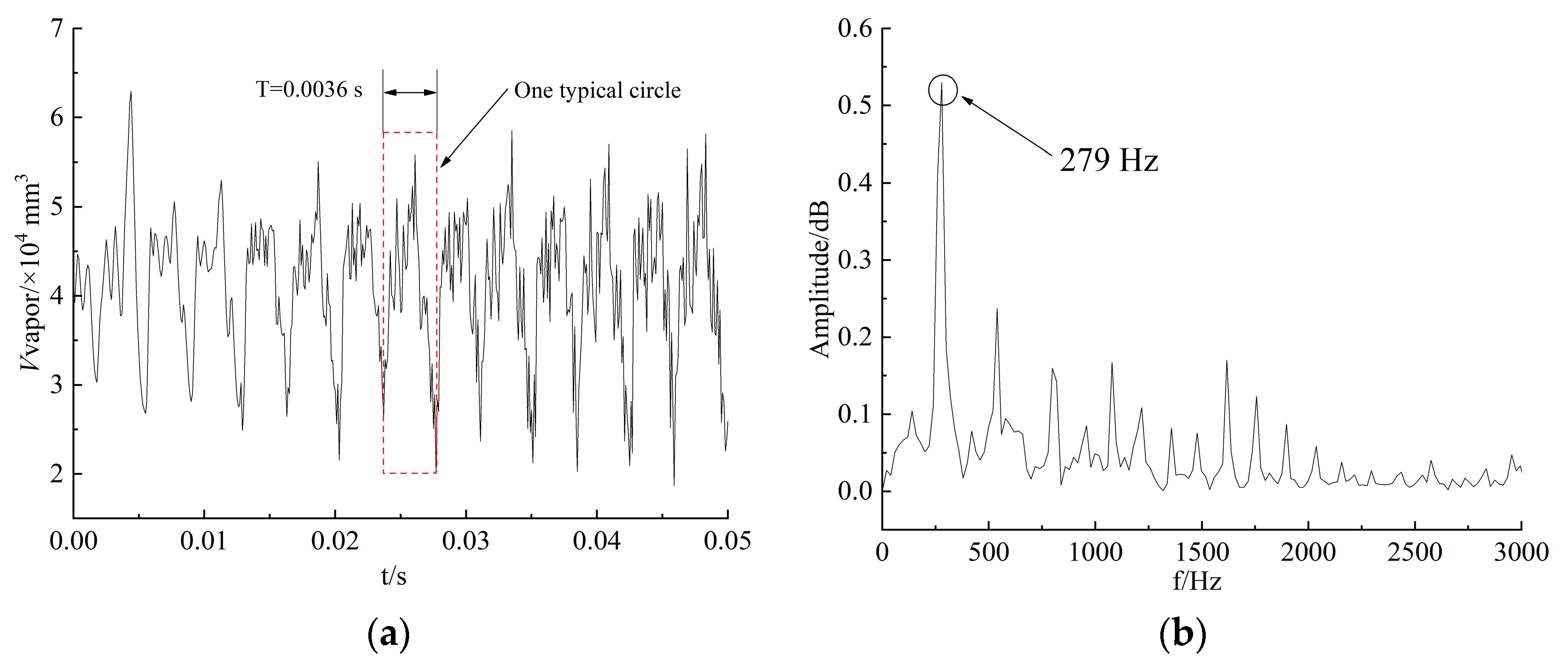
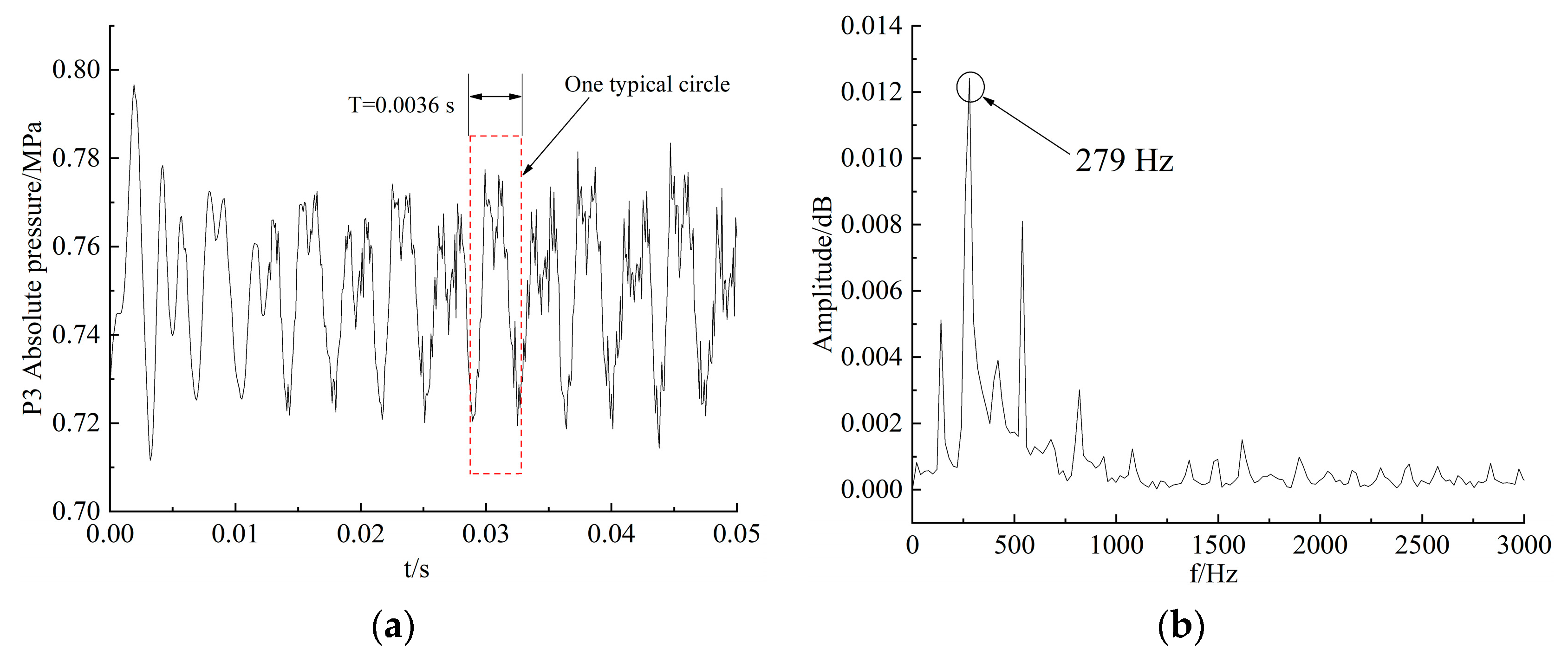
In the stator, the evolution of the cavitation flow can be illustrated by the time history of the vapor volume. As shown in Figure 19 and Figure 20, the change in vapor volume is periodic due to the occurrence of cavitation shedding in the flow channel. The predicted frequency of cavitation evolution is about 279 Hz. Periodic cavitation results in a 4 × 10⁴ mm³ change in vapor volume in the stator domain, which reduces hydraulic performance. The change frequency of the vapor volume is in good agreement with the frequency of the absolute pressure at the P3 measuring point, indicating that the cavitation flow causes the fluctuation of the flow pressure in the stator. According to the time-frequency analysis results, the evolution period of cavitation bubbles is 0.0036 s. The results show that the dynamic pressure characteristics of the internal flow field can effectively identify the cavitation characteristics. However, it is worth noting that such frequency reflects the periodic shedding behavior of cavitation bubbles rather than the forming and collapsing of one single bubble, which evolves with a much higher frequency.

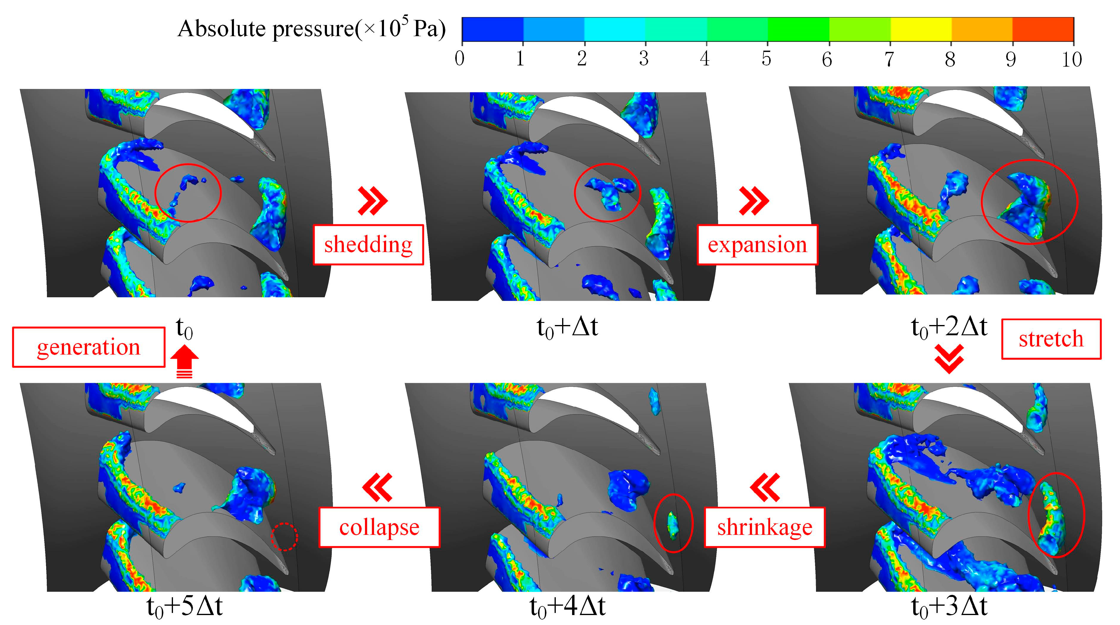
6.2. Evolution of Cavitation

According to the spectral analysis results, the transient cavitation process of the flow field in the stator is periodic. The isosurface of vapor volume fraction 0.1 is constructed to capture the cavitation shape, and the surface pressure characteristics of the cavitation bubbles are analyzed as shown in Figure 21. Two distinct transient cavitation signatures are captured. Under the high-speed flow impact from the turbine, an attached cavitation region forms at the tip of stator blade on the other hand, the shedding cavitation bubbles are determined at the tip of the blade close to the hub. Cavitation bubbles shed off from the attached cavitation region and form an independent cavitation area. Then it moves downstream with the main liquid flow, and cavitation bubbles expand continuously during this process. After entering the high-pressure region in the blade tail, the cavitation bubbles are compressed and stretched into a rod shape, the volume is continuously reduced, and finally collapses and disappears.

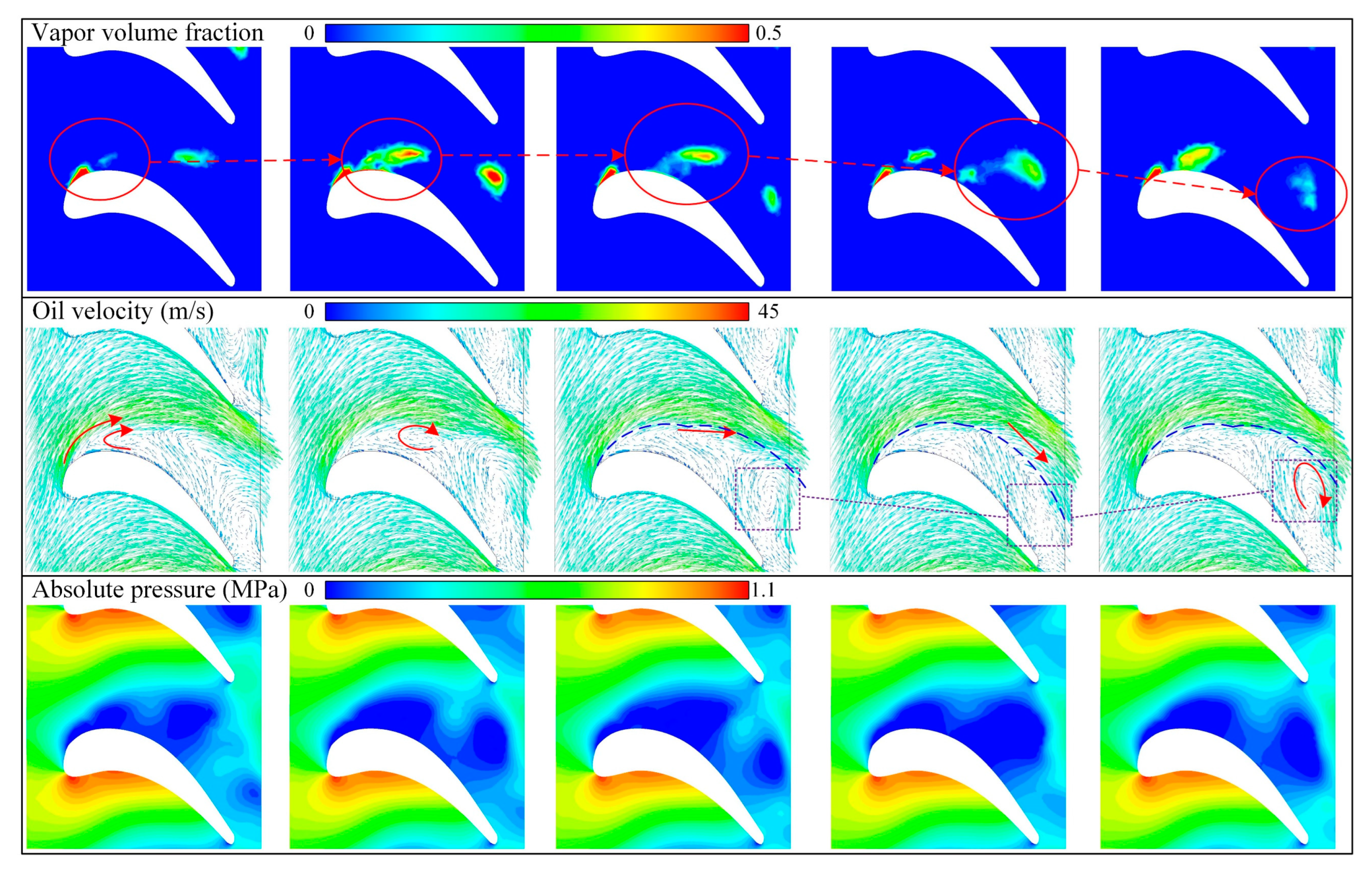
6.3. Transient Shedding Cavitation Flow Analysis

The vapor volume fraction, oil velocity vector and absolute pressure in one typical cavitation bubble evolution cycle are analyzed and shown in Figure 22. As a result of the high-speed impact of the turbine flow, transient cavitation bubbles are initially formed in the low-pressure region near the blade tip on the suction side, and a separation flow is formed on the suction side of the stator blade tip area corresponding to the WV and SV regions in Figure 16. The oil was torn apart and vapor levels rose as the local pressure dropped below the vapor pressure. Under the interaction of the re-entrant jet and incoming flow, the bubbles broke and shed from the blade surface and moved towards the tail of the blade. During the movement, the vapor condensed, the gas content of the bubbles decreased, and the large vortex at the tail disappeared with the condensation of the bubbles.

7. Conclusions

SRS and SST turbulence methods were compared and validated through test data to improve torque converter cavitation performance prediction accuracy and provide understanding of the flow structure. The following conclusions are drawn:

(1) SRS shows better prediction accuracy in terms of both hydrodynamic characteristics and internal pressure levels. The SBES model shows higher accuracy under multiple working conditions, whose error rate ranges from 0.2% to 3.9%. At stall conditions when the cavitation reaches the peak, the capacity constant prediction error of SBES and SAS-SST model is lower than 3.4%, while the torque ratio and efficiency of SBES errors are 2.3% and 1.3%, respectively.

(2) The time-averaged simulation results of transient cavitation flow fields in the three impellers using different turbulence models show similar overall distribution laws. The most serious cavitation occurs in the stator, followed by turbine and pump. The difference in the occurrence of cavitation is closely related to the distribution of eddy viscosity in the flow field and the characteristics of the vortex structure. The ability of the SRS model to capture the vortex structure improves its cavitation prediction accuracy.

(3) SRS generally shows better prediction accuracy of wall absolute pressure than RANS according to the test results. The SBES model has the highest simulation accuracy at different pressure measurement points under multiple operating conditions, and the largest error occurs at the P1 measurement point under stall conditions, where the error value is 13.32%.

(4) Based on the transient cavitation results predicted by SBES, the cavitation process of the stator flow field in the torque converter is highly unsteady. It occurs in the stator blades tip, evolves in the flow channel near the hub side, and collapses and disappears near the outlet of the flow channel. The evolution process of cavitation bubbles in the stator is driven by the spatial distribution of pressure. Periodic processes can be captured by flow field vapor volume and pressure changes of the wall measuring point; the evolution period of cavitation bubbles in the stator is about 0.0036 s.

While the scale-resolved simulations provide high-precision flow field and accurate characteristic results, the cost of computational cost is still very high, which requires further optimization of the computational model. Meanwhile, in order to fully evaluate the performance of TC, a multi-objective optimization design of the wheel sets considering cavitation is needed to improve torque capacity and transmission efficiency.

References

- Ran, Z.; Ma, W.; Liu, C. 3D Cavitation Shedding Dynamics: Cavitation Flow-Fluid Vortex Formation Interaction in a Hydrodynamic Torque Converter. Appl. Sci. 2021, 11, 2798. [Google Scholar] [CrossRef]
- Yin, Z.; Gu, Y.; Fan, T.; Li, Z.; Wang, W.; Wu, D.; Mou, J.; Zheng, S. Effect of the Inclined Part Length of an Inclined Blade on the Cavitation Characteristics of Vortex Pumps. Machines 2023, 11, 21. [Google Scholar] [CrossRef]
- Liu, C.; Guo, M.; Yan, Q.; Wei, W. Influence of Charging Oil Condition on Torque Converter Cavitation Characteristics. Chin. J. Mech. Eng. 2022, 35, 49. [Google Scholar] [CrossRef]
- Ran, Z.; Ma, W.; Liu, C. Design Approach and Mechanism Analysis for Cavitation-Tolerant Torque Converter Blades. Appl. Sci. 2022, 12, 3405. [Google Scholar] [CrossRef]
- Guo, M.; Liu, C.; Yan, Q.; Wei, W.; Khoo, B.C. The Effect of Rotating Speeds on the Cavitation Characteristics in Hydraulic Torque Converter. Machines 2022, 10, 80. [Google Scholar] [CrossRef]
- Pan, X.; Xinyuan, C.; Hongjun, S.; Jiping, Z.; Lin, W.; Huichao, G. Effect of the blade shaped by Joukowsky airfoil transformation on the characteristics of the torque converter. Proc. Inst. Mech. Eng. Part D J. Automob. Eng. 2021, 235, 3314–3321. [Google Scholar] [CrossRef]
- Ghadimi, A.; Ghassemi, H. Comparative assessment of hydrodynamic performance of two-dimensional Naca0012 and Naca6612 hydrofoils under different cavitation and non-cavitation conditions. Int. J. Hydromechatronics 2020, 3, 349–367. [Google Scholar] [CrossRef]
- Yang, K.; Liu, C.; Li, J.; Xiong, J. Calculation and analysis of thermal flow field in hydrodynamic torque converter with a new developed stress-blended eddy simulation. Int. J. Numer. Methods Heat Fluid Flow 2021, 31, 3436–3460. [Google Scholar] [CrossRef]
- Zheng, Z.-Y.; Liu, Q.-Z.; Deng, Y.-K.; Li, B. Multi-objective optimization design for the blade angles of hydraulic torque converter with adjustable pump. Proc. Inst. Mech. Eng. Part C J. Mech. Eng. Sci. 2020, 234, 2523–2536. [Google Scholar] [CrossRef]
- Liu Cheng Guo, M.; Wei, W.; Yan, Q.; Li, P. Investigation on the Effects of Torque Converter Blade Thickness Based on FSI Simulation. Volume 3A: Fluid Applications and Systems (p. V03AT03A017). In Proceedings of the ASME-JSME-KSME 2019 8th Joint Fluids Engineering Conference, San Francisco, CA, USA, 28 July–1 August 2019. [Google Scholar]
- Chen, J.; Wu, G. Kriging-assisted design optimization of the impeller geometry for an automotive torque converter. Struct. Multidiscip. Optim. 2018, 57, 2503–2514. [Google Scholar] [CrossRef]
- Hayashi, T.; Nakamura, Y.; Miyagawa, K. Design optimization of a low specific speed centrifugal pump with an unshrouded impeller for cryogenic liquid flow. In Proceedings of the 29th Iahr Symposium on Hydraulic Machinery and Systems, Kyoto, Japan, 16–21 September 2018. [Google Scholar]
- Namazizadeh, M.; Gevari, M.T.; Mojaddam, M.; Vajdi, M. Optimization of the Splitter Blade Configuration and Geometry of a Centrifugal Pump Impeller using Design of Experiment. J. Appl. Fluid Mech. 2020, 13, 89–101. [Google Scholar] [CrossRef]
- Tang, X.; Gu, N.; Wang, W.; Wang, Z.; Peng, R. Aerodynamic robustness optimization and design exploration of centrifugal compressor impeller under uncertainties. Int. J. Heat Mass Transf. 2021, 180, 121799. [Google Scholar] [CrossRef]
- Wu, G.-Q.; Chen, J.; Zhu, W.-J. Performance Analysis and Improvement of Flat Torque Converters Using DOE Method. Chin. J. Mech. Eng. 2018, 31, 60. [Google Scholar] [CrossRef]
- Menter, F.; Hüppe, A.; Matyushenko, A.; Kolmogorov, D. An Overview of Hybrid RANS–LES Models Developed for Industrial CFD. Appl. Sci. 2021, 11, 2459. [Google Scholar] [CrossRef]
- Cheng, H.Y.; Bai, X.R.; Long, X.P.; Ji, B.; Peng, X.X.; Farhat, M. Large eddy simulation of the tip-leakage cavitating flow with an insight on how cavitation influences vorticity and turbulence. Appl. Math. Model. 2020, 77, 788–809. [Google Scholar] [CrossRef]
- Li, J.; Sui, T.; Dong, X.; Gu, F.; Su, N.; Liu, J.; Xu, C. Large eddy simulation studies of two-phase flow characteristics in the abrasive flow machining of complex flow ways with a cross-section of cycloidal lobes. Int. J. Hydromechatronics 2022, 5, 136–166. [Google Scholar] [CrossRef]
- Wang, Z.; Li, L.; Li, X.; Zhu, Z. Large eddy simulation of cavitating flow around a twist hydrofoil and investigation on force element evolution using a multiscale cavitation model. Phys. Fluids 2022, 34, 023303. [Google Scholar] [CrossRef]
- Li, X.; Wu, Q.; Miao, L.; Yak, Y.; Liu, C. Scale-resolving simulations and investigations of the flow in a hydraulic retarder considering cavitation. J. Zhejiang Univ.-Sci. A 2020, 21, 817–833. [Google Scholar] [CrossRef]
- Liu, C.B.; Li, J.; Bu, W.Y.; Xu, Z.X.; Xu, D.; Ma, W.X. Application of scale-resolving simulation to a hydraulic coupling, a hydraulic retarder, and a hydraulic torque converter. J. Zhejiang Univ.-Sci. A 2018, 19, 904–925. [Google Scholar] [CrossRef]
- Xie, C.; Liu, J.; Jiang, J.-W.; Huang, W.-X. Numerical study on wetted and cavitating tip-vortical flows around an elliptical hydrofoil: Interplay of cavitation, vortices, and turbulence. Phys. Fluids 2021, 33, 093316. [Google Scholar] [CrossRef]
- Wu, J.; Deijlen, L.; Bhatt, A.; Ganesh, H.; Ceccio, S.L. Cavitation dynamics and vortex shedding in the wake of a bluff body. J. Fluid Mech. 2021, 917, A26. [Google Scholar] [CrossRef]
- Sezen, S.; Uzun, D.; Turan, O.; Atlar, M. Influence of roughness on propeller performance with a view to mitigating tip vortex cavitation. Ocean Eng. 2021, 239, 109703. [Google Scholar] [CrossRef]
- Yu, A.; Qian, Z.; Wang, X.; Tang, Q.; Zhou, D. Large Eddy simulation of ventilated cavitation with an insight on the correlation mechanism between ventilation and vortex evolutions. Appl. Math. Model. 2021, 89, 1055–1073. [Google Scholar] [CrossRef]
- Chen, J.; Geng, L.; De la Torre, O.; Escaler, X. Assessment of turbulence models for the prediction of Benard-Von Karman vortex shedding behind a truncated hydrofoil in cavitation conditions. In Proceedings of the 30th Iahr Symposium on Hydraulic Machinery and Systems (Iahr 2020), Lausanne, Switzerland, 21–26 March 2021; Volume 774, p. 012025. [Google Scholar]
- Menter, F.R. Best Practice: Scale-Resolving Simulations in Ansys CFD; ANSYS Germany GmbH: Darmstadt, Germany, 2012. [Google Scholar]
- Menter, F.R.; Lechner, R.; Matyushenko, A. Best Practice: RANS Turbulence Modeling in Ansys CFD; ANSYS Inc.: Canonsburg, PA, USA, 2021. [Google Scholar]
- Menter, F.R. Two-equation eddy-viscosity turbulence models for engineering applications. AIAA J. 1994, 32, 1598–1605. [Google Scholar] [CrossRef]
- Orszag, S.A.; Yakhot; Flannery, W.S.; Boysan, F.; Choudhury, D.; Maruzewski, J.; Patel, B. Renormalization Group Modeling and Turbulence Simulations. In Proceedings of International Conference on Near -Wall Turbulent Flows, Tempe, AZ, USA, 15–17 March 1993. [Google Scholar]
- Wilcox, D.C. Multiscale model for turbulent flows. AIAA J. 1988, 26, 1311–1320. [Google Scholar] [CrossRef]
- Strelets, M. Detached eddy simulation of massively separated flows. In Proceedings of the 39th Aerospace Sciences Meeting and Exhibit. In Proceedings of the 39th Aerospace Sciences Meeting and Exhibit, Reno, NV, USA, 8–11 January 2001. [Google Scholar]
- Menter, F.R.; Egorov, Y. The Scale-Adaptive Simulation Method for Unsteady Turbulent Flow Predictions. Part 1: Theory and Model Description. Flow Turbul. Combust. 2010, 85, 113–138. [Google Scholar] [CrossRef]
- Rotta, J.C. Turbulente Strömumgen; BG Teubner: Stuttgart, Germany, 1972. [Google Scholar]
- Nicoud, F.; Ducros, F. Subgrid-Scale Stress Modelling Based on the Square of the Velocity Gradient Tensor. Flow Turbul. Combust. 1999, 62, 183–200. [Google Scholar] [CrossRef]
- Zwart, P.; Gerber, A.G.; Belamri, T. A two-phase flow model for predicting cavitation dynamics. Fifth International Conference on Multiphase Flow. In Proceedings of the Fifth International Conference on Multiphase Flow, Yokohama, Japan, 30 May–4 June 2004. [Google Scholar]
- Kunz, R.F.; Boger, D.A.; Stinebring, D.R.; Chyczewski, T.S.; Lindau, J.W.; Gibeling, H.J.; Venkateswaran, S.; Govindan, T. A preconditioned Navier–Stokes method for two-phase flows with application to cavitation prediction. Comput. Fluids 2000, 29, 849–875. [Google Scholar] [CrossRef]
- Schnerr, G.H.; Sauer, J. Physical and Numerical Modeling of Unsteady Cavitation Dynamics. In Proceedings of the Fourth International Conference on Multiphase Flow, New Orleans, LA, USA, 27 May–1 June 2001. [Google Scholar]
- Singhal, A.; Athavale, M.; Li, H.; Jiang, Y. Mathematical Basis and Validation of the Full Cavitation Model. J. Fluids Eng. 2002, 124, 617–624. [Google Scholar] [CrossRef]
- Ansys, Inc. ANSYS CFX-Solver Theory Guide Release 2020-R1; ANSYS, Inc.: Canonsburg, PA, USA, 2020. [Google Scholar]
- Liu, B.; Tan, L.; Li, J. Influence of Pump Rotation Speed on Hydrodynamic Performance and Stator Blade Surface Pressure Pulsation in Torque Converter. J. Fluids Eng. 2020, 142, 101207. [Google Scholar] [CrossRef]
Figure 1.
An anatomy diagram of a hydraulic torque converter.
Figure 2.
Geometry and mesh model of torque converter.
Figure 3.
Verification of grid independence.
Figure 4.
The convergence process of WALE model.
Figure 5.
Torque converter test cell and its components.
Figure 6.
Test rig’s schematic layout.
Figure 7.
Stator blade surface pressure test setup.
Figure 8.
Comparison of simulated results and experimental data under various models.
Figure 9.
Pressure characteristics of measuring point on blade surface.
Figure 10.
Vapor volume fraction distribution under various SR (left) and vapor volume fraction in different domains (right).
Figure 11.
Meridional vapor volume fraction distribution under various models (SR = 0.01).
Figure 12.
Time-averaged cavitation in different domains under various models (SR = 0.01).
Figure 13.
Vapor volume fraction distribution under various SR with SBES model.
Figure 14.
Location of chord surfaces.
Figure 15.
Vortex and vapor volume fractions of three span surfaces. (a) Vortex distribution of span surfaces; (b) Vapor volume fractions of span surfaces.
Figure 16.
Vortex structure of stator cavitation flow field under various models. (I) PV, (II) WV and SV, (III) dense small vortex concentration, (IV) horseshoe-shaped vortices.
Figure 17.
Distribution trend of absolute pressure on blades under various models. (I) Cavitation zone on stator blade surface, (II) cavitation zone on turbine blade surface, (III) cavitation zone on pump blade surface.
Figure 18.
Absolute pressure distributions along the streamwise direction. (a) turbine blade, (b) stator blade.
Figure 19.
Variations in the vapor volume of the stator in the time and frequency domain (SR = 0.01): (a) vapor volume, (b) vapor volume spectrum.
Figure 20.
Variations in the absolute pressure of the P3 measuring point in the time and frequency domain (SR = 0.01): (a) absolute pressure, (b) absolute pressure spectrum.
Figure 21.
Transient cavitation evolution in the stator.
Figure 22.
Transient cavitation flow field.