
Computer-Aided Design, Multibody Dynamic Modeling, and Motion Control Analysis of a Quadcopter System for Delivery Applications


Abstract
:1. Introduction
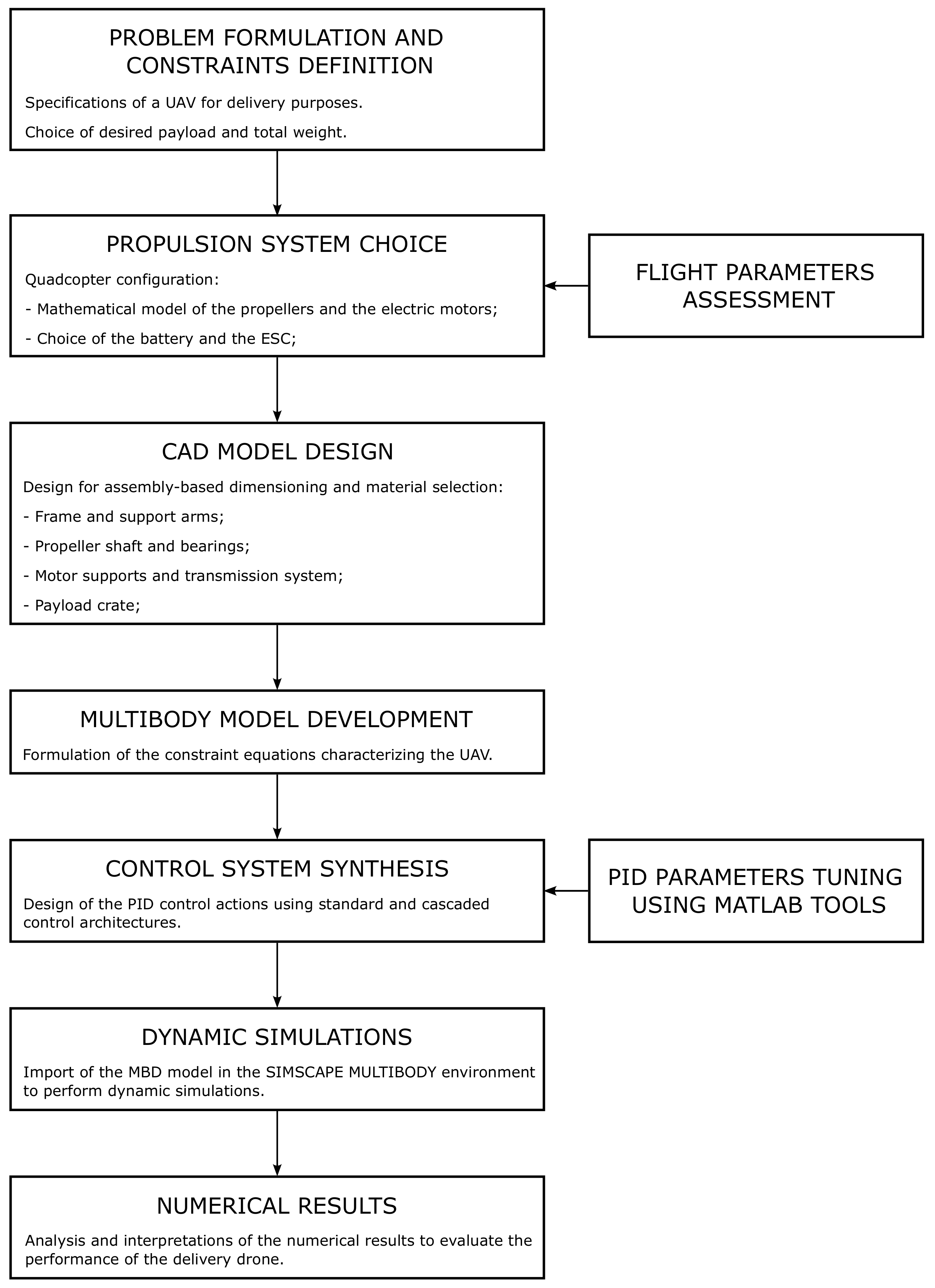
1.1. Formulation of the Problem of Interest for This Investigation
1.2. Literature Review
1.3. Scope and Contributions of This Study
1.4. Organization of the Manuscript
2. Propulsion System Description and Modeling
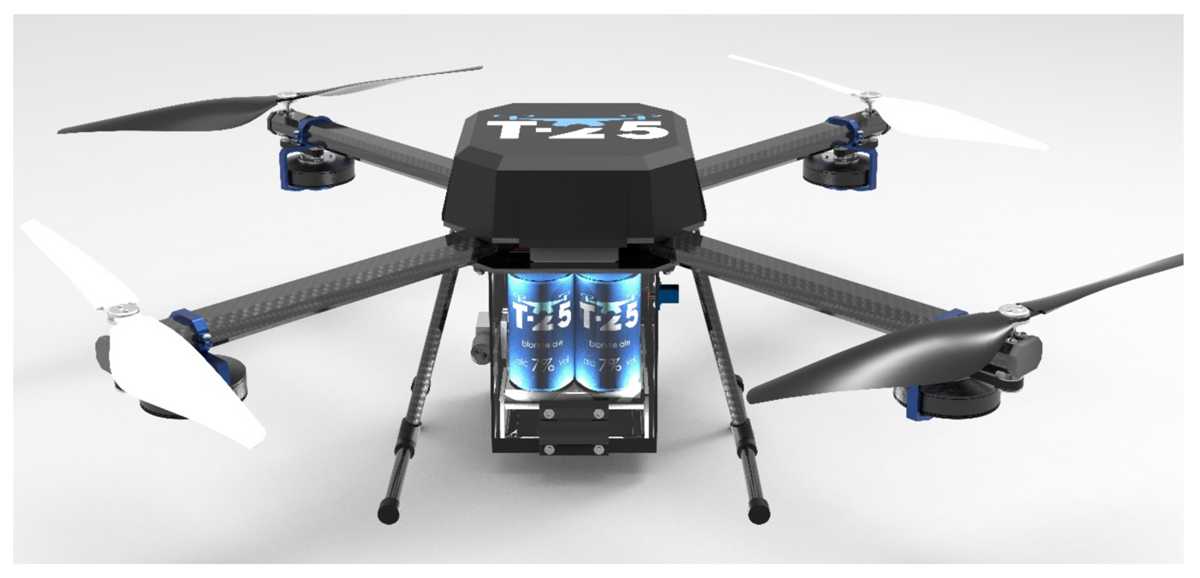
2.1. Main Concept
2.2. Propellers
2.3. Electric Motors
2.4. Batteries
2.5. Electronic Speed Controllers
2.6. Propeller Modeling
2.7. Choices of Motors and Propellers
3. UAV System Computer-Aided Design
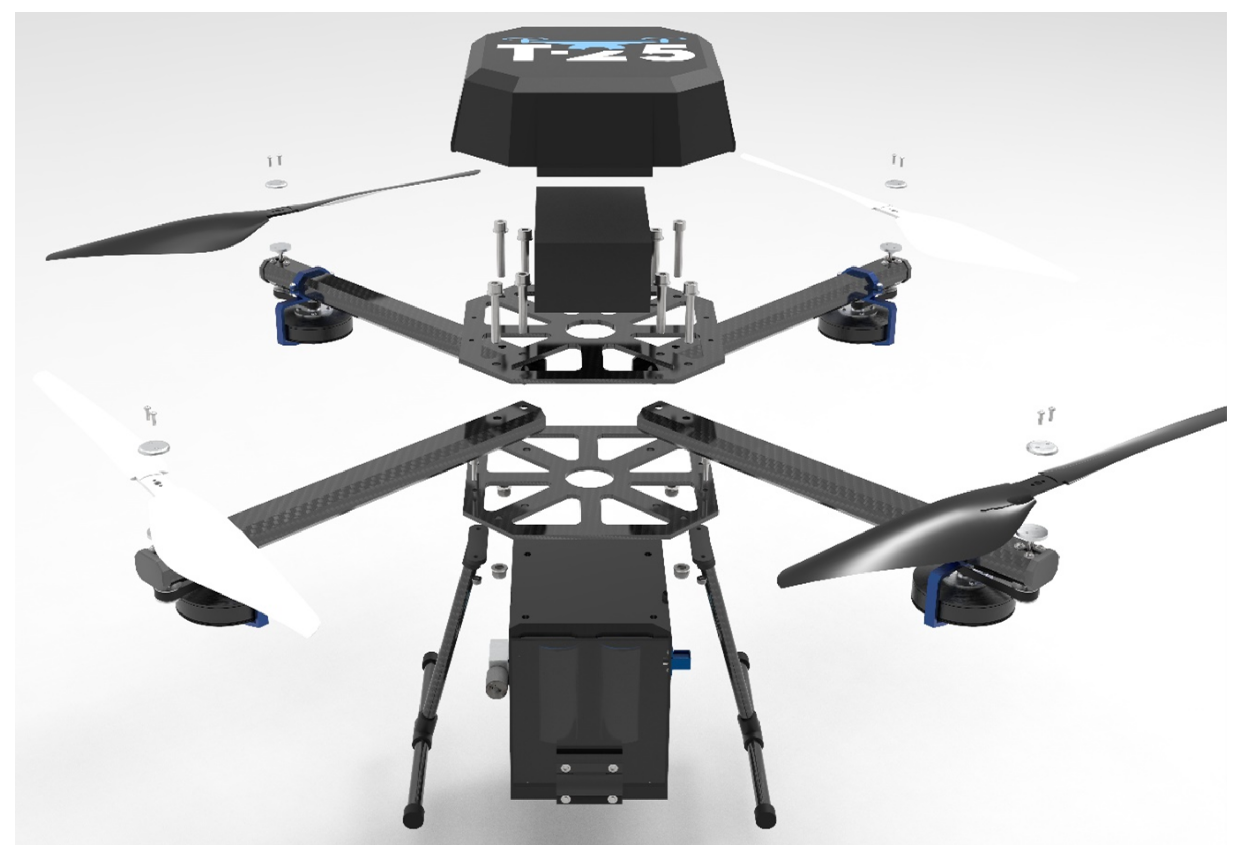
3.1. Complete Geometric Model
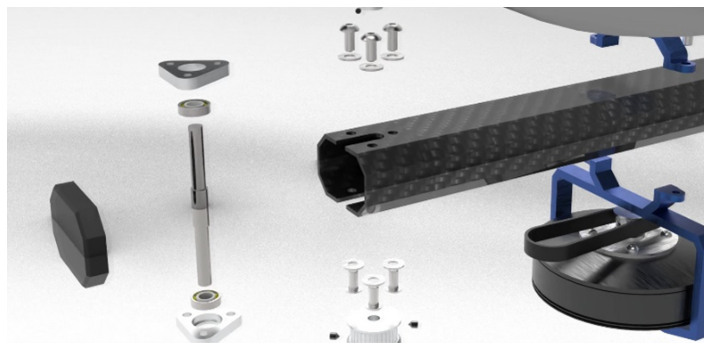
3.2. Support Arms
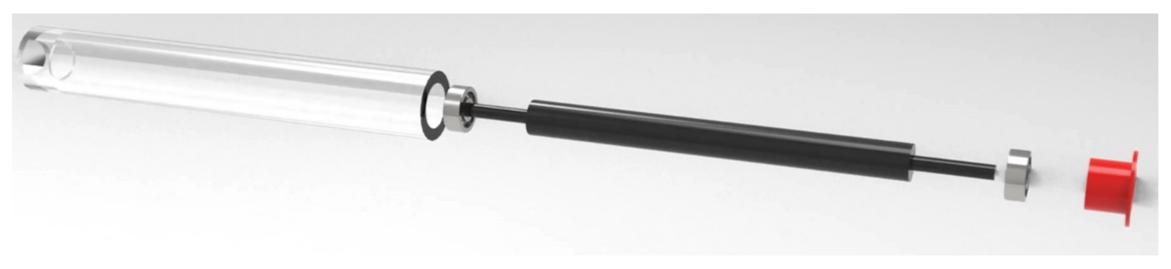
3.3. Propeller Shafts and Bearings
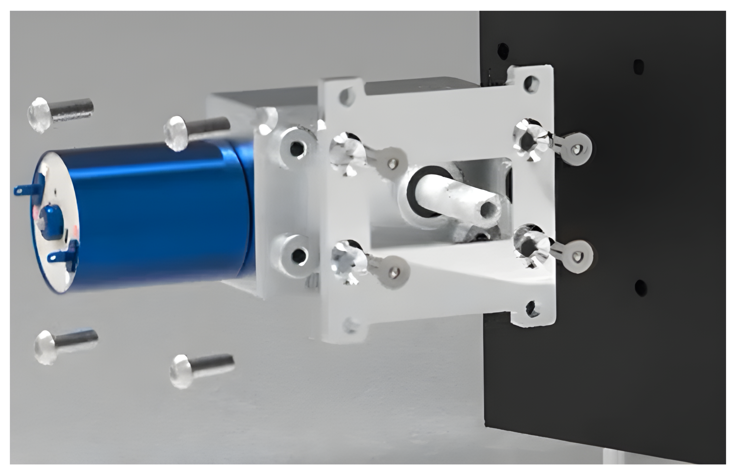
3.4. Motor Supports and Belt Transmissions
3.5. Central Frame
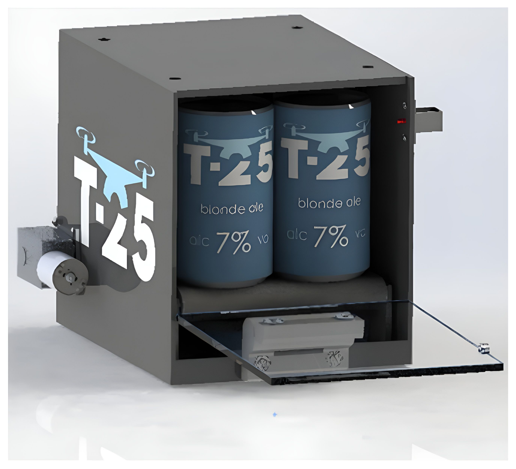
3.6. Beer Crate
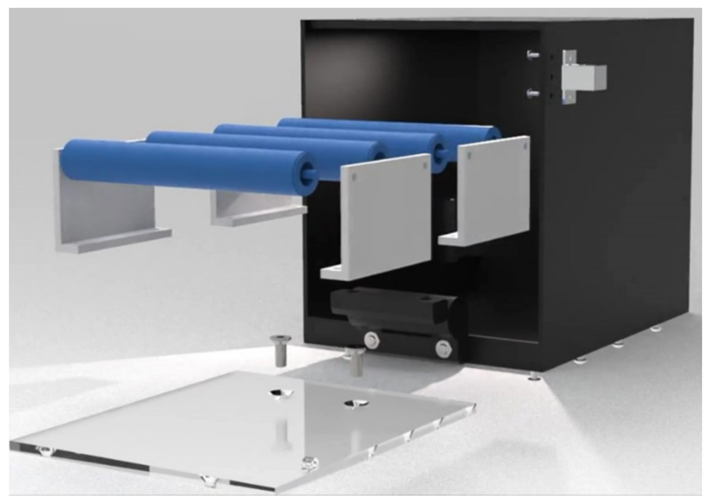
3.7. Rollers, Roller Supports, and Roller Motor
3.8. External Case, Landing Gear, and Battery Cover
4. UAV System Multibody Modeling
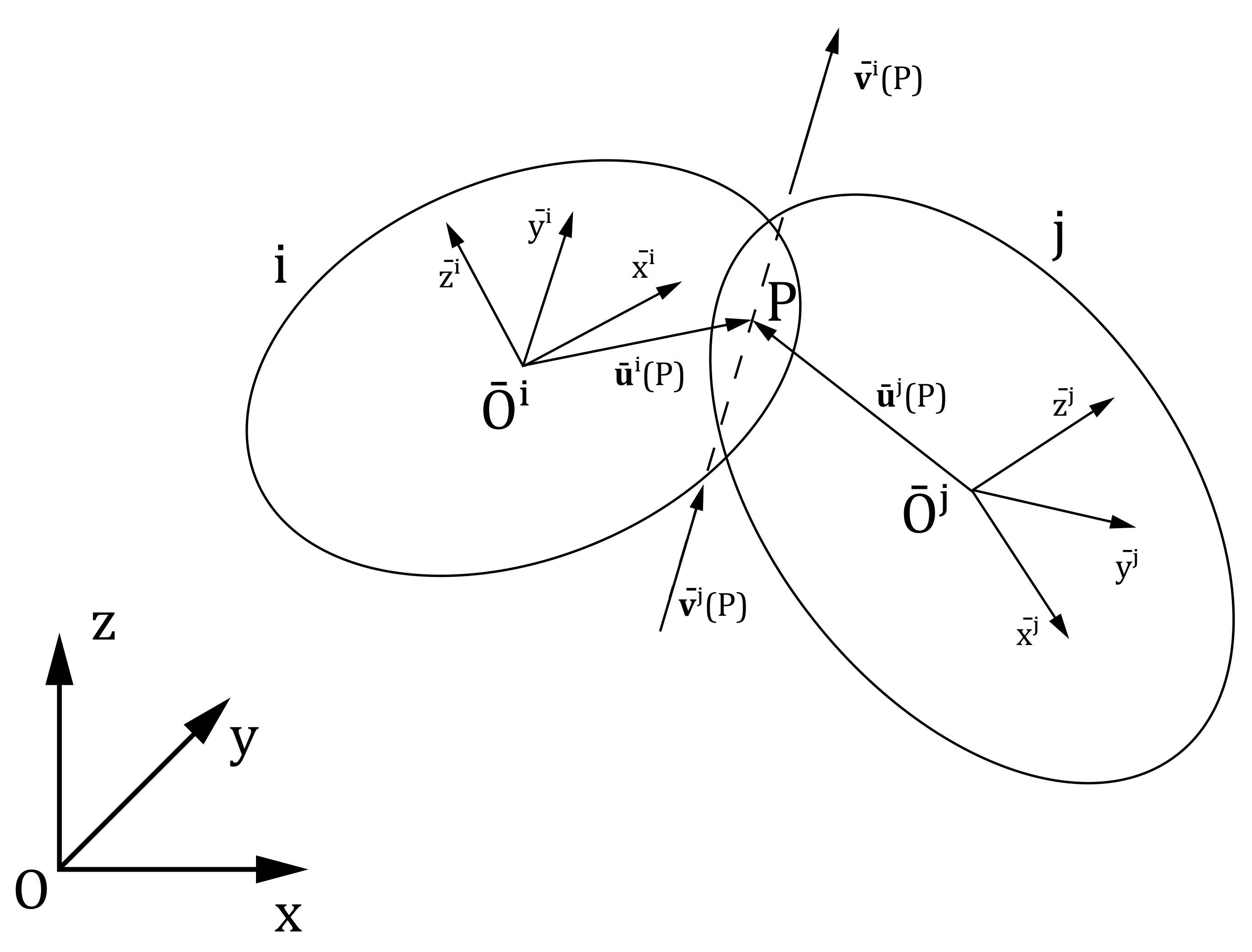
4.1. Mathematical Background
4.2. Kinematic and Dynamic Analysis
- Central frame: body .
- Propeller I: body .
- Propeller II: body .
- Propeller III: body .
- Propeller IV: body .
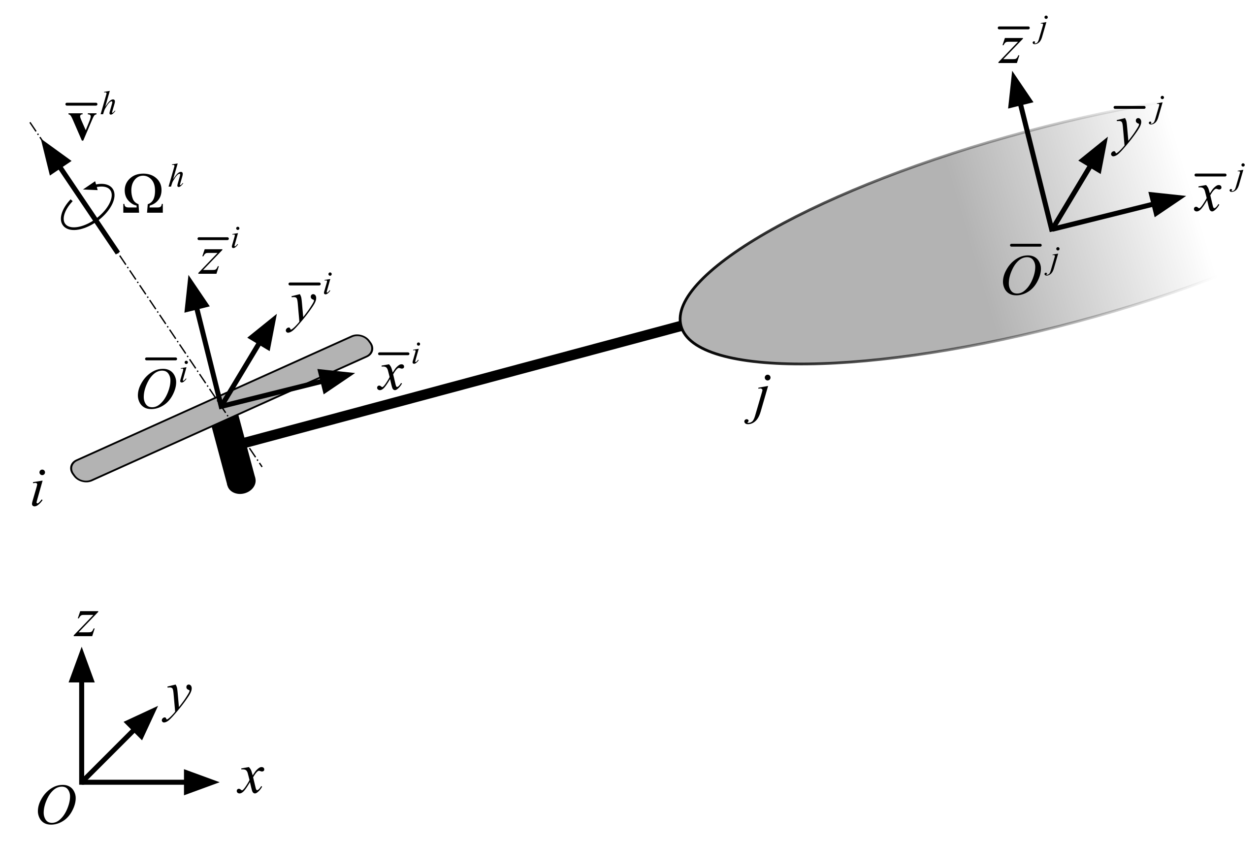
4.3. Mechanical Joints
- Revolute joint I: constraint .
- Revolute joint II: constraint .
- Revolute joint III: constraint .
- Revolute joint IV: constraint .
4.4. Driving Constraints
- Imposed angular velocity I: constraint .
- Imposed angular velocity II: constraint .
- Imposed angular velocity III: constraint .
- Imposed angular velocity IV: constraint .
4.5. External Forces and Control Actions
- Gravitational field: force .
- Wind disturbance: force .
- Contact force I: force .
- Contact force II: force .
- Propeller torque I: .
- Propeller torque II: .
- Propeller torque III: .
- Propeller torque IV: .
4.6. Differential-Algebraic Equations of Motion
4.7. Underactuated Dynamical System
5. UAV System Control Development
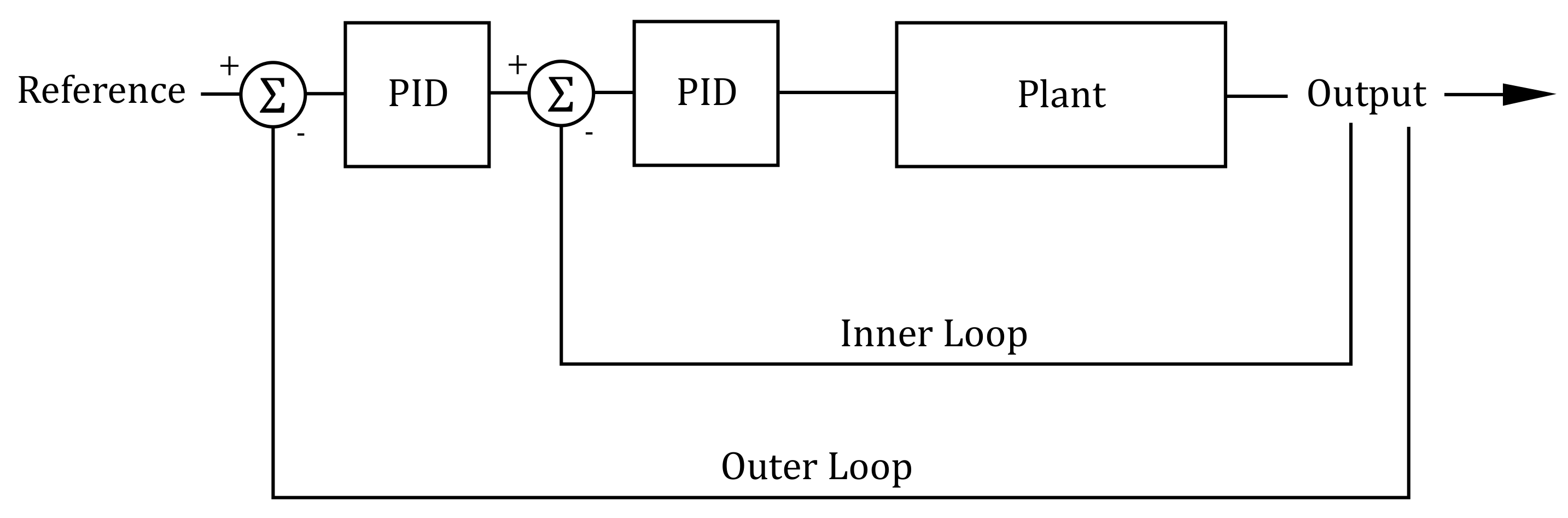
5.1. Control Strategy
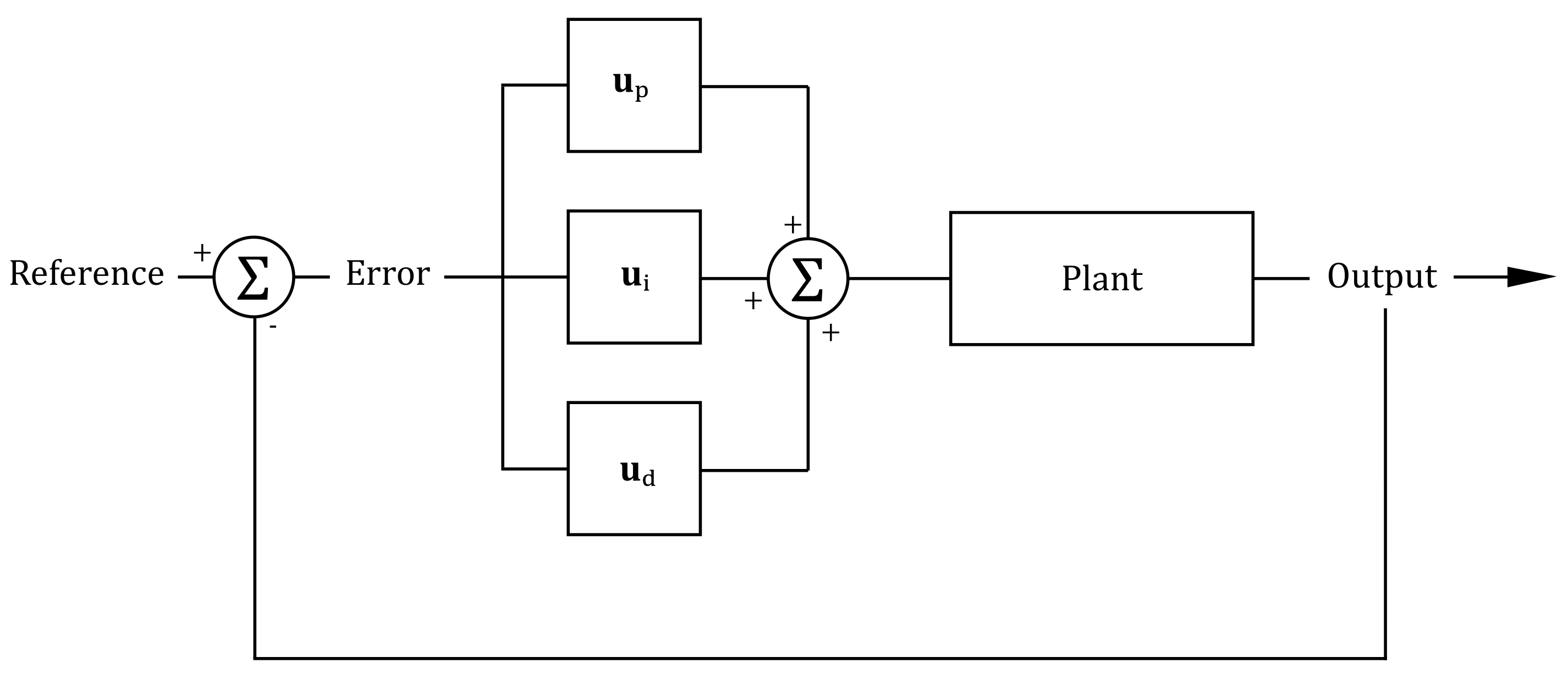
5.2. PID Controller
5.3. UAV System Control
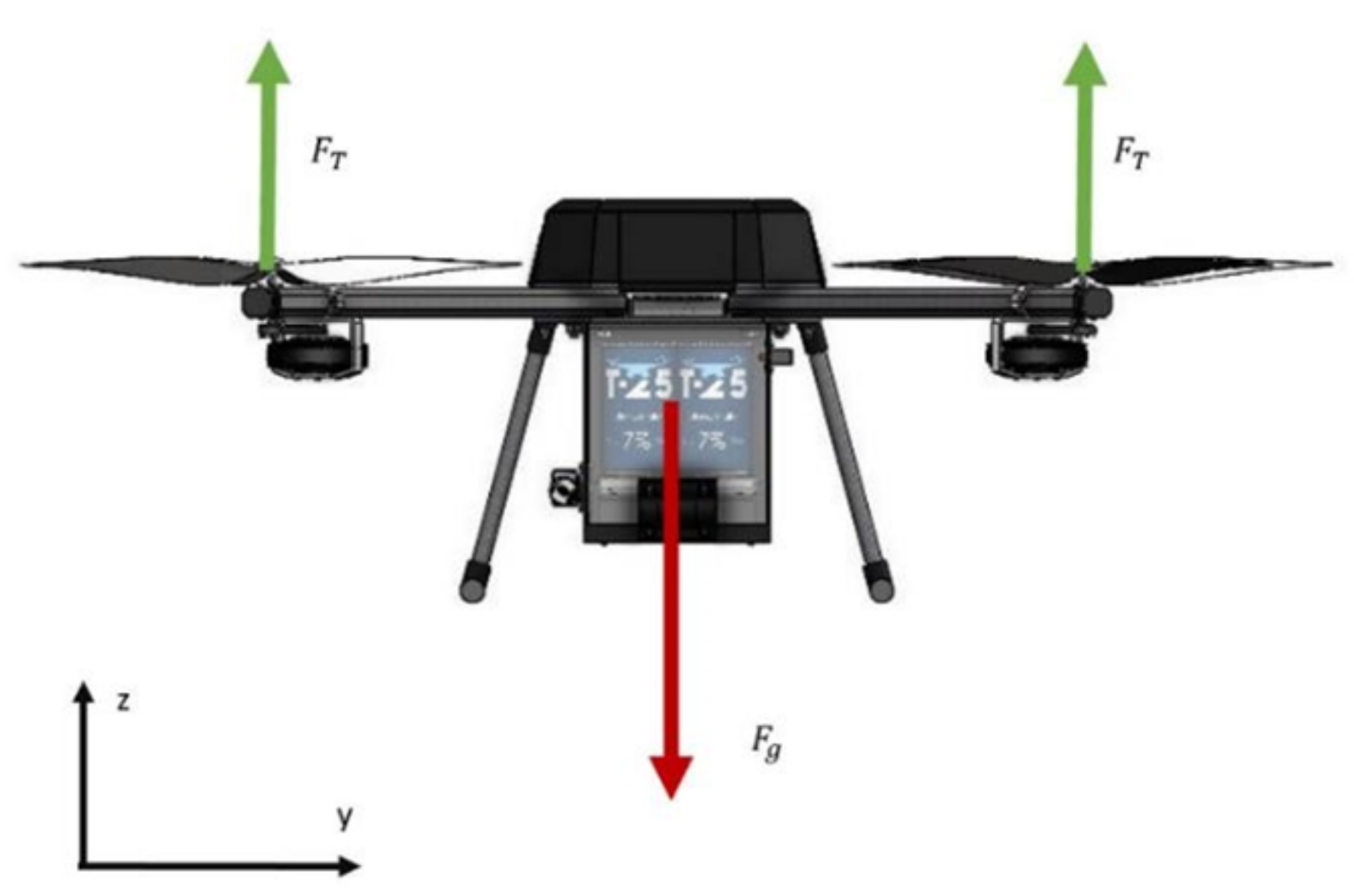
5.3.1. Hovering and Vertical Motion
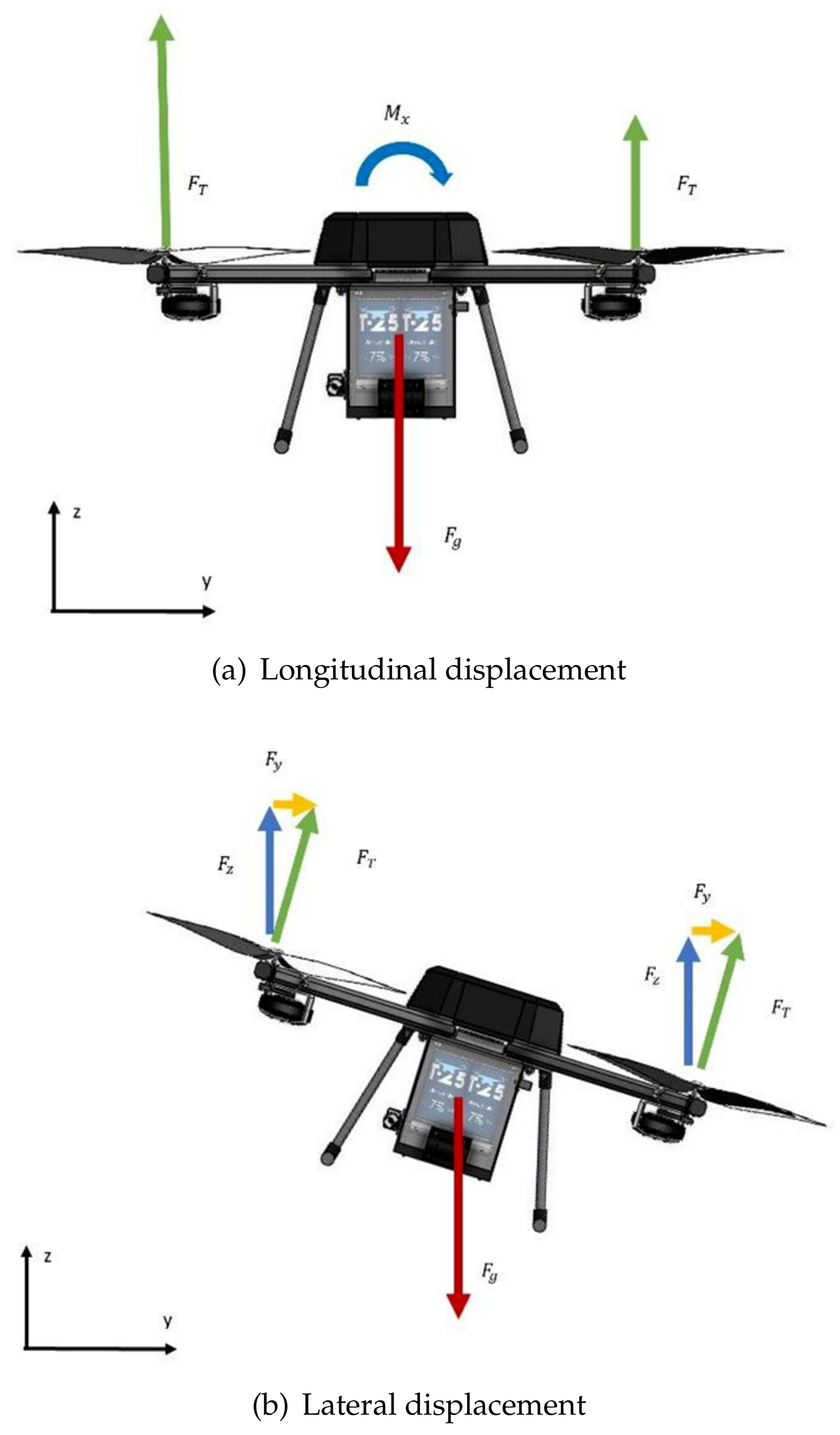
5.3.2. Longitudinal and Lateral Motions
5.3.3. Yaw Motion
5.4. PID Tuner
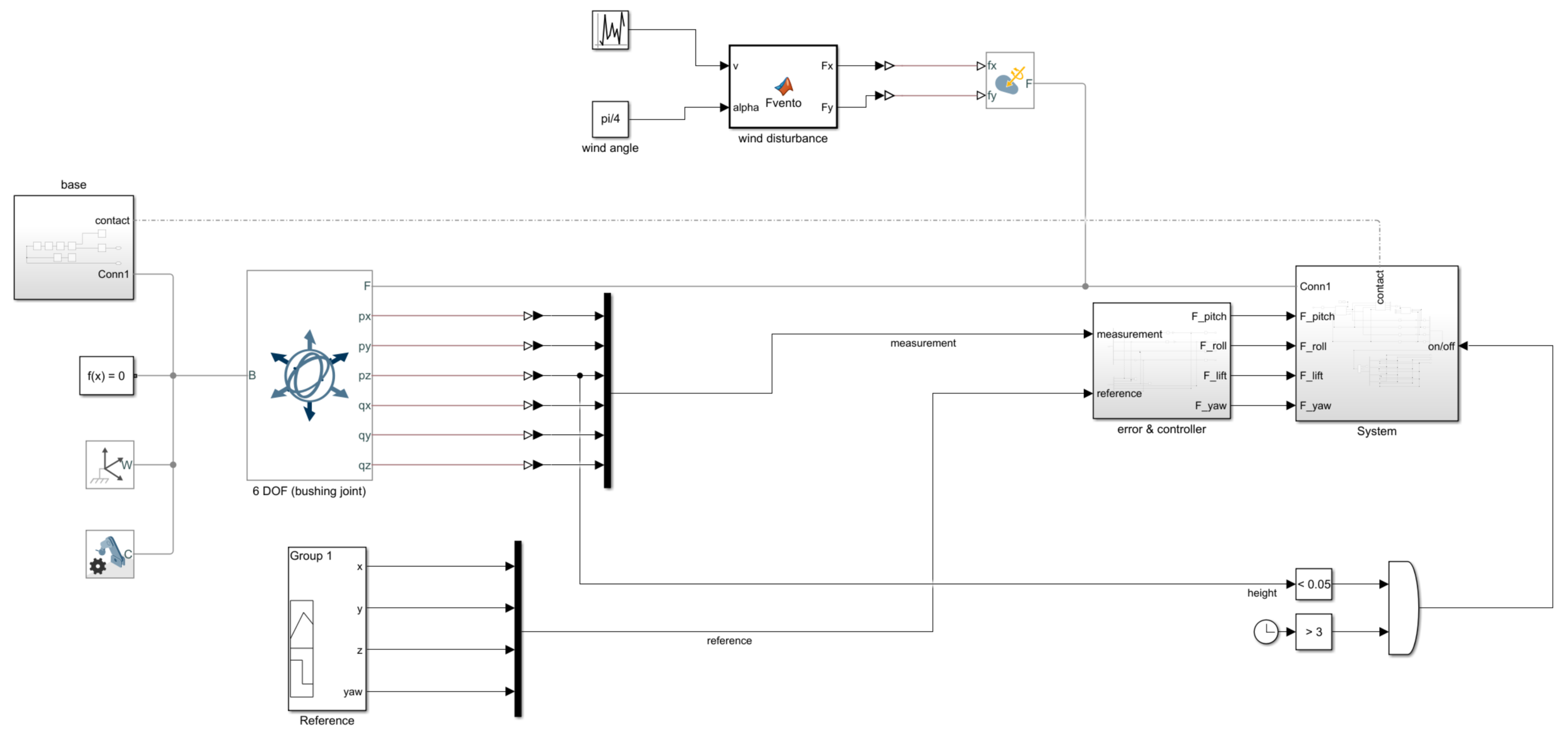
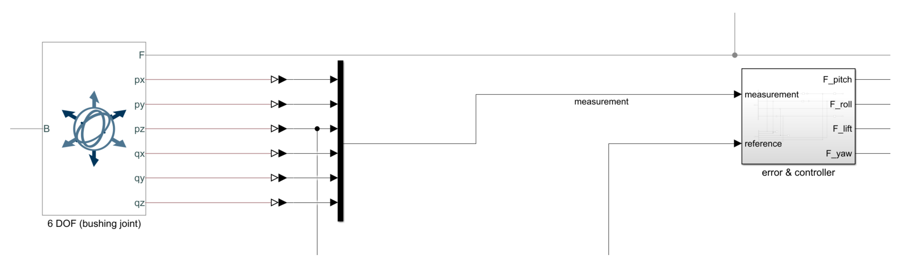
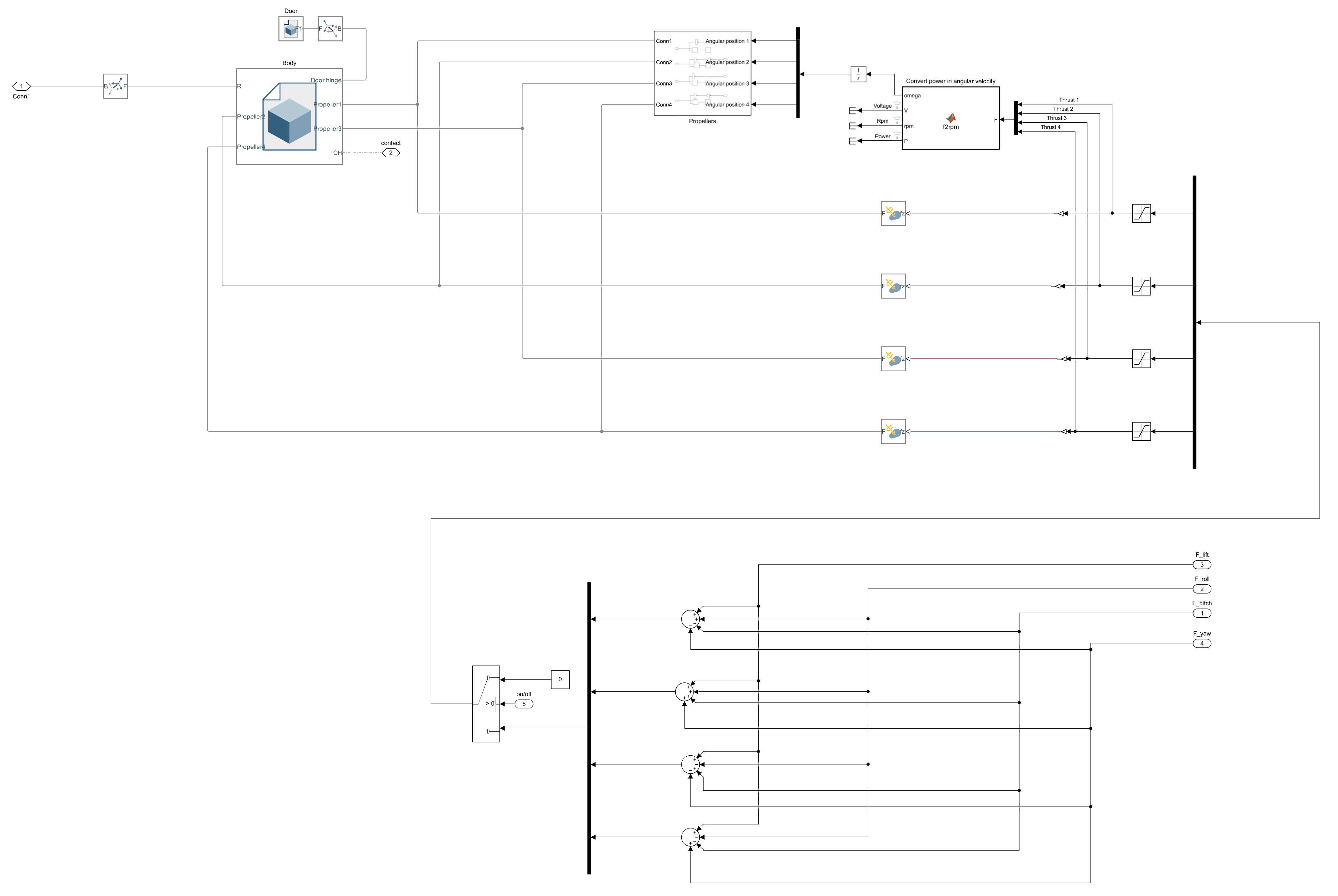
6. SIMSCAPE MULTIBODY Model Description
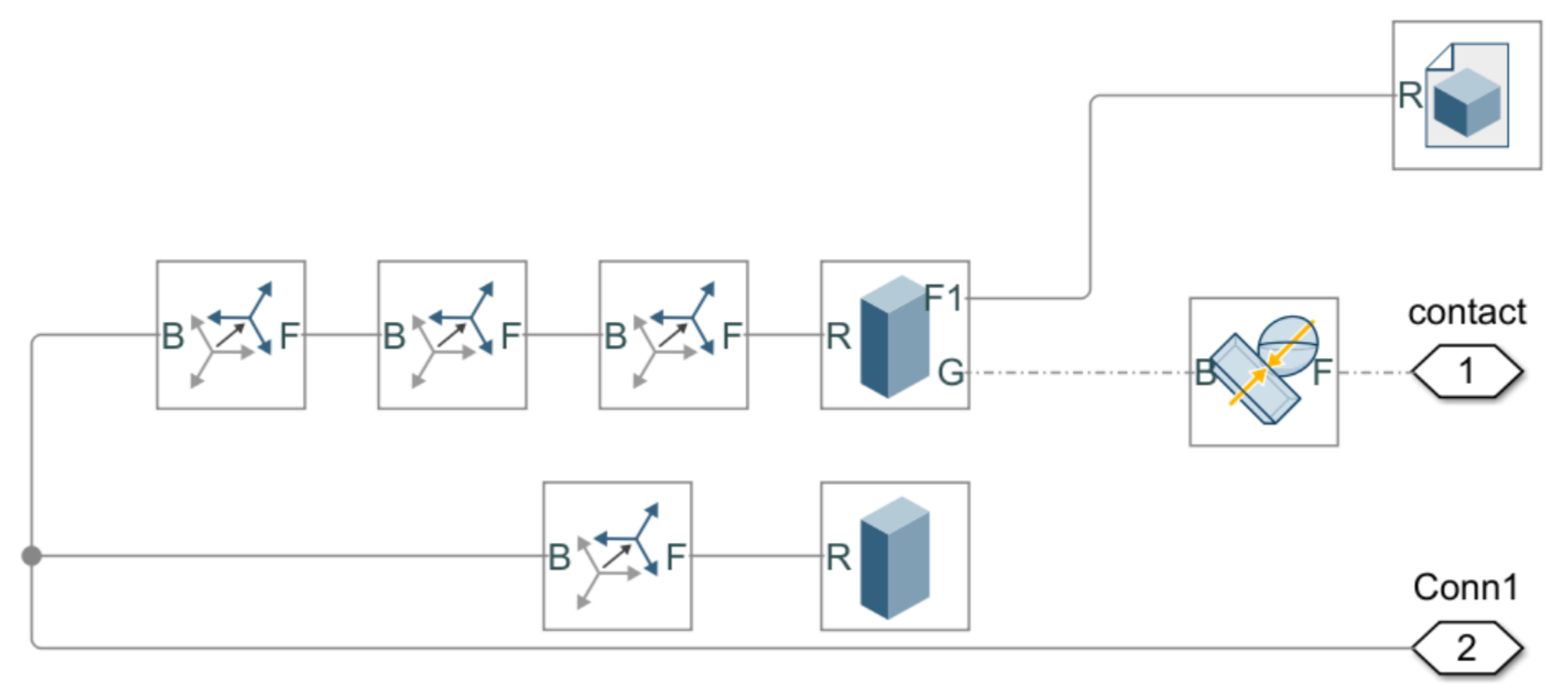
6.1. Computer Model of the Delivery Drone
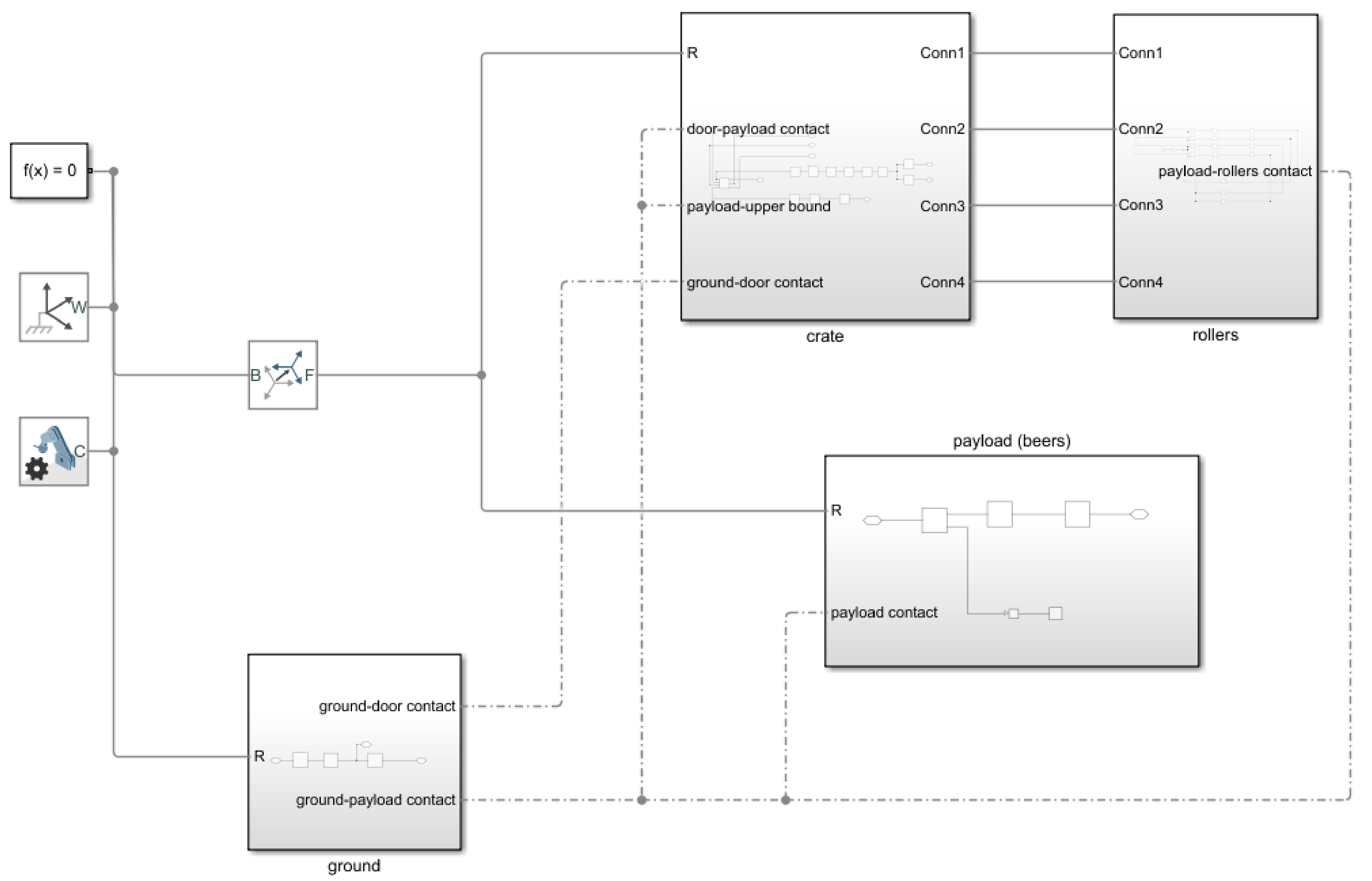
6.2. Computer Model of the Beer Carrier
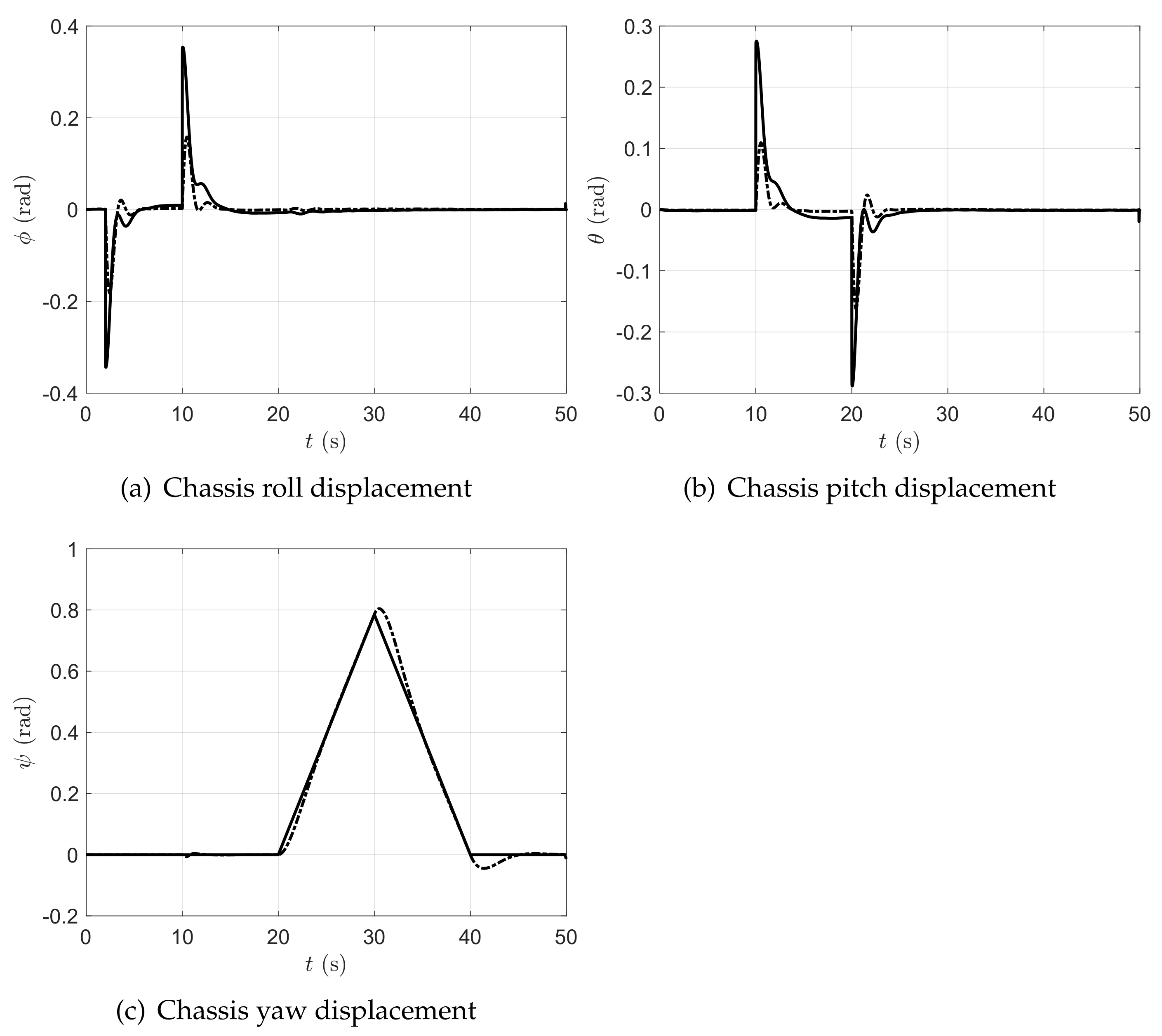
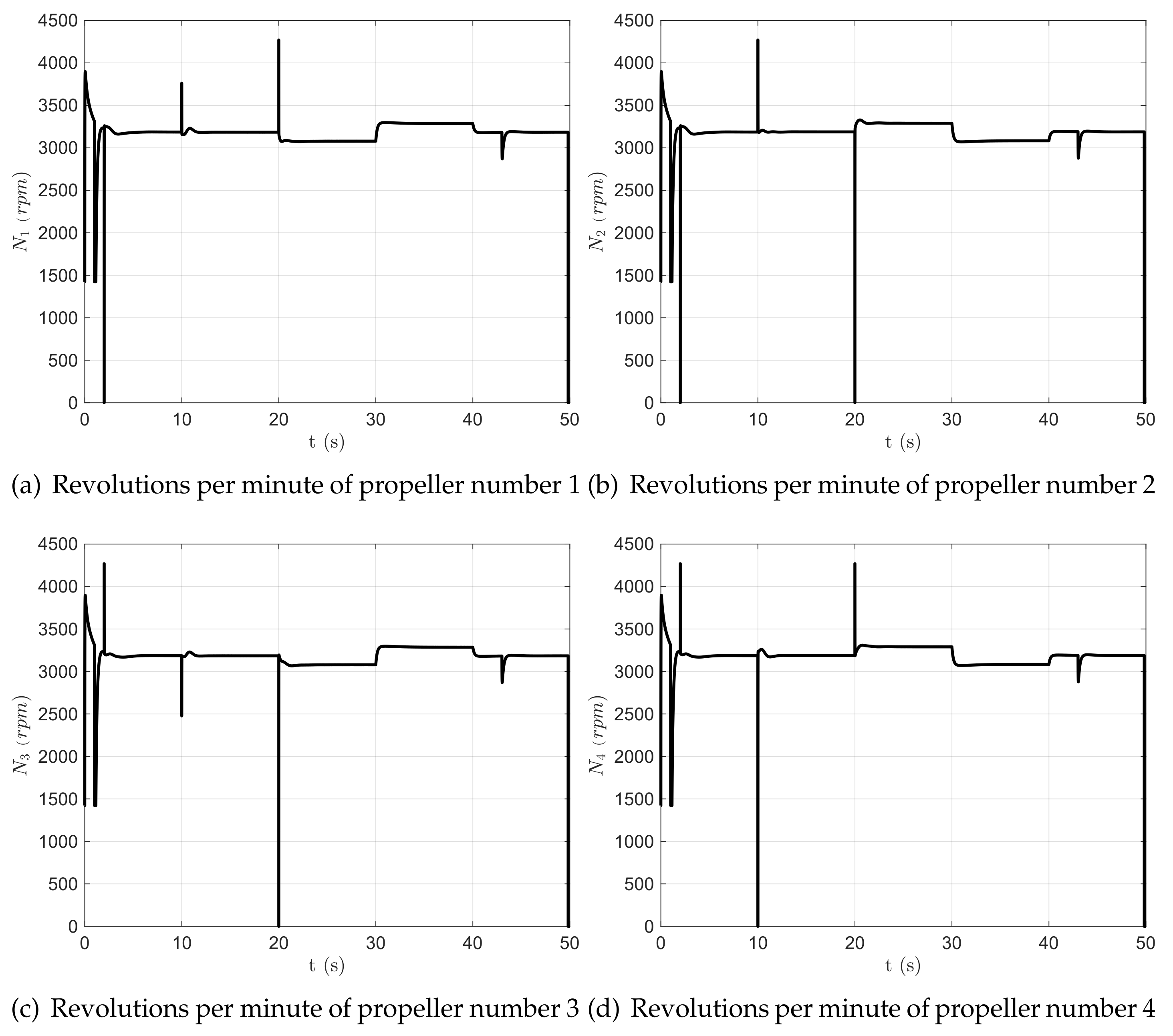
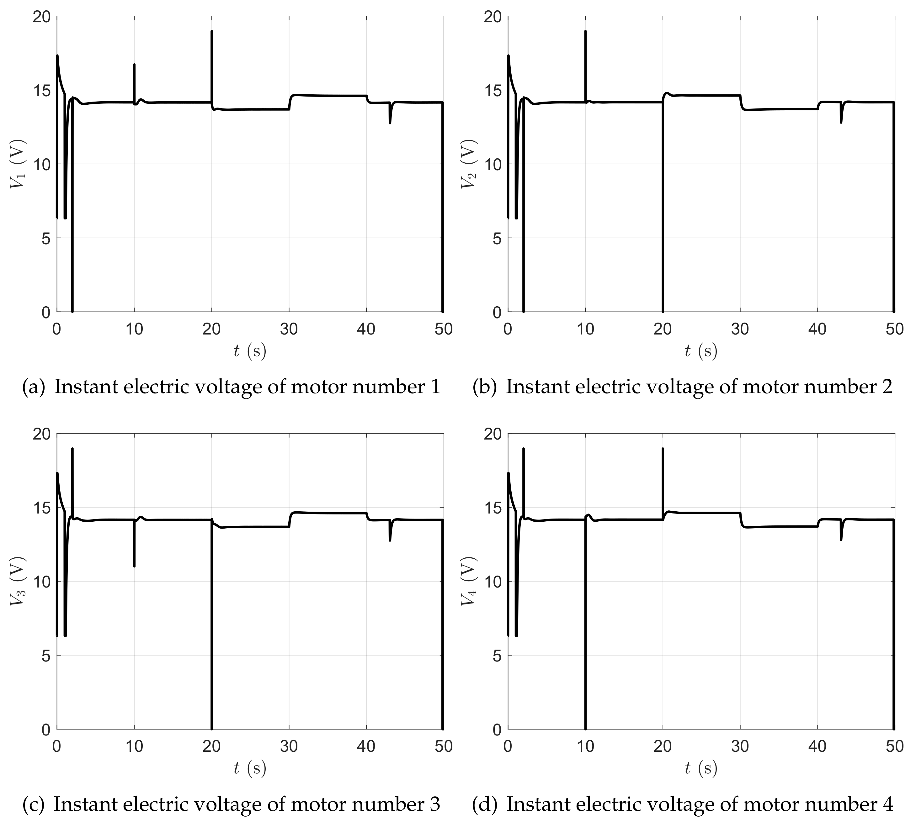
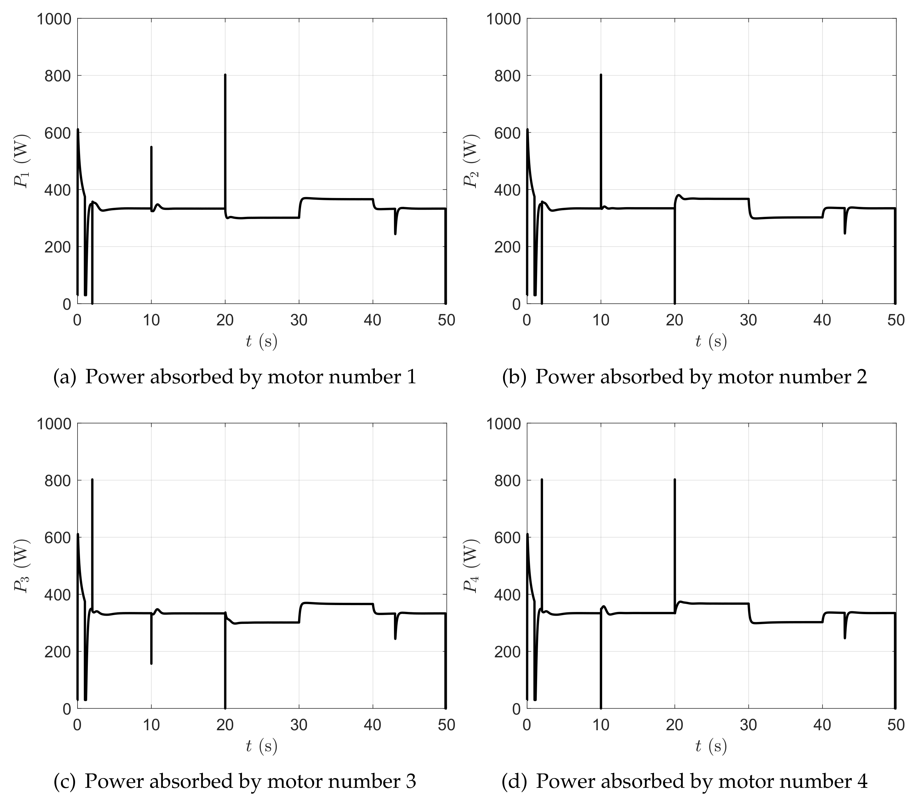
7. Numerical Results and Discussion
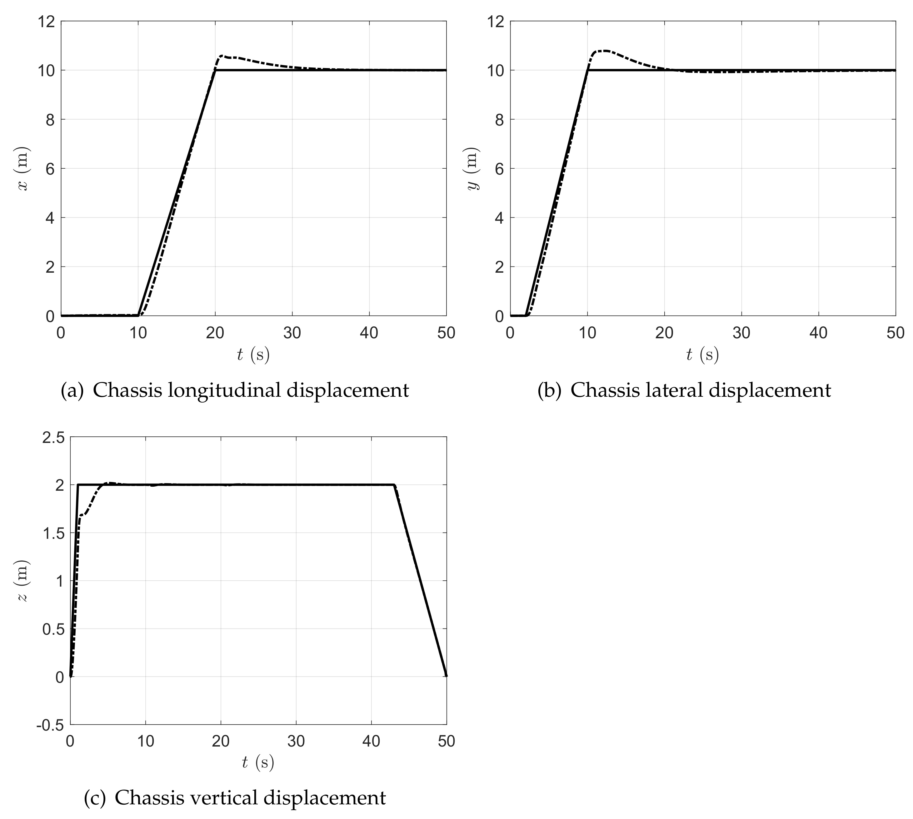
7.1. Presentation of the Numerical Results
7.2. Discussion of the Numerical Results
8. Summary, Conclusions, and Future Developments
Author Contributions
Funding
Data Availability Statement
Conflicts of Interest
References
- Wan, K.; Gao, X.; Hu, Z.; Wu, G. Robust motion control for UAV in dynamic uncertain environments using deep reinforcement learning. Remote Sens. 2020, 12, 640. [Google Scholar] [CrossRef] [Green Version]
- Lopez-Rivera, M.; Cortes-Villada, A.; Giraldo, E. Optimal multivariable control design based on a fuzzy model for an unmanned aerial vehicle. IAENG Int. J. Comput. Sci. 2021, 48, 316–321. [Google Scholar]
- Hu, B.; Wang, J. Deep learning based hand gesture recognition and UAV flight controls. Int. J. Autom. Comput. 2020, 17, 17–29. [Google Scholar] [CrossRef]
- Zhang, Y.; Zhang, Y.; Yu, Z. Path following control for UAV using deep reinforcement learning approach. Guid. Navig. Control 2021, 1, 2150005. [Google Scholar] [CrossRef]
- Shakhatreh, H.; Sawalmeh, A.H.; Al-Fuqaha, A.; Dou, Z.; Almaita, E.; Khalil, I.; Othman, N.S.; Khreishah, A.; Guizani, M. Unmanned aerial vehicles (UAVs): A survey on civil applications and key research challenges. IEEE Access 2019, 7, 48572–48634. [Google Scholar] [CrossRef]
- Azam, M.A.; Mittelmann, H.D.; Ragi, S. UAV formation shape control via decentralized markov decision processes. Algorithms 2021, 14, 91. [Google Scholar] [CrossRef]
- Bai, D.; Tian, J.; Li, D.; Li, S. Multiple UAVs Tracking for Moving Ground Target. Eng. Lett. 2022, 30, 829–834. [Google Scholar]
- Belmonte, L.M.; Morales, R.; Fernández-Caballero, A. Computer vision in autonomous unmanned aerial vehicles—A systematic mapping study. Appl. Sci. 2019, 9, 3196. [Google Scholar] [CrossRef] [Green Version]
- Hu, J.; Zhang, H.; Li, Z.; Zhao, C.; Xu, Z.; Pan, Q. Object traversing by monocular UAV in outdoor environment. Asian J. Control 2021, 23, 2766–2775. [Google Scholar] [CrossRef]
- Cifuentes-Molano, M.F.; Hernandez, B.S.; Giraldo, E. Comparison of Different Control Techniques on a Bipedal Robot of 6 Degrees of Freedom. IAENG Int. J. Appl. Math. 2021, 51, 1–7. [Google Scholar]
- Gu, S.; Chen, J.; Tian, Q. An implicit asynchronous variational integrator for flexible multibody dynamics. Comput. Methods Appl. Mech. Eng. 2022, 401, 115660. [Google Scholar] [CrossRef]
- Wang, K.; Tian, Q. A nonsmooth method for spatial frictional contact dynamics of flexible multibody systems with large deformation. Int. J. Numer. Methods Eng. 2023, 124, 752–779. [Google Scholar] [CrossRef]
- Shabana, A.A. Integration of computer-aided design and analysis: Application to multibody vehicle systems. Int. J. Veh. Perform. 2019, 5, 300–327. [Google Scholar] [CrossRef]
- Citarella, R.; Armentani, E.; Caputo, F.; Naddeo, A. FEM and BEM analysis of a human mandible with added temporomandibular joints. Open Mech. Eng. J. 2012, 6, 100–114. [Google Scholar] [CrossRef] [Green Version]
- Cappetti, N.; Naddeo, A.; Naddeo, F.; Solitro, G. Finite elements/Taguchi method based procedure for the identification of the geometrical parameters significantly affecting the biomechanical behavior of a lumbar disc. Comput. Methods Biomech. Biomed. Eng. 2016, 19, 1278–1285. [Google Scholar] [CrossRef] [PubMed]
- Muscat, M.; Cammarata, A.; Maddio, P.D.; Sinatra, R. Design and development of a towfish to monitor marine pollution. Euro-Mediterr. J. Environ. Integr. 2018, 3, 1–12. [Google Scholar] [CrossRef]
- Tanev, T.; Cammarata, A.; Marano, D.; Sinatra, R. Elastostatic model of a new hybrid minimally-invasive-surgery robot. In Proceedings of the 14th IFToMM World Congress, Taipei, Taiwan, 25–30 October 2015. [Google Scholar]
- De Simone, M.C.; Celenta, G.; Rivera, Z.B.; Guida, D. Mechanism Design for a Low-Cost Automatic Breathing Applications for Developing Countries. In Proceedings of the International Conference “New Technologies, Development and Applications”, Sarajevo, Bosnia and Herzegovina, 23–25 June 2022; pp. 345–352. [Google Scholar]
- Mangoni, D.; Soldati, A. Model-based simulation of dynamic behaviour of electric powertrains and their limitation induced by battery current saturation. Int. J. Veh. Perform. 2021, 7, 156–169. [Google Scholar] [CrossRef]
- Cammarata, A.; Lacagnina, M.; Sinatra, R. Closed-form solutions for the inverse kinematics of the Agile Eye with constraint errors on the revolute joint axes. In Proceedings of the 2016 IEEE/RSJ International Conference on Intelligent Robots and Systems (IROS), Daejeon, Republic of Korea, 9–14 October 2016; pp. 317–322. [Google Scholar]
- Tasora, A.; Mangoni, D.; Benatti, S.; Garziera, R. Solving variational inequalities and cone complementarity problems in nonsmooth dynamics using the alternating direction method of multipliers. Int. J. Numer. Methods Eng. 2021, 122, 4093–4113. [Google Scholar] [CrossRef]
- Huang, Z.; Xi, F.; Huang, T.; Dai, J.S.; Sinatra, R. Lower-mobility parallel robots: Theory and applications. Adv. Mech. Eng. 2010, 2, 927930. [Google Scholar] [CrossRef] [Green Version]
- Cammarata, A.; Sinatra, R.; Rigano, A.; Lombardo, M.; Maddio, P.D. Design of a large deployable reflector opening system. Machines 2020, 8, 7. [Google Scholar] [CrossRef] [Green Version]
- Kant, R.; Nigam, V.K.; Kumar, R. Design and Analysis of Unmanned Aerial Vehicle (Uav) Using Solidworks 2016 Edition. Int. Res. J. Eng. Technol 2019, 6, 5132–5138. [Google Scholar]
- Ballous, K.A.; Khalifa, A.N.; Abdulwadood, A.; Al-Shabi, M.; Assad, M.E.H. Medical kit: Emergency drone. In Proceedings of the Unmanned Systems Technology XXII. International Society for Optics and Photonics, Online Only, 27 April–9 May 2020; Volume 11425, p. 114250V. [Google Scholar]
- Zhafri, Z.; Effendi, M.; Rosli, M.F. Optimization of assembly process and environmental impact using DFMA and sustainable design analysis: Case study of drone. Aip Conf. Proc. 2018, 2030, 020074. [Google Scholar]
- Meenakshipriya, B.; Raja, N.B.; Faroshkhan, S.; Matris, S. Design and fabrication of 3D printed QuadDrone for altitude measurement. Int. J. Aerosp. Syst. Sci. Eng. 2021, 1, 85–94. [Google Scholar] [CrossRef]
- Benito, J.A.; Glez-de Rivera, G.; Garrido, J.; Ponticelli, R. Design considerations of a small UAV platform carrying medium payloads. In Proceedings of the Design of Circuits and Integrated Systems, Madrid, Spain, 26–28 November 2014; pp. 1–6. [Google Scholar]
- Tnunay, H.; Abdurrohman, M.Q.; Nugroho, Y.; Inovan, R.; Cahyadi, A.; Yamamoto, Y. Auto-tuning quadcopter using Loop Shaping. In Proceedings of the 2013 International Conference on Computer, Control, Informatics and Its Applications (IC3INA), Jakarta, Indonesia, 19–21 November 2013; pp. 111–115. [Google Scholar]
- De Simone, M.C.; Russo, S.; Rivera, Z.B.; Guida, D. Multibody model of a UAV in presence of wind fields. In Proceedings of the 2017 International Conference on Control, Artificial Intelligence, Robotics & Optimization (ICCAIRO), Prague, Czech Republic, 20–22 May 2017; pp. 83–88. [Google Scholar]
- Hai-long, F.Q.d.P. The application of cascade PID control in UAV attitude control. Microcomput. Inf. 2009, 25, 9–10. [Google Scholar]
- Amir, M.Y.; Abbass, V. Modeling of quadrotor helicopter dynamics. In Proceedings of the 2008 International Conference on Smart Manufacturing Application, Goyangi, Republic of Korea, 9–11 April 2008; pp. 100–105. [Google Scholar]
- Razinkova, A.; Gaponov, I.; Cho, H.C. Adaptive control over quadcopter UAV under disturbances. In Proceedings of the 2014 14th International Conference on Control, Automation and Systems (ICCAS 2014), Gyeonggi-do, Republic of Korea, 22–25 October 2014; pp. 386–390. [Google Scholar]
- Fernando, H.; De Silva, A.; De Zoysa, M.; Dilshan, K.; Munasinghe, S. Modelling, simulation and implementation of a quadrotor UAV. In Proceedings of the 2013 IEEE 8th International Conference on Industrial and Information Systems, Peradeniya, Sri Lanka, 17–20 December 2013; pp. 207–212. [Google Scholar]
- Pessen, D.W. A new look at PID-controller tuning. J. Dyn. Sys. Meas. Control 1994, 116, 553–557. [Google Scholar] [CrossRef]
- Azeemi, N.Z. Cooperative Trajectory and Launch Power Optimization of UAV Deployed in Cross-Platform Battlefields. Int. Assoc. Eng. Eng. Lett. 2021, 29, 57–68. [Google Scholar]
- De Simone, M.C.; Guida, D. Control design for an under-actuated UAV model. FME Trans. 2018, 46, 443–452. [Google Scholar]
- Du, H.; Wang, W.; Xu, C.; Xiao, R.; Sun, C. Real-time onboard 3D state estimation of an unmanned aerial vehicle in multi-environments using multi-sensor data fusion. Sensors 2020, 20, 919. [Google Scholar] [CrossRef] [PubMed] [Green Version]
- Malgaca, L.; Lök, Ş.İ. Measurement and modeling of a flexible manipulator for vibration control using five-segment S-curve motion. Trans. Inst. Meas. Control 2022, 44, 1545–1556. [Google Scholar] [CrossRef]
- Guo, A.; Zhou, Z.; Zhu, X.; Bai, F. Low-cost sensors state estimation algorithm for a small hand-launched Solar-powered UAV. Sensors 2019, 19, 4627. [Google Scholar] [CrossRef] [PubMed] [Green Version]
- Pan, Y.; Dai, W.; Xiong, Y.; Xiang, S.; Mikkola, A. Tree-topology-oriented modeling for the real-time simulation of sedan vehicle dynamics using independent coordinates and the rod-removal technique. Mech. Mach. Theory 2020, 143, 103626. [Google Scholar] [CrossRef]
- Villecco, F.; Pellegrino, A. Entropic measure of epistemic uncertainties in multibody system models by axiomatic design. Entropy 2017, 19, 291. [Google Scholar] [CrossRef] [Green Version]
- Villecco, F. On the evaluation of errors in the virtual design of mechanical systems. Machines 2018, 6, 36. [Google Scholar] [CrossRef] [Green Version]
- De Simone, M.C.; Veneziano, S.; Guida, D. Design of a Non-Back-Drivable Screw Jack Mechanism for the Hitch Lifting Arms of Electric-Powered Tractors. Actuators 2022, 11, 358. [Google Scholar] [CrossRef]
- Kaiser, I.; Strano, S.; Terzo, M.; Tordela, C. Anti-yaw damping monitoring of railway secondary suspension through a nonlinear constrained approach integrated with a randomly variable wheel-rail interaction. Mech. Syst. Signal Process. 2021, 146, 107040. [Google Scholar] [CrossRef]
- Bettega, J.; Richiedei, D. Trajectory tracking in an underactuated, non-minimum phase two-link multibody system through model predictive control with embedded reference dynamics. Mech. Mach. Theory 2023, 180, 105165. [Google Scholar] [CrossRef]
- Kaiser, I.; Strano, S.; Terzo, M.; Tordela, C. Estimation of the railway equivalent conicity under different contact adhesion levels and with no wheelset sensorization. Veh. Syst. Dyn. 2023, 61, 19–37. [Google Scholar] [CrossRef]
- Quan, Q. Introduction to Multicopter Design and Control; Springer: Berlin/Heidelberg, Germany, 2017; pp. 150–160. [Google Scholar]
- Torenbeek, E.; Wittenberg, H. Flight Physics: Essentials of Aeronautical Disciplines and Technology, with Historical Notes; Springer Science & Business Media: Berlin/Heidelberg, Germany, 2009. [Google Scholar]
- Quan, Q.; Dai, X.; Wang, S. Multicopter Design and Control Practice: A Series Experiments Based on MATLAB and Pixhawk; Springer Nature: Berlin/Heidelberg, Germany, 2020. [Google Scholar]
- Hassani, H.; Mansouri, A.; Ahaitouf, A. Mechanical modeling, control and simulation of a quadrotor UAV. In Proceedings of the International Conference on Electronic Engineering and Renewable Energy, Saidia, Morocco, 13–15 April 2020; pp. 441–449. [Google Scholar]
- Ononiwu, G.; Onojo, O.; Ozioko, O.; Nosiri, O. Quadcopter design for payload delivery. J. Comput. Commun. 2016, 4, 1–12. [Google Scholar] [CrossRef] [Green Version]
- Patel, K.; Barve, J. Modeling, simulation and control study for the quad-copter UAV. In Proceedings of the 2014 9th International Conference on Industrial and Information Systems (ICIIS), Gwalior, India, 15–17 December 2014; pp. 1–6. [Google Scholar]
- Luukkonen, T. Modelling and control of quadcopter. Indep. Res. Proj. Appl. Math. Espoo 2011, 22, 22. [Google Scholar]
- Bai, Q.; Shehata, M.; Nada, A. Review study of using Euler angles and Euler parameters in multibody modeling of spatial holonomic and non-holonomic systems. Int. J. Dyn. Control 2022, 10, 1707–1725. [Google Scholar] [CrossRef]
- Pappalardo, C.M.; Guida, D. On the Lagrange multipliers of the intrinsic constraint equations of rigid multibody mechanical systems. Arch. Appl. Mech. 2018, 88, 419–451. [Google Scholar] [CrossRef]
- Guida, R.; De Simone, M.; Dašić, P.; Guida, D. Modeling techniques for kinematic analysis of a six-axis robotic arm. In Proceedings of the IOP Conference Series: Materials Science and Engineering, Oradea, Romania, 30–31 May 2019; Volume 568, p. 012115. [Google Scholar]
- Yilmaz, Z.; Yilmaz, O.; Bingul, Z. Design, analysis and simulation of a 6-DOF serial manipulator. Kocaeli J. Sci. Eng. 2020, 3, 9–15. [Google Scholar] [CrossRef]
- Shabana, A.A. Dynamics of Multibody Systems; Cambridge University Press: Cambridge, UK, 2003. [Google Scholar]
- Shabana, A.A. Computational Dynamics; John Wiley & Sons: Hoboken, NJ, USA, 2009. [Google Scholar]
- Pappalardo, C.M.; Guida, D. A comparative study of the principal methods for the analytical formulation and the numerical solution of the equations of motion of rigid multibody systems. Arch. Appl. Mech. 2018, 88, 2153–2177. [Google Scholar] [CrossRef]
- Blajer, W. Methods for constraint violation suppression in the numerical simulation of constrained multibody systems–A comparative study. Comput. Methods Appl. Mech. Eng. 2011, 200, 1568–1576. [Google Scholar] [CrossRef]
- Flores, P.; Machado, M.; Seabra, E.; Tavares da Silva, M. A parametric study on the Baumgarte stabilization method for forward dynamics of constrained multibody systems. J. Comput. Nonlinear Dyn. 2011, 6, 011019. [Google Scholar] [CrossRef]
- Pappalardo, C.M.; Guida, D. Dynamic analysis of planar rigid multibody systems modeled using natural absolute coordinates. Appl. Comput. Mech. 2018, 12, 73–110. [Google Scholar] [CrossRef]
- Marques, F.; Souto, A.P.; Flores, P. On the constraints violation in forward dynamics of multibody systems. Multibody Syst. Dyn. 2017, 39, 385–419. [Google Scholar] [CrossRef] [Green Version]
- Flores, P.; Nikravesh, P.E. Comparison of different methods to control constraints violation in forward multibody dynamics. In Proceedings of the International Design Engineering Technical Conferences and Computers and Information in Engineering Conference, Portland, OR, USA, 4–7 August 2013; Volume 55966, p. V07AT10A028. [Google Scholar]
- Seifried, R. Dynamics of Underactuated Multibody Systems; Springer: Berlin/Heidelberg, Germany, 2014. [Google Scholar]
- Guida, D.; Pappalardo, C.M. Forward and inverse dynamics of nonholonomic mechanical systems. Meccanica 2014, 49, 1547–1559. [Google Scholar] [CrossRef]
- Fantoni, I.; Lozano, R.; Lozano, R. Non-Linear Control for Underactuated Mechanical Systems; Springer Science & Business Media: Berlin/Heidelberg, Germany, 2002. [Google Scholar]
- Pappalardo, C.M.; Guida, D. On the dynamics and control of underactuated nonholonomic mechanical systems and applications to mobile robots. Arch. Appl. Mech. 2019, 89, 669–698. [Google Scholar] [CrossRef]
- Seifried, R. Two approaches for feedforward control and optimal design of underactuated multibody systems. Multibody Syst. Dyn. 2012, 27, 75–93. [Google Scholar] [CrossRef]
- Offermann, A.; Castillo, P.; De Miras, J. Nonlinear model and control validation of a tilting quadcopter. In Proceedings of the 2020 28th Mediterranean Conference on Control and Automation (MED), Saint-Raphaël, France, 15–18 September 2020; pp. 50–55. [Google Scholar]
- Abdelhay, S.; Zakriti, A. Modeling of a quadcopter trajectory tracking system using PID controller. Procedia Manuf. 2019, 32, 564–571. [Google Scholar] [CrossRef]
- Almaged, M.; Khather, S.I.; Abdulla, A.I. Design of a discrete PID controller based on identification data for a simscape buck boost converter model. Int. J. Power Electron. Drive Syst. 2019, 10, 1797. [Google Scholar] [CrossRef]
- Azar, A.T.; Ammar, H.H.; Ibrahim, Z.F.; Ibrahim, H.A.; Mohamed, N.A.; Taha, M.A. Implementation of PID controller with PSO tuning for autonomous vehicle. In Proceedings of the International Conference on Advanced Intelligent Systems and Informatics, Cairo, Egypt, 26–28 October 2019; pp. 288–299. [Google Scholar]
- Abdalla, M.; Al-Baradie, S. Real Time Optimal Tuning of Quadcopter Attitude Controller Using Particle Swarm Optimization. J. Eng. Technol. Sci 2020, 52, 745–764. [Google Scholar] [CrossRef]
- Qian, L.; Liu, H.H. Path-following control of a quadrotor UAV with a cable-suspended payload under wind disturbances. IEEE Trans. Ind. Electron. 2019, 67, 2021–2029. [Google Scholar] [CrossRef]
- Kose, O.; Oktay, T. Dynamic modeling and simulation of quadrotor for different flight conditions. Eur. J. Sci. Technol. 2019, 15, 132–142. [Google Scholar]
- Mohapatra, S.; Srivastava, R.; Khera, R. Implementation of a two wheel self-balanced robot using MATLAB Simscape Multibody. In Proceedings of the 2019 Second International Conference on Advanced Computational and Communication Paradigms (ICACCP), Gangtok, India, 25–28 February 2019; pp. 1–3. [Google Scholar]
- Usman, M. Quadcopter Modelling and Control With MATLAB/Simulink Implementation. Bachelor’s Thesis, LAB University of Applied Sciences, Lahti, Finland, 2020. [Google Scholar]
- Vamsi, D.S.; Tanoj, T.S.; Krishna, U.M.; Nithya, M. Performance Analysis of PID controller for Path Planning of a Quadcopter. In Proceedings of the 2019 2nd International Conference on Power and Embedded Drive Control (ICPEDC), Chennai, India, 21–23 August 2019; pp. 116–121. [Google Scholar]
- Zouaoui, S.; Mohamed, E.; Kouider, B. Easy tracking of UAV using PID controller. Period. Polytech. Transp. Eng. 2019, 47, 171–177. [Google Scholar] [CrossRef]
- Zeng, Y.; Zhang, R. Energy-efficient UAV communication with trajectory optimization. IEEE Trans. Wirel. Commun. 2017, 16, 3747–3760. [Google Scholar] [CrossRef] [Green Version]
- Budnyaev, V.A.; Filippov, I.F.; Vertegel, V.V.; Dudnikov, S.Y. Simulink-based Quadcopter Control System Model. In Proceedings of the 2020 1st International Conference Problems of Informatics, Electronics, and Radio Engineering (PIERE), Novosibirsk, Russia, 10–11 December 2020; pp. 246–250. [Google Scholar]
- Ji, J.; Han, J.-N.; Meng, L.-F. Modeling and simulation of quadrotor UAV based on Simscape. J. Meas. Sci. Instrum. 2020, 11, 169–176. [Google Scholar]


| KV | Motor Weight | Idle Current | Internal Resistance | Peak Current | Maximum Power |
|---|---|---|---|---|---|
| 150 (RPM/V) | 273 (g) | 1 (A) | 85 ± 5 (m) | 29.7/26.5 (A) | 712.8/1272 (W) |
| Descriptions | Symbols | Data (units) |
|---|---|---|
| Payload mass | 2 (kg) | |
| Central frame mass | 8 (kg) | |
| Central frame first moment of inertia | (kg·m) | |
| Central frame second moment of inertia | (kg·m) | |
| Central frame third moment of inertia | (kg·m) | |
| Propeller I mass | (kg) | |
| Propeller I first moment of inertia | (kg·m) | |
| Propeller I second moment of inertia | (kg·m) | |
| Propeller I third moment of inertia | (kg·m) | |
| Propeller II mass | (kg) | |
| Propeller II first moment of inertia | (kg·m) | |
| Propeller II second moment of inertia | (kg·m) | |
| Propeller II third moment of inertia | (kg·m) | |
| Propeller III mass | (kg) | |
| Propeller III first moment of inertia | (kg·m) | |
| Propeller III second moment of inertia | (kg·m) | |
| Propeller III third moment of inertia | (kg·m) | |
| Propeller IV mass | (kg) | |
| Propeller IV first moment of inertia | (kg·m) | |
| Propeller IV second moment of inertia | (kg·m) | |
| Propeller IV third moment of inertia | (kg·m) |
| Kinematic Pair Number | Kinematic Pair Type | First Body Number | Second Body Number | First Body Location Point and Joint Axis | Second Body Location Point and Joint Axis |
|---|---|---|---|---|---|
| k | Name | ||||
| 1 | Revolute | 0 | 1 | ||
| 2 | Revolute | 0 | 2 | ||
| 3 | Revolute | 0 | 3 | ||
| 4 | Revolute | 0 | 4 |
| Driving Constraint Number | Driving Constraint Type | First Body Number | Second Body Number | Relative Geometric Axis |
|---|---|---|---|---|
| h | Name | |||
| 1 | Imposed relative angular velocity | 1 | 0 | |
| 2 | Imposed relative angular velocity | 2 | 0 | |
| 3 | Imposed relative angular velocity | 3 | 0 | |
| 4 | Imposed relative angular velocity | 4 | 0 |
| Parameter | Rise Time | Overshoot | Settling Time | Error | Stability |
|---|---|---|---|---|---|
| P | decreases | increases | limited changes | decreases | get worse |
| I | decreases | increases | increases | could cancel | get worse |
| D | increases | decreases | decreases | no effect | improve |
| DISPLACEMENT | TYPE | LOOPS | P | I | D |
|---|---|---|---|---|---|
| LIFT | PID | Simple loop | 28 | 22 | 18 |
| YAW | PID | Simple loop | 129.11 | 81.29 | 7.17 |
| ROLL | CASCADED PID | Inner loop Outer loop | −3.93 0.52 | −0.09 0.037 | −15.68 0.74 |
| PITCH | CASCADED PID | Inner loop outer loop | 3.93 0.52 | 0.089 0.037 | 15.68 0.74 |
| Symbol | Data (Units) |
|---|---|
| 0.2373 (m) | |
| 0.2700 (m) | |
| 0.0981 (m) | |
| 0.0334 (rad) | |
| 0.0277 (rad) | |
| 0.0220 (rad) |
| Parameters | Data | Units |
|---|---|---|
| Hovering time | 19.3 | min |
| Payload | 9.9 | kg |
| Flying range | 12.1 | km |
| Maximum takeoff altitude | 5.3 | km |
| Maximum tilt angle | 58.9 | ° |
| Maximum forward velocity | 20.7 | m/s |
Disclaimer/Publisher’s Note: The statements, opinions and data contained in all publications are solely those of the individual author(s) and contributor(s) and not of MDPI and/or the editor(s). MDPI and/or the editor(s) disclaim responsibility for any injury to people or property resulting from any ideas, methods, instructions or products referred to in the content. |
© 2023 by the authors. Licensee MDPI, Basel, Switzerland. This article is an open access article distributed under the terms and conditions of the Creative Commons Attribution (CC BY) license (https://creativecommons.org/licenses/by/4.0/).
Share and Cite
Pappalardo, C.M.; Del Giudice, M.; Oliva, E.B.; Stieven, L.; Naddeo, A. Computer-Aided Design, Multibody Dynamic Modeling, and Motion Control Analysis of a Quadcopter System for Delivery Applications. Machines 2023, 11, 464. https://doi.org/10.3390/machines11040464
Pappalardo CM, Del Giudice M, Oliva EB, Stieven L, Naddeo A. Computer-Aided Design, Multibody Dynamic Modeling, and Motion Control Analysis of a Quadcopter System for Delivery Applications. Machines. 2023; 11(4):464. https://doi.org/10.3390/machines11040464
Chicago/Turabian StylePappalardo, Carmine Maria, Marco Del Giudice, Emanuele Baldassarre Oliva, Littorino Stieven, and Alessandro Naddeo. 2023. "Computer-Aided Design, Multibody Dynamic Modeling, and Motion Control Analysis of a Quadcopter System for Delivery Applications" Machines 11, no. 4: 464. https://doi.org/10.3390/machines11040464