Article

Deep Reinforcement Learning-Based Torque Vectoring Control Considering Economy and Safety

College of Energy and Power Engineering, Nanjing University of Aeronautics and Astronautics, Nanjing 210016, China
*
Author to whom correspondence should be addressed.
Machines 2023, 11(4), 459; https://doi.org/10.3390/machines11040459
Submission received: 28 February 2023 / Revised: 28 March 2023 / Accepted: 3 April 2023 / Published: 6 April 2023
(This article belongs to the Special Issue New Trends in Robotics and Automation)

Abstract

:
This paper presents a novel torque vectoring control (TVC) method for four in-wheel-motor independent-drive electric vehicles that considers both energy-saving and safety performance using deep reinforcement learning (RL). Firstly, the tire model is identified using the Fibonacci tree optimization algorithm, and a hierarchical torque vectoring control scheme is designed based on a nonlinear seven-degree-of-freedom vehicle model. This control structure comprises an active safety control layer and a torque allocation layer based on RL. The active safety control layer provides a torque reference for the torque allocation layer to allocate torque while considering both energy-saving and safety performance. Specifically, a new heuristic random ensembled double Q-learning RL algorithm is proposed to calculate the optimal torque allocation for all driving conditions. Finally, numerical experiments are conducted under different driving conditions to validate the effectiveness of the proposed TVC method. Through comparative studies, we emphasize that the novel TVC method outperforms many existing related control results in improving vehicle safety and energy savings, as well as reducing driver workload.

1. Introduction

The automotive industry has witnessed significant advancements in electric vehicle (EV) technology over the past decade [1,2]. EVs are gaining popularity due to their environmental friendliness and low operating costs. Conventional EVs use a centralized drive system, which transfers the power from the battery to the wheels through a transmission system. However, this system has several limitations such as limited efficiency and reduced stability and control [3]. The four-in-wheel-motor independent-drive electric vehicle (4MIDEV), which places an electric motor in each wheel of the vehicle, has emerged as a promising solution to overcome these limitations [4].
Torque vectoring control (TVC) refers to the ability to distribute the torque to each wheel of the vehicle independently. The torque allocation can be controlled by adjusting the electric motor output torque to each wheel, which is achieved by using an electronic control unit. Several factors affect TVC, including vehicle speed, acceleration, road conditions, and motor efficiency [5]. Hence, it is important to research the TVC of 4MIDEV considering both economy and safety according to the current vehicle state [6].
The TVC is usually classified into holistic and hierarchical structures according to the control framework. The holistic TVC structure typically employs model predictive control (MPC) [7]. However, this approach suffers from certain drawbacks, including a large system size, substantial computational effort, and implementation challenges [8]. Therefore, in practical applications, TVC generally adopts a hierarchical control structure. The active safety control layer generates reference control quantities based on the reference model, while the torque allocation layer generates control commands for each actuator, such as tire longitudinal force and torque.
Many scholars use sliding mode controllers (SMC) to solve the torque allocation problem. Reference [9] presents an SMC with its stability being proven using a Lyapunov function. The Lyapunov control method proposed in the article overcomes the limitations of SMC by improving control accuracy and dynamic tracking performance while effectively reducing chattering and abrupt changes in the control system. In reference [10], a new SMC law is designed to reduce chattering and make state variables converge faster. Reference [11] presents an adaptive and robust controller that combines the driving characteristics of professional drivers to improve vehicle stability and maneuverability and relieve the driver’s workload. Experimental results demonstrate the effectiveness of the proposed controller in reducing the peak steering angle, reducing the driver’s operating load, and addressing the chattering issue in conventional SMC. Reference [12] presents a coordination control strategy for the vehicle stability control system and differential drive-assisted steering, which considers tire sideslip and aims to improve vehicle stability in different driving conditions and presents CarSim simulations and vehicle experiments verifying its effectiveness. Moreover, some researchers have focused on developing fault-tolerant control strategies that can ensure the safety and performance of the 4MIDEV even in the presence of actuator faults. Reference [13] proposes a fault-tolerant control method for 4MIDEV that considers both vehicle safety and motor power consumption.
However, traditional TVC methods often require complex and computationally expensive control algorithms, which limit their effectiveness. To overcome these challenges, reinforcement learning (RL) offers a machine learning approach that enables an agent to learn how to make optimal decisions by interacting with an environment and receiving rewards as feedback [14]. RL has shown significant potential for improving control performance while reducing complexity in many areas, such as robot control [15] and autonomous driving [16]. Reference [17] proposed a direct torque allocation algorithm that employs a deep RL technique to enhance the safety and fuel economy of the vehicle. This paper uses the integrated control framework to train the RL directly. However, the vehicle’s dynamics model is complex, making it difficult to apply RL directly. Additionally, the RL is usually applied to the problem in which objects are difficult to model, or the model is too complex. For stability control, the active safety control layer already has a detailed dynamic model; the required additional yaw moment and longitudinal force can be well solved using model-based control methods such as optimal control or sliding mode control. Therefore, it is not appropriate to use direct RL control in the active safety control layer. Motivated by the above issues, a novel TVC method based on RL for 4MIDEV is proposed in this paper. The contributions of this study are summarized as follows:
  • Unlike the reference [18], this paper proposes a TVC method that takes into account both economy and safety. Specifically, the torque allocation layer based on deep RL adaptively adjusts the torque of each wheel according to the current vehicle state.
  • An improved heuristic randomized ensembled double Q-learning (REDQ) algorithm is introduced for EV control, which reduces the training complexity of RL compared to existing RL algorithms for direct motor torque control.
  • The Fibonacci tree-based tire model identification method is employed, which achieves higher identification accuracy than the genetic algorithm (GA) [19] and the particle swarm optimization (PSO) algorithm [20].

2. The TVC Framework and System Model

2.1. The TVC Framework

Figure 1 illustrates the block diagrams of the TVC system, which is composed of four modules: tire model identification, the vehicle reference model, the active safety control layer, and the RL-based torque allocation layer. The tire mathematical model is obtained through experimental data based on the Fibonacci tree optimization (FTO) algorithm. The active safety control layer is designed to generate longitudinal force F x and additional yaw moment M z . The torque allocation layer employs the heuristic REDQ algorithm with integrated consideration of both economy and safety to distribute the four-wheel torque. Moreover, the average allocation method gives the RL algorithm heuristic training and reduces its training time.

2.2. Tire Model Identification

The tire is a complex system that interacts with the road surface and the vehicle’s suspension system. The tire’s behavior can significantly affect the vehicle’s dynamics, including acceleration, braking, cornering, and ride comfort. Therefore, accurate modeling of the tire is essential for vehicle control, design, and optimization. A good tire model can provide reliable predictions of the tire forces and moments, which are critical inputs to vehicle dynamic control algorithms. Additionally, tire models can help understand the effects of different tire designs and operating conditions on vehicle performance and handling.
The magic formula tire model is a semi-empirical tire model that has become one of the most widely used tire models in vehicle dynamics and control research. Additionally, the model includes several parameters that can be tuned to match experimental data or represent different tire designs. According to the magic formula, the longitudinal force F x i j 0 , and lateral force F y i j 0 of the tire model are calculated by:
F x i j 0 = D x sin [ C x arctan ( B x ϕ x i j ) ] + S v x ϕ x i j = 1 E x ( λ i j ) + ( E x / B x ) arctan ( B x ( λ i j ) ) F y i j 0 = D y sin [ C y arctan ( B y ϕ y i j ) ] + S v y ϕ y i j = 1 E y ( α i j ) + ( E y / B y ) arctan ( B y ( α i j ) )
where Fz is the vertical load of the tire and λ i j and α i j tire slip angle or tire longitudinal slip ratio, respectively. i j f l , f r , r l , r r . B x = B C D x / ( C x · D x ) , C x = b 0 , D x = b 1 F z 2 + b 2 F z , B C D x = b 3 F z 2 + b 4 F e b 5 F z , E x = b 6 F z 2 + b 7 F z + b 8 , B y = B C D y / ( C y · D y ) , C y = a 0 , D y = a 1 F z 2 + a 2 F z , B C D y = a 3 sin ( 2 arctan ( F z / a 4 ) ) , E y = a 6 F z + a 7 .
The raw data for the FTO tire identification algorithm is obtained through a comprehensive tire mechanics test bench. The powertrain drives the simulated road surface at a translational speed of 0.3 m/s from one side of the test bench to the other. The three-dimensional force sensors of the test bench are used to measure the lateral and longitudinal forces. The friction coefficient is 0.8, the slip ratio is 0–0.7, and the lateral slip angle is 0–20 degrees. The test was conducted at three vertical loads: 10 kN, 15 kN, and 20 kN, and the experimental data are shown in Figure 2. Each point in Figure 2 represents a test result. The FTO algorithm is a computational optimization algorithm based on the golden section method and the Fibonacci optimization principle. It optimizes the global search and local search alternately and iteratively constructs the Fibonacci tree structure to find the best solution. The FTO algorithm consists of two stages for each search: a global search and a local search.
In the global search stage, global nodes N i are randomly generated within the global scope. According to the fitness of each node, global trial nodes W a a = 1 ,   2 , ,   F i are generated as follows:
W a = N i + F i 1 F i B i j N i ,   if   F i t b e s t N i ,   B i j = N i B i j + F i 1 F i N i B i j ,   otherwise
Fi is the Fibonacci series, and the general formula is as follows:
F i = 1 5 1 + 5 2 i 1 5 2 i
where F i t b e s t N i ,   B i j represents the better adaptability of N i and B i j , which is calculated according to the objective functions (6) and (7).
In the local search stage, the local trial nodes Vb are generated according to the best node of the current node Bi1 and the current node Bij:
B i 1 = F i t b e s t B i j V b = B i 1 + F i 1 F i B i j B i 1
Finally, Wa, Vb, and the current node Bij are sorted according to fitness, and the best F(i+1) nodes are retained as the next generation nodes B(i+1)j:
B i + 1 , j = F i t b e s t W a , V b , B i , j
The algorithm is expressed as Algorithm 1.
Algorithm 1. FTO algorithm
1. Set the depth of Fibonacci tree N and the number of identification parameters n;
2. Randomly generate an initial node B11: randomly generate a global random node N1;
3. Repeat:
4. Generate Fi global trial nodes W1~WFi according to the global random node Ni and the node Bij;
5. Generate Fi−1 local trial nodes V1~VFi−1 according to the best adaptable element Bi1 in the current node and the remaining nodes;
6. Get the next generation node Bi+1j;
7. Update the node set. Incorporate the newly generated trial nodes into the current node set S, calculate the fitness function and sort, and retain the first Fi+1 nodes;
8. Until Fi+1FN
9. Output the optimal node;
The objective function for first-level parameter identification is as follows:
f 1 x = i = 1 N x { D x sin ( C x atan ( B x λ i E x ( B x arctan ( B x λ i ) ) ) ) F x i * } 2 f 1 y = i = 1 N y { D y sin ( C y atan ( B y α i E ( B y arctan ( B y α i ) ) ) ) F y i * } 2
where, Fxi*, Fyi,*λi, and αi are the experimental data of longitudinal force, lateral force, slip rate, and side slip angle under different vertical loads, respectively. Nx = 29 and Ny =20 represent the number of tests.
The objective function for second-level parameter identification is as follows:
f 2 x 1 = j = 1 M ( b 0 C x j * ) 2 f 2 y 1 = j = 1 M ( a 0 C y j * ) 2 f 2 x 2 = j = 1 M [ ( b 1 F z j 2 + b 2 F z j ) D x j * ] 2 f 2 y 2 = j = 1 M [ ( a 1 F z j 2 + a 2 F z j ) D y j * ] 2 f 2 x 3 = j = 1 M [ ( b 3 F z j 2 + b 4 F z j ) e b 5 F z B C D x j * ] 2 f 2 y 3 = j = 1 M [ a 3 sin ( 2 arctan ( F z j / a 4 ) ) B C D y j * ] 2 f 2 x 4 = j = 1 M [ ( b 6 F z j 2 + b 7 F z j + b 8 ) E x j * ] 2 f 2 y 4 = j = 1 M [ ( a 6 F z j + a 7 ) E y j * ] 2 B C D x j * = B x j * · C x j * · D x j * B C D y j * = B y j * · C y j * · D y j *
where B x j * ,   C x j * ,   D x j * ,   E x j * ,   B y j * ,   C y j * ,   D y j * ,   E y j * are the first-level parameter values identified by the vertical load applied by group j. After classifying the parameters of the tire model into first-level identification parameters and second-level identification parameters, the hierarchical identification approach is found to not only ensure the accuracy of the tire mathematical model but also improve its identification efficiency compared to the non-hierarchical approach.
The recognition result is shown in Figure 2. To further investigate the performance of the FTO algorithm, a comparative analysis with the commonly used GA and PSO optimization algorithms was conducted, and the results are presented in Table 1. The algorithm of GA is from [19], and the algorithm of PSO is from [20]. The depth of the Fibonacci tree is set to 7, while the parameters of the GA are adopted from [19]. The generation gap is set to 0.6, the population size is set to 50, and the crossover probability and mutation probability are set to 0.9 and 0.0097, respectively. Similarly, the parameters of the PSO algorithm are selected from [20], with the population size set to 40 and the inertia weight set to 0.7298, constant c 1 = 2 , and constant c 2 = 2 .
The relative residual e is expressed as:
e = ( F M F F * ) 2 / ( F * ) 2 × 100 %
where F M F is the tire force value identified by the FTO algorithm, and F * is the experimental value of the tire force.
Based on the results presented in Table 1, it is observed that the FTO algorithm outperforms the conventional GA and PSO algorithms in terms of parameter recognition accuracy and relative residual error. The first-level parameter identification has a global relative residual of 1.48%. Moreover, for complex parameter identification problems, it is beneficial to improve the efficiency of parameter identification by classifying the parameters and reducing the number of independent variables of the single identification objective function. After obtaining the identified parameters, we can obtain the mathematical model of the tire, and the longitudinal and lateral forces of the tire can be calculated by substituting different vertical loads.

2.3. Vehicle Reference Model

In vehicle control, achieving both good tracking performance and disturbance rejection is critical for safe and efficient operation. A 2-degree-of-freedom (DOF) reference model is a popular choice for designing controllers that provide these performance objectives. The 2-DOF vehicle model is expressed as:
m v x β ˙ + γ = 2 C f δ f β a γ / v x + 2 C r β + b γ / v x I z γ ˙ = 2 a C f δ f β a / v x 2 b C r β + b / v x
where m is the total mass of the vehicle, v x is the longitudinal velocity, β is the side slip angle of the vehicle center of gravity (CG), γ is the yaw rate, and Cf and Cr are the front and rear tire cornering stiffness, respectively. a and b are the distance from the front and rear wheel axles to the CG, respectively. δ f is the steering angle of the front wheels, and I z is the yaw mass moment of inertia.
Applying the Laplace transform to Equation (9) we can obtain the following transfer function:
γ ( s ) δ f ( s ) = G γ ω n 2 ξ 1 s + 1 s 2 + 2 ω n ξ 2 s + ω n 2
where ω n = 2 a + b v x C f C r 1 + K v x 2 m I z , G γ = v x a + b 1 + K v x 2 , K = m a C f b C r 2 C f C r a + b 2 , ξ 1 = m v x a 2 C r a + b , ξ 2 = m C f a 2 + C r b 2 + I z C f + C r 2 a + b m I z C f C r 1 + K v x 2 .
The steady-state value of the yaw rate γ * can be obtained from Equation (10) as:
γ * = G γ δ f
Considering the road adhesion coefficient, γd is limited by the following equation:
a y = γ d v x μ g
where μ is the road adhesion coefficient, and g is the acceleration of gravity.
Then, the reference yaw rate is expressed as
γ d = min γ * , μ g v x sgn δ f
We note that vehicle safety is guaranteed when the sideslip angle β varies within a small range for the normal operating condition of the vehicle. Following related works on vehicle dynamics control [21,22], we conservatively set the desired sideslip angle β d = 0 to maintain vehicle safety under extreme operating conditions.

2.4. Vehicle 7-DOF Dynamic Model

Vehicle models are used to predict vehicles’ behavior under different driving conditions and to design control systems that achieve desired performance objectives. Briefly, 2-DOF vehicle models are widely used due to their simplicity and ease of use, but they have limitations in representing vehicles’ motion under complex driving conditions. Additionally, nonlinear 7-DOF models of vehicles provide a more accurate representation of vehicles’ motion and are essential for advanced control system design, simulation, and testing [23]. Therefore, a nonlinear 7-DOF vehicle dynamics model is introduced. The vehicle dynamics model, as illustrated in Figure 3, serves as a foundation for the TVC in this research.
m v ˙ x = F x r l + F x r r + F x f l + F x f r cos δ f F y f l + F y f r sin δ f + m v y γ m v ˙ y = F y r l + F y r r + F x f l + F x f r sin δ f + F y f l + F y f r cos δ f + m v x γ I z γ ˙ = a F y f l + F y f r cos δ f b F y r l F y r r + d w 2 F y f l F y f r sin δ f + M z
I ω i j ω ˙ i j = F x i j R ω + T t i j
M z = F x f l a sin δ f d w cos δ f / 2 + F x f r a sin δ f + d w cos δ f / 2 + d w / 2 F x r r F x r l
where v y is the vehicle longitudinal velocity. d w is the track width. ω i j is the wheel rotation rate, I i j is the wheel moment of inertia, and T i j is the output torque of the in-wheel motor.
The tire slip angle α i j is expressed as
α f l = arctan v y + a γ v x 1 2 d w γ δ f ,   α r l = arctan v y b γ v x 1 2 d w γ α f r = arctan v y + a γ v x + 1 2 d w γ δ f ,   α r r = arctan v y b γ v x + 1 2 d w γ
The tire slip ratio λ i j is calculated by
λ i j = v i j ω ij R ω / v i j
The expressions of the four-wheel speeds are given as
v f l = ( v y + a γ ) sin δ f + ( v x γ d w / 2 ) cos δ f ,   v r l = v x γ d w / 2 v f r = ( v y + a γ ) sin δ f + ( v x + γ d w / 2 ) cos δ f ,   v r r = v x + γ d w / 2
The tire force F z i j is expressed as
F z f l = m a + b g b 2 a x h g 2 a y h g b d w F z f r = m a + b g b 2 a x h g 2 + a y h g b d w F z r l = m a + b g a 2 + a x h g 2 a y h g a d w F z r r = m a + b g a 2 + a x h g 2 + a y h g a d w
where hg is the height of the center of gravity.
As the tire force needs to meet the attachment ellipse, F x i j and F y i j are expressed as:
F x i j = F x 0 i j ψ x i j / ψ i j F y i j = F y 0 i j ψ x i j / ψ i j
where ψ i j = ψ x i j 2 + ψ y i j 2 , ψ x i j = λ i j 1 + λ i j , ψ y i j = tan ( α i j ) 1 + λ i j . F x 0 i j and F y 0 i j are calculated by Equation (1).

3. The TVC Algorithm

This section describes the details of the RL-based TVC algorithm, which includes an active safety control layer and an RL-based torque allocation layer.

3.1. Active Safety Control Layer

The role of the active safety control layer is to calculate the total longitudinal force F x and additional yaw moment M z necessary to ensure vehicle stability, which will serve as reference values for the torque allocation layer. If the calculated final torque of each wheel by the torque allocation layer can achieve the total longitudinal force and additional yaw moment reference values, the stability of the vehicle can be ensured.
According to Equations (14)–(20), we can obtain the following nonlinear continuous system.
x ˙ ( t ) = f ( x ( t ) , u ( t ) ) y ( t ) = C x ( t )
where x ( t ) = v x ( t ) , v y ( t ) , γ ( t ) T , y ( t ) = v x ( t ) , β ( t ) , γ ( t ) T , u = F x ( t ) , M z ( t ) T , C = 1 0 0 0 1 / v x ( t ) 0 0 0 1 .
Discretizing the Equation (22), we can obtain the difference equation at time k:
v x k + 1 = T s 1 m F x r l + F x r r + F x f l + F x f r cos δ f F y f l + F y f r sin δ f + v y k γ k + v x k v y k + 1 = T s 1 m F y r l + F y r r + F x f l + F x f r sin δ f + F y f l + F y f r cos δ f + v x k γ k + v y k γ k + 1 = T s 1 I z a F y f l + F y f r cos δ f b F y r l F y r r + d w 2 F y f l F y f r sin δ f + M z + γ k y ( k ) = C x ( k )
With the active safety control layer defined in Equation (23), we can calculate the M z and F x to ensure vehicle safety.
Nonlinear MPC involves the optimization of a nonlinear objective function, which is subject to constraints on the system dynamics and control inputs. The nonlinear MPC controller for the system described in Equation (23) can be designed by formulating an optimal control problem:
min X , U k = 0 N p 1 [ ( Y Y r e f ) T W Q ( Y Y r e f ) + U T W R U + Δ U T W S Δ U ]
s . t . x 0 = x i n
x k + 1 = f d ( x k , u k ) y ( k ) = C x ( k )
x min x k x max
u min u k u max
where Y k = y k , y k + 1 , , y k + N p T and U k = u k , u k + 1 , , u k + N c T are the N p step state vector and the N c step input vector, respectively. Δ u = u k u k 1 . Additionally, Y r e f k = y r e f k , y r e f k + 1 , , y r e f k + N p T where y r e f k = v x d k , β d k , γ d k is the reference of the state at step k and f d is the difference equation in Equation (23). W Q , W R , W S are the weighting matrices.
The goal of optimal control is to minimize the objective function given by Equation (24), subject to constraints such as initial conditions Equation (25), discrete nonlinear system dynamics Equation (26), state constraints Equation (27), and control constraints Equation (28). The objective function Equation (24) comprises three main components, namely, the minimization of state-reference trajectory error, system input, and input variation.
To solve the nonlinear programming problem represented by Equations (23)–(27), the widely used sequential quadratic programming algorithm [24] can be employed. Once the optimal input vector is obtained, the first control input u k is then applied to the system, and the process is repeated at the next time step.

3.2. Torque Allocation Layer

Based on Equations (14) and (15), the vehicle longitudinal force F x and the additional yaw moment M z are expressed as:
F x = ( T f l cos δ f + T f r cos δ f + T r l + T r r ) / R ω
M z = 1 R ω ( ( d w 2 cos δ f + a sin δ f ) T f l + ( d w 2 cos δ f + a sin δ f ) T f r d w 2 T r l + d w 2 T r r )
To ensure the stability of the vehicle, the four-wheel torque needs to satisfy Equations (29) and (30). The aim of the torque allocation layer is to distribute the four-wheel torque to achieve M z and F x . For 4MIDEV, it is a typical over-actuated system with more actuators than degrees of freedom of the system. Therefore, torque allocation is a problem worth researching; it is important to reduce the power consumption of the motor while ensuring safety.
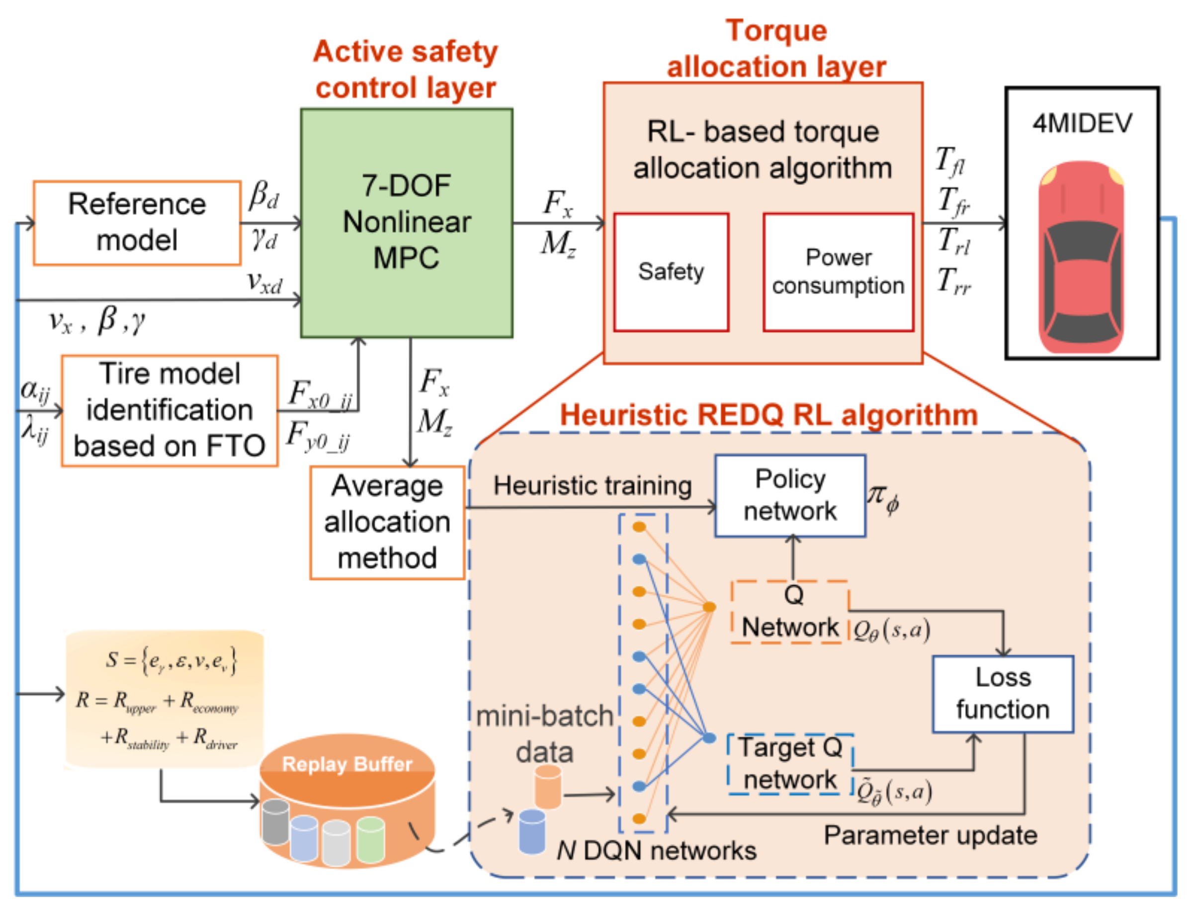
In the torque allocation layer, we considered a combination of safety and power consumption. In particular, the power consumption and safety weights are dynamically adjusted according to the current vehicle state based on RL. To this end, the task of this paper is the torque allocation of the 4MIDEV, which guarantees the safety and power consumption of the EV.

3.2.1. Average Allocation Method

As presented in references [18,25], the most common method of torque allocation is the average allocation method. The average allocation algorithm here serves two purposes. The first is as a base method for comparison. The second is as a heuristic training method for RL in the early stages of training. We have stated this in the revised manuscript. The average allocation methods are shown in the following [26]:
T f l = 1 4 F x R ω cos δ f + 1 4 M z R ω 1 2 d w cos δ f + a sin δ f T f r = 1 4 F x R ω cos δ f + 1 4 M z R ω 1 2 d w cos δ f + a sin δ f T r l = 1 4 F x R ω 1 4 M z R ω 1 2 d w T r r = 1 4 F x R ω + 1 4 M z R ω 1 2 d w

3.2.2. RL-Based Torque Allocation Algorithm

This section describes the details of the RL-based torque allocation algorithm. The state plays a crucial role in the RL algorithm, and in this study, we define the state space using four states: the yaw rate of deviation e γ = γ γ d e s , the stability indicator ε , velocity v , and velocity deviation e v . Additionally, the action is defined as four-wheel torque.
S = e γ , ε , v , e v , A = T f l , T f r , T r l , T r r
where the ε is obtained from the phase plane. In vehicle dynamics, the driving stability and instability regions can be depicted using a phase portrait [27]. The ε is defined as follows.
ε = β / B 2 + β ˙ B 1 / B 2
where B1 and B2 are the parameters associated with the adhesion coefficient. Their corresponding values are specified in reference [28]. This paper aims to improve the economy of EVs while ensuring safety, so the reward function R is expressed as the following four parts:
Firstly, Equations (29) and (30) ensure that the four-wheel torque satisfies the additional yaw moment M z and longitudinal force F x from the active safety control layer. Therefore, to ensure vehicle stability, the torque allocation layer needs to satisfy the following equation:
A s u c = B u
where A s = 1 R cos δ f cos δ f 1 1 l w 2 cos δ f + l f sin δ f l w 2 cos δ f + l f sin δ f l w 2 l w 2 , B u = F x M Z T , u c = T f l T f r T r l T r r T .
Therefore, we constructed R u p p e r to consider vehicle stability in the torque allocation layer from the perspective of the active safety layer:
R u p p e r = A s u c B u T W s A s u c B u
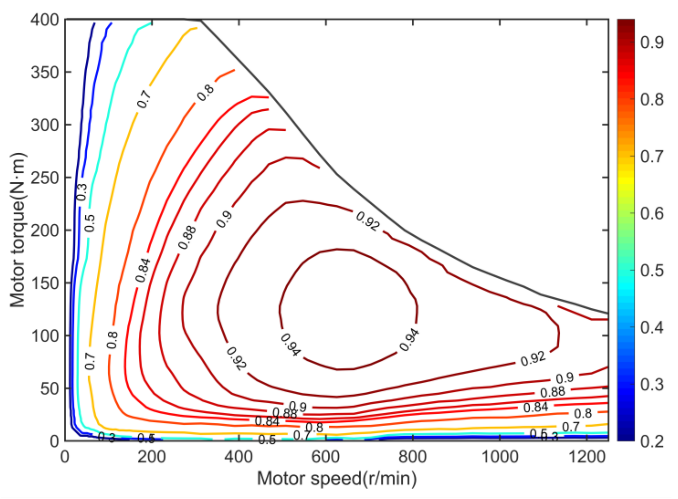
Second, the drive system power consumption is minimized by using the reward function Equation (36).
R e c o n o m y = W e c o n o m y i j = f l , f r , r l , r r P i j = W e c o n o m y i j = f l , f r , r l , r r T i j ω i j η T i j , ω i j
where W e c o n o m y is the penalty factors of economy, and ω i j is the speed of motor i j . Additionally, the motor efficiency η is shown in Figure 4.
Lastly, the stability indicators and driver load are considered in the reward function:
R s t a b i l i t y = W s t a b i l i t y β β d 2 + γ γ d 2 R d r i v e r = W d r i v e r δ ˙ s w 2 + W a _ δ a x 2
where W s t a b i l i t y and W d r i v e r are the penalty factors for safety and driver load, respectively.
R = R u p p e r + R e c o n o m y + R s t a b i l i t y + R d r i v e r
The safety of torque allocation consideration consists of two parts: R u p p e r and R s t a b i l i t y . As safety is the primary concern in vehicle operation, we chose penalty factors to ensure that the reward function satisfies the following relationship:
R upper + R stability s a f e t y > R e c o n o m y > R d r i v e r
The goal of the RL is to learn a policy that maximizes the expected cumulative reward over time. To encourage exploration and prevent premature convergence, the entropy term is included in the policy π :
π * = arg max π E τ ~ π γ f ( r t + ξ H ( π ( | s t + 1 ) ) )
where ξ is a temperature parameter that determines the level of exploration, and the additional entropy term H ( ) encourages exploration and prevents premature convergence to suboptimal policies.
Heuristic REDQ is an improved algorithm of REDQ. REDQ is a deep RL algorithm that combines ideas from both ensemble methods and double Q-learning to improve stability and sample efficiency [29]. In the REDQ algorithm, the Q function is expressed using the Bellman equation:
Q π ( s t , a t ) = E a t + 1 ~ π [ r t + γ f max a t + 1 Q π ( s t + 1 , a t + 1 ) + ξ H ( π ( | s t + 1 ) ) ]
where Q π ( s t , a t ) is the expected long-term reward of taking action a t based on policy π in state s t , r t = R ( s t ) is the immediate reward based on state s t , γ f [ 0 , 1 ] is the discount factor, s t + 1 is the next state after taking action a t in state s t , and a t + 1 is the next action.
To improve stability and reduce overestimation, the REDQ algorithm maintains an ensemble of N Q-networks, where each network is represented by a set of weights θ i , and the target value of Q-function is calculated by randomly selecting M Q-networks from N Q-networks:
y R E D Q = r t + γ f min m I M Q ˜ m ( s t + 1 , a t + 1 , θ ˜ t ) + ξ H ( π ( | s t + 1 ) )
where the set I M { 1 , 2 , , N } is M random elements.
The updated rule of evaluating Q-networks’ weights is by minimizing the loss:
L θ ( θ i ) = E ( s t , a t , r t , s t + 1 ) y R E D Q Q θ i ( s t , a t ) 2 , i = 1 , 2 , N
The target Q-networks are updated using a Polyak averaging:
θ ˜ i ρ θ ˜ i + ( 1 ρ ) θ i
where ρ is a hyperparameter that determines the smoothing factor.
In addition, the parameter ϕ of the policy π ϕ is trained by minimizing the loss:
L ϕ ( ϕ ) = E ( s t , a t , r t , s t + 1 ) 1 N i = 1 N Q θ i ( s t , a t ) + ξ H ( π ( a ϕ ( s ) | s t ) )
As the action here is the four-wheeled torque, its action space is four-dimensional, which adds difficulty to the training convergence of the agent. Therefore, a heuristic decay method is introduced here, with the final action being randomly chosen from the set of action strategies a O P , a r u l e with distribution 1 P r u l e , P r u l e . The probability of selecting action a r u l e is:
P r u l e = 1 tanh n r τ
where tanh ( x ) = e 2 x 1 e 2 x + 1 , n r is the cumulative number of runs, and τ is a constant that denotes the decay speed. The a r u l e is obtained from Section 4.1, and the a O P is expressed as:
a O P ( s t ) = tanh ( μ ϕ ( s t ) + σ ϕ ( s t ) φ ) T max
where φ ~ N ( 0 , I ) is an independent noise, μ ϕ ( s t ) is the mean of the stochastic policy that maps the state s t to an action, and σ ϕ ( s t ) is a random noise sampled from a probability distribution that encourages exploration. is the Hadamard product, and T max is the maximum motor torque, which is determined by the external characteristics of the motor.
To reduce overestimation and improve stability, REDQ uses an ensemble of Q-networks to estimate the Q-values and takes the minimum of the target Q-values from all the networks. To further improve sample efficiency, REDQ uses an update-to-data ratio denoted by G, which enables control over the number of times the data is reused. Algorithm 2 shows the detailed steps of the heuristic REDQ.
Algorithm 2. Heuristic REDQ algorithm
1. Initialize an ensemble of Q-networks Q θ ( s t , a t ) with parameters θ i , Set target parameters
2. Initialize the target Q-networks Q ˜ θ ˜ ( s t , a t ) with parameters θ ˜ i θ i
3. Initialize the replay buffer
4. For each step t do:
5.  Randomly sample an action a t from the set of action strategies a O P , a r u l e with distribution 1 P r u l e , P r u l e
6.  Execute the action a t and observe the next state s t + 1 , reward r t
7.  Store the experience tuple s t , a t , r t , s t + 1 in the replay buffer
8.  for G updates do
9.   Sample a mini-batch experiences s t , a t , r t , s t + 1 from replay buffer
10.   Randomly select m numbers from the set 1 , 2 , , N as a set I M
11.   Based on (42) compute the Q-value estimates y R E D Q
12.   for  i = 1 , 2 , , N   do
13.    Based on (43), update the parameters θ i using gradient descent method
14.    Based on (44), Update each target Q-network Q ˜ θ ˜ s t , a t
15.   end for
16.  end for
17. end for
18. Return the learned Q-network ensemble.

4. Evaluation Indicators and Simulation Results

4.1. Simulation Environment

To validate the effectiveness of the TVC algorithm, a joint simulation of CarSim, Simulink, and Python is used in this paper. The vehicle model in CarSim is based on the Magic Formula tire model. The vehicle model includes four in-wheel motors, which are controlled by the torque allocation algorithm implemented in Simulink. Python is used for training the RL algorithm. As the trained RL algorithm will not impose an additional computational burden on the TVC system, the main computational consumption of this paper lies in the nonlinear MPC. We have verified the real-time problem of the nonlinear MPC controller in the published paper [26], and the implemented nonlinear MPC algorithm by the ACADO toolkit [24], which has demonstrated its numerical efficiency for EV control in previous studies [5,30]. In this paper, the following five representative methods were selected for comparison and validation.
  • RLES. The torque allocation algorithm proposed in this paper. The active safety control layer is a nonlinear MPC controller, and the lower controller is based on a heuristic REDQ deep RL algorithm which integrates considering economy and safety.
  • MPC-CO. The torque allocation algorithm proposed in reference [26] which integrates considering economy and safety, where the lower controller is a quadratic planning algorithm.
  • LQR-EQ. The active safety control layer is the LQR controller in reference [31], and the torque allocation layer is a common average allocation method in Section 3.2.1. This controller considers vehicle safety only.
  • w/o control. There is no additional vehicle lateral control; steering is controlled by the driver.

4.2. Performance Indicators

To evaluate the effectiveness of the proposed torque allocation algorithm, several evaluation indicators are employed in this paper. These indicators include:
  • Handling stability
ε s = 0 t e β 2 + W β _ γ e γ 2 d t
where e β = β β r ,   e γ = γ γ r , and W β _ γ are the weights between e β 2 and e γ 2 .
2.
Driver workload
ε d r i v e r = 0 t δ ˙ s w τ 2 + W a _ δ τ a x τ 2 d τ
where a x is the longitudinal acceleration, δ s w is the driver steering wheel angle, and W a _ δ is the weight between δ ˙ s w 2 and a x 2 .
3.
Motor load
Frequent variations in motor torque may result in thermal saturation, which will increase the wear and tear on the motor.
ε m o t o r = 0 t Δ T f l τ 2 + Δ T f r τ 2 + Δ T r l τ 2 + Δ T r r τ 2 d τ
4.
Additional yaw moment
The magnitude of M z can represent the cost of stability control.
ε M z = 0 t M z τ 2 d τ
5.
Velocity tracking
Vehicle velocity is important for safety assessment, and ensuring vehicle safety while maintaining speed tracking is the goal of stability control.
ε v = 0 t v r e f τ v x τ 2 d τ

4.3. Training Performance

To ensure the performance of the controller under extreme conditions. We trained the RL agent in the lower controller on the simulation platform described in Section 3.2.2. The training condition is a low adhesion road with an adhesion coefficient of 0.3, and the vehicle velocity was increased from 60 km/h to 100 km/h in 10 s. The RL sampling time is 0.02 s, and the training time per episode is 10 s. The total number of training episodes is 800. The training results are shown in Figure 5.
The training reward curve of RL shows how the agent’s cumulative reward changes over the course of the training process. We can see that after about 580 episodes of training, the total rewards of the agent begin to converge at −65. During the early stages of training, the reward curve is erratic, with the agent sometimes achieving high rewards and sometimes achieving low rewards. As the agent learns and the training progresses, the reward curve gradually increases and stabilizes, indicating that the agent is becoming more proficient at the task.

4.4. DLC Maneuver on Slippery Road

The effectiveness of the proposed algorithm is tested under DLC conditions on slippery road surfaces. The longitudinal initial velocity is 72 km/h, and the tire–road friction coefficient is set as 0.3.
The vehicle trajectory in Figure 6a shows that the proposed RLES torque allocation algorithm provides better stability and control during the double line change maneuver compared to the MPC CO and LQR EQ controllers. The vehicle is able to maintain a smooth trajectory and quickly change its direction without large deviation or instability. Additionally, the vehicle under w/o control deviated significantly from the desired path. The yaw rate and side slip angle in Figure 6b,c also show improvements with the proposed RLES algorithm. The yaw rate and side slip angle of the RLES and MPC CO controllers can track the reference value throughout the maneuver, indicating good vehicle handling and control. The yaw rate and side slip angle in the LQR EQ and w/o controller show more oscillations and instability, which may cause the vehicle to lose control. The phase trajectory portrait in Figure 7a also proves this point.
The motor power consumption in Figure 7b also shows improvement with the proposed RLES controller. The motor power consumption is reduced, indicating better fuel economy. The other control strategies show higher motor power consumption, which may result in higher energy consumption and lower fuel economy. Compared to w/o control, RLES, MPC CO, and LQR EQ reduce motor power consumption by 80.2%, 78.4%, and 31.4%, respectively. Table 2 shows the results of the evaluation indicators for the four controllers. The RLES controller shows advantages for all indicators, especially for ε d r i v e r , ε m o t o r , and ε v .
Overall, the simulation results demonstrate the effectiveness of the torque allocation algorithm in improving vehicle stability, control, and fuel economy during a double-line change maneuver. This is because the RL-based RLES controller can learn the optimal strategy in continuous interaction with the environment and thus output the optimal four-wheel torque according to the current vehicle state.

4.5. DLC Maneuver on Joint Road

To simulate the condition of suddenly encountering an icy road surface at the start of a lane change and analyze the controller performance under extreme conditions, we set the road surface adhesion coefficient as Figure 8. Additionally, the target vehicle speed was 72 km/h, the EV was run in a DLC condition, and the reference trajectory is shown in the reference term in Figure 9a.
The trajectory of a vehicle controlled by RLES has a smaller displacement offset than other controllers as shown in Figure 9a. The vehicle can still complete the DLC maneuver under the w/o controller because of the decrease in vehicle speed, as shown in Figure 10b where the minimum speed of the w/o controller is 51 km/h. The side slip angle of the vehicle controlled by RLES was also well-controlled and remained close to zero, while the LQR EQ and w/o control controllers showed larger deviations from zero, indicating poorer vehicle stability, as shown in Figure 9c. The phase trajectory portrait in Figure 10a shows the relationship between the side slip angle and side slip angle rate, which demonstrates that the proposed RLES torque allocation algorithm provides better stability and control. The phase trajectory of the RLES is within the stability range, while the phase trajectory of the LQR EQ and w/o control controller exceeded the stability boundary and cannot return to the stability point, which may cause the vehicle to lose control.
Figure 11 shows the stability index and power consumption of the four controllers. It can be seen that both the RLES and MPC CO controllers perform significantly better than the LQR EQ and w/o controller. RLES and MPC CO improve the vehicle economy while ensuring vehicle safety. The performance of RLES is better than the MPC CO controller in terms of stability and power consumption, which indicates that the RLES based on RL training is suitable for different working conditions and can adaptively adopt the optimal control strategy according to the current vehicle state.
Table 3 summarizes the performance comparison of the four controllers. The simulation results demonstrate that the proposed RLES controller achieves superior performance in terms of power consumption, driver burden, and vehicle safety, making it a promising solution for the torque allocation of 4MIDEV.

4.6. Step Steering Maneuver

To verify the dynamic characteristics of the vehicle, a step steering maneuver was conducted for simulation validation. The vehicle was driving at a speed of 72 km/h on a good road surface with a road adhesion coefficient of 0.75. Within 0.5 s, the steering wheel angle increased from 0 deg to 120 deg and remained unchanged. The simulation results are shown in Figure 12 and Figure 13.
As shown in Figure 12a, the RLES control method shows relative understeering characteristics, which is beneficial for improving driver maneuverability. The yaw rate is shown in Figure 12b, indicating that both the RLES and MPC CO control methods could track the reference value well. Similarly, the side slip angle for the RLES and MPC CO control methods in Figure 12c is better than that of the LQR EQ and w/o control methods, and the RLES control method has the best maneuvering stability. Figure 13a shows the vehicle velocity variation curve in the step steering simulation, and the RLES method has better velocity tracking performance compared to other methods. The vehicle stability is improved under the RLES method while the longitudinal speed tracking performance is guaranteed. As seen in Figure 13b, except for the w/o control method, RLES consumed the least energy during the simulation. The w/o control method consumed the least energy because it does not require torque distribution to generate additional yaw moment by providing differential drive-assisted steering. However, this control method which sacrifices the vehicle stability is actually unsafe.
Table 4 shows the objective evaluation indicators under different controllers. It can be seen from the table that, except for the w/o control method, the RLES controller outperformed the other controllers in terms of vehicle stability, driver burden, and longitudinal speed tracking performance. In conclusion, the controller based on RLES not only ensures vehicle safety but also reduces the energy consumption of the drive system and improves economy under open-loop simulation conditions.

4.7. Driving Cycles

To evaluate the effectiveness of the proposed TVC algorithm in terms of energy savings, a series of tests were conducted under two different driving cycles: New European Driving Cycle (NEDC) and US06. The NEDC case was designed to simulate urban and high-speed driving scenarios, while the US06 driving cycle was designed to replicate a more aggressive driving behavior on the highway. Figure 14a depicts the vehicle velocity allocation for each driving cycle. Note that the driving cycle conditions do not include lateral control, so the performance of the LQR EQ controller is the same as without the control.
As depicted in Figure 15, the RLES algorithm increases the motor efficiency by 10.9% and reduces the motor power consumption by 11.0% compared to the LQR EQ algorithm in the NEDC cycle. This reduction in power consumption is achieved by optimizing the torque allocation strategy, thus allowing the motor to operate in the high-efficiency range as much as possible. In addition, the RLES also achieves optimal performance in the US60 driving cycle in Figure 15. These results demonstrate the RLES algorithm can adapt to different driving conditions and optimize the torque allocation strategy to achieve better energy efficiency.

5. Conclusions

The 4MIDEV has the feature of independently controllable four-wheel motors. To fully utilize this feature, the paper introduces a novel RL-based TVC algorithm for 4MIDEV that takes into account both economy and safety. The four-wheel tire model is identified using FTO with experimental data, and the active safety control layer utilizes a nonlinear MPC to calculate the required additional yaw moment and longitudinal force. The torque allocation layer employs a heuristic REDQ deep RL algorithm to compute the optimal four-wheel torque. The proposed RLES controller is validated and compared with typical MPC CO, LQR EQ, and w/o controllers under different driving scenarios. The results demonstrate that the proposed RLES enhances vehicle economy and reduces driver workload while ensuring vehicle safety. Future work will focus on designing a TVC algorithm for different driver steering characteristics and conducting real vehicle experiments.

Author Contributions

Conceptualization, H.D.; methodology, H.D.; software, Q.W.; validation, F.L.; formal analysis, Y.Z.; investigation, Y.Z.; writing—original draft preparation, H.D.; writing—review and editing, Y.Z.; supervision, Y.Z. All authors have read and agreed to the published version of the manuscript.

Funding

This research was funded by the Postgraduate Research and Practice Innovation Program of Jiangsu Province, grant number KYCX21_0188, the National Natural Science Foundation of China grant number 52272397, 11672127, the Fundamental Research Funds for the Central Universities, grant number NP2022408, and the Army Research and the National Engineering Laboratory of High Mobility anti-riot vehicle technology, grant number HTF B20210017.

Institutional Review Board Statement

Not applicable.

Informed Consent Statement

Not applicable.

Data Availability Statement

No external data were used in this study.

Acknowledgments

The authors gratefully acknowledge the financial support from the Postgraduate Research and Practice Innovation Program of Jiangsu Province (No. KYCX21_0188).

Conflicts of Interest

The authors declare no conflict of interest.

References

  1. Wu, J.; Zhang, J.; Nie, B.; Liu, Y.; He, X. Adaptive Control of PMSM Servo System for Steering-by-Wire System With Disturbances Observation. IEEE Trans. Transp. Electrif. 2022, 8, 2015–2028. [Google Scholar] [CrossRef]
  2. Wu, J.; Kong, Q.; Yang, K.; Liu, Y.; Cao, D.; Li, Z. Research on the Steering Torque Control for Intelligent Vehicles Co-Driving With the Penalty Factor of Human–Machine Intervention. IEEE Trans. Syst. Man Cybern. Syst. 2023, 53, 59–70. [Google Scholar] [CrossRef]
  3. Lei, F.; Bai, Y.; Zhu, W.; Liu, J. A novel approach for electric powertrain optimization considering vehicle power performance, energy consumption and ride comfort. Energy 2019, 167, 1040–1050. [Google Scholar] [CrossRef]
  4. Karki, A.; Phuyal, S.; Tuladhar, D.; Basnet, S.; Shrestha, B.P. Status of Pure Electric Vehicle Power Train Technology and Future Prospects. Appl. Syst. Innov. 2020, 3, 35. [Google Scholar] [CrossRef]
  5. Dalboni, M.; Tavernini, D.; Montanaro, U.; Soldati, A.; Concari, C.; Dhaens, M.; Sorniotti, A. Nonlinear Model Predictive Control for Integrated Energy-Efficient Torque-Vectoring and Anti-Roll Moment Distribution. IEEE/ASME Trans. Mechatron. 2021, 26, 1212–1224. [Google Scholar] [CrossRef]
  6. Chatzikomis, C.; Zanchetta, M.; Gruber, P.; Sorniotti, A.; Modic, B.; Motaln, T.; Blagotinsek, L.; Gotovac, G. An energy-efficient torque-vectoring algorithm for electric vehicles with multiple motors. Mech. Syst. Sig. Process. 2019, 128, 655–673. [Google Scholar] [CrossRef]
  7. Xu, W.; Chen, H.; Zhao, H.; Ren, B. Torque optimization control for electric vehicles with four in-wheel motors equipped with regenerative braking system. Mechatronics 2019, 57, 95–108. [Google Scholar] [CrossRef]
  8. Hu, X.; Wang, P.; Hu, Y.; Chen, H. A stability-guaranteed and energy-conserving torque distribution strategy for electric vehicles under extreme conditions. Appl. Energy 2020, 259, 114162. [Google Scholar] [CrossRef]
  9. Ding, S.H.; Liu, L.; Zheng, W.X. Sliding Mode Direct Yaw-Moment Control Design for In-Wheel Electric Vehicles. IEEE Trans. Ind. Electron. 2017, 64, 6752–6762. [Google Scholar] [CrossRef]
  10. Zhao, B.; Xu, N.; Chen, H.; Guo, K.; Huang, Y. Stability control of electric vehicles with in-wheel motors by considering tire slip energy. Mech. Syst. Sig. Process. 2019, 118, 340–359. [Google Scholar] [CrossRef]
  11. Zhang, L.; Chen, H.; Huang, Y.; Wang, P.; Guo, K. Human-Centered Torque Vectoring Control for Distributed Drive Electric Vehicle Considering Driving Characteristics. IEEE Trans. Veh. Technol. 2021, 70, 7386–7399. [Google Scholar] [CrossRef]
  12. Li, Q.; Zhang, J.; Li, L.; Wang, X.; Zhang, B.; Ping, X. Coordination Control of Maneuverability and Stability for Four-Wheel-Independent-Drive EV Considering Tire Sideslip. IEEE Trans. Transp. Electrif. 2022, 8, 3111–3126. [Google Scholar] [CrossRef]
  13. Deng, H.; Zhao, Y.; Nguyen, A.T.; Huang, C. Fault-Tolerant Predictive Control With Deep-Reinforcement-Learning-Based Torque Distribution for Four In-Wheel Motor Drive Electric Vehicles. IEEE/ASME Trans. Mechatron. 2023, early access. [Google Scholar] [CrossRef]
  14. Aradi, S. Survey of Deep Reinforcement Learning for Motion Planning of Autonomous Vehicles. IEEE Trans. Intell. Transp. Syst. 2020, 23, 740–759. [Google Scholar] [CrossRef]
  15. Zhu, Y.; Wang, Z.; Chen, C.; Dong, D. Rule-Based Reinforcement Learning for Efficient Robot Navigation With Space Reduction. IEEE/ASME Trans. Mechatron. 2022, 27, 846–857. [Google Scholar] [CrossRef]
  16. Kiran, B.R.; Sobh, I.; Talpaert, V.; Mannion, P.; Sallab, A.A.A.; Yogamani, S.; Pérez, P. Deep Reinforcement Learning for Autonomous Driving: A Survey. IEEE Trans. Intell. Transp. Syst. 2022, 23, 4909–4926. [Google Scholar] [CrossRef]
  17. Wei, H.; Zhang, N.; Liang, J.; Ai, Q.; Zhao, W.; Huang, T.; Zhang, Y. Deep reinforcement learning based direct torque control strategy for distributed drive electric vehicles considering active safety and energy saving performance. Energy 2022, 238, 121725. [Google Scholar] [CrossRef]
  18. Peng, H.; Wang, W.; Xiang, C.; Li, L.; Wang, X. Torque Coordinated Control of Four In-Wheel Motor Independent-Drive Vehicles With Consideration of the Safety and Economy. IEEE Trans. Veh. Technol. 2019, 68, 9604–9618. [Google Scholar] [CrossRef]
  19. Cabrera, J.A.; Ortiz, A.; Carabias, E.; Simon, A. An Alternative Method to Determine the Magic Tyre Model Parameters Using Genetic Algorithms. Veh. Syst. Dyn. 2004, 41, 109–127. [Google Scholar] [CrossRef]
  20. Alagappan, A.; Rao, K.V.N.; Kumar, R.K. A comparison of various algorithms to extract Magic Formula tyre model coefficients for vehicle dynamics simulations. Veh. Syst. Dyn. 2015, 53, 154–178. [Google Scholar] [CrossRef]
  21. Hu, C.; Wang, R.R.; Yan, F.J.; Chen, N. Should the Desired Heading in Path Following of Autonomous Vehicles be the Tangent Direction of the Desired Path? IEEE Trans. Intell. Transp. Syst. 2015, 16, 3084–3094. [Google Scholar] [CrossRef]
  22. Ji, X.; He, X.; Lv, C.; Liu, Y.; Wu, J. A vehicle stability control strategy with adaptive neural network sliding mode theory based on system uncertainty approximation. Veh. Syst. Dyn. 2018, 56, 923–946. [Google Scholar] [CrossRef] [Green Version]
  23. Zhang, H.; Liang, J.; Jiang, H.; Cai, Y.; Xu, X. Stability Research of Distributed Drive Electric Vehicle by Adaptive Direct Yaw Moment Control. IEEE Access 2019, 7, 106225–106237. [Google Scholar] [CrossRef]
  24. Houska, B.; Ferreau, H.J.; Diehl, M. An auto-generated real-time iteration algorithm for nonlinear MPC in the microsecond range. Automatica 2011, 47, 2279–2285. [Google Scholar] [CrossRef]
  25. Wang, J.; Luo, Z.; Wang, Y.; Yang, B.; Assadian, F. Coordination Control of Differential Drive Assist Steering and Vehicle Stability Control for Four-Wheel-Independent-Drive EV. IEEE Trans. Veh. Technol. 2018, 67, 11453–11467. [Google Scholar] [CrossRef]
  26. Deng, H.; Zhao, Y.; Feng, S.; Wang, Q.; Zhang, C.; Lin, F. Torque vectoring algorithm based on mechanical elastic electric wheels with consideration of the stability and economy. Energy 2021, 219, 119643. [Google Scholar] [CrossRef]
  27. Wu, X.; Zhou, B.; Wen, G.; Long, L.; Cui, Q. Intervention criterion and control research for active front steering with consideration of road adhesion. Veh. Syst. Dyn. 2018, 56, 553–578. [Google Scholar] [CrossRef]
  28. Zhai, L.; Sun, T.M.; Wang, J. Electronic Stability Control Based on Motor Driving and Braking Torque Distribution for a Four In-Wheel Motor Drive Electric Vehicle. IEEE Trans. Veh. Technol. 2016, 65, 4726–4739. [Google Scholar] [CrossRef]
  29. Chen, X.; Wang, C.; Zhou, Z.; Ross, K. Randomized Ensembled Double Q-Learning: Learning Fast Without a Model. arXiv 2021, arXiv:2101.05982. [Google Scholar]
  30. Parra, A.; Tavernini, D.; Gruber, P.; Sorniotti, A.; Zubizarreta, A.; Perez, J. On Nonlinear Model Predictive Control for Energy-Efficient Torque-Vectoring. IEEE Trans. Veh. Technol. 2021, 70, 173–188. [Google Scholar] [CrossRef]
  31. Mirzaei, M. A new strategy for minimum usage of external yaw moment in vehicle dynamic control system. Transp. Res. Part C Emerg. Technol. 2010, 18, 213–224. [Google Scholar] [CrossRef]
Figure 1. The block diagrams of the TVC system.
Machines 11 00459 g001
Figure 2. Tire model identification results. (a) Longitudinal force recognition results. (b) Lateral force recognition results.
Machines 11 00459 g002
Figure 3. Vehicle 7-DOF dynamic model diagram.
Machines 11 00459 g003
Figure 4. Motor efficiency map.
Machines 11 00459 g004
Figure 5. RL algorithm training reward curve.
Machines 11 00459 g005
Figure 6. Simulation results on slippery road. (a) Vehicle displacement; (b) yaw rate; (c) side slip angle.
Machines 11 00459 g006
Figure 7. Simulation results on slippery road. (a) Phase trajectory portrait; (b) motor power consumption.
Machines 11 00459 g007
Figure 8. Adhesion coefficient of the joint road.
Machines 11 00459 g008
Figure 9. Simulation results under joint road. (a) Vehicle displacement; (b) yaw rate; (c) side slip angle.
Machines 11 00459 g009
Figure 10. Simulation results under joint road. (a) Phase trajectory portrait; (b) longitudinal velocity.
Machines 11 00459 g010
Figure 11. Simulation results under joint road. (a) Stability index ε s ; (b) motor power consumption.
Machines 11 00459 g011
Figure 12. Simulation results under step steering maneuver. (a) Vehicle displacement; (b) yaw rate; (c) side slip angle.
Machines 11 00459 g012
Figure 13. Simulation results under step steering maneuver. (a) Longitudinal velocity; (b) motor power consumption.
Machines 11 00459 g013
Figure 14. Velocity distribution of driving cycles. (a) NEDC; (b) US06.
Machines 11 00459 g014
Figure 15. Simulation results under driving cycles. (a) Motor efficiency; (b) motor power consumption.
Machines 11 00459 g015
Table 1. First-level parameters identification results.
Item10 kN15 kN20 kN
FTO relative residual of longitudinal force1.40%1.37%1.40%
GA relative residual of longitudinal force4.61%2.21%1.73%
PSO relative residual of longitudinal force3.44%1.74%1.66%
FTO relative residual of lateral force1.48%1.37%1.39%
GA relative residual of lateral force1.78%1.63%1.48%
PSO relative residual of lateral force1.65%1.69%1.56%
Table 2. Performance indicators in DLC maneuver on slippery road.
Controller𝜺s𝜺driver𝜺motor𝜺Mz𝜺v
RLES0.4085−96%16.28−81%20,820−93%735,2001.1 × 10−5
MPC CO0.5640−94%19.58−77%23,430−92%887,2001.5 × 10−5
LQR EQ3.6532−61%32.54−62%29,680−90%892,0003.5 × 10−4
w/o control9.260-85.46-306,300-02.9 × 10²
Table 3. Performance indicators in DLC maneuver on joint road.
Controller𝜺s𝜺driver𝜺motor𝜺Mz𝜺v
RLES0.5574−94%16.28−81%20,820−93%735,2000.88
MPC CO0.6368−93%19.58−77%23,430−92%887,2001.42
LQR EQ4.2190−57%32.54−62%29,680−90%892,0002.47
w/o control9.707-85.46-306,300-036.78
Table 4. Performance indicators in step steering maneuver.
Controller𝜺s𝜺driver𝜺motor𝜺Mz𝜺v
RLES0.0183−62%42.46−1.7%99301 × 1070.01895
MPC CO0.0193−60%42.46−1.7%98731 × 1070.0273
LQR EQ0.0274−43%43.210.1%4166170,1000.04486
w/o control0.0483-43.18-132.702.202
Disclaimer/Publisher’s Note: The statements, opinions and data contained in all publications are solely those of the individual author(s) and contributor(s) and not of MDPI and/or the editor(s). MDPI and/or the editor(s) disclaim responsibility for any injury to people or property resulting from any ideas, methods, instructions or products referred to in the content.

