1. Introduction
The demand for advanced technology has increased due to the growing popularity of multi-robot systems in industry and warehouses for logistics tasks. These systems are essential for performing tasks that cannot be handled by a single robot, and are more cost-effective and durable than specialised robots [
1]. This makes them ideal for use in flexible manufacturing cells or automated warehouses [
2,
3,
4]. However, the current challenge is to effectively manipulate objects with mobile robots in large warehouses. Non-inertial multi-robot systems offer a solution to this problem, as they can operate in a much larger workspace than inertial robots. Among mobile robots, holonomic robots have proven to be effective in performing manipulation tasks in various applications, such as material handling, warehouse management, and assembly line production. These robots have high flexibility and manoeuvrability as they can move in any direction and orientation. However, the design and control of such robots can be challenging, requiring careful consideration of the robot’s dynamics and control algorithms to ensure safe and effective manipulation of objects [
5]. Despite this advantage, there is still a need to enable them to manipulate a wider range of object types with specific end effectors [
6,
7]. Further research is needed to improve the efficiency of these systems and to overcome any challenges that may arise during their deployment.
Manipulation by caging refers to a method of controlling groups of robots to interact with and manipulate objects in the environment [
8]. This method is based on the idea of surrounding and holding an object with the action of multiple robots. This approach offers several advantages over traditional manipulation methods, such as increased stability, robustness to external disturbances, and the ability to manipulate objects with complex shapes and textures. To achieve this type of manipulation, it is often necessary to break it down into simpler behaviours. These behaviours may include establishing and maintaining contact between the manipulators and the object, moving the object to a desired position, and releasing the object. In this paper, we focus on a manipulation scheme that is capable of manipulating regular cylindrical objects rather than those with complex shapes. Although complex figures may require more sophisticated manipulation techniques, regular shaped objects are more common in warehouse environments and can be manipulated efficiently using simple grasping and manipulation strategies. In addition, the perception and localization required for the manipulation task are simplified because regular objects are easier to recognize and track in the environment. Therefore, our decision to focus on regular shaped objects is motivated by the practical considerations of warehouse applications. Nevertheless, the proposed manipulation scheme can be extended to handle more complex shapes by incorporating additional perception and planning capabilities.
Transition processes are useful for coordinating cooperative behaviour in a multi-robot system. Specifically, the transition process is a sequence of specific behaviours, whose fulfilment in the correct order contributes to the performance of a specific task autonomously. In a multi-robot system, the autonomy of the transition process is attained by integrating a decision agent that manages the transition between the behaviours executed by each robot during the process [
9,
10]. In Ref. [
11], a solution is proposed to integrate a transition agent using flags to change the system behaviour. This behaviour consists of task sequences, moving groups of robots between work areas, but relies heavily on sensor precision due to error dependence [
12,
13,
14]. Additionally, the described solution increases the complexity of working with groups of tasks. From here, the problem of the phase transition arises, which has been worked on in Ref. [
15], where a kinematic controller capable of handling several conflicting tasks in a multi-robot system is proposed; this proposal considers the performance of both cooperative tasks as well as individual tasks. In Ref. [
16], a task set is proposed for object handling and transportation. The method utilizes internal distances between robots to form relatively rigid formations, ignoring clamping methods. The transition process is managed by a state machine, the transition agent, which changes the state based on a metric determined by the designer. In consequence, the system’s reliability depends on the operator’s knowledge and the sensitivity of the sensors. Regarding the task transition planning, the authors in Ref. [
17] focus on the task planning aspect of home service robotics, where sequences of actions are generated to complete tasks based on high-level and low-level actions. However, unlike classical planning methods, task planning in the home environment is fraught with uncertainty and change, which requires consideration of human–robot interactions. In addition, this paper discusses the challenges and current approaches to accomplish the task under uncertain and incomplete information. In Ref. [
18], a dynamic control for mobile robots with an integrated manipulator is presented. This work proposes a robust controller that ensures finite-time convergence of the error in the presence of parametric uncertainties. The work integrates a finite-state machine (FSM) with transitions of predetermined lapses. This type of FSM works only under the premise that the predetermined transition time is greater than the convergence time of the system.
Our proposed scheme focuses on transitions as events in a probability space and utilizes measurements to adjust the probability measure of each event to formulate a stochastic control system. Stochastic systems are well-suited for scenarios where the phenomenon under investigation is influenced by unpredictable factors. They have been applied in the field of multi-robot systems, resulting in innovative navigation approaches in stochastic environments (such as wind currents and flexible patterns) [
19,
20]. In Ref. [
21], the authors analyse network applications and information processing, where access to information depends heavily on human interaction. To enhance this, a medium access control based on stochastic models is proposed to improve the management of information flow. In Ref. [
22], a Markov chain-based methodology is proposed to define system behaviour subject to random forces. Additionally, in Ref. [
23], the authors present a control design for stochastic perturbations using observer-based output feedback with a Markov chain and the invariant ellipsoid approach.
Following this line of research, it is necessary to find useful qualities to analytically evaluate a stochastic system. In our proposal, stability in the mean-square sense was adopted. This stability notion is a deeply studied quality of the behaviour of stochastic differential systems, which is used to demonstrate the desired properties of such systems [
24,
25]. In Ref. [
26], the mean square lemma is analysed. It shows, through system causality, that having a bound on the mathematical expectation of the state, output, or stochastic phenomenon is sufficient to prove mean-square stability of the entire closed-loop system [
27].
The main contribution of this paper is the development of a novel decision agent, represented by a discrete-time Markov chain (DTMC), which ensures the stability of a comprehensive manipulation scheme. This scheme uses information from the environment and a group of robots to execute a set of behaviours that achieve the goals of the manipulation task [
28]. Furthermore, our proposal is robust to uncertainties that may occur during the manipulation, keeping the desired behaviour according only to the actual conditions of the task, which makes it more reliable and applicable to real-world scenarios. Additionally, a stability analysis of the manipulation scheme is presented, demonstrating that the mathematical distribution of the DTMC is dependent on the error of the robot task and the resulting closed-loop system is stable in a mean-square sense, thereby confirming the stability of the manipulation scheme.
The paper is organized as follows.
Section 2 presents the methodology of the proposed manipulation scheme.
Section 3 describes the equations of motion of the multi-robot system.
Section 4 details the tasks that the multi-robot system can perform. Then,
Section 5 shows how to deal with tasks simultaneously with hierarchical quadratic programming (HQP).
Section 6 explains how the tasks are grouped in a space defined as “action phases”.
Section 7 describes the construction of a Markov chain with a state-measure-dependent distribution.
Section 8 shows simulations that support the operation of the complete scheme, demonstrating that the proposed DTMC decision agent provides significant improvement in performance when compared with a FSM agent. Finally, the conclusions of the work and future work based on the results of this research are presented in
Section 9.
2. Manipulation Scheme
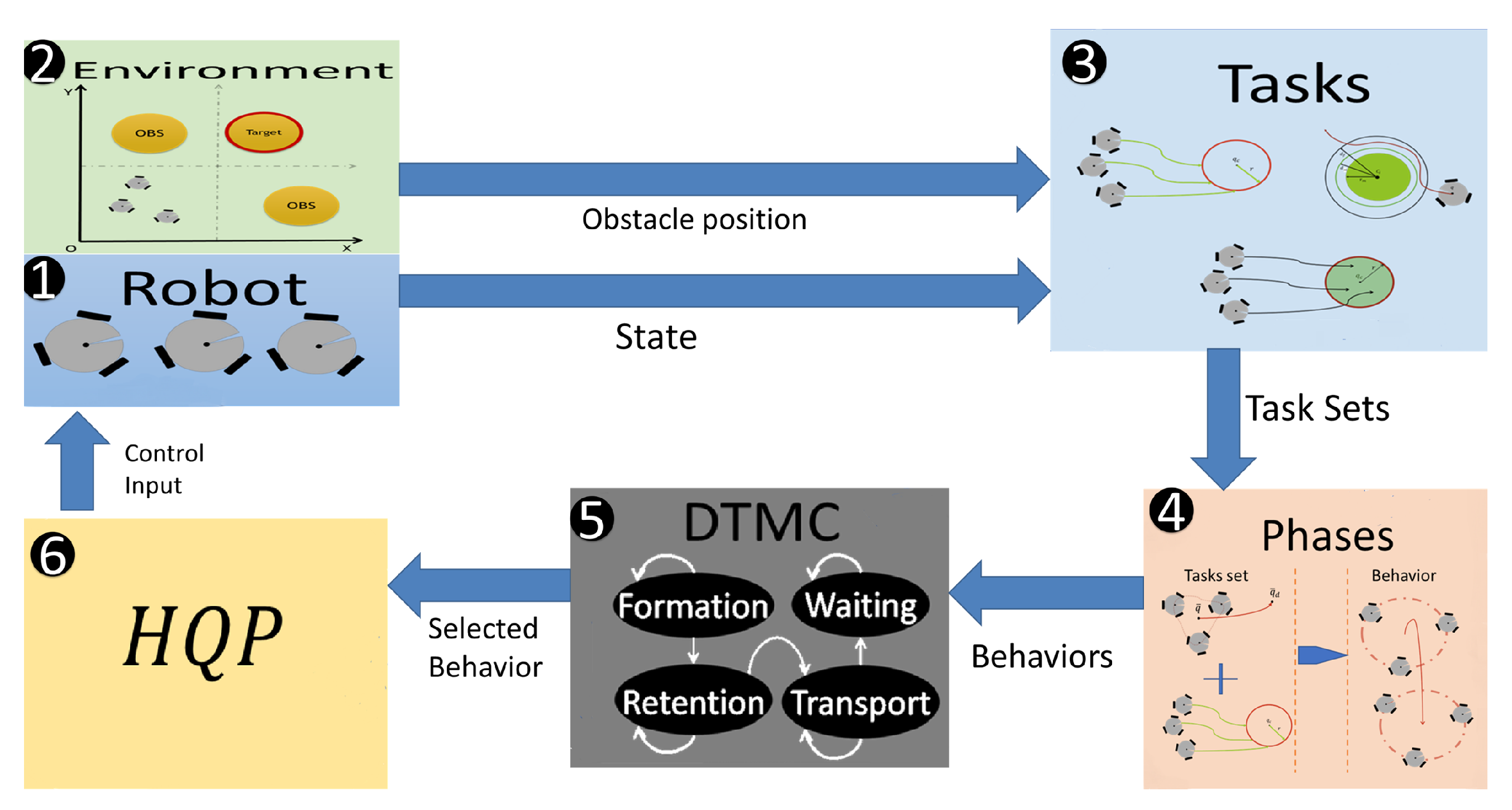
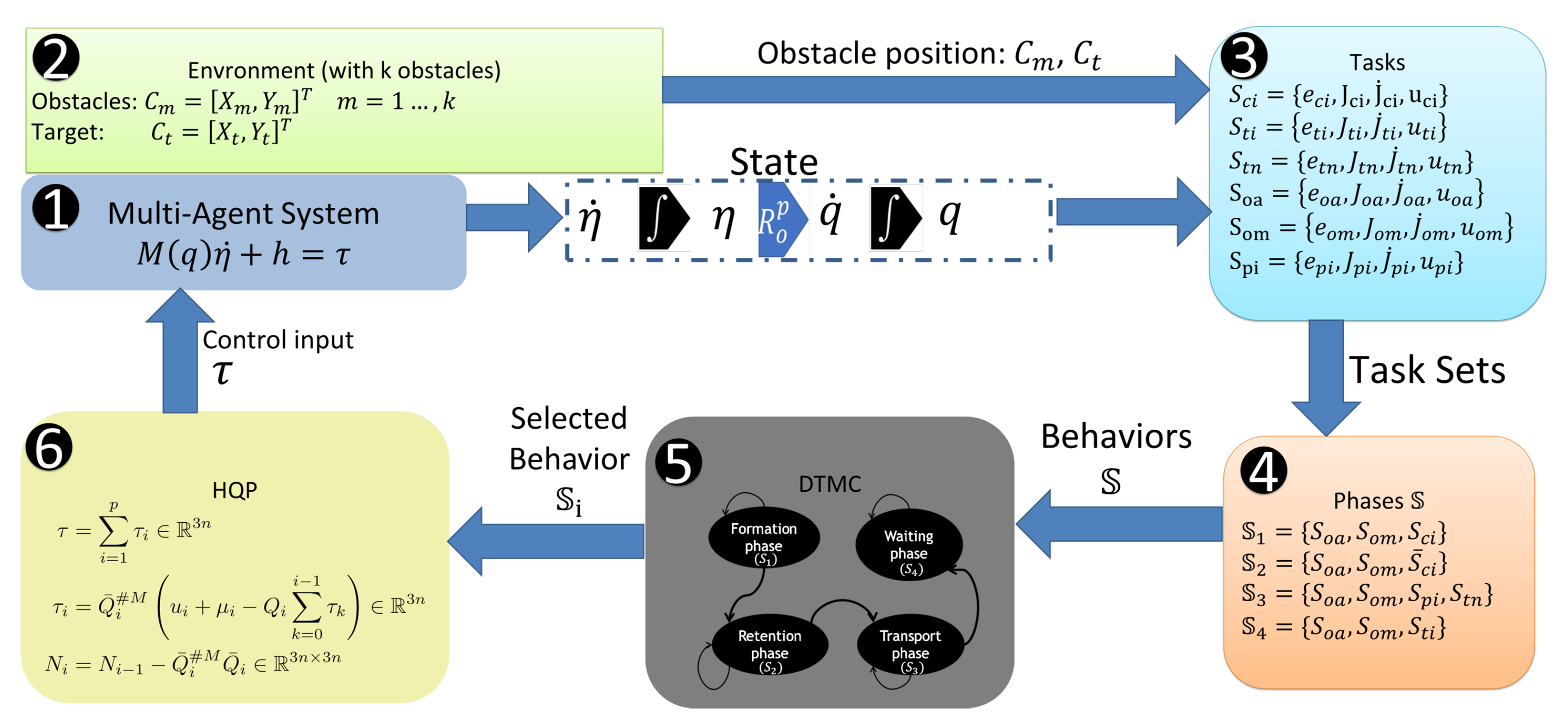
The methodology involved in constructing the manipulation scheme consists of six process blocks: Robot, Environment, Tasks, Phases, DTMC, and finally HQP. The blocks are connected as shown in
Figure 1. In the Robot block, the dynamic model of the multi-robot system is found, from which the state of all the agents in the system is obtained. In the environment block all the information of the workspace and the assignment of objectives of the scheme are defined, such as the position and size of the obstacles, the selection of the objective, and the desired position of the objective. The Tasks block obtains the values of the tasks available to the multi-robot system in the form of errors, whose minimization represents the fulfilment of the task. The tasks are computed with the information of the environment and robots, which includes both cooperative and individual tasks. In the Phases block, tasks are grouped into distinct phases, defining the necessary behaviour for the robot to perform the target manipulation process. The DTMC process block has a transition agent, represented by a DTMC, which selects a Phase based on the completion of the previous one, as it uses a state-measured probability distribution. Finally, the HQP block generates a control input to the multi-robot system that seeks the fulfillment of the tasks contained in the selected phase simultaneously.
In the context of modelling our decision agent, it is important to choose a suitable mathematical model that can maintain consistent performance despite potential uncertainties. While conventional DTMC and FSM are common mathematical models for discrete systems, modelling decision agents requires selecting a model that can effectively address robustness to unexpected events and consider its limitations. Our focus is on DTMC as it has been shown to be effective in handling uncertainties and randomness [
23,
29]. On the other hand, FSM, which relies on deterministic rules, is limited in its ability to model probabilistic behaviour [
15,
18], and constructing an accurate FSM-based decision agent can be complex and requires specialized knowledge of the system. Despite this, the proposed manipulation scheme has the disadvantage of requiring a simultaneous transition of the behaviour of each of its agents. Therefore, without reconsidering a more specialised Markov chain, it is currently not possible to implement it in a decentralised manipulation scheme.
We implement this scheme in a simulation study by considering a group of Festo Robotinos. We chose these robots since they represent a versatile and powerful mobile robot platform suitable for a wide range of applications, including material handling, warehouse management, and research [
30]. The Robotino’s omniwheels provide smooth and accurate motion, enabling precise positioning for object manipulation.
3. Dynamic Model
For implementing the scheme, the Robot block represents a group of
n omnidirectional robots, with its dynamic model. The notation used in the scheme is presented in
Table 1. The position and orientation of this group of robots is represented by
, where
is the position and orientation of the mobile frame
attached to the centre of the
i-th robot, with respect to the inertial frame
O. Let us define the rotation matrix
as
then, for a total representation of the system, it is defined
which is the block-diagonal matrix that relates the frame
P to the frame
O. To determine the velocities of each of the
n robots in the
P frame, we introduce the space
with
defined as
where
is the transpose of the rotation matrix from frame
P to
O at orientation
, and
is the velocity of the
i-th robot in the
O frame.
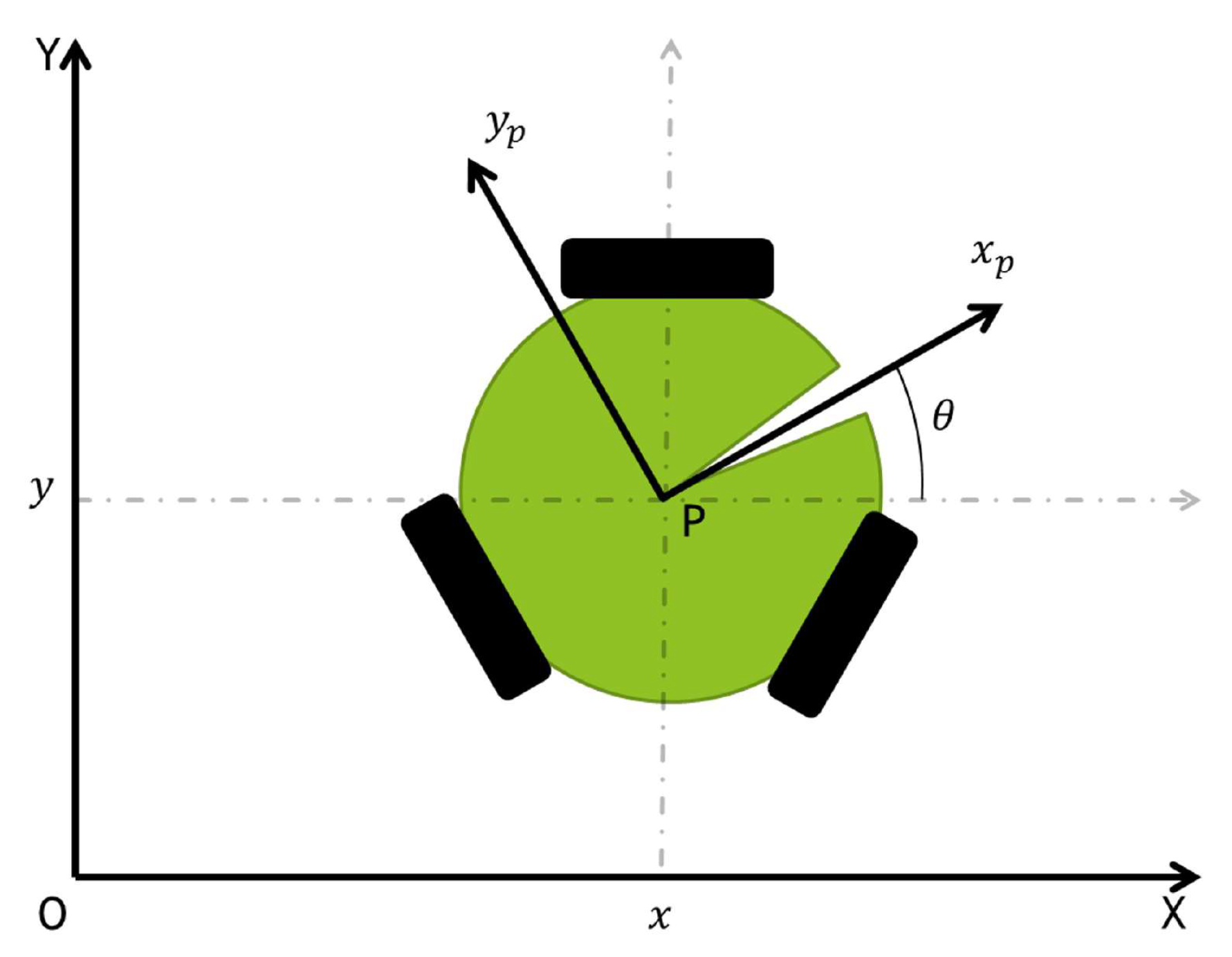
These robots have an omnidirectional configuration that is achieved with three holonomic wheels coupled equidistant around the main body [
5]. In order to better understand the mathematical representation of the robot, the variables used in (
4) are described in
Table 1. The robot seen in
Figure 2 is represented mathematically by
where the matrix
E encodes the wheel configuration and represents the holonomic wheel projection as
where
b is the distance between the robot centroid and the wheel, and
is the radius of the wheel
i.
A compound system is defined to represent the dynamic behaviour of a group of robots,
5. Hierarchical Quadratic Programming
HQP is capable of handling multiple hierarchical objectives while ensuring that kinematic and dynamic constraints are satisfied, and provides a computationally efficient solution by decomposing the problem into a hierarchy of sub-problems and solving them iteratively. This allows us to ensure that the robot’s motion satisfies all the constraints, while dealing with multiple objectives at different levels of the hierarchy.
A group of the tasks described in
Section 4 can be performed simultaneously by the multi-robot system in each of the phases of the scheme, so HQP is used to find a control input
, applied in (
6), which fulfils all the tasks included in a phase. The main characteristic of HQP is that lower priority tasks cannot affect higher priority tasks by solving a quadratic programming cascade with slack variables. The main idea is to find a control signal that obeys a set of
p tasks to be executed simultaneously, as shown in the Algorithm 1.
Consider the double integrator system
and
as a PD control law
, which is needed for HQP of the tasks defined in
Section 4 [
18]. The tasks are considered an error function of the form
We assume that (
26) is twice differentiable with respect to time
From (
6) and (
27), we obtain
where
and
is the task’s drift. The task-based inverse dynamic is obtained by solving for
in (
28) as follows:
is the weighted generalized inversion of
, and
u is the auxiliary vector of control inputs. To overcome possible conflicts among the tasks, the hierarchy between them is imposed such that (
29) becomes:
where
,
,
and
. Notice that
belongs to the null space of
.
| Algorithm 1 Task phase |
- Require:
State of the group (), Task phase , - Ensure:
Control input
Indicate the order of the tasks: Get task Jacobians: Get time derivative task Jacobians: |
6. Action Phases
Each phase requires specific behaviour in the robots. Depending on the task, the robots can work as a team or individually. However, they are always reacting to their environment for obstacle and collision avoidance tasks.
The action phase
is a set of tasks introduced in the HQP block to be fulfilled in a defined hierarchy. Each Action phase considers the sets of task errors, task projector Jacobians, the time derivative from the projector Jacobians, and a set of auxiliary control inputs that asymptotically minimize each error of the Action Phase. The
i phase of action is arranged in the group
. For the purpose of this paper, four phases of action are considered, presented in
Table 2,
The evaluation of whether tasks are fulfilled is measured through the error generated by each task. A task is considered accomplished when its error remains in a neighbourhood close to zero. Likewise, a phase is considered to be reached when the errors of all its tasks are fulfilled. It is considered a state composed of the errors generated in the phase,
This state exists in a normed space of the phase whose vector norm provides us with substantial information about the development of the task at each time step. A norm is proposed in order to have an analytical perception of the behaviour of the vector in a scalar way, even when the dimension of the vector changes between the existing phases in the totality of the process.
7. Discrete-Time Markov Decision Agent
Definition 1 (Probabilistic space). Let Ω be a space with a family of subsets (in this paper it is considered as the set ), such that any subset is closed under accounting complements, unions, and intersections. A family of subsets possessing these properties is known as a algebra. If a probability measure P is defined on the σ-algebra , then the triple is called a Probability space and the sets in are called random events.
Definition 2 (Markov condition).
Consider a probability space from Definition 1 . Let E be a finite or countable set of states and a sequence of random variables. The process is said to satisfy the Markov condition if for all integer and all that belongs to E, it holds: Definition 3 (Distribution by state measure).
Let E be a countable set. Each is called a state and I is called a state space. We say that a subset , where , is a measure on E∀. We work with a probability space from Definition 1, a random event Ξ
that takes values of and a random event with values in E. Then, it is said that α defines a distribution by state measure if it satisfies the condition: Definition 4 (Mean-square stability).
Let , if for every , there exist such that for all whenever then it is said that X is stable in mean-square sense [31]. The Markov chain is a discrete-time stochastic process in which a random variable that takes values of
changes over time. Its main characteristic is that it complies with the Definition 2 [
22]. The measurement of the phase for the system comes from the error vector of (
32). Likewise, the norm
is proposed as a decision agent to affect the transition matrix. A bounded exponential function is generated to provide information about the tasks in each phase and ensure that the task has been completed before each transition. This function depends on
,
Notice the non-negative nature of the vector norm and the exponential envelope of the function
. A new transition matrix is defined, where the probability of task development is based on relevant state measurement information for each element,
where
,
is the nominal probability,
m is the number of states in the system, and
T is the current instant of the system. This obeys the requirement of a transition matrix where the sum of the elements of each row is 1. After finding
, it is balanced with the complement probability, forcing
with (
36), this
of State 1 is considerably small, the measurement
of State 2 is the complement and therefore takes higher values.
Theorem 1. Let a decision agent be represented by a probabilistic space and fulfil the Markov condition with distribution by state measure as Definition 3. Then is stable in mean-square sense according to Definition 4.
Sketch of the Proof. Once the decision agent, represented by a Markov chain, selects a phase
, we obtain an error
and therefore the computation of a control
, which is applied to the robot to minimize that error. Since
measures the phase error
, it will change as the error converges to zero. Given the
from (
35), there is a direct proportion relationship with
, if the error takes values close to 0 then
in phase
is close to 0, ensuring the existence of
. Since there are a limited number of transitions from the current state, according to Definition 3,
exists in every moment and implies that
is less than or equal to the number of possible transitions that exist in each phase. Then
and
from Definition 4 always exist, which implies that the proposed decision agent is stable in the least-squares sense. □
The manipulation scheme is considered a stochastic system when it operates in a closed loop since the random variable of the decision agent is being fed back. Therefore, it is important to demonstrate the stability of the system with stochastic tools. The stability presented in the decision agent ensures that the stability in the mean-squares sense is preserved in the rest of the processes thanks to the causality of the events in the whole manipulation scheme.
8. Simulation Results
To test the validity of the proposed manipulation scheme, which is described in
Figure 9, numerical simulation results are presented. The simulator was programmed in Python3, on a computer equipped with an Intel® Core™ i7-8565U CPU @ 1.80 GHz and 8 GB RAM. The Markov chain’s transition probability is set at a 0.01 second sampling time, affecting the duration of each phase. Each phase is expected to last 1500 steps with this transition probability design. This means that the probability of staying in phase
is
, which implies that the initial transition probability is
. Wheeled robots with a mass of
m = 1 kg, an inertia tensor of
kgm, as well as an inertia tensor of the wheels of the wheeled robot of
kgm, and a radius of
m, are considered. There are obstacles at
and
with a radius of
m.
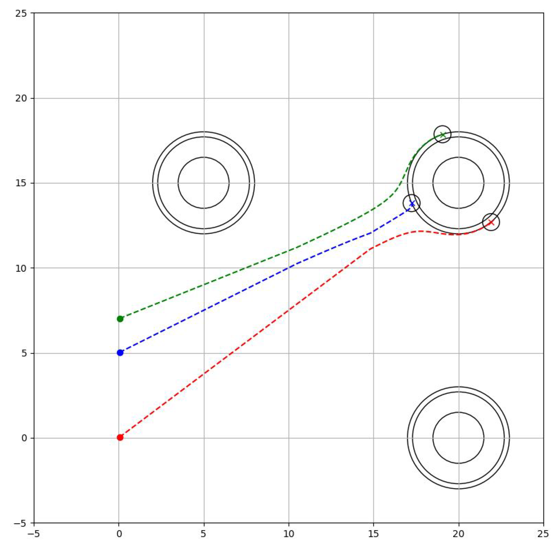
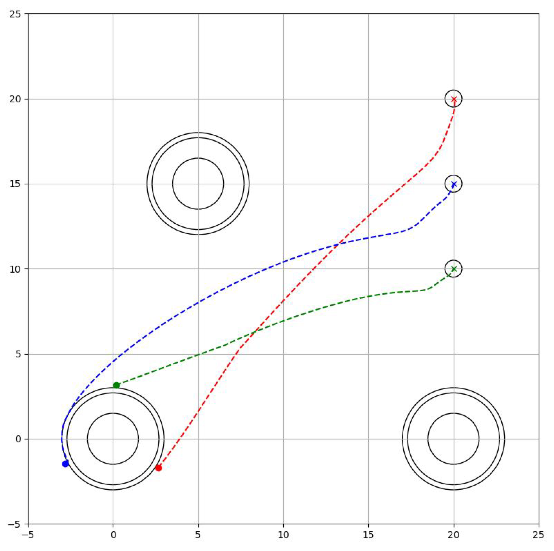
8.1. Phase 1: Formation Phase
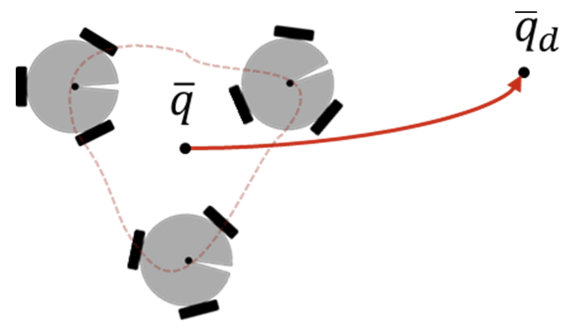
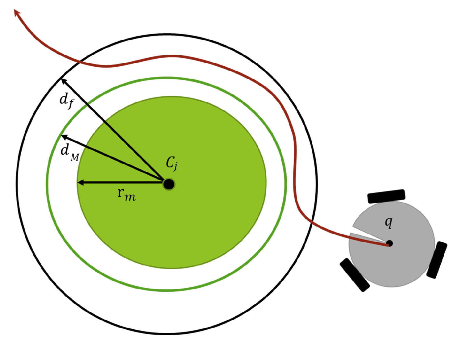
The robots are directed from their starting position to the border with the target (
), where strict avoidance of the obstacles and collision between them is important (
). Therefore the task Phase is designed as
where
is the radius of the robots and
is the security distance of the obstacles, which indicates that
is more important than
. The resulting trajectory is seen in
Figure 10.
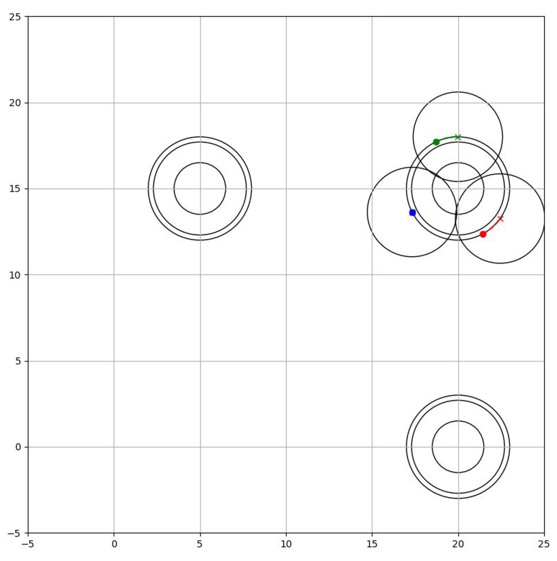
8.2. Phase 2: Grip Phase
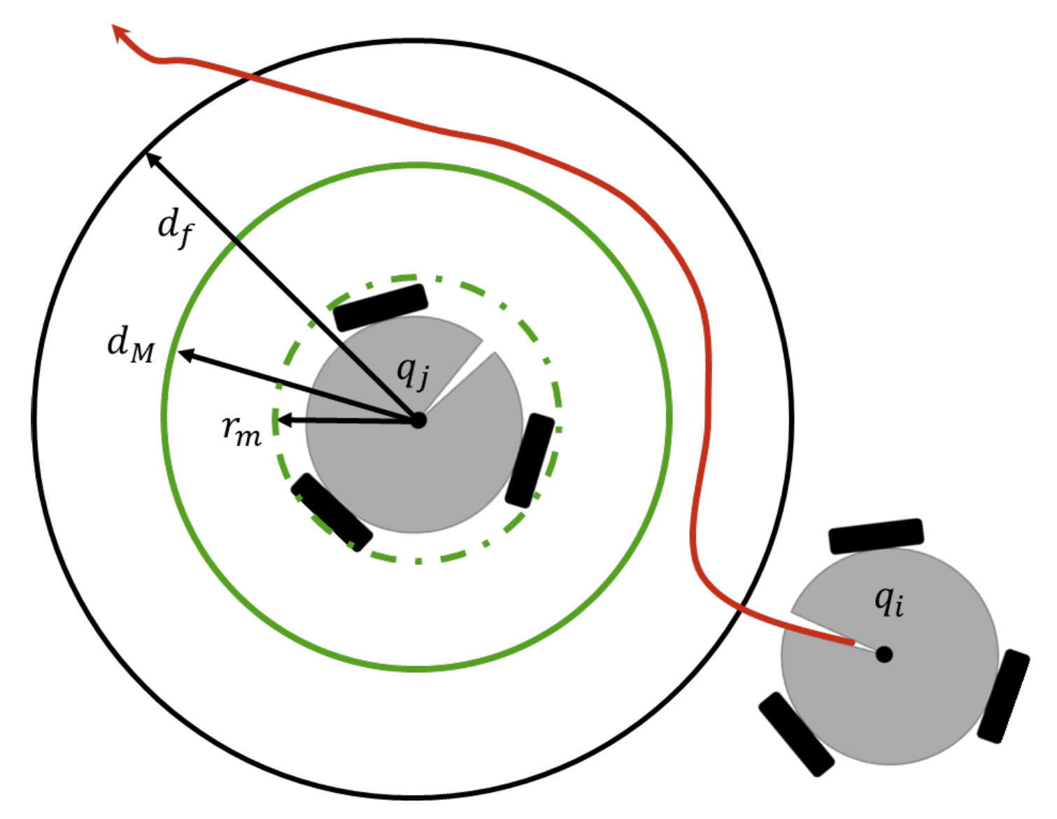
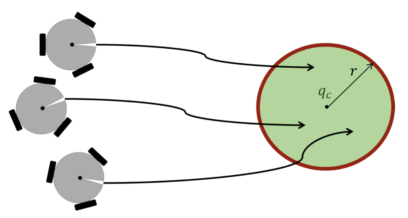
The robots must ensure that the object they are going to hold is kept in the centroid of the formation, therefore, they must avoid the target space without separating from it, while separating equally from each other. The task to accomplish is practically the same as the first phase, however, they need to take a greater distance to avoid collisions between the robots. Then
where
is the distance needed in order to form a circumscribed triangle towards the objective as seen in
Figure 11.
8.3. Phase 3: Manipulation Phase
Robots must maintain the desired permissible space in the formation while avoiding obstacles on the stage. The task is completed when they move the object, that is, the centroid of the formation to the desired position. Thus, the task phase becomes
Notice that the formation can avoid also the target to move since it is logically considered an obstacle.
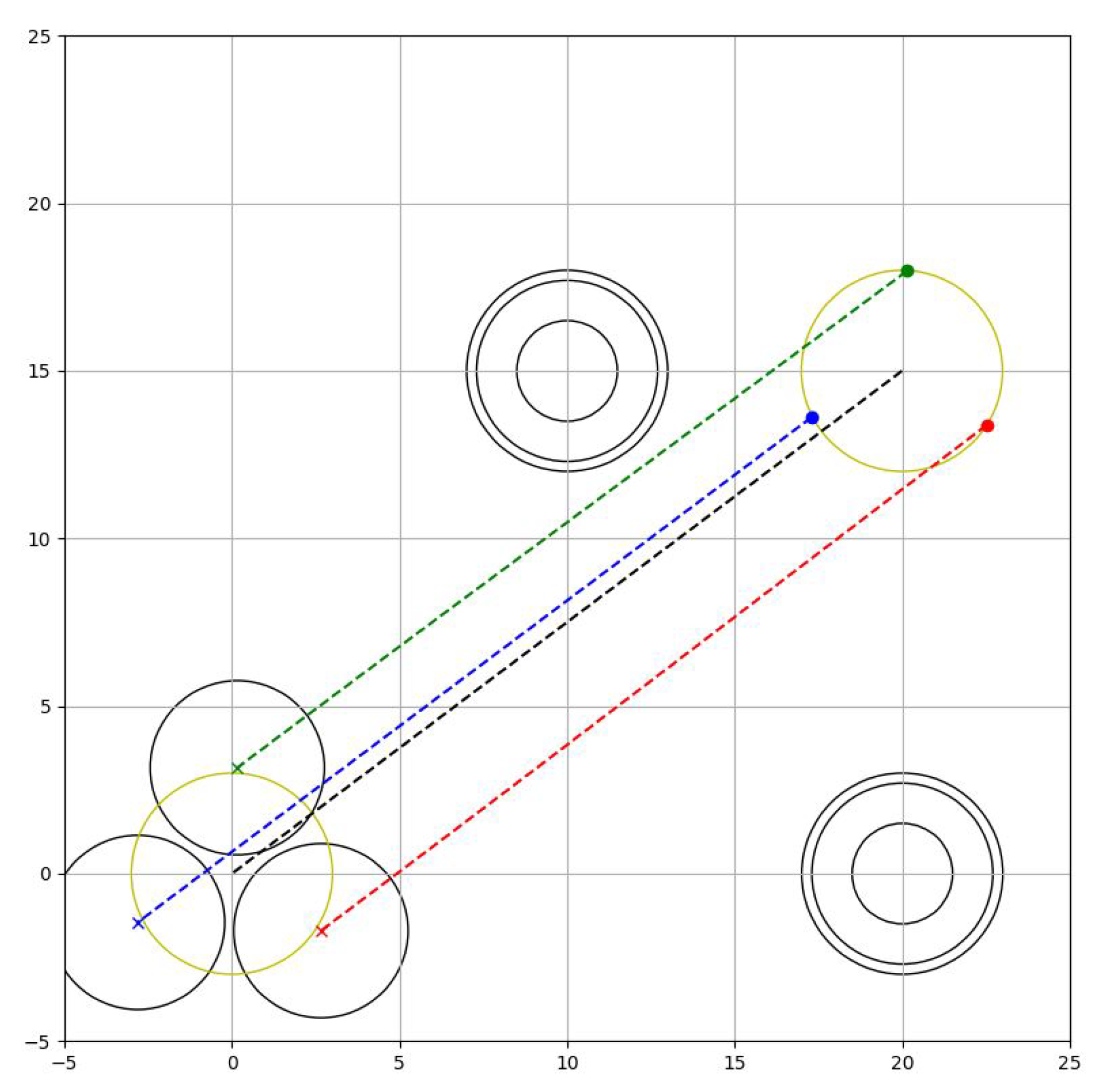
8.4. Phase 4: Waiting Phase
Once the robots have moved the target to the desired location, they separate from it and head towards a pre-defined obstacle-free position, in order to finish the job or wait for a new target. The task phase becomes
Notice that in all the tasks one of the priorities is that the robots strictly avoid the obstacles, therefore it would be a task of greater importance in all the phases. Although the tasks of lower priority are projected into the null space of the stricter tasks, they find a close solution for each of the tasks.
8.5. Variance Value and Phase Measure
The closed-loop system becomes a differential stochastic system. Therefore, the stability analysis of the system has to consider tools applied in stochastic formulations.
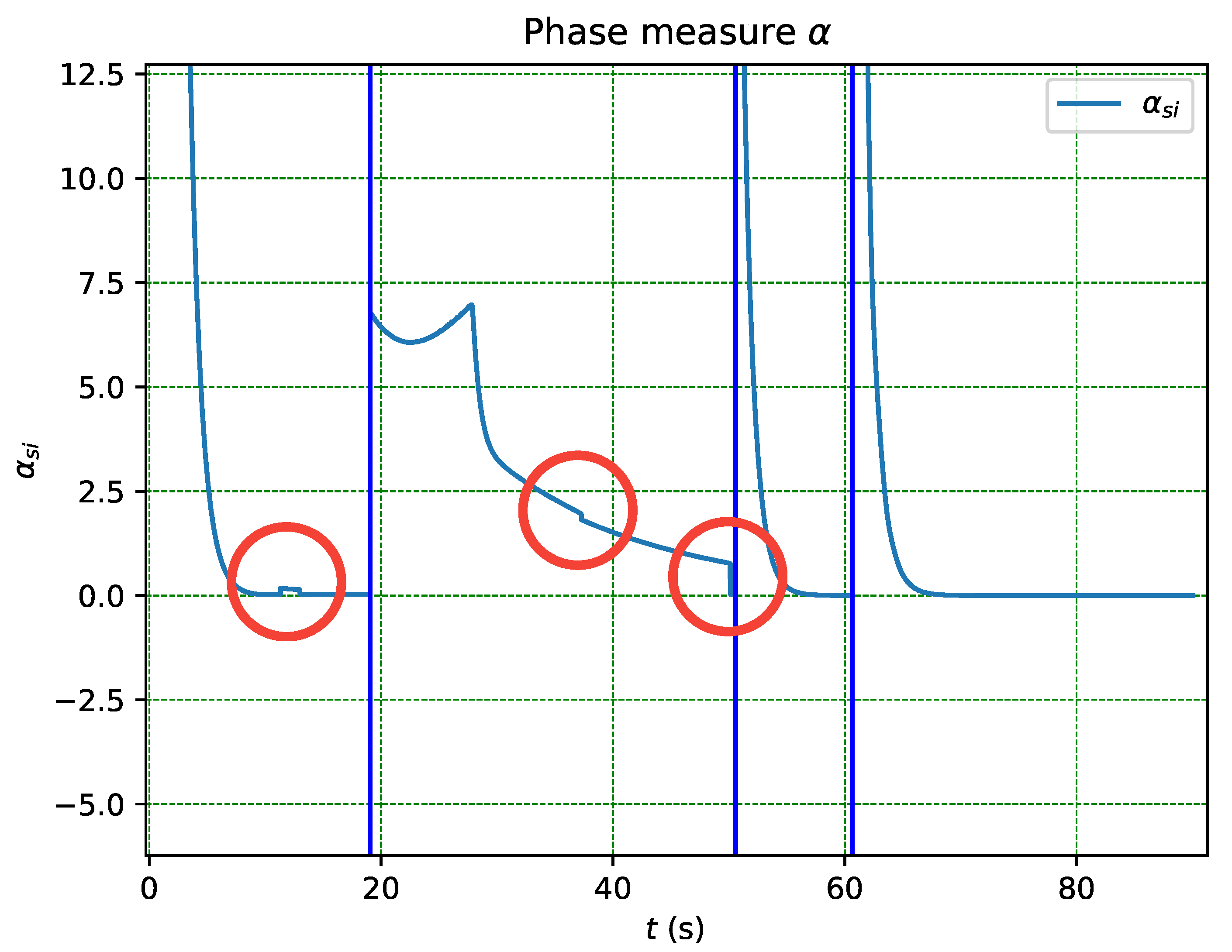
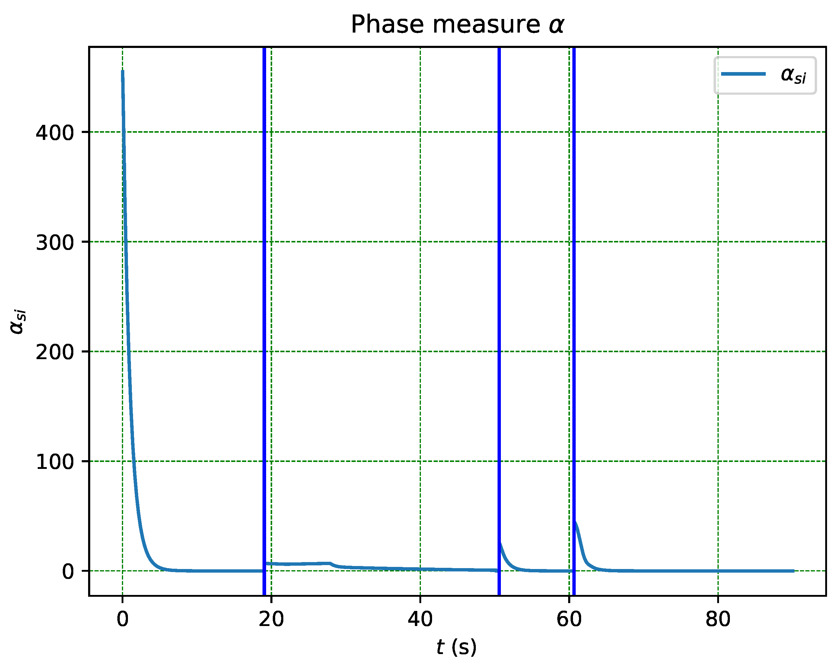
The function
, defined in (
35) and based on the error within phase
, serves as the applied measure. The system exhibits robustness against uncertainty in
measurement, as evidenced by the recurrent activation of obstacle and collision avoidance tasks in
Figure 14, without immediate transition until the error persists and the transition probability increases. This is in contrast to other schemes where the transition occurs as soon as a flag is crossed, leading to transition even in the presence of false positives arising from uncertainty in sensor measurement.
Figure 14.
Close up of the Measure from
Figure 15.
Figure 14.
Close up of the Measure from
Figure 15.
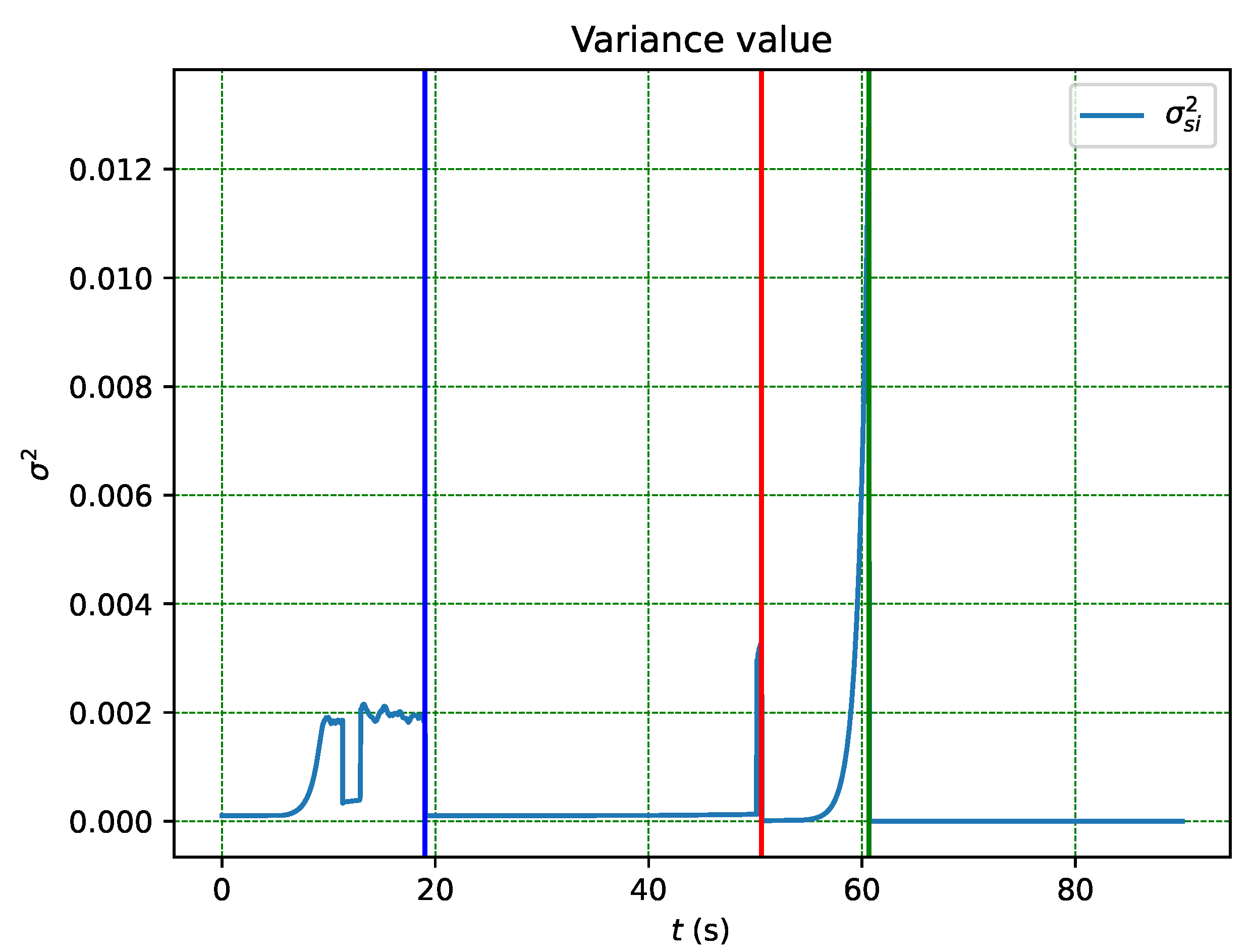
Due to the behaviour of the
distribution in each phase, the variance of each phase starts at zero and tends towards the next state until a transition occurs, as shown in
Figure 16. The variance in a finite-state Markov chain is always bounded since there are a limited number of transitions from the current state. Thus, the validation of Theorem 1 is shown in
Figure 16.
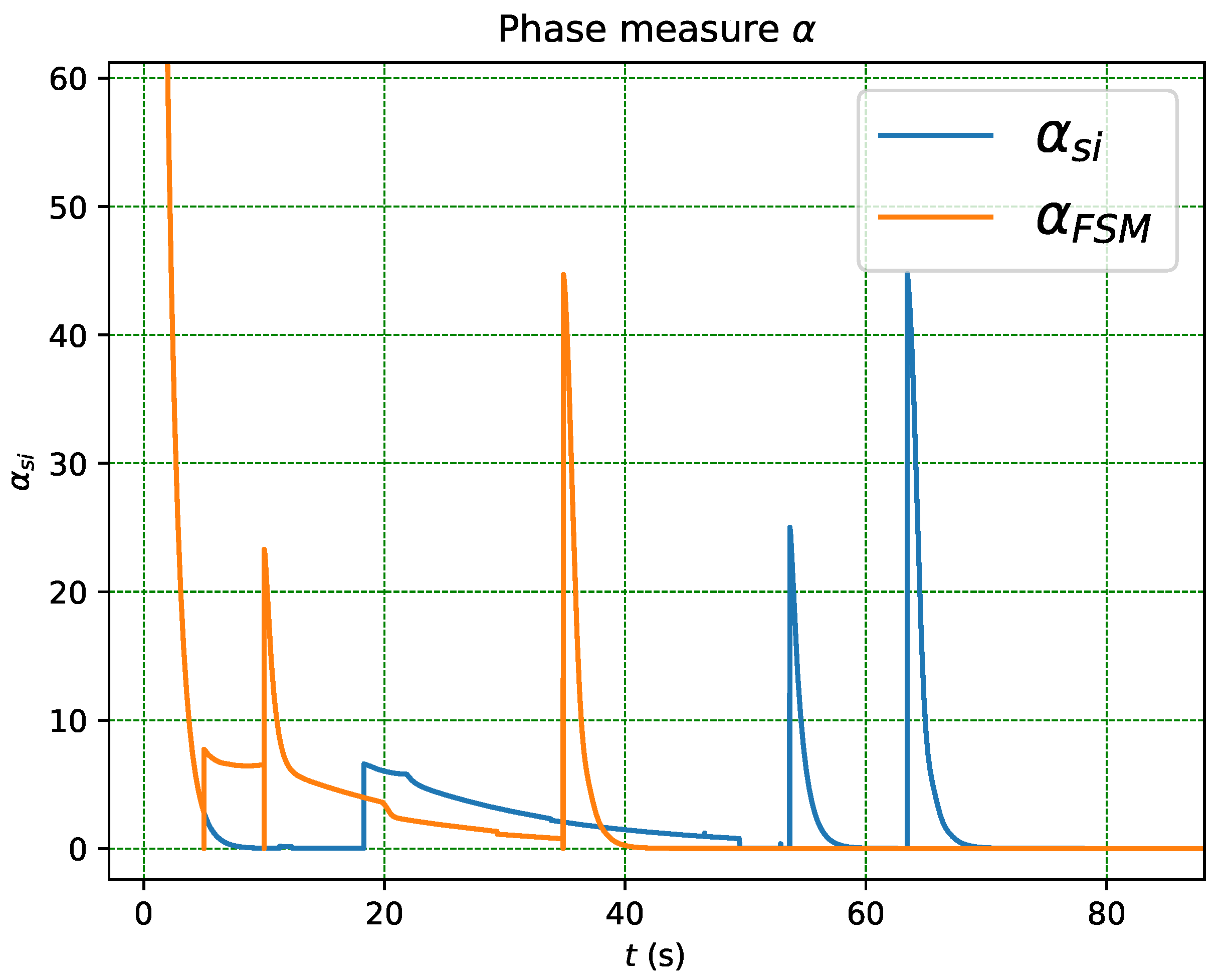
8.6. Comparison of DTMC and FSM in the Presence of Unexpected Failures
Figure 17 compares the DTMC and FSM decision agents for the same manipulation task in the case of unexpected failures that lead to the loss of partial state information and therefore the error in the measure of
of the system. The experience in the use of the system indicates that a flag error limit of
is necessary for the correct functioning of the FSM while DTMC does not need such information. The failures occur between
and
.
The DTMC-based decision agent is able to recover from the failure and continues to make the correct decision, while the FSM-based decision agent is unable to recover and continues to make the incorrect decision. Note that at t = 5, due to the unexpected transition, the FSM decision agent can no longer satisfy the behaviour in the first phase, which implies that the following behaviours can no longer be satisfied. This highlights the advantage of using DTMC-based decision agents, as they are more robust and can handle unexpected failures better than FSM-based agents.


