
Integrated Optimization Model for Maintenance Policies and Quality Control Parameters for Multi-Component System
 , , , , ,
Abstract
:1. Introduction
2. Problem Description
- -
- Type 1 () is related to the mechanical failure of the machines in the system.
- -
- Type 2 () is quality-related and is observed when the production process goes into an out-of-control state. When such failures are observed, an immediate shutdown occurs, and all corrective actions are carried out to restore the process to its normal operation (i.e., the in-control state). However, the process may also worsen due to external causes, such as operator mistakes, bad quality parts, environmental effects, etc. In this case, the process is reset to the in-control state.
- -
- Each automatic machine can process only one part at a time, which imposes a single characteristic to quality (CTQ).
- -
- Failure modes ( and ) are independent. Failure reports from the company’s records were used to obtain these probabilities.
- -
- The required resources to detect, maintain and restore the process are always available, so no waiting times are considered.
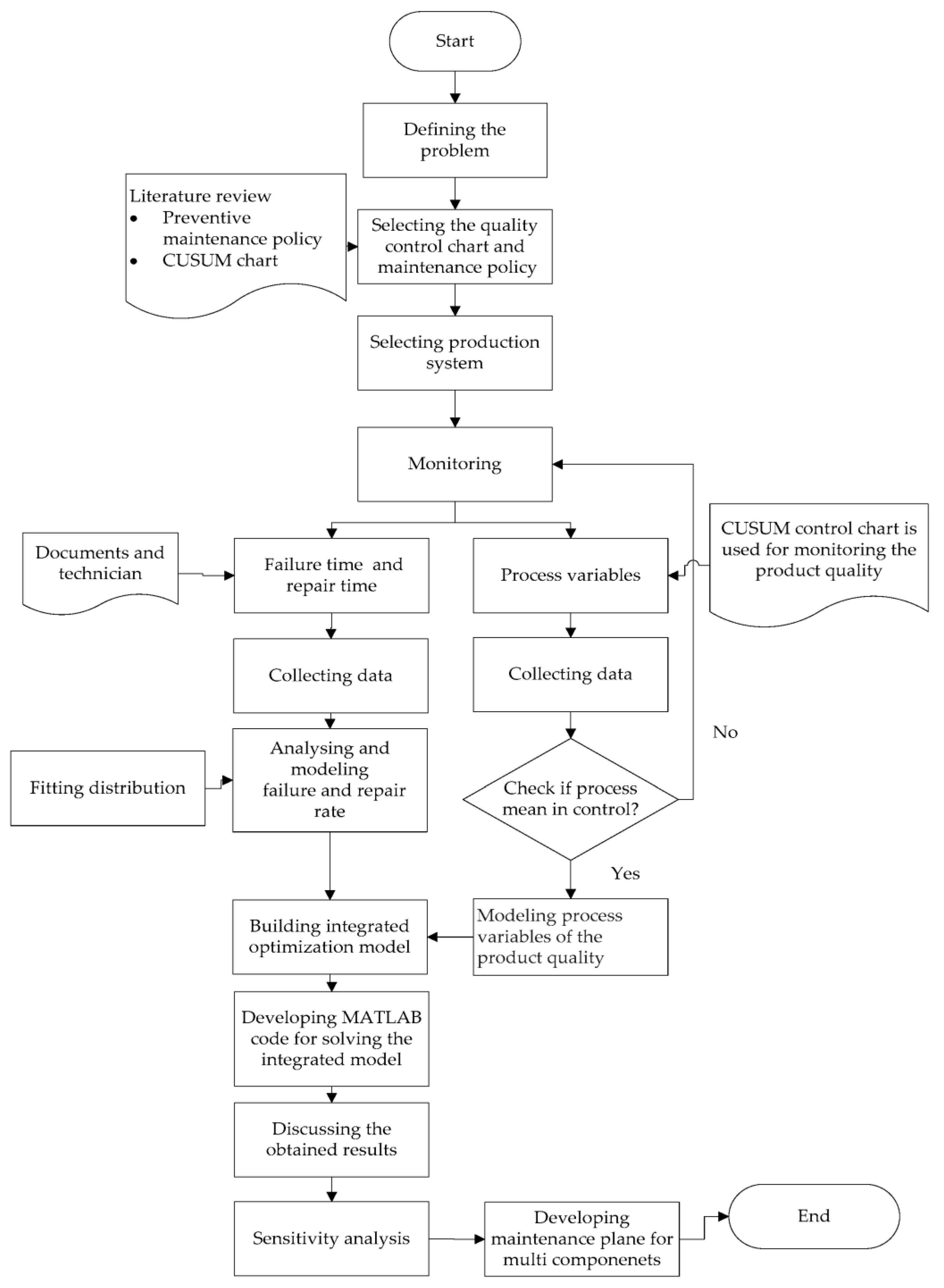
3. Proposed Integrated Optimization Model
- -
- Step 1: Defining the problem. The performance of the manufacturing system is significantly impacted by the breakdown of machines with multi-component.
- -
- Step 2: Select the quality control chart and maintenance policy to develop the model.
- -
- Step 3: Select the production system.
- -
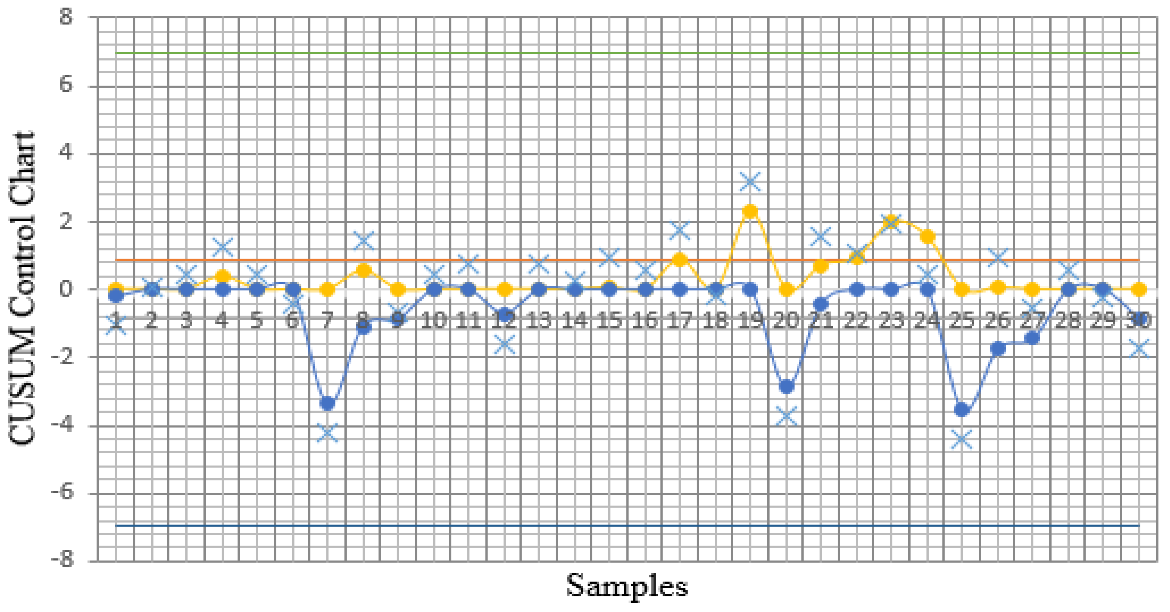
- Step 4: Monitor the selected machine with multi-component using a CUSUM chart.
- -
- Step 5: Monitor the failure and repair rate. In this step, the data related to the mean time between failure and the mean time to repair all selected components were gathered and fitted for suitable distributions.
- -
- Step 6: Develop the integrated model based on CM, PM intervals, and CUSUM chart parameters.
- -
- Step 7: Solve the developed integrated maintenance policy and quality control mathematical model.
- -
- Step 8: Sensitivity analyses were conducted to illustrate the robustness of the developed model due to the stochastic nature of the problem under investigation.
- -
- Step 9: Discuss the obtained results.
- : the expected cost of false alarms, which includes the cost of both investigating and analyzing the false alarms, and it is given as
- : the expected sampling cost per cycle, which can be calculated as follows [45]:
- : the quality loss per unit of time in the control state, which is calculated using the Taguchi loss function (TLF), and is given as [45]
- : the quality loss per unit time when the process is in an out-of-control state due to machine degradation, which is also calculated using the Taguchi loss function (TLF) and is given as [45]
- : the quality loss per unit of time when the process is in an out-of-control state due to external factors (), which is also calculated using the Taguchi loss function (TLF) and is given as [45]
- : the expected cost of detecting and repairing the process due to external causes ().
- : the expected cost of resetting and restoring the process (through CM) after a downtime of Type 2 (), which is calculated as follows:
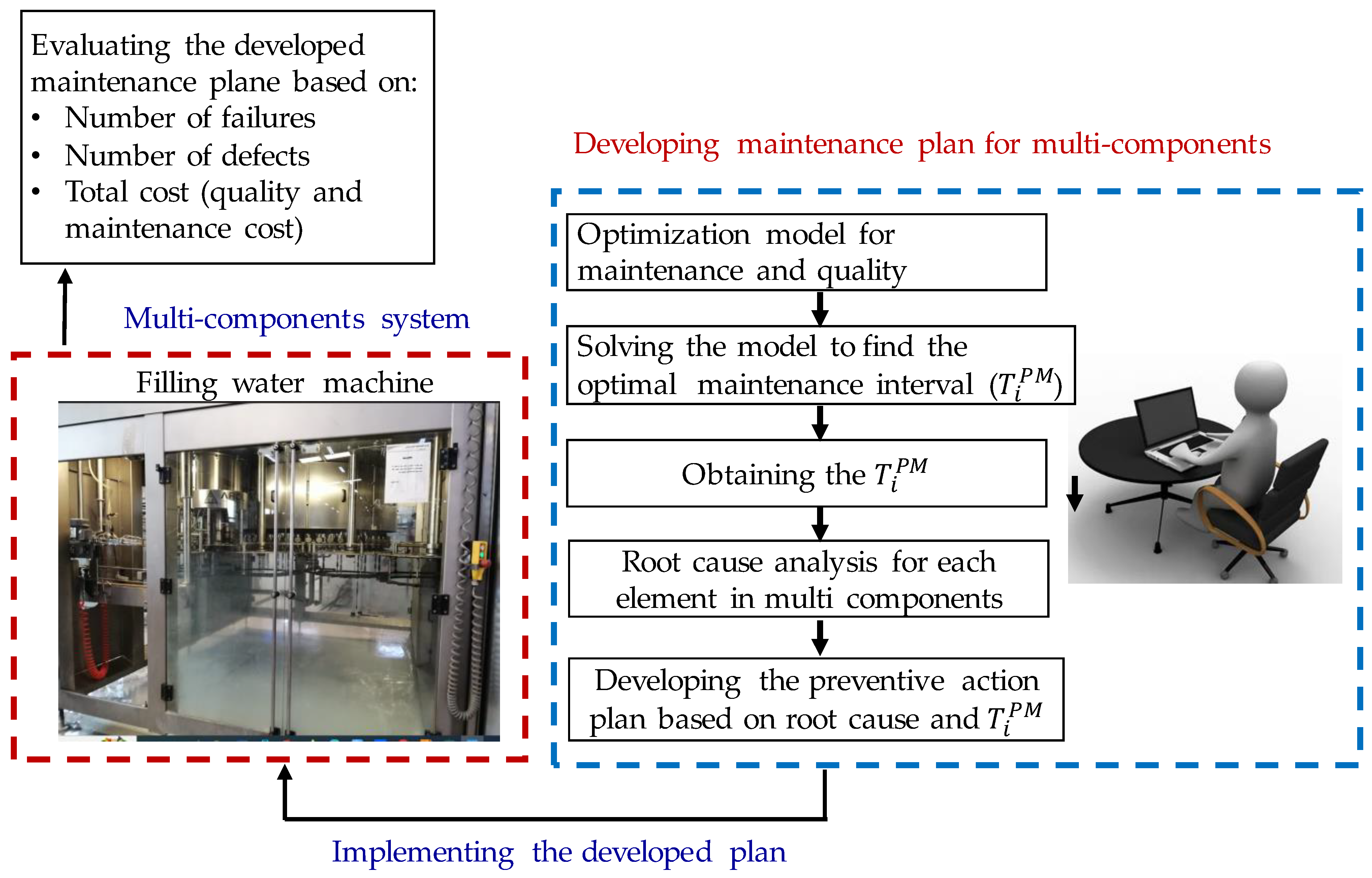
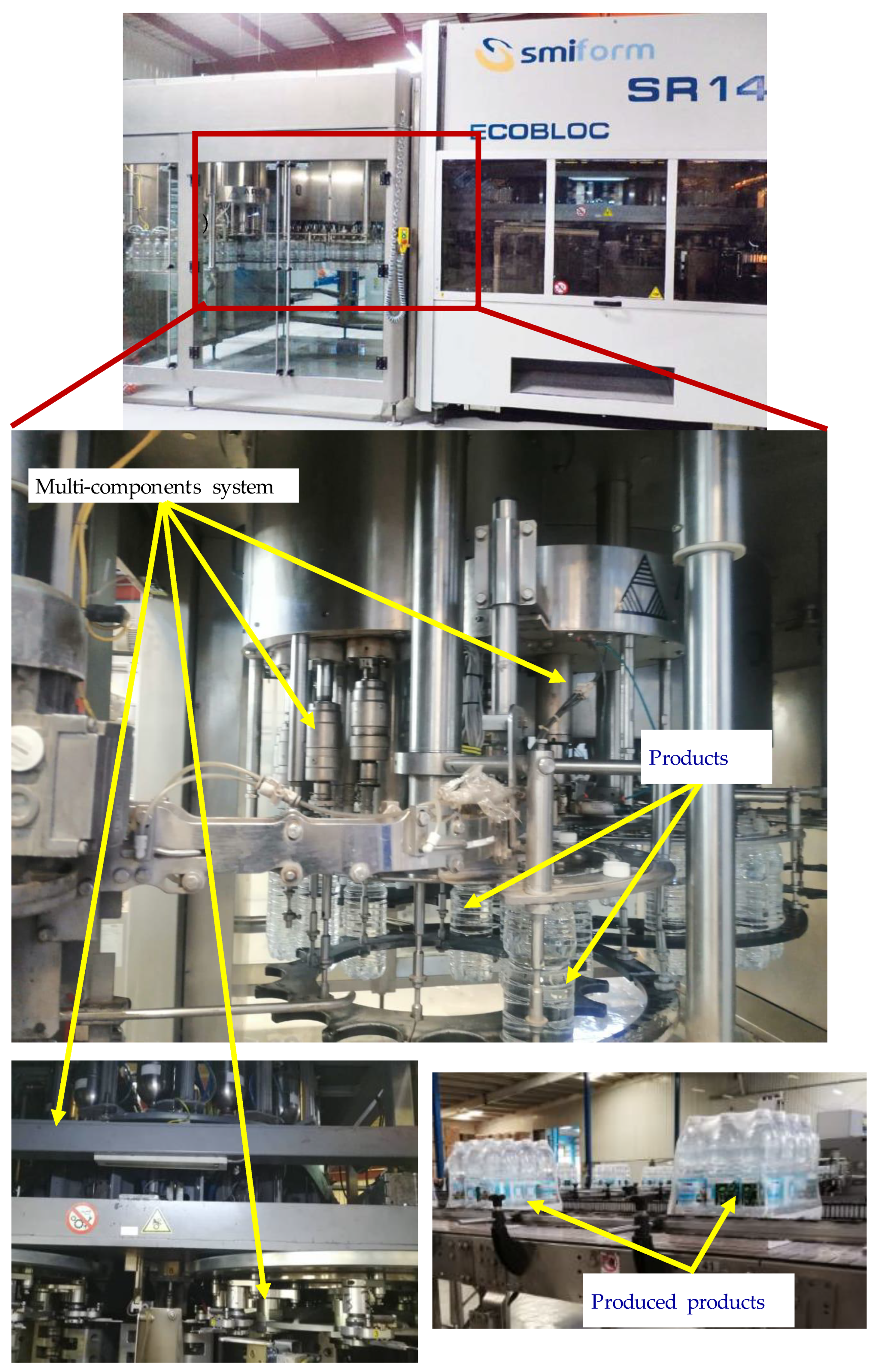
4. Case Study
5. Results
5.1. Design of Experiments Based on One-Factor-at-a-Time
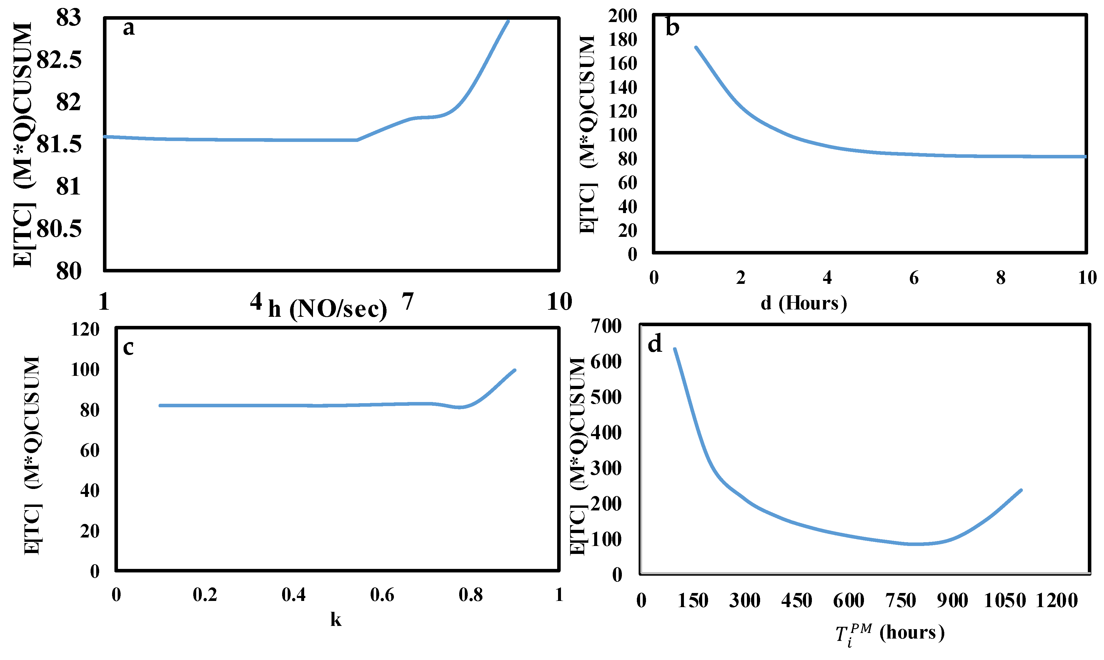
5.2. Sensitivity Analysis
5.3. Preventive Actions to Reduce the Defects
6. Conclusions
- -
- Managers can control the quality of produced units and monitor the production line and its different states using the proposed solution steps.
- -
- The proposed methodology helps to identify the optimal preventive maintenance interval needed to improve production output and minimize downtime with enhanced product quality.
- -
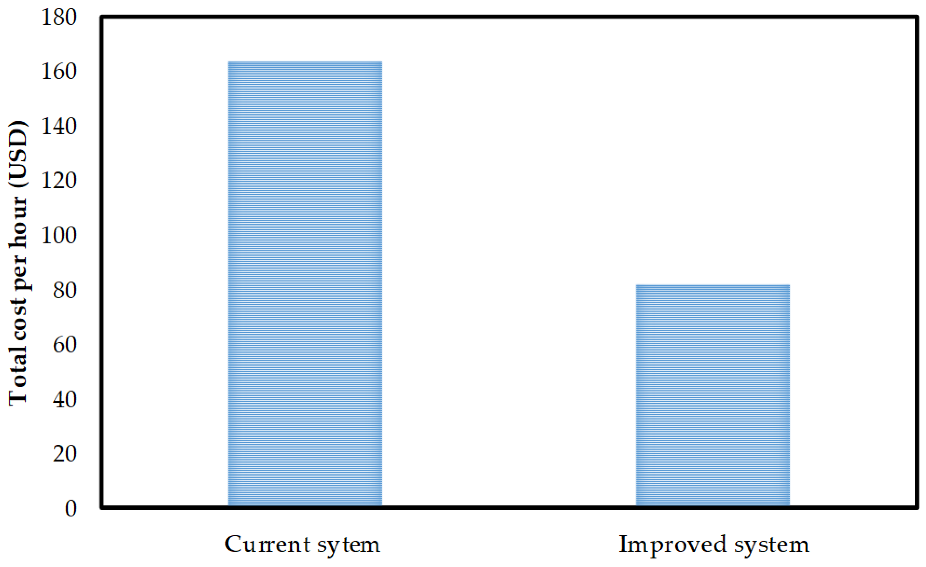
- A maintenance plan for a multi-component system was developed based on the optimal value of preventive maintenance interval. The result showed that the total cost was reduced by approximately 50% compared with the current system.
Author Contributions
Funding
Data Availability Statement
Acknowledgments
Conflicts of Interest
List of Abbreviations
| Notation | Descriptions | |
| Decision variables | ||
| h | Sample frequency (average number of samples obtained in one second (NO/second) | |
| d | Decision Interval (hours) | |
| k | Coefficient of control limit | |
| n | Sample size | |
| Preventive maintenance interval (hours) | ||
| Parameters | ||
| CTQ | Critical to quality characteristic | |
| The normal density function of quality characteristic (∎) | ||
| Number of corrective maintenance actions | ||
| Number of preventive maintenance actions | ||
| Quality loss per unit time in the control state (USD) | ||
| Quality loss per unit of time due to machine degradation (USD) | ||
| Quality loss per unit of time due to external factors () (USD) | ||
| Number of components | ||
| Number of preventive maintenance for ith component | ||
| P | Production rate (Carton/hour) | |
| S | Expected number of samples while the process is in-control | |
| The proportion of non-conforming units when the process is in-control state | ||
| Probability of non-conforming items produced due to machine failure | ||
| Probability of non-conforming items produced due to external factors | ||
| δ | Magnitude of shift | |
| μ0 | Target value (mm) | |
| σ0 | Standard deviation | |
| λ | Process failure rate | |
| λ1 | Failure rate due to an external factor | |
| λ2 | Failure rate due to machine degradation | |
| αi | The shape parameter of Weibull distribution for ith component | |
| γi | Scale parameter of Weibull distribution for ith component | |
| Δ | Tolerance factor | |
| Cost parameters | ||
| A | Scrap or rework cost (USD) | |
| Corrective maintenance cost (USD) | ||
| Preventive maintenance cost (USD) | ||
| Cost of process quality loss () (USD) | ||
| The expected cost of process quality (USD) | ||
| The expected cost of false alarms (USD) | ||
| Expected sampling cost per cycle (USD) | ||
| The expected cost of detecting and repairing the process due to external factors () (USD) | ||
| The expected cost of resetting and restoring the process (through CM) after a downtime of Type 2 (USD) | ||
| Cf | Cost of investigating a false alarm per unit of time (USD) | |
| Cost of resetting (USD) | ||
| The expected cost of preventive maintenance (PM) (USD) | ||
| The expected total cost of quality loss due to process failure | ||
| Expected total cost per unit of time (USD/hour) | ||
| F | Fixed cost of the sample (USD) | |
| Fixed cost for corrective maintenance (USD) | ||
| Fixed cost of corrective maintenance of ith component (USD) | ||
| Fixed cost of preventing maintenance of ith component(USD) | ||
| The labor cost (USD/hour) | ||
| Cost of production lost (USD/hour) | ||
| V | The variable cost of the sample | |
| Statistical properties parameters | ||
| Average run length in-control state (average number of samples taken before a false alarm occurs) | ||
| ARL1 | Average run length in an out-of-control state | |
| Average run length due to external factors | ||
| Average run length due to machine failure | ||
| Time parameters | ||
| Repair times required to perform corrective maintenance (hours) | ||
| Repair times required to perform preventive maintenance (hours) | ||
| MTF | Mean time between process failure (hours) | |
| An estimate of the time it takes to determine if assignable causes have occurred (hours) | ||
| Cycle time (hours) | ||
| te | Time evaluation period (hours) | |
| tf | False alarm search time (hours) | |
| tr | Expected time to reset the process (hours) | |
| Time required for corrective maintenance of ith component (hours) | ||
| Time required for preventive maintenance of ith component (hours) | ||
| ts | Time for the sample and plot a chart (hours) | |
References
- He, Y.; Gu, C.; Chen, Z.; Han, X. Integrated Predictive Maintenance Strategy for Manufacturing Systems by Combining Quality Control and Mission Reliability Analysis. Int. J. Prod. Res. 2017, 55, 5841–5862. [Google Scholar] [CrossRef]
- Esmaeili, E.; Karimian, H.; Najjartabar, M. Analyzing the Productivity of Maintenance Systems Using System Dynamics Modeling Method. Int. J. Syst. Assur. Eng. Manag. 2018, 10, 201–211. [Google Scholar] [CrossRef]
- Pei, Y.; Liu, Z.; Xu, J.; Qi, B.; Cheng, Q. Grouping Preventive Maintenance Strategy of Flexible Manufacturing Systems and Its Optimization Based on Reliability and Cost. Machines 2023, 11, 74. [Google Scholar] [CrossRef]
- Mishra, A.K.; Shrivastava, D.; Vrat, P. An Opportunistic Group Maintenance Model for the Multi-Unit Series System Employing Jaya Algorithm. Opsearch 2020, 57, 603–628. [Google Scholar] [CrossRef]
- Azadeh, A.; Abdolhossein Zadeh, S. An Integrated Fuzzy Analytic Hierarchy Process and Fuzzy Multiple-Criteria Decision-Making Simulation Approach for Maintenance Policy Selection. Simulation 2016, 92, 3–18. [Google Scholar] [CrossRef]
- Dao, C.D.; Zuo, M.J. Selective Maintenance of Multi-State Systems with Structural Dependence. Reliab. Eng. Syst. Saf. 2017, 159, 184–195. [Google Scholar] [CrossRef]
- Laggoune, R.; Chateauneuf, A.; Aissani, D. Preventive Maintenance Scheduling for a Multi-Component System with Non-Negligible Replacement Time. Int. J. Syst. Sci. 2010, 41, 747–761. [Google Scholar] [CrossRef]
- Shi, H.; Zeng, J. Real-Time Prediction of Remaining Useful Life and Preventive Opportunistic Maintenance Strategy for Multi-Component Systems Considering Stochastic Dependence. Comput. Ind. Eng. 2016, 93, 192–204. [Google Scholar] [CrossRef]
- Shaheen, B.W.; Németh, I. Integration of Maintenance Management System Functions with Industry 4.0 Technologies and Features—A Review. Processes 2022, 10, 2173. [Google Scholar] [CrossRef]
- Wang, K.; Deng, C.; Ding, L. Optimal Condition-Based Maintenance Strategy for Multi-Component Systems under Degradation Failures. Energies 2020, 13, 4346. [Google Scholar] [CrossRef]
- Dekker, R.; Roelvink, I.F.K. Marginal Cost Criteria for Preventive Replacement of a Group of Components. Eur. J. Oper. Res. 1995, 84, 467–480. [Google Scholar] [CrossRef] [Green Version]
- Huang, J. A Heuristic Replacement Scheduling Approach for Multi-Unit Systems with Economic Dependency. Int. J. Reliab. Qual. Saf. Eng. 1996, 3, 1–10. [Google Scholar] [CrossRef]
- Samrout, M.; Yalaoui, F.; Châtelet, E.; Chebbo, N. New Methods to Minimize the Preventive Maintenance Cost of Series-Parallel Systems Using Ant Colony Optimization. Reliab. Eng. Syst. Saf. 2005, 89, 346–354. [Google Scholar] [CrossRef]
- Laggoune, R.; Chateauneuf, A.; Aissani, D. Opportunistic Policy for Optimal Preventive Maintenance of a Multi-Component System in Continuous Operating Units. Comput. Chem. Eng. 2009, 33, 1499–1510. [Google Scholar] [CrossRef]
- Rivera-Gómez, H.; Gharbi, A.; Kenné, J.P.; Montaño-Arango, O.; Corona-Armenta, J.R. Joint Optimization of Production and Maintenance Strategies Considering a Dynamic Sampling Strategy for a Deteriorating System. Comput. Ind. Eng. 2020, 140, 106273. [Google Scholar] [CrossRef]
- Magnanini, M.C.; Tolio, T. Switching- and Hedging- Point Policy for Preventive Maintenance with Degrading Machines: Application to a Two-Machine Line. Flex. Serv. Manuf. J. 2020, 32, 241–271. [Google Scholar] [CrossRef] [Green Version]
- Kuhnle, A.; Jakubik, J.; Lanza, G. Reinforcement Learning for Opportunistic Maintenance Optimization. Prod. Eng. 2019, 13, 33–41. [Google Scholar] [CrossRef]
- Zhou, W.H.; Zhu, G.L. Economic Design of Integrated Model of Control Chart and Maintenance Management. Math. Comput. Model. 2008, 47, 1389–1395. [Google Scholar] [CrossRef]
- Cheng, G.; Li, L. Joint Optimization of Production, Quality Control and Maintenance for Serial- Parallel Multistage Production Systems. Reliab. Eng. Syst. Saf. 2020, 204, 107146. [Google Scholar] [CrossRef]
- Duffuaa, S.; Kolus, A.; Al-Turki, U.; El-Khalifa, A. An Integrated Model of Production Scheduling, Maintenance and Quality for a Single Machine. Comput. Ind. Eng. 2020, 142, 106239. [Google Scholar] [CrossRef]
- Salmasnia, A.; Abdzadeh, B.; Namdar, M. A Joint Design of Production Run Length, Maintenance Policy and Control Chart with Multiple Assignable Causes. J. Manuf. Syst. 2017, 42, 44–56. [Google Scholar] [CrossRef]
- Salmasnia, A.; Soltani, F.; Heydari, E.; Googoonani, S. An Integrated Model for Joint Determination of Production Run Length, Adaptive Control Chart Parameters and Maintenance Policy. J. Ind. Prod. Eng. 2019, 36, 401–417. [Google Scholar] [CrossRef]
- Fath, B.D.; Bizon, N.; Yang, L.; Liu, Q.; Xia, T.; Ye, C.; Li, J. Preventive Maintenance Strategy Optimization in Manufacturing System Considering Energy Efficiency and Quality Cost. Energies 2022, 15, 8237. [Google Scholar] [CrossRef]
- Ben-Daya, M. Integrated Production Maintenance and Quality Model for Imperfect Processes. IIE Trans. (Institute Ind. Eng.) 1999, 31, 491–501. [Google Scholar] [CrossRef]
- Rahim, M.A. Economic Design of X Control Charts Assuming Weibull In-Control Times. J. Qual. Technol. 1993, 25, 296–305. [Google Scholar] [CrossRef]
- Lee, B.H.; Rahim, M.A. An Integrated Economic Design Model for Quality Control, Replacement, and Maintenance. Qual. Eng. 2001, 13, 581–593. [Google Scholar] [CrossRef]
- Hajej, Z.; Nyoungue, A.C.; Abubakar, A.S.; Mohamed Ali, K. An Integrated Model of Production, Maintenance, and Quality Control with Statistical Process Control Chart of a Supply Chain. Appl. Sci. 2021, 11, 4192. [Google Scholar] [CrossRef]
- Baker, K.R. Two Process Models in the Economic Design of an x Chart. AIIE Trans. 1971, 3, 257–263. [Google Scholar] [CrossRef]
- Montgomery, D.C.; Heikes, R.G. Process Failure Mechanisms and Optimal Design of Fraction Defective Control Charts. AIIE Trans. 1976, 8, 449–455. [Google Scholar] [CrossRef]
- Lorenzen, T.J.; Vance, L.C. The Economic Design of Control Charts: A Unified Approach. Technometrics 1986, 28, 3. [Google Scholar] [CrossRef]
- Haq, A.; Awais, M. New Shewhart-EWMA and Shewhart-CUSUM Control Charts for Monitoring Process Mean. Sci. Iran. 2018, 26, 3796–3818. [Google Scholar] [CrossRef] [Green Version]
- Moskowitz, H.; Plante, R.; Chun, Y.H. Effect of Process Failure Mechanisms on Economic X Control Charts. IIE Trans. (Inst. Ind. Eng.) 1994, 26, 12–21. [Google Scholar] [CrossRef]
- Liew, J.Y.; Khoo, M.B.C.; Neoh, S.G. A Study on the Effects of a Skewed Distribution on the EWMA and MA Charts. AIP Conf. Proc. 2014, 1605, 1034–1039. [Google Scholar] [CrossRef]
- Sultana, I.; Ahmed, I.; Azeem, A.; Sarker, N.R. Economic Design of Exponentially Weighted Moving Average Chart with Variable Sampling Interval at Fixed Times Scheme Incorporating Taguchi Loss Function. Int. J. Ind. Syst. Eng. 2018, 29, 428–452. [Google Scholar] [CrossRef]
- De Vargas, V.D.C.C.; Lopes, L.F.D.; Souza, A.M. Comparative Study of the Performance of the CuSum and EWMA Control Charts. Comput. Ind. Eng. 2004, 46, 707–724. [Google Scholar] [CrossRef]
- Shrivastava, D.; Kulkarni, M.S.; Vrat, P. Integrated Design of Preventive Maintenance and Quality Control Policy Parameters with CUSUM Chart. Int. J. Adv. Manuf. Technol. 2016, 82, 2101–2112. [Google Scholar] [CrossRef]
- Li, Y.; Chen, Z.; Pan, E. Joint Economic Design of CUSUM Control Chart and Age-Based Imperfect Preventive Maintenance Policy. Math. Probl. Eng. 2018, 2018, 9246372. [Google Scholar] [CrossRef] [Green Version]
- Saha, R. Integrated Economic Design of Quality Control and Maintenance Management Using CUSUM Chart with VSIFT Sampling Policy. Master’s Thesis, Bangladesh University of Engineering and Technology, Dhaka, Bangladesh, 2017. [Google Scholar]
- Farahani, A.; Tohidi, H.; Shoja, A. An Integrated Optimization of Quality Control Chart Parameters and Preventive Maintenance Using Markov Chain. Adv. Prod. Eng. Manag. 2019, 14, 5–14. [Google Scholar] [CrossRef] [Green Version]
- Al-Shayea, A.; Noman, M.A.; Nasr, E.A.; Kaid, H.; Kamrani, A.K.; El-Tamimi, A.M. New Integrated Model for Maintenance Planning and Quality Control Policy for Multi-Component System Using an EWMA Chart. IEEE Access 2019, 7, 160623–160636. [Google Scholar] [CrossRef]
- Pandey, D.; Kulkarni, M.S.; Vrat, P. A Methodology for Simultaneous Optimisation of Design Parameters for the Preventive Maintenance and Quality Policy Incorporating Taguchi Loss Function. Int. J. Prod. Res. 2012, 50, 2030–2045. [Google Scholar] [CrossRef]
- Kamal, M.M.; Arumugam, S.; Yousuf, M. Importance of Maintenance in the Context of Multicomponent Systems. J. Qual. Maint. Eng. 2015, 4, 433–448. [Google Scholar]
- Page, E.S. Control Charts for the Mean of a Normal Population. J. R. Stat. Soc. Ser. B 1954, 16, 131–135. [Google Scholar] [CrossRef]
- Cassady, C.R.; Kutanoglu, E. Integrating Preventive Maintenance Planning and Production Scheduling for a Single Machine. IEEE Trans. Reliab. 2005, 54, 304–309. [Google Scholar] [CrossRef]
- Pandey, D.; Kulkarni, M.S.; Vrat, P. A Methodology for Joint Optimization for Maintenance Planning, Process Quality and Production Scheduling. Comput. Ind. Eng. 2011, 61, 1098–1106. [Google Scholar] [CrossRef]


| (Ni) | Components | Number | Shape Parameter αi | Scale Parameter γi (hr) | Component Cost during Replacement (USD) | Sub-Component/Consumable Cost through Repair (USD) | TRCMi (h) | TRPMi (h) |
|---|---|---|---|---|---|---|---|---|
| 1 | Filling Head | 54 | 19,440 (USD 360/pc) | - | - | - | ||
| Seals and O-rings for filling heads | 108 set | 3.7761 | 1294.3 | 8700 (USD 80.55/pc) | 90 | 2 | 4 | |
| 2 | Flowmeter | 54 | 1.4934 | 4426.8 | 162,000 (USD 3000/pc) | n/a | 1.25 | n/a |
| 3 | Valve Battery | 14 | 1.7101 | 3745.1 | 14,000 (USD 1000/pc) | 350 | 1 | 9 |
| 4 | Fill box Flux | 27 | 1.3329 | 4768.7 | 26,490 (USD 981/pc) | n/a | 1.5 | n/a |
| Parameter | Value | Parameter | Value |
|---|---|---|---|
| (cartons/h) | 600 | (USD/bottle) | 0.016 |
| (h) | 0.33 | (USD/bottle) | 0.036 |
| (h) | 0.5 | 0.138 | |
| (h) | 0.5 | 9.2 | |
| (h) | 0.25 | 9 | |
| (USD)/h | 10 | Δ | 3 |
| USD/h | 8 | A USD/bottle | 0.069 |
| 1 | 0.8 |
| Variables | Optimal Value |
|---|---|
| n | 1 |
| d | ≃10 |
| h | 5 |
| k | 0.10166 |
| 800 | |
| E[TC](M∗Q) CUSUM | 81.5479 |
| Decision Variables | Ranges |
|---|---|
| n | 1 |
| d | 8–≃10 |
| h | 4–5 |
| k | 0.10166 |
| 750–850 |
| Parameter | Basic Level 1 | Level 2 (+10%) | Level 3 (+20%) | E[CT](M∗Q)CUSUM | |||
|---|---|---|---|---|---|---|---|
| Basic Level | Level 2 | Level 3 | Range | ||||
| ts | 0.33 | 0.363 | 0.396 | 81.5479 | 81.5479 | 81.5479 | 81.5479 |
| tf | 0.5 | 0.55 | 0.6 | 81.5479 | 81.5479 | 81.5479 | 81.5479 |
| ta | 0.5 | 0.55 | 0.6 | 81.5479 | 81.5479 | 81.5479 | 81.5479 |
| tr | 0.25 | 0.275 | 0.3 | 81.5479 | 81.5479 | 81.5479 | 81.5479 |
| A | 0.069 | 0.0759 | 0.0828 | 81.5479 | 81.5479 | 81.5479 | 81.5479 |
| F | 0.016 | 0.176 | 0.0192 | 81.5479 | 81.5479 | 81.5479 | 81.5479 |
| V | 0.036 | 0.0396 | 0.0432 | 81.5479 | 81.5479 | 81.5479 | 81.5479 |
| Cr | 0.138 | 0.1518 | 0.1656 | 81.5479 | 81.5479 | 81.5479 | 81.5479 |
| Cf | 9.2 | 10.12 | 11.04 | 81.5479 | 81.5479 | 81.5479 | 81.5479 |
| Cs | 9 | 9.9 | 10.8 | 81.5479 | 81.5479 | 81.5479 | 81.5479 |
| Lp | 8 | 8.8 | 9.6 | 81.5479 | 89.6698 | 97.7117 | 81.5479–97.7117 |
| L | 10 | 10.10 | 12 | 81.5479 | 81.5496 | 81.5815 | 81.5479–81.5815 |
| No. | Components | |
|---|---|---|
| 1 | Seals and O-rings for filling heads | |
| Problem | Leakage in water | |
| Root causes | Replace the Seals and O-rings | |
| Solution | Periodically replace the O-rings | |
| 2 | Flowmeter | |
| Problem | Water not flowing or continually flows | |
| Root causes | Malfunction with the internal electronic card | |
| Solution | Replace the flowmeter | |
| 3 | Valve Battery | |
| Problem | Water not flowing according to the set level | |
| Root causes | The presence of an air leak from the O-rings | |
| An issue with the electronic card of the valve battery | ||
| An issue in the inner Spring of the valve | ||
| Solution | Change the O-rings of the valve battery or change the card. | |
| Change the inner springs of the valve battery | ||
| 4 | Fillbox Flux | |
| Problem | The filling cycle is not initiated, or filling heads are not working | |
| Root causes | An issue with the motherboard. | |
| The problem with the data cable | ||
| The problem with the control system | ||
| Solution | Check the electronic card for repair or replacement if available otherwise, replace it with a new Fillbox | |
| Repair the cable data or replace | ||
| Reinstall the program for the Fill box to reset the system | ||
Disclaimer/Publisher’s Note: The statements, opinions and data contained in all publications are solely those of the individual author(s) and contributor(s) and not of MDPI and/or the editor(s). MDPI and/or the editor(s) disclaim responsibility for any injury to people or property resulting from any ideas, methods, instructions or products referred to in the content. |
© 2023 by the authors. Licensee MDPI, Basel, Switzerland. This article is an open access article distributed under the terms and conditions of the Creative Commons Attribution (CC BY) license (https://creativecommons.org/licenses/by/4.0/).
Share and Cite
Nasr, M.M.; Naji, F.; Amrani, M.; Ghaleb, M.; Alqahtani, K.N.; Othman, A.M.; Abualsauod, E.H. Integrated Optimization Model for Maintenance Policies and Quality Control Parameters for Multi-Component System. Machines 2023, 11, 435. https://doi.org/10.3390/machines11040435
Nasr MM, Naji F, Amrani M, Ghaleb M, Alqahtani KN, Othman AM, Abualsauod EH. Integrated Optimization Model for Maintenance Policies and Quality Control Parameters for Multi-Component System. Machines. 2023; 11(4):435. https://doi.org/10.3390/machines11040435
Chicago/Turabian StyleNasr, Mustafa M., Fadia Naji, Mokhtar Amrani, Mageed Ghaleb, Khaled N. Alqahtani, Asem Majed Othman, and Emad Hashiem Abualsauod. 2023. "Integrated Optimization Model for Maintenance Policies and Quality Control Parameters for Multi-Component System" Machines 11, no. 4: 435. https://doi.org/10.3390/machines11040435