Boundary Scenario Generation for HAVs Based on Classification and Local Sampling

Abstract

High-level Automated Vehicles (HAVs) are expected to improve traffic safety significantly. However, verifying and evaluating HAVs remains an open problem. Scenario-based testing is a promising method for HAV testing. Boundary scenarios exist around the performance boundary between critical and non-critical scenarios. Testing HAVs in these boundary scenarios is crucial to investigate why collisions cannot be avoided due to small changes in scenario parameters. This study proposes a methodology to generate diverse boundary scenarios to test HAVs. First, an approach is proposed to obtain at least one High-Performance Classifier (HPC) based on two classification algorithms that iteratively guide each other to find uncertain scenarios to improve their performance. Then, the HPC is exploited to find candidate scenarios highly likely to be boundary scenarios. To increase the efficiency of candidate scenario generation, a strategy based on local sampling is presented to find more diverse candidate scenarios based on a small number of them. Numerical experiments show that the HPCs acquired by the method proposed in this study can achieve a classification accuracy of 98% and 99% for random car-following and cut-in scenarios, respectively. Moreover, more than 86% of 271,744 candidate cut-in scenarios derived by local sampling are near the performance boundary.

1. Introduction

About 1.3 million people die annually worldwide due to traffic accidents, with 93% of these fatalities occurring in low- and middle-income countries such as China and India [1], despite these countries having only around 60% of the world’s vehicles. Automated vehicles are considered to be effective in reducing traffic accidents. In the past decade, some High-level Automated Vehicles (HAVs) have been designed by high-tech companies, such as Waymo, Tesla, and Baidu [2,3,4]. HAVs need to be thoroughly tested to prove they are safe enough before being accepted by the public, which is pretty challenging. For example, a self-driving vehicle made by Tesla, a leading American automotive company, crashed into a truck due to a flaw in its perception system that relied on deep-learning technologies [5,6]. Factors from two perspectives contribute to the difficulty of testing HAVs. First, integrating artificial-intelligence technologies into HAVs, such as deep-learning technologies, may introduce uncertainties and risks due to their poor interpretability [7]. Moreover, there are theoretically infinite scenarios in natural traffic, including those that are never observed. A study indicates that millions of miles of road testing are required to prove that a self-driving vehicle is safe enough, which is impractical and unaffordable [8].

Scenario-Based Testing (SBT) is a promising method for HAV testing, which validates and evaluates an HAV safety based on its performance in specific scenarios. A scenario is a temporal sequence of scenes, which includes static objects, dynamic objects, and interrelationships between them [9]. Based on the level of abstraction, there are three types of scenarios: function, logical, and concrete [10]. Function scenarios have the highest-level abstraction, in which natural language is exploited to describe scenarios. In logical scenarios, parameter ranges and distributions are used to define scenarios. A concrete value combination of scenario parameters can define a concrete scenario. To describe highway scenarios better, a five-layer model is proposed in [11], which includes road networks, traffic participants, weather, et al. Furthermore, the authors in [12] present a modified six-layer model for urban scenario description.

For convenience, “scenario” refers to a concrete scenario in this study if no specific notation is assigned. There are numerous natural traffic scenarios; most are boring and meaningless for AV testing [13]. For example, working on a well-maintained road with no other vehicles or bad weather conditions poses no challenge to the VUT. Rather, the critical and challenging scenarios are significant for scenario-based testing. In a critical scenario, the Vehicle Under Test (VUT) is responsible for at least one collision or near crash [14]. It is a hot research topic to generate critical scenarios for AV testing.

In [15,16], performance boundaries refer to the ones around which VUT performance varies greatly in two adjacent scenarios. Boundary scenarios are those located near performance boundaries. In this study, the performance boundary in an Operational Designed Domain (ODD) [17] is between the sets of critical and non-critical scenarios, and boundary scenarios are near the performance boundary. It is essential to test Highly Automated Vehicles (HAVs) in boundary scenarios to investigate why even minor changes in scenario parameters may lead to a collision. For example, given a new HAV, it is reasonable and expected that many critical scenarios can be found in its ODD. However, it will consume many resources to execute all critical scenarios in the physical or simulation world. To enhance testing efficiency, it is a good option for developers to investigate the HAV performance in boundary scenarios. Furthermore, based on boundary scenarios, the performance boundary can be fitted, which can assist in generating critical scenarios [16,18]. However, it is challenging to identify a large number of diverse boundary scenarios with limited resources because of their rarity. Theoretically, a scenario should not be identified as a boundary one before being proved near the performance boundary, which often requires the execution of many scenarios. In this study, we aim to efficiently generate numerous and diverse scenarios likely to be boundary scenarios, known as candidate scenarios.

The main contributions of this study are as follows:

(1)

A novel approach is proposed to obtain a High-Performance Classifier (HPC) for efficiently classifying critical and non-critical scenarios without consuming significant resources. This approach combines the Gaussian Process Classification (GPC) and Support Vector Machine (SVM) algorithms, which mutually detect uncertain scenarios and improve each other’s performance iteratively.

(2)

A distance-based method is presented for identifying candidate scenarios using the HPC without executing scenarios. This approach enables the efficient identification of potential boundary scenarios.

(3)

This study also uses local sampling iteratively to generate diverse candidate scenarios based on a small set of them. This approach can be applied to generate high-dimensional candidate scenarios efficiently.

The rest of this paper is organized as follows. In Section 2, we review related works. Section 3 presents the methodology proposed by this study to efficiently generate diverse boundary scenarios without consuming significant computing resources. In Section 4, we describe the detailed settings of the simulation experiments. We provide all numerical results of the simulation experiments and our discussions in Section 5. Finally, we conclude this study in Section 6.

2. Related Works

There are two main methodologies for scenario generation: coverage-oriented and criticality-oriented. Coverage-oriented methods generate diverse scenarios that comprehensively fill the ODD to test AVs. Random sampling [13], mutation testing [19], and combinatorial testing [20] can all be exploited to generate diverse scenarios. However, most scenarios generated by coverage-based methods are not challenging for the VUT, and many scenario executions are required, which demands extensive computing resources. On the other hand, criticality-oriented methods aim to find diverse or the most critical scenarios for HAV testing, reducing unnecessary scenario executions. There are many strategies for critical scenario generation, such as Accelerated Evaluation (AE) [21,22,23,24], search-algorithm-based methods [14,25,26,27,28,29], and Reinforcement Learning-based critical scenario generation [30,31,32,33,34].

AE is first proposed by [21] for HAV testing. First, a large amount of NDD is collected, and the original parameter distribution is fitted. Second, the original distribution is skewed by importance sampling, resulting in an accelerated distribution. Finally, Monte Carlo is used to sample the accelerated distribution, generating scenarios for AV testing. AE can generate more critical scenarios than random sampling and naturalistic scenarios, in which VUT performance can be skewed back to that in natural traffic. Simulation experiments show that AE can generate 200~20,000 times more challenging scenarios than road testing. AE is further improved by reducing the gap between the real parameter distribution and the fitted one, finding the optimal hyperparameters for IS by searching algorithms [21] or the cross-entropy method [24]. However, AE still generates many non-critical scenarios and sometimes requires knowledge about the VUT.

Search algorithms have been applied to solve optimization problems, such as structure optimization [35] and vehicle routing [36]. Guided by a fitness function, search algorithms can iteratively search for the most critical scenarios. Many search algorithms are used to search for critical scenarios, such as Particle Swarm Optimization (PSO) algorithm [26], Genetic Algorithm (GA) [25], and Rapidly exploring Random Tree (RRT) [29]. There are three keys to achieving good results based on search algorithms: designing an appropriate fitness function, balancing exploration and exploitation, and reducing the search space. Different fitness functions usually derive scenarios with varying characteristics [37]. Some criticality metrics are sometimes used as the fitness function, such as Time-To-Collision (TTC) [38] and its variants [39,40,41,42,43]. However, to our knowledge, no signal metric can measure the criticality of all scenarios. It seems an excellent option to combine several scenarios to consider various aspects of the scenario. In [44], a weighted sum of several metrics is used to measure the criticality of a scenario. Although the fitness function design is still open, several templates are provided in [45]. A search algorithm must avoid local optima and find the best global solution to the original problem. In [25], a local fuzzed is applied for exploitation, and GA is exploited for exploration. Simulation experiments show that GA-Fuzzer can find three times more critical cut-in scenarios and consumes fewer computing resources than Reinforce Learning-base Adaptive Stress Testing (RLAST) [33]. However, search algorithm-based methods rely on fitness functions designed by experts. Moreover, a conclusion that the VUT is safe enough cannot be made if no critical scenario is detected because they are all falsification methods.

Reinforcement Learning (RL) is a powerful machine-learning technique and has been used in many fields, such as robot control [46] and graph generation [47]. Like search algorithm-based methods, guided by a pre-defined reward function, challenging scenarios are adaptively generated by RL. In [31], RL identifies critical cut-in scenarios guided by a reward function involving distance headway, TTC, and the required lateral acceleration for collision avoidance. The results of simulation experiments indicate that RLAST can adaptively generate adversarial maneuvers for reference vehicles to disturb the VUT, leading to a 37% increase in the proportion of detected critical scenarios compared to random sampling [33]. Simulation results in [33] show that RLAST is more likely to generate a critical cut-in scenario that makes the VUT fail than Monte Carlo. However, RL-based methods heavily rely on the quality of the pre-defined reward function. Furthermore, similar to search algorithm-based methods, no conclusion about the safety of the VUT can be made if no critical scenario is found. It may take numerous iterations to identify critical scenarios using RL, requiring extensive high-fidelity scenario simulations.

Given the performance boundary which divides the ODD into a critical subspace and a non-critical subspace, all criticality-oriented methods mentioned above can be applied to generate critical scenarios in the critical subspace. A decision tree classifier is used to find the performance boundary in [48], which results in a critical and non-critical subspace. After that, A multi-objective population-based search algorithm is adopted to find critical scenarios in the critical space. Experimental results demonstrate that within 24 h, 731 distinct critical scenarios are generated to evaluate the performance of an Autonomous Emergency Braking (AEB) system.

Performance boundary detection can be broadly categorized into two types of methods: regressor-based and classifier-based. Regressor-based methods leverage high-performance regression models to estimate the performance of the SUT in all scenarios within the ODD, without actually executing each scenario. These methods generally begin by modeling the logical scenario and then use searching techniques, such as adaptive sampling and swarm-based searching, to identify boundary scenarios. Once a diverse set of boundary scenarios is identified, the performance boundary can be derived through fitting or clustering techniques. In [15], a novel approach is presented for detecting performance boundaries between distinct modes. The methodology leverages Gaussian Process Regression (GPR) to construct a Surrogate Model (SM) using a set of random scenarios. Then, adaptive sampling is used to find new and uncertain scenarios based on the variance of the GPR model to improve the GPR-based SM iteratively. With the enhancement of the GPR-based SM, new scenarios tend to be boundary scenarios. Finally, boundaries between different performance modes are identified by density-based clustering. Experiment results demonstrate that the proposed approach successfully identified the boundaries between three performance modes of an uncrewed underwater vehicle. However, it required an extensive computation of 850 thousand scenario executions.

The authors in [49] present a coverage-oriented adaptive sampling strategy to find and execute diverse scenarios involving the VUT. Based on scenario parameters and VUT performance in these executed scenarios, a set of training data is collected and used to train a Multi-Layer Perception (MLP) -based SM. Then, the Descent Searching Approach (DSA) is exploited to search for boundary scenarios based on the MLP-based SM. The results of the simulation experiments show that this methodology is effective in obtaining a high-performance SM and finding boundary scenarios. However, a significant limitation of this methodology is that it still requires many scenario executions to train the high-performance SM. Additionally, the methodology may face challenges in finding boundary scenarios in a high-dimensional Operational Design Domain (ODD).

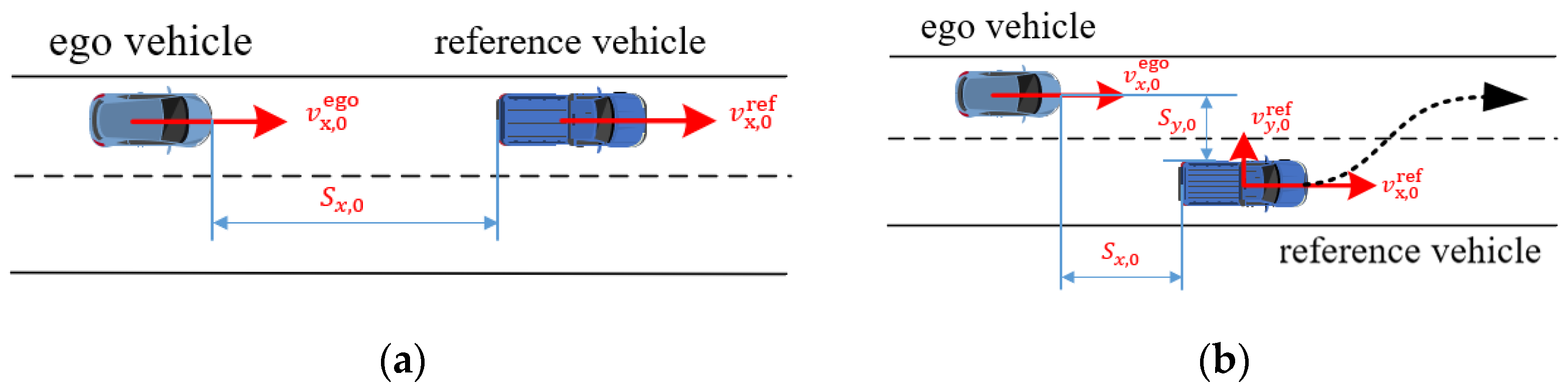
Classifier-based methods find the performance boundary based on an HPC, which classifies all scenarios in the ODD without scenario executions. In [18], Gaussian Process Classification (GPC) is used to find the performance boundary. A GPC model is trained and used to label scenarios in the ODD based on a set of executed scenarios generated by random sampling. The performance boundary is finally estimated, separating the sets of critical and non-critical scenarios. The front-collision-avoidance scenario is described for simulation experiments, involving two vehicles driving on a curved road, the low-speed one (the reference vehicle) and the approaching one (the ego). Three parameters are exploited to describe the scenario: the ego speed, the speed of the reference vehicle, and the aperture angle of the radar sensor of the ego. Numerical results show that less than 1000 random scenarios are sufficient to find the performance boundary. However, this methodology is not compared with other approaches. In addition, As pointed out by the authors of [18], many random scenarios might be needed to train a high-performance GPC model to classify critical and non-critical high-dimensional scenarios, which are resource intensive.

In [50], Gaussian Processes are exploited to distinguish critical and non-critical scenarios. First, a small set of random scenarios is executed to train a GPC model for classifying critical and non-critical scenarios and a GPR model for predicting scenario criticality and uncertainty. Then, a heuristic is adopted to search for critical and uncertain scenarios in the critical space estimated by the GPC model based on the GPR model. After that, the new scenarios are executed and added to the training dataset for GPC and GPR. Simulation experiments involving the scenario described in [18] are carried out to evaluate this methodology. Experiment results show that 56% of the scenarios found by the heuristic algorithm end with a collision. In this methodology, the quality of the new scenarios found by the heuristic algorithm relies on the performance of the GP models. Since the new scenarios tend to be critical and uncertain, the GP model only performs well in a specific critical subspace of the ODD. Therefore, if the initial scenarios for model training are not diverse enough, it is challenging to quickly enhance the performance of the GP models in the whole ODD.

Based on the analysis of the studies mentioned above, it is evident that HPCs or regressors are essential for detecting boundary scenarios. However, it is challenging to obtain these classifiers with limited computing resources. Inspired by [18,49,50], this study presents a methodology to obtain an HPC. GPC and Support Vector Machines (SVM) are employed in this study to classify critical and non-critical scenarios. In contrast to [18,50], these two classifiers guide each other to find uncertain scenarios and improve their performance iteratively. Then the HPC is used to search for candidate scenarios without executing scenarios. Finally, local sampling is exploited to derive more boundary scenarios based on a small number of them.

3. Methodology

3.1. A Distance-Based Approach

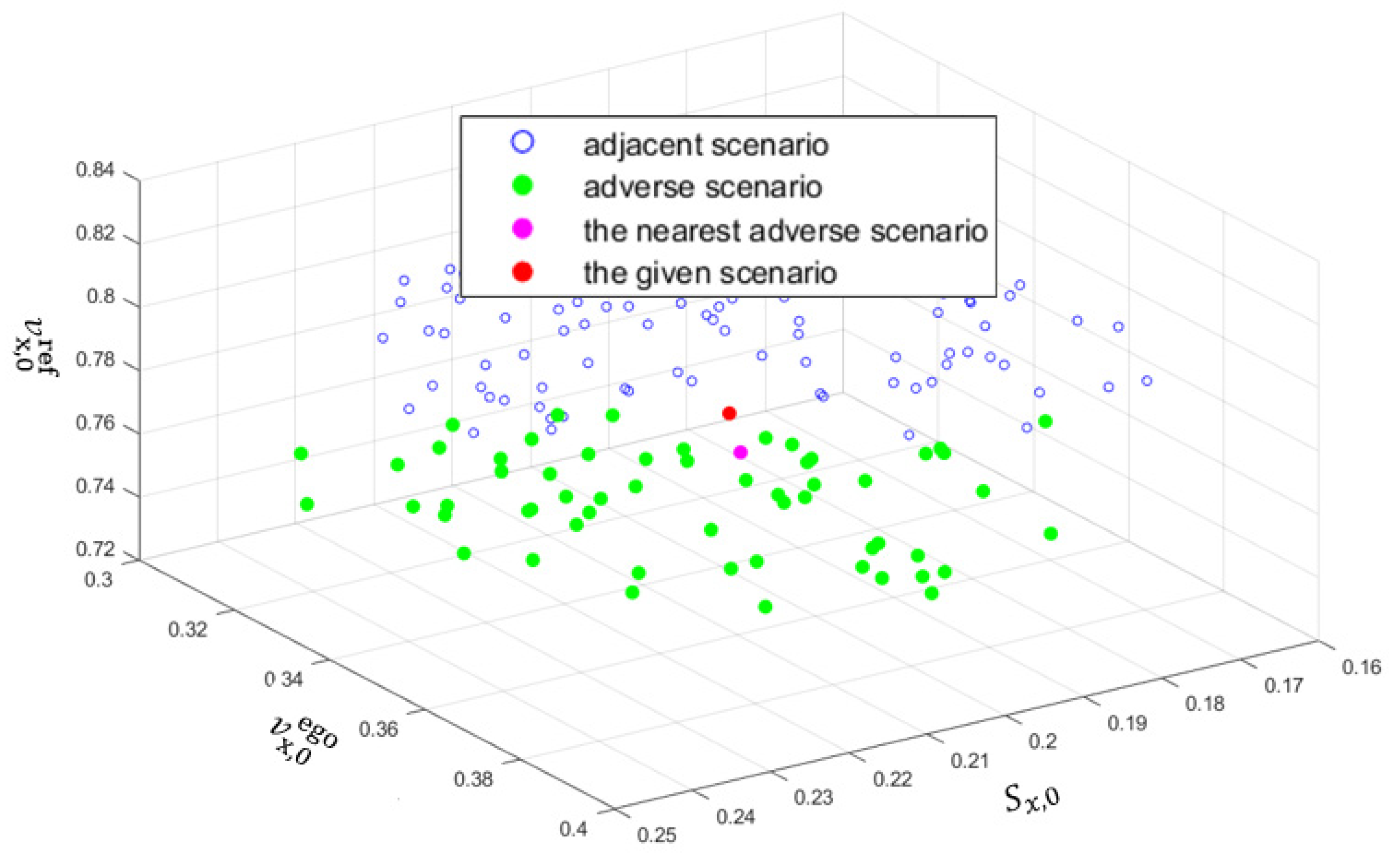
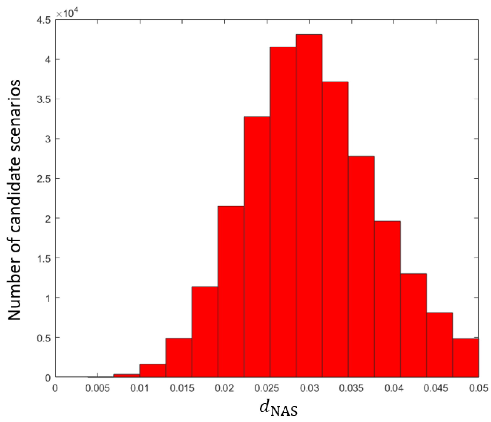
Before presenting the overall framework in the following section of the methodology, it is necessary to introduce some important terms and a distance-based approach for determining whether a scenario is near the performance boundary. First, several adjacent scenarios $\left\{S_{\mathrm{adj}}^i\right\}$ near the given scenario $S_0$ are generated by random sampling and executed one by one to determine their class labels based on the VUT performance. A scenario is critical if the VUT is responsible for a collision. Adverse scenarios $\left\{S_{\mathrm{adv}}^i\right\}$ are the adjacent scenarios that belong to the class different from the given scenario $S_0$.

For a given scenario $S_0$ from class 1, if at least one adverse scenario $S_{\mathrm{adv}}^i$ belonging to class 2 is found, the scenario $S_0$ is regarded as a boundary scenario, as shown in Figure 1. It is worth noting that the question of how close the given scenario needs to be to its adverse scenarios to be considered a boundary scenario is still an open question in this field. The threshold for distance may depend on various factors, such as the specific ODD, the performance requirements for the VUT, and the available resources to execute and evaluate scenarios. Therefore, more research is needed to determine a suitable threshold for different situations. In this study, the distance between the nearest adverse scenario $S_{\mathrm{adv}}^{\mathrm{nearest}}$ and the given scenario $S_0$ is expressed as $d_{\mathrm{NAS}}$. It is apparent that the smaller the $d_{\mathrm{NAS}}$ is, the closer the given scenario $S_0$ is to the performance boundary. It should be emphasized that the adverse scenarios of the given scenario are also boundary ones.

3.2. Overall Framework

This study aims to find diverse candidate scenarios consuming as few resources as possible. Three missions must be completed to achieve it. First, acquire an HPC that can accurately classify critical and non-critical scenarios in the ODD. Second, find a set of diverse candidate scenarios based on the HPC. Since high-dimensional candidate scenarios are rare in the ODD, the third mission is to obtain more diverse candidate scenarios based on a few.

The map between VUT performance and scenario parameters can be highly nonlinear and uncertain due to the complexity of HAV systems and natural traffic. Gaussian Process (GP) and Support Vector Machine (SVM) are widely used for classification and regression [51,52]. Compared with Artificial Neural Networks (ANN), SVM and GP can derive good results based on much less training data [53,54]. Furthermore, SVM is robust to outliers, and GP is good at capturing uncertainty and modeling nonlinear relationships. Therefore, SVM and GPC are both suitable for scenario classification. These two classifiers dig for information in the training data from different perspectives. SVM works on the structure information of the training data, while GPC minds information based on the probability theory. In this study, SVM and GPC guide each other in finding uncertain scenarios, improving the performance of both iteratively. If two classifiers generate two different class labels for one scenario, the scenario is considered uncertain. If two classifiers produce different class labels for a given scenario, that scenario can be considered to be an uncertain scenario. It is necessary to execute all uncertain scenarios to identify informative scenarios for both classifiers. By doing so, we can potentially obtain at least one HPC.

To identify candidate scenarios based on one HPC, several scenarios are generated by random sampling. Then, the HPC is used to classify all of these random scenarios. Finally, all candidate scenarios are identified using the distance-based method mentioned above.

Finally, the third mission is completed by local sampling, which can iteratively search for more candidate scenarios based on a small initial set of them.

3.3. Gaussian Processes

GP is a non-parametric machine-learning technique for pattern identification, regression, and classification [51]. For more details about GP, see [55,56]. “Non-parametric” does not mean that no parameters are needed, but because the relevant parameters are automatically optimized and do not need to be set by the user. A GP model is a set of random variables. The joint distributions of more than one of these random variables are joint Gaussian distributions [57]. A GP $f\left(x\right)$ can be represented by Equation (1):

$$f\left(x\right)~gp\left(m\left(x\right),k\left(x,x\prime \right)\right)$$

(1)

where $m\left(x\right)$ is a mean function often assumed to be 0 for convenience, $k\left(x,x\prime \right)$ is a covariance function.

A covariance function can be any function involving two inputs. Although many covariance functions exist, the most widely used one is the square exponential covariance function, as shown in Equation (2). According to the square exponential covariance function, if the distance between two samples increases, their correlation will decrease exponentially.

$$k\left(x,x^{\prime }\right)={\sigma }_f^2\exp \left(-\frac{1}{2l^2}{\left|x-x^{\prime }\right|}^2\right)$$

(2)

where ${\sigma }_f$ and $l$ are hyperparameters.

Given a training dataset $\mathcal{D}=\left\{x_i,y_i|i=1,\dots ,n\right\}$, where $n$ is the size of the training dataset, $x_i$ is a vector of inputs in $R^d$, $y_i$ is the observed outputs corresponding to $x_i$, as shown in Equation (3).

$$y_i=f\left(x_i\right)+ϵ$$

(3)

where $f\left(x_i\right)$ is the real output, $ϵ$ is an independent Gaussian noise with variance ${\sigma }^2$.

Based on the definition of GP, the distributions of the observed outputs $f$ and the predicted outputs $f_{*}$ can be described by Equation (4).

$$\left[\begin{array}{c}f\\ f_{*}\end{array}\right]~\mathcal{N}\left(0,\left[\begin{array}{cc}K+{\sigma }_n^{2}I& K_{*}^T\\ K_{*}& K_{**}\end{array}\right]\right)$$

(4)

where the mean function is assumed to be 0, $K=k\left(X,X\right)$, $K_{*}^T=k\left(X,X_{*}\right)$, $K_{*}=k\left(X_{*},X\right)$, $K_{**}=k\left(X_{*},X_{*}\right)$, $X\in {\mathcal{R}}^{d\times n}$ is a matrix of inputs in the training data ${\left\{x_i\right\}}_{i=1}^n$. $d$ is the dimension of the input space ${\mathcal{R}}^d$. $X_{*}$ is the matrix of test input.

Based on Bayesian theory, $f_{*}$ can be derived by Equation (5):

$$f_{*}|f,X,X_{*}~\mathcal{N}\left(K_{*}{K}^{-1}f,K_{**}-K_{*}{\left(K+{\sigma }_n^{2}I\right)}^{-1}{K}_{*}^T\right)$$

(5)

Therefore, given a test input $x_{*}$, the output of a GP model is the Gaussian distribution of $f_{*}\left(x_{*}\right)$, involving a mean and a variance, as shown in Equation (6). The mean is considered the predicted output for regression problems, and the variance indicates the confidence of the prediction.

$$\left\{\begin{array}{c}\mu \left(X_{*},\mathcal{D}\right)=K_{*}{K}^{-1}f\\ {\sigma }^2\left(X_{*},\mathcal{D}\right)=K_{**}-K_{*}{\left(K+{\sigma }_n^{2}I\right)}^{-1}{K}_{*}^T\end{array}\right.$$

(6)

For classification, the training data can be represented as $\mathcal{D}=\left\{x_i,y_i|i=1,\dots ,n,y_i=0,1\right\}$, where $y_i$ is the class label of $x_i$. The GP tackles classification problems by predicting the class probability $y_{*}$, which is the input of a logical function, deriving the predicted class. GPC mainly includes two steps. First, the distribution of the latent variable $f_{*}\left(x_{*}\right)$ is predicted. The class probability $y_{*}\left(x_{*}\right)$ is obtained as shown in Equation (7).

$$p\left(f_{*}|X,\mathrm{y},x_{*}\right)=\int p\left(f_{*}|X,x_{*},\mathrm{f}\right)p(\mathrm{f}|X,y)d\mathrm{f}$$

(7)

3.4. Support Vector Machines

SVM is a supervised learning technique proposed by Vapnik and has been used for pattern recognition, classification, and regression [52,58,59,60]. Unlike Artificial Neural Networks (ANN), SVM is built on solid theoretical foundations. For a detailed introduction to SVM, see [61,62]. In this study, SVM is used for classification. Rather than trying to find the classes for all training data as in other classification techniques, SVM aims to find maximum-margin hyperplanes that divide the feather space into several sub-spaces that belong to different classes. In other words, rather than aiming at minimizing empirical risk, SVM aims to minimize structural risk, making SVM robust to outliers and with a good generalization ability [63]. In a linear separable case, a training dataset is given as $\left\{x_i,y_i\right\}$ where $i=1,\dots ,l,x_i\in R^d,y_i\in \left\{-1,1\right\}$, $l$ is the size of the training dataset, $d$ is the dimension of $X_i$. 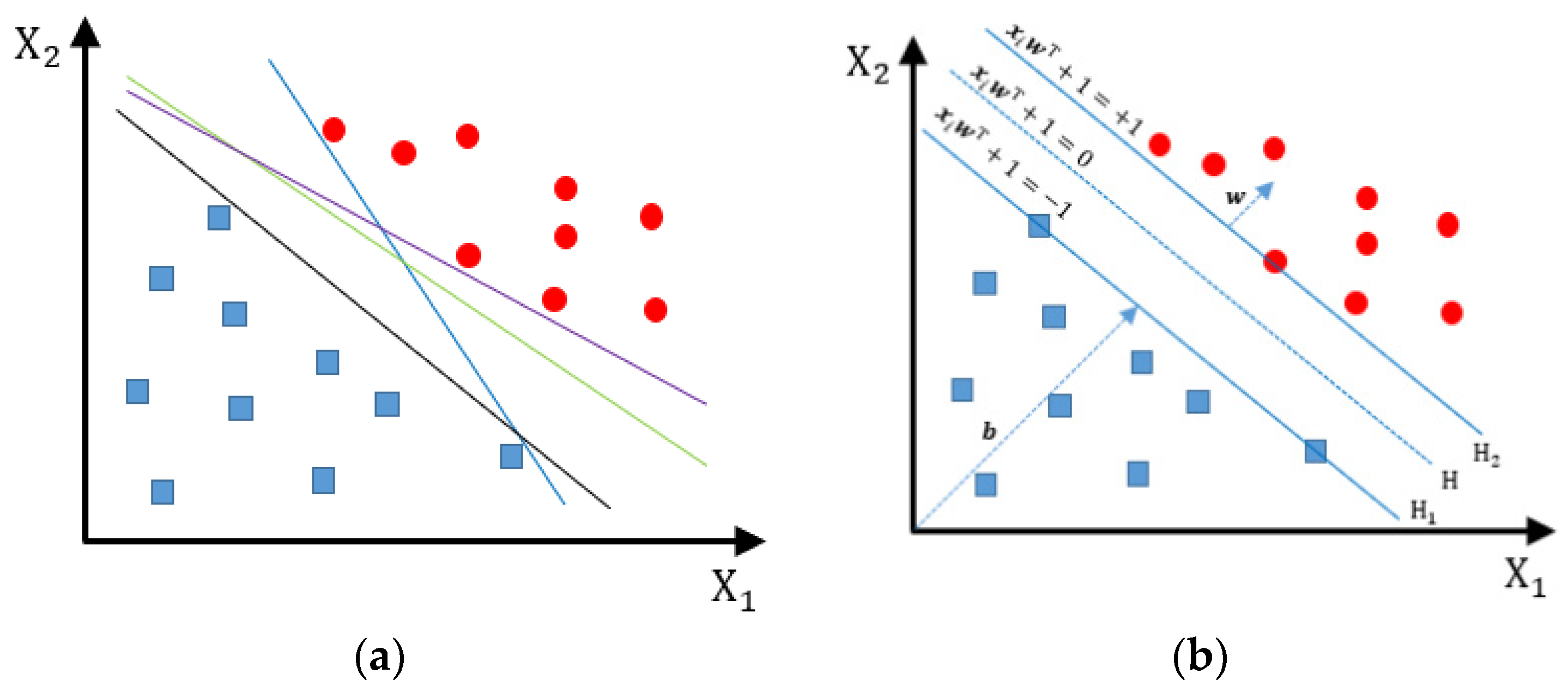$y_i$ can be 1 for one class or −1 for the other class. Therefore, the hyperplane that separates the training data can be described by $\left\{w,b\right\}$ in Equation (8) and Figure 2. The distance between the hyperplane and the nearest points is called the margin. It is obvious that there may be numerous hyperplanes. The purpose of SVM is to find the optimal hyperplane between two parallel hyperplanes, ${\mathrm{H}}_1$ and ${\mathrm{H}}_2$ [52]. There are no training data between ${\mathrm{H}}_1$ and ${\mathrm{H}}_2$. When the distance between ${\mathrm{H}}_1$ and ${\mathrm{H}}_2$ is maximized, the training points on them are called support vectors.

$$\left\{\begin{array}{c}\left\{w,b\right\}:x_i{w}^{\mathrm{T}}+1=0, \forall i\\ y\left(x_i{w}^{\mathrm{T}}+b\right)\ge 1, c=+1\\ y\left(x_i{w}^{\mathrm{T}}+b\right)\le -1, c=-1\end{array}\right.$$

(8)

where $w$ is normal to the hyperplane $\left\{w,b\right\}$, $||w||$ is the Euclidean norm of $w$, $w$ and $b$ are scalable.

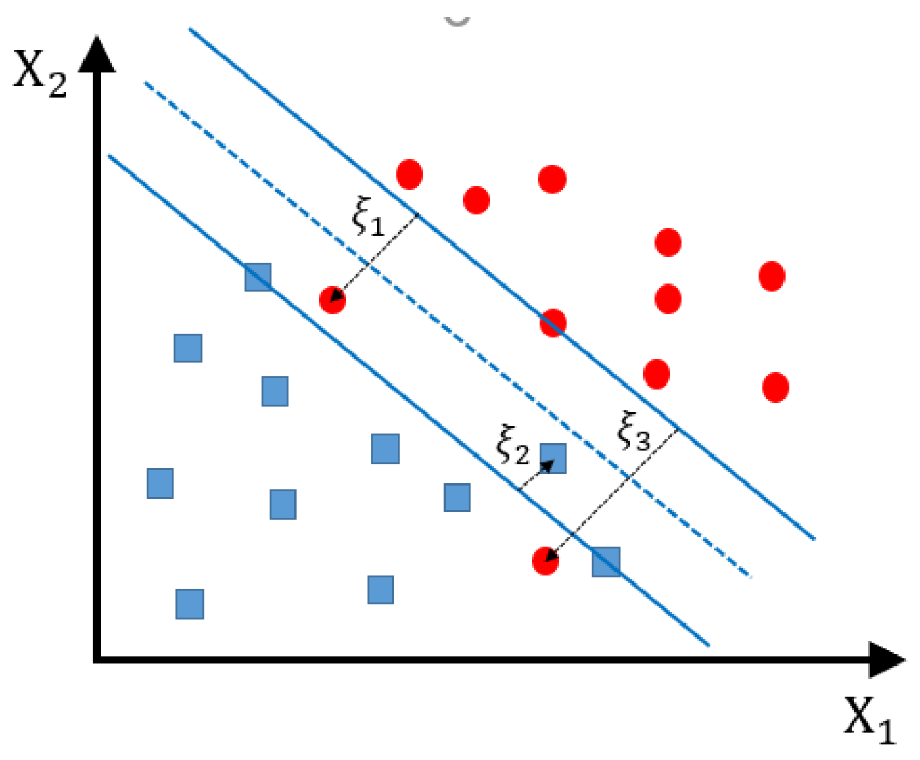
If the training is not linearly separable, no hyperplanes can separate the training data, which usually happens in practical cases. There are two solutions to tackle this problem. First, slack variables ${\xi }_i$ are introduced, as shown in Figure 3. Then, the problem of finding the optimal hyperplane is equivalent to the minimization of $\frac{||w||}{2}+C{\displaystyle \sum }_i^l{\xi }_i{}^2$, where $C$ is the penalty parameter that controls the width of the soft margin, as shown in Equation (9). The Lagrangian for maximizing the soft margin is shown in Equation (10).

$$\left\{\begin{array}{c}\left\{w,b\right\}:y\left(x_i{w}^{\mathrm{T}}+b\right)+{\xi }_i=1,{\xi }_i\ge 0\\ y\left(x_i{w}^{\mathrm{T}}+b\right)\ge 1-{\xi }_i, c=+1, {\xi }_i\ge 0\\ y\left(x_i{w}^{\mathrm{T}}+b\right)\le -1+{\xi }_i, c=-1,{\xi }_i\ge 0\end{array}\right.$$

(9)

$$L\left(w,b,\xi ,\alpha \right)=\frac{1}{2}{||w||}^2-{\displaystyle \sum }_{i=1}^l{\alpha }_i\left[y_i\left(x_i·w^{\mathrm{T}}+b-1+{\xi }_i\right)\right]+\frac{C}{2}{\displaystyle \sum }_{i=1}^l{\alpha }_i$$

(10)

If a linear SVM cannot yield good results even though the margin between two classes has been maximized, a nonlinear SVM is needed to tackle the problem. The nonlinear SVM works based on the assumption that the training data that are not linearly separable in the original space $R^d$ tend to be linear separable after being mapped by a function $\varphi$ to a high-dimensional feather space $R^f$. Therefore, the most significant difference between linear SVM and nonlinear SVM is that the hyperplanes exist in the feather space $R^f$ rather than the original space $R^d$. It is not easy to find the best mapping function $\varphi$. However, based on the Lagrangian shown by Equation (10), the kernel function $K$ (Equation (11)) can achieve our purpose indirectly.

$$K\left(x_i,x_j\right)=\varphi \left(x_i\right)\varphi \left(x_j\right)$$

(11)

There are many popular kernel functions, as shown in

Table 1. Some popular kernel functions.

Name	Equation
Linear Kernel	$k\left(x,y\right)=x^{\mathrm{T}}y+c$
Polynomial Kernel	$k\left(x,y\right)=a{x}^{\mathrm{T}}y+c^d$
Radial Basis Function	$k\left(x,y\right)=\exp (-\gamma {||x-y||}^2)$
Gaussian Kernel	$k\left(x,y\right)=\exp (-\frac{{||x-y||}^2}{2{\sigma }^2})$
Exponential Kernel	$k\left(x,y\right)=\exp (-\frac{||x-y||}{2\sigma })$

. This study uses the Gaussian kernel function for classification based on SVM.

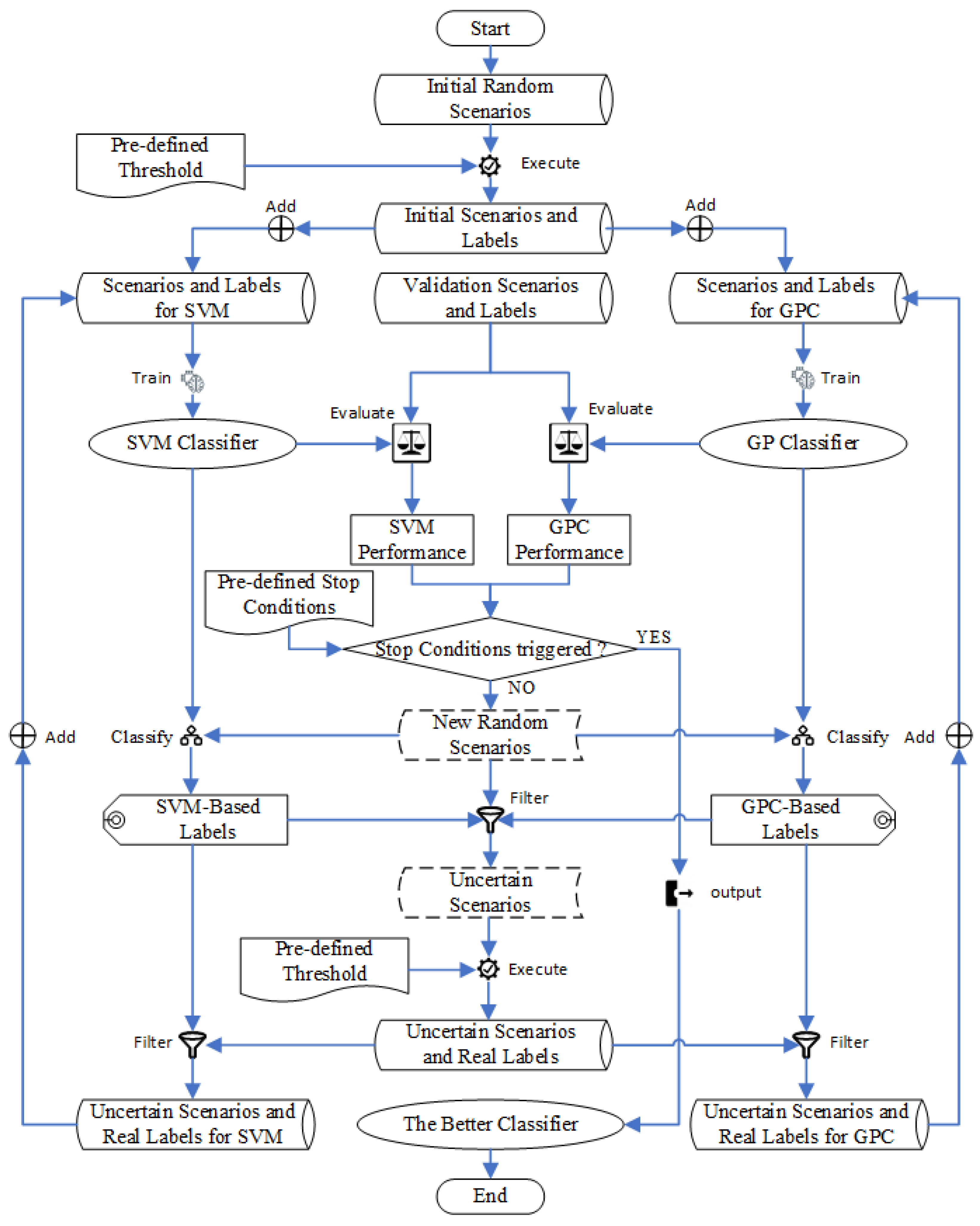
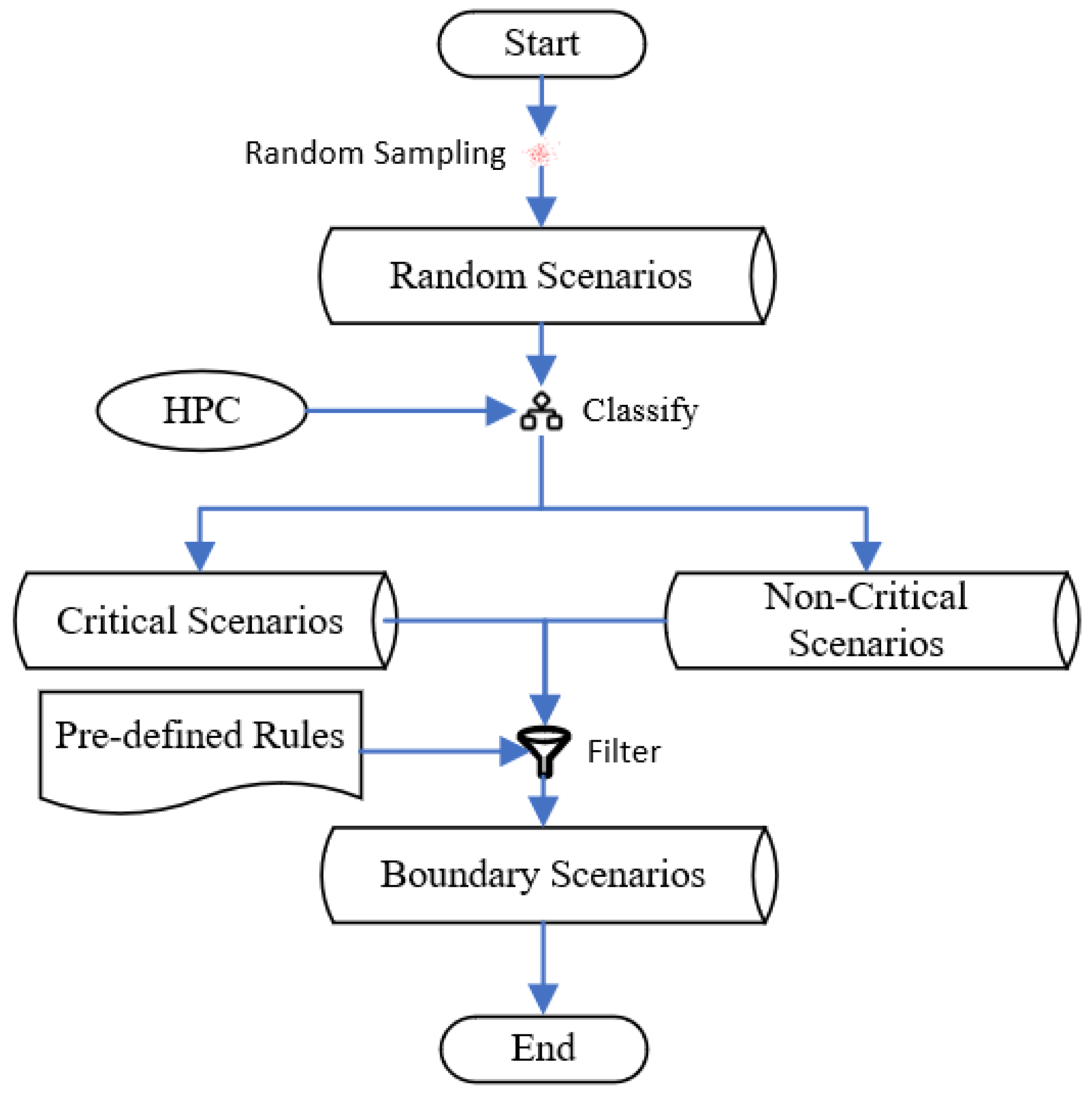
3.5. Obtaining High-Performance Classifiers

This study proposes a strategy for obtaining an HPC, as illustrated in Figure 4. In this strategy, SVM and GPC classifiers guide each other to iteratively identify uncertain scenarios that improve their respective performances. A scenario is considered uncertain if it is classified differently by the SVM and GPC classifiers. This strategy can be divided into five steps:

Step 1: the initial scenarios are randomly generated and executed. Their class labels are generated based on a pre-defined criticality metric and a threshold. For example, “1” is the label for critical scenarios, and “0” is for non-critical scenarios. The initial scenario dataset with labels will be used as a training dataset for SVM and GPC in Step 2.

Step 2: The SVM and GPC classifiers are trained based on their respective training datasets.

Step 3: A test dataset is used to evaluate the performance of the SVM and GPC classifiers. If pre-defined conditions are met, the iteration stops. If not, the next step is executed.

Step 4: Generate random scenarios again. The classifiers obtained in Step 2 are used to label them. Therefore, all uncertain scenarios can be identified.

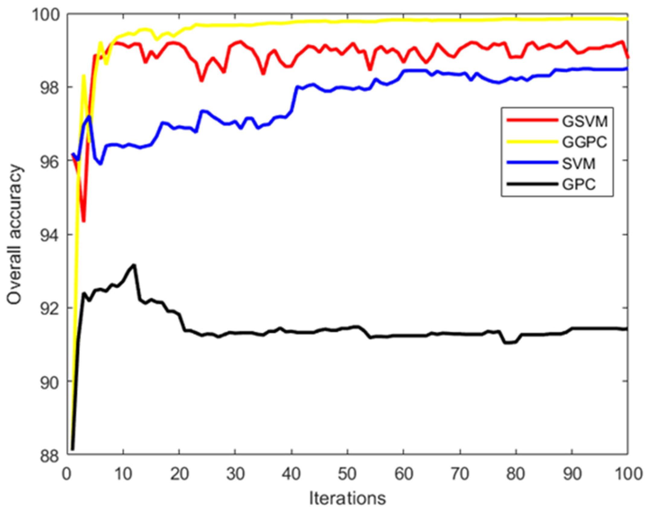
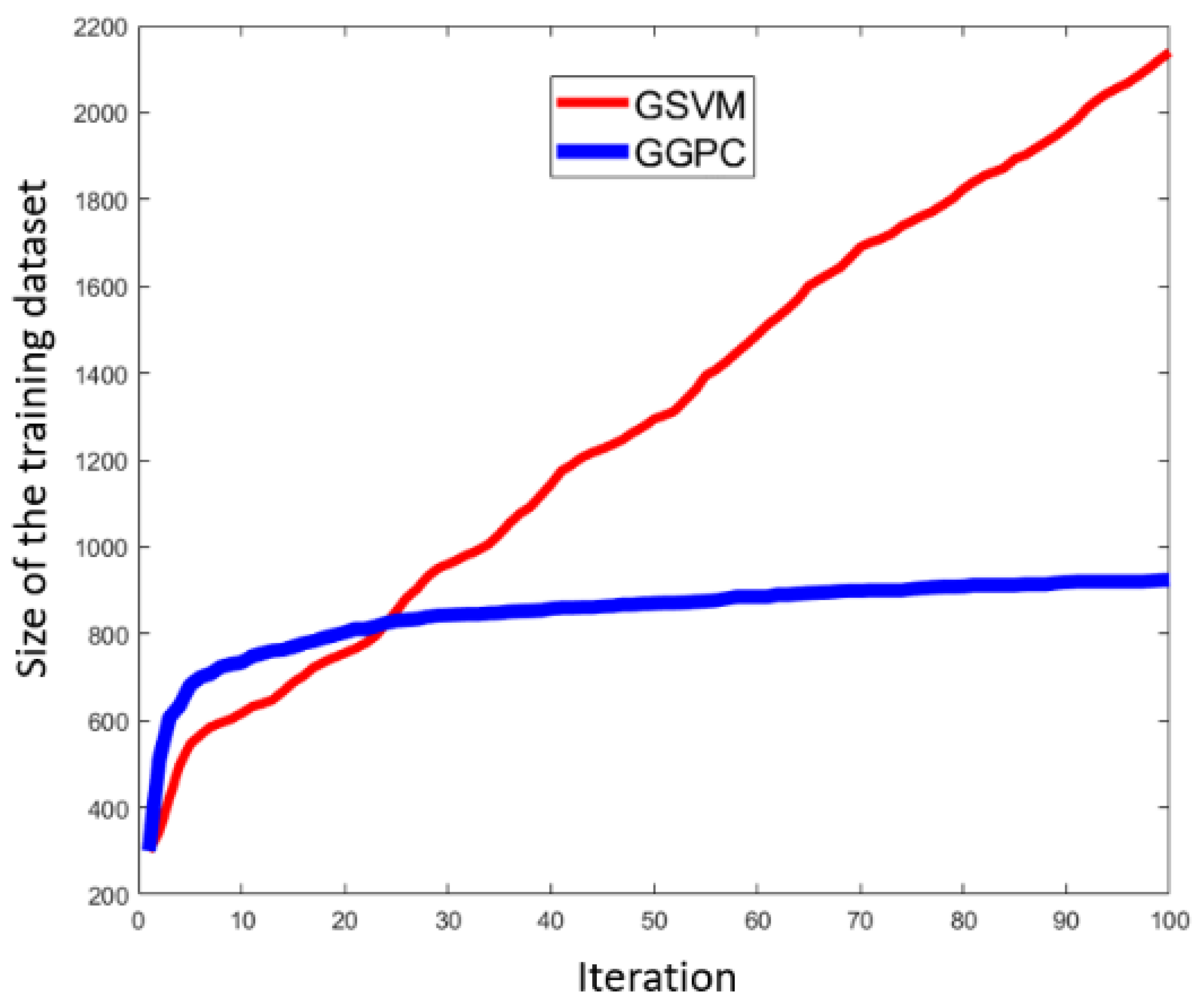
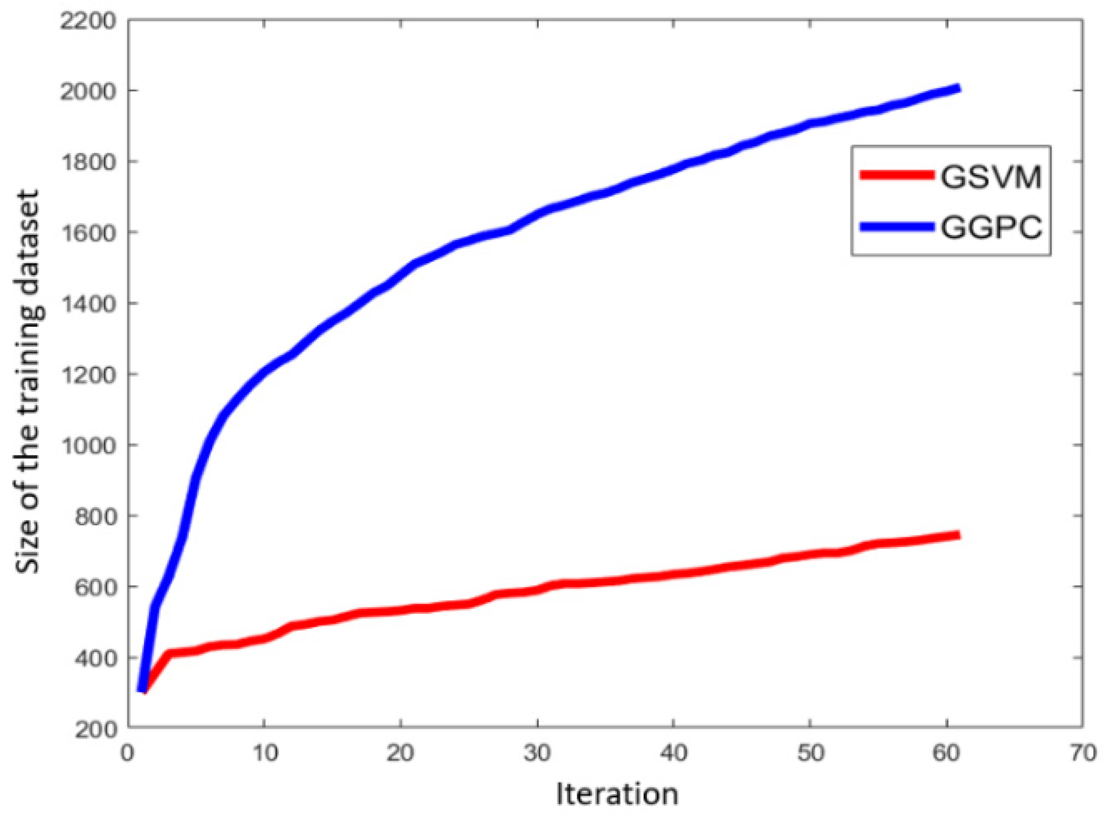
Step 5: All uncertain scenarios identified in Step 4 are executed, and their real labels are acquired based on the pre-defined criticality threshold. The uncertain scenarios that the SVM or GPC did not classify correctly are added to the training dataset for SVM or GPC, updating the training dataset. The iteration goes back to Step 2 until at least one of the stop conditions is met. Finally, the better of the two classifiers is selected as the HPC for scenario classification. For convenience, the SVM and GPC classifiers obtained using this method are called the Guided SVM (GSVM) model and the Guided GPC (GGPC) model, respectively.

3.6. Searching for Candidate Scenarios Based on an HPC

To identify candidate scenarios based on one HPC, the method shown in Figure 5 can be used, which involves two iterative steps.

Step 1: Several scenarios are generated by random sampling, and their labels are derived based on the HPC.

Step 2: All candidate scenarios in the random scenario dataset are identified based on the distance-based method described in Section 3.1. It is worth noting that the labels of the random scenarios are all derived based on the HPC rather than scenario execution.

Using this method, candidate scenarios can be efficiently identified, and further scenario execution can be focused on informative scenarios that can improve the classifier performance. This approach can help reduce the consumption of computing resources and make the process more efficient.

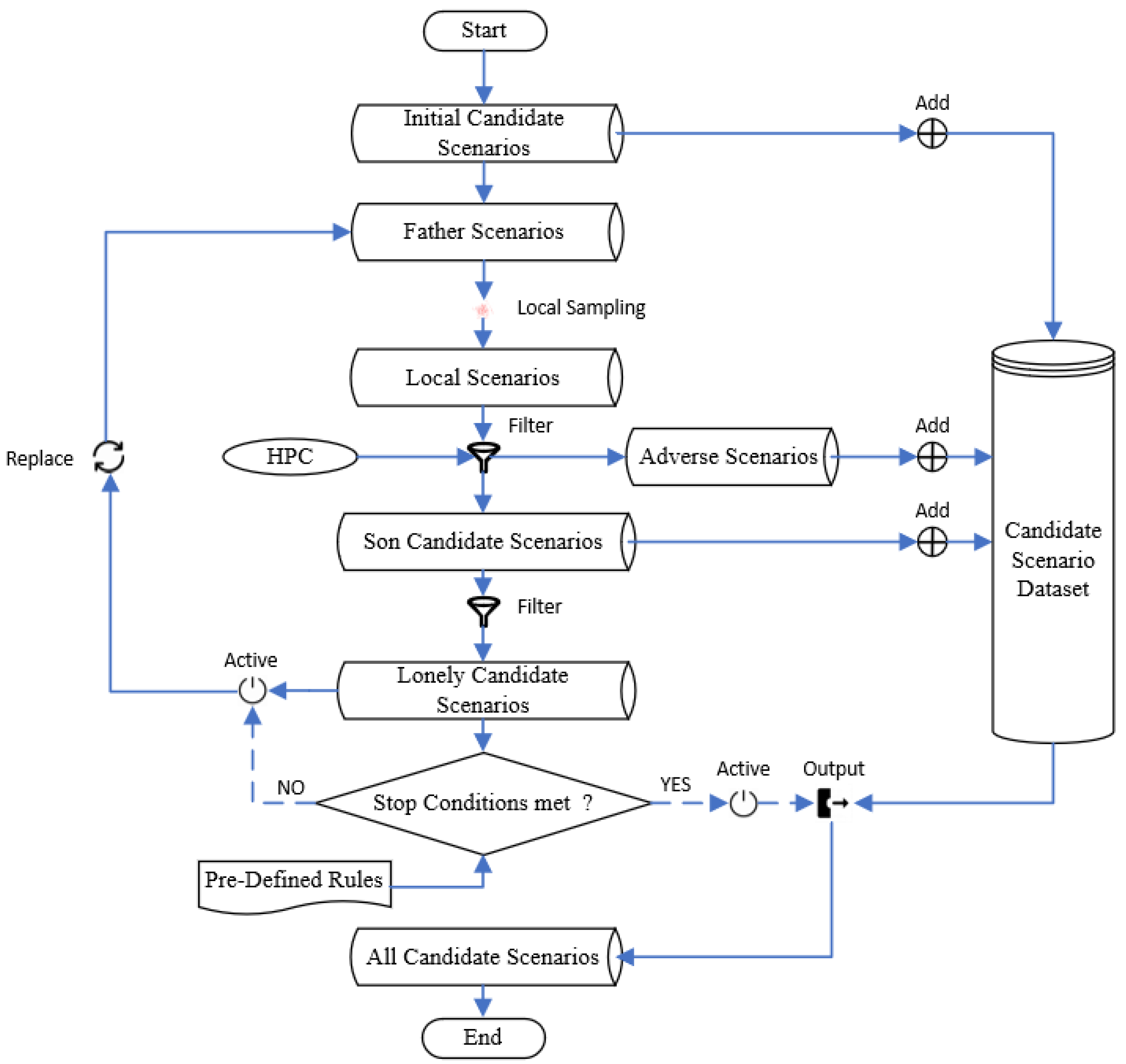
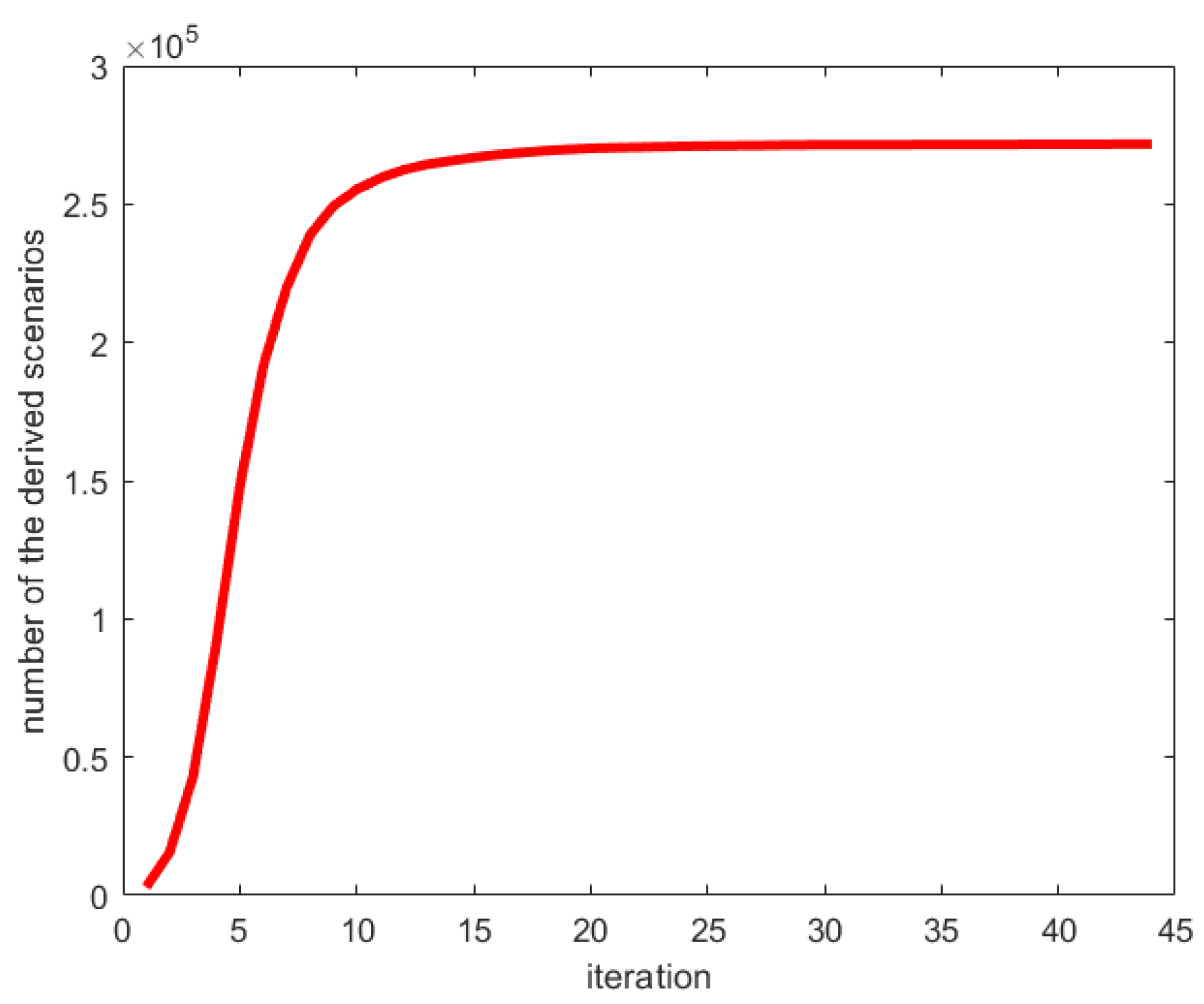
3.7. Generating Diverse Candidate Scenarios by Local Sampling

Theoretically, it is possible to generate numerous candidate scenarios based on one HPC by classifying many random scenarios. However, high-dimensional boundary scenarios in a random scenario set are rare, which means that a significant number of random scenarios would be required to identify the candidate ones based on the HPC. This process can consume many computing resources, even though no scenario execution is involved.

This study proposes a method to efficiently identify diverse candidate scenarios by deriving many boundary scenarios based on a small set of them. The method consists of five steps, as shown in Figure 6.

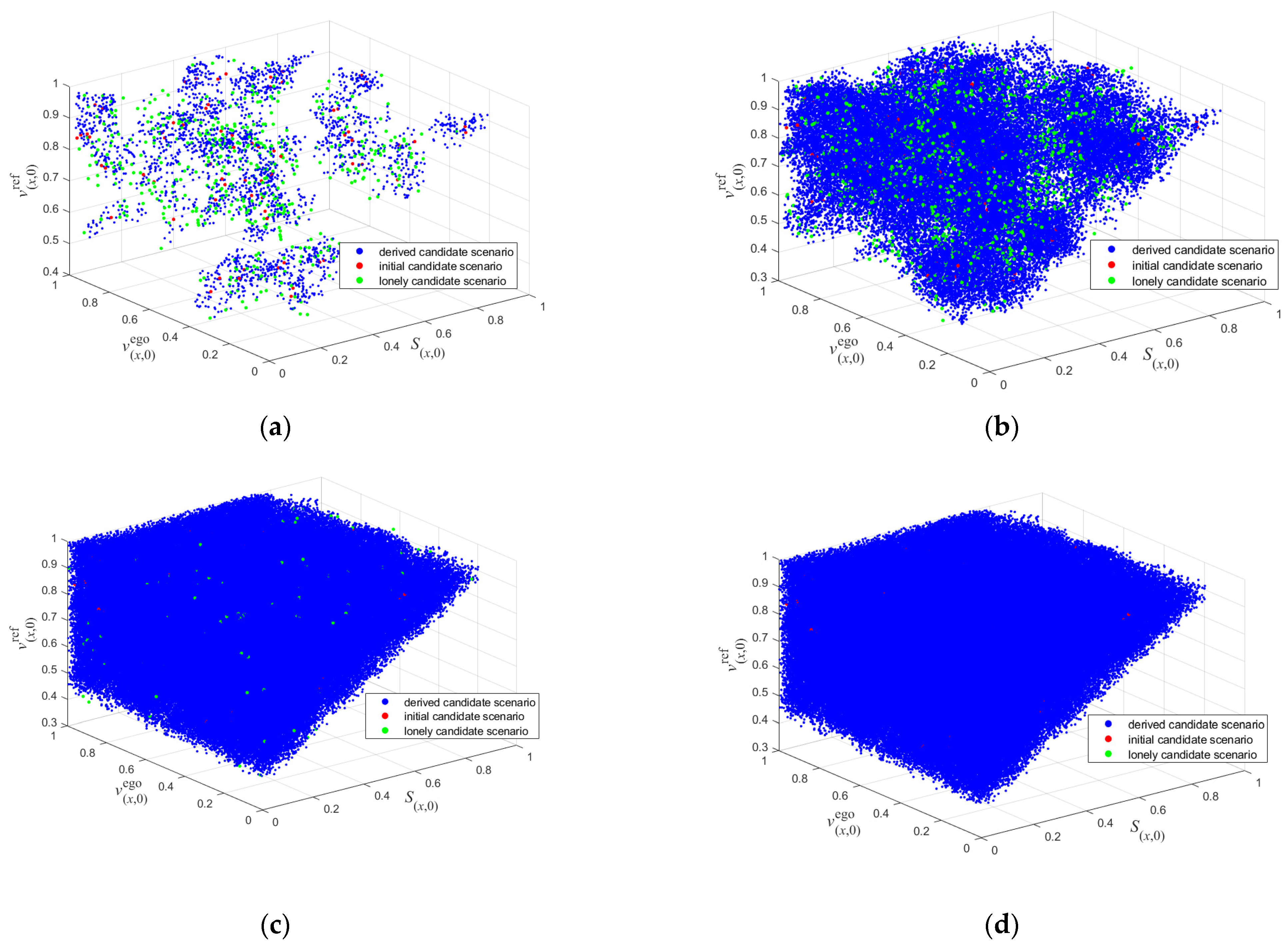
Step 1: Local sampling. Generate adjacent scenarios $\left\{S_{\mathrm{adj}}^i\right\}$ around each father candidate scenario $S_{\mathrm{fat}}^j$. For convenience, the candidate scenarios in the given candidate scenario dataset are called father candidate scenarios, and the candidate scenarios generated by local sampling are called son candidate scenarios.

Step 2: Find son candidate scenarios. Identify son candidate scenarios in the scenarios generated in Step 1 based on the distance-based method described in Section 3.1.

Step 3: Identify lonely candidate scenarios. The lonely candidate scenarios do not have enough adjacent scenarios around. All lonely candidate scenarios can be identified by checking the distance between scenarios. Then, the lonely scenarios are considered father scenarios. Iterate Steps 1 to 3 until pre-defined conditions are met, which can be iterating enough times, or the number of lonely candidate scenarios is less than a threshold et al.

4. Simulation Experiments

4.1. Testing Scenarios

Car-following and cut-in scenarios are common in highway and urban traffic. Therefore, it is significant to test the car-following and cut-in functions of HAVs. Therefore, it is essential to evaluate the performance of HAVs in these scenarios. For simplicity, in this study, car-following and cut-in scenarios involving an ego vehicle and a reference vehicle are considered, as shown in Figure 7.

In the car-following scenario, the following vehicle is the ego vehicle, and the leading vehicle is a reference vehicle moving at a constant longitudinal speed $v_{\mathrm{x},0}^{\mathrm{front}}$. All vehicles in the car-following scenario remain in their lanes. As shown in Figure 7a, the car-following scenario involves three parameters: the initial distance between the ego and reference vehicles $S_{x,0}$, the initial velocity of the reference vehicle $v_{\mathrm{x},0}^{\mathrm{front}}$, and the initial velocity of the ego vehicle $v_{\mathrm{x},0}^{\mathrm{ego}}$. The parameter ranges for the car-following scenario are presented in

Table 2. Parameter settings for the simplified car-following scenario.

Description	Key Parameter	Value Range
the initial distance between the two vehicles	$S_{x,0}$	(15, 100) m
the initial velocity of the ego vehicle	$v_{\mathrm{x},0}^{\mathrm{ego}}$	(5, 40) m/s
the initial velocity of the reference vehicle	$v_{\mathrm{x},0}^{\mathrm{ref}}$	(5, 40) m/s

. The car-following scenario ends immediately if a crash occurs.

In the cut-in scenario, the lane-change vehicle is a reference vehicle, and the other vehicle is the ego vehicle. For simplicity, the longitudinal and lateral speeds of the reference vehicle are assumed to be constant during lane changing. As shown in Figure 7b, four parameters can be used to describe the cut-in scenario, the initial longitudinal distance between two vehicles $S_{x,0}$, the initial lateral distance of the reference vehicle $S_{y,0}$, the initial longitudinal speed of the ego vehicle $v_{x,0}^{\mathrm{HAV}}$, the initial longitudinal speed of the reference vehicle $v_{x,0}^{\mathrm{front}}$, the initial lateral speed of the reference vehicle $v_{y,0}^{\mathrm{front}}$. The parameter ranges for the cut-in scenario are presented in

Table 3. Parameter settings for the simplified cut-in scenario.

Description	Key Parameter	Value Range
the initial longitudinal distance between two vehicles	$S_{x,0}$	(15, 100 m
initial lateral distance between two vehicles	$S_{y,0}$	(1.9, 3.8) m
initial longitudinal speed of the ego vehicle	$v_{x,0}^{\mathrm{ego}}$	(10, 40) m/s
initial lateral speed of the reference vehicle	$v_{y,0}^{\mathrm{ref}}$	(0.5, 1.75) m/s
initial longitudinal speed of the reference vehicle	$v_{x,0}^{\mathrm{ref}}$	(10, 35) m/s

, while

Table 4. Other parameters for the car-following scenario and the cut-in scenario.

Description	Key Parameter	Value
vehicle width	$w_{veh}$	1.8 m
vehicle length	$l_{veh}$	5 m
lane width	$w_{lane}$	3.8 m
the maximum duration of the scenario	$T_{\max }$	10 m

describes other critical parameters for the car-following and cut-in scenarios. The ego vehicle starts to cut in at the beginning of the cut-in scenario, and if no collision occurs, the scenario will end three seconds after the lane-change process is completed. In the case of a collision, the scenario ends immediately. If no collision occurs, the reference vehicle continues to drive at a constant longitudinal speed after the lane change. The simulation duration for the car-following and cut-in scenarios is limited to 10 s, with a simulation step size of 0.01 s.

4.2. Intelligent Driver Model

The Intelligent Driving Model (IDM) is a widely used microscopic traffic simulation model that controls a vehicle’s longitudinal movement to prevent front-end collisions. However, when the distance between the leading and following vehicles is extremely small, the IDM may produce an excessive and unreasonable acceleration to avoid a collision. To prevent this, the maximum deceleration is limited to $b_{\max }=5 \mathrm{m}/{\mathrm{s}}^2$, which keeps vehicle decelerations within a reasonable range [64]. This study adopts the modified IDM model with this setting as the VUT. The parameter values for the modified IDM model used in this study are presented in

Table 5. Parameter settings for the IDM model.

Description	Key Parameter	Typical Value
Desired velocity	$v_d$	29.8 m/s
Safe time headway	$T$	1.6 s
Maximum acceleration	$a$	2.62 m/s2
Desired deceleration	$b$	2.67 m/s2
Acceleration exponent	$\delta$	4
Jam distance 1	$s_0$	1 m
Jam distance 2	$s_1$	2 m
Vehicle length	$l$	5 m

.

4.3. Stop Conditions

When training classifiers, the size of the initial random scenarios is 300. In each iteration, 2000 scenarios are randomly generated to search for uncertain scenarios. In simulation experiments, the stop conditions include: The size of training data for one or both classifiers is over 3000; In the latest 15 iterations, the fluctuation of the classification accuracy of at least one classifier is less than 0.01%; At least one of the classifiers achieves a classification accuracy of 100%.

When deriving candidate scenarios based on local sampling, the iteration stops if no more lonely scenarios can be found.

4.4. Distance Thresholds for Determining Candidate or Boundary Scenarios

Furthermore, the distance thresholds for determining candidate or boundary scenarios based on the distance-base method described in Section 3.1 are 0.02 and 0.05 for car-following and cut-in scenarios, respectively. It needs to be noticed that all these thresholds are normalized Euclidean distances.

4.5. Criticality Metric

In the car-following and cut-in scenarios, Equation (12) is used to calculate the criticality of the scene at time $t$. The smallest criticality during the scenario is adopted to measure the criticality of the scenario. If the longitudinal speed of the ego vehicle is higher than that of the reference vehicle, TTC is used as the criticality metric. If not, a penalty of 100 is assigned. For the cut-in scenario, if the reference vehicle collides with the ego from the right, the reference vehicle should be responsible because the behavior of the ego vehicle is stable and predictable, and the lane-change vehicle should stop cutting in before crashing according to the traffic law.

$$C_s\left(t\right)=\left\{\begin{array}{c}\frac{x_{lead}\left(t\right)-x_{follow}\left(t\right)}{v_{follow}\left(t\right)-v_{lead}\left(t\right)}, if v_{follow}>v_{lead}\\ 100, if v_{follow}\le v_{lead}\end{array}\right.$$

(12)

All training and testing data are normalized to mitigate the negative effects of the ranges of different parameters. To quantify the effectiveness and efficiency of the methodology proposed in this study, Two SVM and GPC classifiers are trained by random scenarios. The numbers of training data for SVM and GSVM are the same. In addition, so are those for GPC and GGPC. To increase the number of critical scenarios in the test dataset, some critical scenarios are generated by PSO [29].

5. Numerical Results and Discussions

5.1. Results and Discussions of Car-Following Scenario Experiments

In the experiments involving car-following scenarios, there are 10,078 scenarios in the test dataset, including 808 and 78 critical scenarios obtained by random sampling and PSO, respectively. The performance curves of GSVM, GGPC, SVM, and GPC are presented in Figure 8. With new samples added to the training datasets, all performance curves fluctuate. After ten iterations, the accuracy of GGPC increases from 88.12% to 99.39%, outperforming all other classifiers. GSVM performs better than GPC and SVM, achieving an accuracy of 99.16%. After 23 iterations, no significant improvements happened to GGPC. The performance of GSVM fluctuates between 98% and 99% after ten iterations. New training data for GPC cannot make it perform much better after the 12th iteration. The overall trend of the performance curve of SVM indicates that the accuracy of SVM might become better after the 100th iteration. However, the iteration is stopped because of the stagnation of the accuracy of GGPC in the latest 15 iterations. It is worth noting that the fluctuation of GGPC is much less significant than that of GSVM, which indicates that the former is better at capturing uncertainties in this case. Test samples labeled by GGPC are presented in Figure 9, indicating that the samples that GGPC cannot classify correctly are near the performance boundary.

Table 6. Performance of the classifiers on the car-following scenario.

Metrics	GPC	SVM	GGPC	GSVM
True Positive Rate (TPR)	66.02%	82.90%	99.66%	98.75%
True Negative Rate (TNR)	93.86%	100%	99.87%	98.77%
False Positive Rate (FPR)	6.14%	0	0.13%	1.23%
False Negative Rate (FNR)	33.98%	17.10%	0.34%	1.25%
Overall Accuracy	91.42%	98.50%	99.85%	98.77%

details the performance of all four classifiers at the end of simulation experiments. Positive indicates critical, and vice versa. GPC is the worst one among all four classifiers. Compared with GPC, GGPC performs much better with TPR, TNR, FPR, and FNR improved by 55.95%, 6.20%, 97.88%, and 99.00%, respectively, showing that the guidance of GSVM can significantly enhance GGPC. SVM can successfully identify all non-critical scenarios in the test dataset, while 17.10% of critical scenarios are labeled non-critical ones. The TPR of SVM is 82.90% worse than that of GGPC and GSVM. The overall accuracy of GSVM is 98.77%, a little better than that of SVM, 98.50%, as shown in Table 6. It is worth noting that only 1.25% of critical scenarios are falsely identified as non-critical scenarios, indicating that under the guidance of GGPC, GSVM can identify critical scenarios much better than SVM.

Figure 10 provides the sizes of the training datasets for GGPC and GSVM in each iteration. As the experiment progresses, the number of new uncertain scenarios discovered by GGPC decreases more quickly than that of GSVM after the 24th iteration, indicating that GGPC performs better than GSVM in generating high-quality boundary scenarios. In the end, GSVM is trained using 2139 data, while GGPC uses 923 data. However, the difference in the overall accuracy between GSVM and GGPC in classifying the test dataset (Table 6) is insignificant, possibly due to the lack of diverse critical scenarios in the test dataset.

We aim to generate candidate scenarios effectively and efficiently. To evaluate the performance of our classifiers in achieving this goal, we randomly sample a scenario dataset of one million scenarios. We then use four classifiers to detect boundary scenarios in this dataset based on the distance-based method described in Section 3.1. The simulation results are presented in Table 6, and the training dataset sizes for GSVM and GGPR are plotted in Figure 10. GGPC identifies 2329 candidate scenarios, of which 2301 are boundary scenarios—significantly better than all other classifiers. It is worth noting that the mean distance between boundary scenarios found by GGPC and their corresponding NSOCs is 0.015, as shown in

Table 7. Performance of the four classifiers in generating high-quality candidate scenario sets.

Method	Number of Candidate Scenarios	Number of Boundary Scenarios	The Proportion of Boundary Scenarios	Mean Distance to the NAS
GPC	7866	1346	17.11%	0.017
SVM	2120	1308	61.70%	0.017
GGPC	2329	2301	98.80%	0.015
GSVM	2348	1562	66.52%	0.017

, which is also better than all other classifiers. Among all candidate scenarios identified by GPC, only 17.11% were boundary ones. GSVM find 1562 boundary scenarios, achieving a rate of 66.52%—better than the performance of SVM. In conclusion, the GGPC obtained through the methodology proposed in this study performs well in detecting boundary car-following scenarios.

The number of candidate scenarios found by GGPC is 2329, and 98.80% are boundary ones. It is enough to obtain the performance boundary of the car-following scenario in the ODD by Locally weighted smoothing linear regression, as shown in Figure 11. In Figure 12, most critical scenarios are above the performance boundary except some near it, and almost all non-critical scenarios are below it, which means that the deriving boundary surface can divide the critical and non-critical sub-spaces in the ODD effectively. To prove it quantitatively, ten thousand points on the $S_{x,0}-v_{\mathrm{x},0}^{\mathrm{ego}}$ surface are generated randomly. Then, they are projected to the performance boundary, obtaining 3854 candidate scenarios. A total of 99.87% of them are boundary scenarios based on scenario executions. The mean distance between these candidate scenarios and their NASes is 0.0057, much smaller than the threshold of 0.02.

5.2. Results and Discussions of Cut-In Scenario Experiments

In the cut-in scenarios experiments, the test dataset has 10,118 scenarios, with 620 and 245 critical scenarios obtained by random sampling and PSO-based searching. The performance of the four classifiers in cut-in scenario experiments is shown in Figure 13. GPC is the worst, with overall classification accuracy consistently below 87%. SVM performance is much better than GPC, whose accuracy is above 96%. After three iterations, it achieves its best accuracy, 97.37%, and then fluctuates between 96.5 and 97.5%. Similar to SVM, the accuracy of GSVM increases from 95.25% to 99.47% and then fluctuates between 98.60% and 99.60%. The performance of GGPC is not better than that of SVM in the first eight iterations. However, the accuracy of GGPC rapidly increases and reaches 98.27% in the tenth iteration under the guidance of GSVM. Then, the performance of GGPC gradually improves and obtains an accuracy of 99.33% in the last iteration, which is a bit better than that of GSVM.

Table 8. Performance of the classifiers on the cut-in scenario.

	GPC	SVM	GGPC	GSVM
True Positive Rate	60.65%	49.52%	97.10%	97.90%
True Negative Rate	88.11%	100%	99.47%	99.45%
False Positive Rate	11.89%	0	0.53%	0.55%
False Negative Rate	39.35%	50.48%	2.90%	2.10%
Overall Right Rate	86.43%	96.91%	99.33%	99.36%

presents the performance of all classifiers at the end of the last iteration. The overall accuracy of SVM is better than GPC. However, the TPR and FNR are around 50%, which is intolerable for binary classification. GGPC and GSVM perform much better than GPC and SVM, which can accurately classify 99.33% and 99.36% of all scenarios in the test dataset, respectively, and more importantly, their TPR and TNR are all above 97%.

The curves of training data sizes of GGPC and GSVM are provided in Figure 14. In each iteration, new uncertain scenarios are found for both GGPC and GSVM, but the size of the training data for GGPR is always smaller than that for GSVM due to fewer uncertain scenarios detected by GGPC. At the end of the experiment, GSVM is trained based on 745 data while GGPC is trained on 2007 data. In the last iteration, 18 uncertain scenarios are found, and GSVM correctly classifies 11 while GGPC only successfully labels seven of them. Therefore, it may be concluded that GSVM performs better than GGPC, even though the overall accuracy of GGPC is slightly better than that of GSVM in classifying the test dataset, as shown in Table 8.

To evaluate the performance of the classifiers in generating boundary cut-in scenarios, a dataset of 20,000 random scenarios is generated. Then, four classifiers are used to detect candidate scenarios in the dataset. The simulation results are presented in

Table 9. Performance of the four classifiers in generating boundary cut-in scenarios.

Method	Candidate Scenarios	Boundary Scenarios	Proportion of Boundary Scenarios	Mean Distance to the NAS
GPC	489	50	10.22%	0.033
SVM	52	17	32.69%	0.037
GGPC	111	88	79.28%	0.031
GSVM	106	97	91.51%	0.031

. GPC identifies 489 candidate scenarios, but only 9.61% of them are boundary scenarios. SVM finds 52 candidate scenarios, and 32.69% of them are boundary scenarios, which is better than GPC. GGPC identifies 111 candidate scenarios, out of which 88 are boundary scenarios, indicating that GGPC outperforms GPC and SVM. Finally, GSVM is found to be the best classifier, which identifies 106 candidate scenarios, out of which 91.51% are boundary scenarios.

Since five parameters are used to describe the cut-in scenario, boundary cut-in scenarios are much rarer than boundary car-following scenarios. It is necessary to generate more candidate scenarios based on local sampling, as described in Section 3.7. Parameter settings for boundary scenario deriving are presented in Table 9

Based on the 106 candidate scenarios found by GSVM above, 271,744 candidate scenarios are generated by iterative local sampling, and 86.10% are boundary scenarios. The number of the derived candidate scenarios after each iteration is shown in Figure 15. Derived, initial, and lonely candidate scenarios at the end of each iteration are visualized in Figure 16. Although the cut-in scenario involves five parameters, only three are included in Figure 16. All derived candidate scenarios can be used to test HAVs.

Figure 17 shows the distribution of distances between candidate scenarios and their nearest adverse scenarios. Given a boundary scenario, generating random scenarios around it can help identify adverse scenarios. However, the further the boundary scenario is from the performance boundary, the more difficult it is to find an adverse scenario. This explains the decreasing trend in the graph in Figure 17 after a distance of approximately 0.03. For a boundary scenario that is too close to the performance boundary, it is relatively easy to find an adverse scenario for it, but it can be challenging to find one close to the performance boundary because very few adverse scenarios close to it may be sampled. This explains the increasing trend in the graph before a distance of approximately 0.03.

6. Conclusions

Scenario-based testing is a promising method for HAV testing. Testing HAV in boundary scenarios near the performance boundary between critical and non-critical scenarios is crucial. In this study, scenarios likely to be boundary scenarios are called candidate scenarios. A methodology of detecting candidate scenarios based on one High-Performance Classifier (HPC) is proposed to detect candidate scenarios efficiently. To obtain the HPC, SVM and GPC are adopted because of their excellent performance in solving nonlinear classifying problems. These two classifiers guide each other to find uncertain scenarios to improve each other’s performance iteratively. Simulation experiments are carried out to validate the resulting classifier performance, involving car-following and cut-in scenarios. A test dataset that includes random scenarios and critical scenarios generated based on PSO is used to evaluate the performance of each HPC. Simulation results show more than 99.85% of car-following and 98.80% of cut-in scenarios can be classified right by at least one HPC. For high-dimensional scenarios, boundary scenarios are rare, making candidate scenarios challenging to find by random sampling. Therefore, a method based on local sampling is presented in this study to generate more diverse candidate scenarios based on a small number of them, iteratively.

In the future, we will test the proposed method in experiments involving high-dimensional scenarios and replace the classifiers used in this study with other classification algorithms, such as ANN, to achieve better performance.

References

1. Road Traffic Injuries. Available online: https://www.who.int/news-room/fact-sheets/detail/road-traffic-injuries (accessed on 1 December 2022).
2. Waymo One—Waymo. Available online: https://waymo.com/intl/zh-cn/waymo-one/ (accessed on 26 November 2022).
3. Autopilot and Full Self-Driving Capability|Tesla. Available online: https://www.tesla.com/en_AE/support/autopilot-and-full-self-driving-capability (accessed on 26 November 2022).
4. Baidu Races Ahead of Tesla With Launch of Robotaxi with Detachable Steering Wheel—WSJ. Available online: https://www.wsj.com/articles/baidu-races-ahead-of-tesla-with-launch-of-robotaxi-with-detachable-steering-wheel-11658396433 (accessed on 26 November 2022).
5. Feds Probe Deadly Tesla Crash into Parked Tractor-Trailer at Rest Stop—CBS News. Available online: https://www.cbsnews.com/news/tesla-crash-nhtsa-feds-probe-deadly-florida-rest-stop/ (accessed on 26 November 2022).
6. Artificial Intelligence & Autopilot|Tesla. Available online: https://www.tesla.com/AI (accessed on 26 November 2022).
7. Cai, J.; Deng, W.; Guang, H.; Wang, Y.; Li, J.; Ding, J. A Survey on Data-Driven Scenario Generation for Automated Vehicle Testing. Machines 2022, 10, 1101. [Google Scholar] [CrossRef]
8. Kalra, N.; Paddock, S.M. Driving to Safety: How Many Miles of Driving Would It Take to Demonstrate Autonomous Vehicle Reliability? Transp. Res. Part A Policy Pract. 2016, 94, 182–193. [Google Scholar] [CrossRef]
9. Ulbrich, S.; Menzel, T.; Reschka, A.; Schuldt, F.; Maurer, M. Defining and Substantiating the Terms Scene, Situation, and Scenario for Automated Driving. In Proceedings of the 2015 IEEE 18th International Conference on Intelligent Transportation systems, Gran Canaria, Spain, 15–18 September 2015; pp. 982–988. [Google Scholar]
10. Menzel, T.; Bagschik, G.; Maurer, M. Scenarios for Development, Test and Validation of Automated Vehicles. In Proceedings of the 2018 IEEE Intelligent Vehicles Symposium (IV), Changshu, China, 26–30 June 2018; pp. 1821–1827. [Google Scholar]
11. Bagschik, G.; Menzel, T.; Maurer, M. Ontology Based Scene Creation for the Development of Automated Vehicles. In Proceedings of the 2018 IEEE Intelligent Vehicles Symposium (IV), Changshu, China, 26–30 June 2018; pp. 1813–1820. [Google Scholar]
12. Scholtes, M.; Westhofen, L.; Turner, L.R.; Lotto, K.; Schuldes, M.; Weber, H.; Wagener, N.; Neurohr, C.; Bollmann, M.H.; Körtke, F. 6-Layer Model for a Structured Description and Categorization of Urban Traffic and Environment. IEEE Access 2021, 9, 59131–59147. [Google Scholar] [CrossRef]
13. Roesener, C.; Sauerbier, J.; Zlocki, A.; Fahrenkrog, F.; Wang, L.; Várhelyi, A.; de Gelder, E.; Dufils, J.; Breunig, S.; Mejuto, P. A Comprehensive Evaluation Approach for Highly Automated Driving. In Proceedings of the 25th International Technical Conference on the Enhanced Safety of Vehicles (ESV) National Highway Traffic Safety Administration, Detroit, MI, USA, 5–8 June 2017. [Google Scholar]
14. Song, Q.; Tan, K.; Runeson, P.; Persson, S. Critical Scenario Identification for Realistic Testing of Autonomous Driving Systems. Softw. Qual. J. 2022. Available online: https://assets.researchsquare.com/fifiles/rs-1280095/v1_covered.pdf?c=1642707391 (accessed on 10 February 2023).
15. Mullins, G.E.; Stankiewicz, P.G.; Hawthorne, R.C.; Gupta, S.K. Adaptive Generation of Challenging Scenarios for Testing and Evaluation of Autonomous Vehicles. J. Syst. Softw. 2018, 137, 197–215. [Google Scholar] [CrossRef]
16. Wang, X.; Zhang, S.; Peng, H. Comprehensive Safety Evaluation of Highly Automated Vehicles at the Roundabout Scenario. IEEE Trans. Intell. Transp. Syst. 2022, 23, 20873–20888. [Google Scholar] [CrossRef]
17. Thorn, E.; Kimmel, S.C.; Chaka, M.; Hamilton, B.A. A Framework for Automated Driving System Testable Cases and Scenarios; Department of Transportation, National Highway Traffic Safety: Washington, DC, USA, 2018.
18. Batsch, F.; Daneshkhah, A.; Cheah, M.; Kanarachos, S.; Baxendale, A. Performance Boundary Identification for the Evaluation of Automated Vehicles Using Gaussian Process Classification. In Proceedings of the 2019 IEEE Intelligent Transportation Systems Conference (ITSC), Auckland, New Zealand, 27–30 October 2019; pp. 419–424. [Google Scholar]
19. Birkemeyer, L.; Pett, T.; Vogelsang, A.; Seidl, C.; Schaefer, I. Feature-Interaction Sampling for Scenario-Based Testing of Advanced Driver Assistance Systems. In Proceedings of the 16th International Working Conference on Variability Modelling of Software-Intensive Systems, Florence, Italy, 23–25 February 2022; pp. 1–10. [Google Scholar]
20. Xia, Q.; Duan, J.; Gao, F.; Chen, T.; Yang, C. Automatic Generation Method of Test Scenario for Adas Based on Complexity. In Proceedings of the Intelligent and Connected Vehicles Symposium, Los Angeles, CA, USA, 11–14 June 2017; Volume 1. [Google Scholar]
21. Zhao, D. Accelerated Evaluation of Automated Vehicles. Ph.D. Thesis, The University of Michigan, Ann Arbor, MI, USA, 2016. [Google Scholar]
22. Huang, Z.; Lam, H.; LeBlanc, D.J.; Zhao, D. Accelerated Evaluation of Automated Vehicles Using Piecewise Mixture Models. IEEE Trans. Intell. Transp. Syst. 2017, 19, 2845–2855. [Google Scholar] [CrossRef] [Green Version]
23. Zhang, S.; Peng, H.; Zhao, D.; Tseng, H.E. Accelerated Evaluation of Autonomous Vehicles in the Lane Change Scenario Based on Subset Simulation Technique. In Proceedings of the 2018 21st International Conference on Intelligent Transportation Systems (ITSC), Maui, HI, USA, 4–7 November 2018; pp. 3935–3940. [Google Scholar]
24. Xu, Y.; Zou, Y.; Sun, J. Accelerated Testing for Automated Vehicles Safety Evaluation in Cut-in Scenarios Based on Importance Sampling, Genetic Algorithm and Simulation Applications. J. Intell. Connect. Veh. 2018, 1, 28–38. [Google Scholar] [CrossRef] [Green Version]
25. Li, G.; Li, Y.; Jha, S.; Tsai, T.; Sullivan, M.; Hari, S.K.S.; Kalbarczyk, Z.; Iyer, R. AV-FUZZER: Finding Safety Violations in Autonomous Driving Systems. In Proceedings of the 2020 IEEE 31st International Symposium on Software Reliability Engineering (ISSRE), Coimbra, Portugal, 12–15 October 2020; pp. 25–36. [Google Scholar]
26. Klischat, M.; Liu, E.I.; Holtke, F.; Althoff, M. Scenario Factory: Creating Safety-Critical Traffic Scenarios for Automated Vehicles. In Proceedings of the 2020 IEEE 23rd International Conference on Intelligent Transportation Systems (ITSC), Rhodes, Greece, 20–23 September 2020; pp. 1–7. [Google Scholar]
27. Zhu, B.; Zhang, P.; Zhao, J.; Deng, W. Hazardous Scenario Enhanced Generation for Automated Vehicle Testing Based on Optimization Searching Method. IEEE Trans. Intell. Transp. Syst. 2021, 23, 7321–7331. [Google Scholar] [CrossRef]
28. Feng, S.; Feng, Y.; Sun, H.; Zhang, Y.; Liu, H.X. Testing Scenario Library Generation for Connected and Automated Vehicles: An Adaptive Framework. IEEE Trans. Intell. Transp. Syst. 2020, 23, 1213–1222. [Google Scholar] [CrossRef]
29. Tuncali, C.E.; Fainekos, G. Rapidly-Exploring Random Trees-Based Test Generation for Autonomous Vehicles. arXiv 2019, arXiv:1903.10629. [Google Scholar]
30. Karunakaran, D.; Worrall, S.; Nebot, E. Efficient Falsification Approach for Autonomous Vehicle Validation Using a Parameter Optimisation Technique Based on Reinforcement Learning. arXiv 2020, arXiv:2011.07699. [Google Scholar]
31. Baumann, D.; Pfeffer, R.; Sax, E. Automatic Generation of Critical Test Cases for the Development of Highly Automated Driving Functions. In Proceedings of the 2021 IEEE 93rd Vehicular Technology Conference (VTC2021-Spring), Helsinki, Finland, 25–28 April 2021; pp. 1–5. [Google Scholar]
32. Xu, L.; Zhang, C.; Liu, Y.; Wang, L.; Li, L. Worst Perception Scenario Search for Autonomous Driving. In Proceedings of the 2020 IEEE Intelligent Vehicles Symposium (IV), Las Vegas, NV, USA, 19 October–13 November 2020; pp. 1702–1707. [Google Scholar]
33. Koren, M.; Alsaif, S.; Lee, R.; Kochenderfer, M.J. Adaptive Stress Testing for Autonomous Vehicles. In Proceedings of the 2018 IEEE Intelligent Vehicles Symposium (IV), Changshu, China, 26–30 June 2018; pp. 1–7. [Google Scholar]
34. Koren, M.; Nassar, A.; Kochenderfer, M.J. Finding Failures in High-Fidelity Simulation Using Adaptive Stress Testing and the Backward Algorithm. In Proceedings of the 2021 IEEE/RSJ International Conference on Intelligent Robots and Systems (IROS), Prague, Czech Republic, 27 September–1 October 2021; pp. 5944–5949. [Google Scholar]
35. Lagaros, N.D.; Plevris, V.; Kallioras, N.A. The Mosaic of Metaheuristic Algorithms in Structural Optimization. Arch. Comput. Methods Eng. 2022, 29, 5457–5492. [Google Scholar] [CrossRef]
36. Li, B.; Wu, G.; He, Y.; Fan, M.; Pedrycz, W. An Overview and Experimental Study of Learning-Based Optimization Algorithms for the Vehicle Routing Problem. IEEE/CAA J. Autom. Sin. 2022, 9, 1115–1138. [Google Scholar] [CrossRef]
37. Bussler, A.; Hartjen, L.; Philipp, R.; Schuldt, F. Application of Evolutionary Algorithms and Criticality Metrics for the Verification and Validation of Automated Driving Systems at Urban Intersections. In Proceedings of the 2020 IEEE Intelligent Vehicles Symposium (IV), Las Vegas, NV, USA, 19 October–13 November 2020; pp. 128–135. [Google Scholar]
38. van der Horst, R.; Hogema, J. Time-to-Collision and Collision Avoidance Systems. Sci. Eng. Med. 1993. In 6th ictct workshop (pp. 1–12). Salzburg: ICTCT. Available online: https://www.academia.edu/download/35311069/Horst.pdf (accessed on 10 February 2023).
39. Eggert, J. Predictive Risk Estimation for Intelligent ADAS Functions. In Proceedings of the 17th International IEEE Conference on Intelligent Transportation Systems (ITSC), Qingdao, China, 8–11 October 2014; pp. 711–718. [Google Scholar]
40. Minderhoud, M.M.; Bovy, P.H.L. Extended Time-to-Collision Measures for Road Traffic Safety Assessment. Accid. Anal. Prev. 2001, 33, 89–97. [Google Scholar] [CrossRef] [PubMed]
41. Allen, B.L.; Shin, B.T.; Cooper, P.J. Analysis of Traffic Conflicts and Collisions; Transportation Research Record Department of Civil Engineering; McMaster University: Hamilton, ON, Canada, 1978. [Google Scholar]
42. Varhelyi, A. Drivers’ Speed Behaviour at a Zebra Crossing: A Case Study. Accid. Anal. Prev. 1998, 30, 731–743. [Google Scholar] [CrossRef]
43. Feng, S.; Feng, Y.; Yu, C.; Zhang, Y.; Liu, H.X. Testing Scenario Library Generation for Connected and Automated Vehicles, Part I: Methodology. IEEE Trans. Intell. Transp. Syst. 2020, 22, 1573–1582. [Google Scholar] [CrossRef] [Green Version]
44. Huber, B.; Herzog, S.; Sippl, C.; German, R.; Djanatliev, A. Evaluation of Virtual Traffic Situations for Testing Automated Driving Functions Based on Multidimensional Criticality Analysis. In Proceedings of the 2020 IEEE 23rd International Conference on Intelligent Transportation Systems (ITSC), Rhodes, Greece, 20–23 September 2020; pp. 1–7. [Google Scholar]
45. Hauer, F.; Pretschner, A.; Holzmüller, B. Fitness Functions for Testing Automated and Autonomous Driving Systems. In Proceedings of the International Conference on Computer Safety, Reliability, and Security, Indianapolis, IN, USA, 19–22 September 2021; pp. 69–84. [Google Scholar]
46. Brunke, L.; Greeff, M.; Hall, A.W.; Yuan, Z.; Zhou, S.; Panerati, J.; Schoellig, A.P. Safe Learning in Robotics: From Learning-Based Control to Safe Reinforcement Learning. Annu. Rev. Control Robot. Auton. Syst. 2022, 5, 411–444. [Google Scholar] [CrossRef]
47. Zhu, Y.; Du, Y.; Wang, Y.; Xu, Y.; Zhang, J.; Liu, Q.; Wu, S. A Survey on Deep Graph Generation: Methods and Applications. arXiv 2022, arXiv:2203.06714. [Google Scholar]
48. ben Abdessalem, R.; Nejati, S.; Briand, L.C.; Stifter, T. Testing Vision-Based Control Systems Using Learnable Evolutionary Algorithms. In Proceedings of the 2018 IEEE/ACM 40th International Conference on Software Engineering (ICSE), Gothenburg, Sweden, 27 May–3 June 2018; pp. 1016–1026. [Google Scholar]
49. Wang, Y.; Yu, R.; Qiu, S.; Sun, J.; Farah, H. Safety Performance Boundary Identification of Highly Automated Vehicles: A Surrogate Model-Based Gradient Descent Searching Approach. IEEE Trans. Intell. Transp. Syst. 2022, 23, 23809–23820. [Google Scholar] [CrossRef]
50. Batsch, F.; Daneshkhah, A.; Palade, V.; Cheah, M. Scenario Optimisation and Sensitivity Analysis for Safe Automated Driving Using Gaussian Processes. Appl. Sci. 2021, 11, 775. [Google Scholar] [CrossRef]
51. Liu, H.; Ong, Y.-S.; Shen, X.; Cai, J. When Gaussian Process Meets Big Data: A Review of Scalable GPs. IEEE Trans. Neural. Netw. Learn. Syst. 2020, 31, 4405–4423. [Google Scholar] [CrossRef] [Green Version]
52. Cervantes, J.; Garcia-Lamont, F.; Rodríguez-Mazahua, L.; Lopez, A. A Comprehensive Survey on Support Vector Machine Classification: Applications, Challenges and Trends. Neurocomputing 2020, 408, 189–215. [Google Scholar] [CrossRef]
53. Karamizadeh, S.; Abdullah, S.M.; Halimi, M.; Shayan, J.; javad Rajabi, M. Advantage and Drawback of Support Vector Machine Functionality. In Proceedings of the 2014 international conference on computer, communications, and control technology (I4CT), Langkawi, Malaysia, 2–4 September 2014; pp. 63–65. [Google Scholar]
54. Rasmussen, C.E. Gaussian Processes in Machine Learning. In Summer School on Machine Learning; Springer: Berlin/Heidelberg, Germany, 2003; pp. 63–71. [Google Scholar]
55. Schulz, E.; Speekenbrink, M.; Krause, A. A Tutorial on Gaussian Process Regression: Modelling, Exploring, and Exploiting Functions. J. Math. Psychol. 2018, 85, 1–16. [Google Scholar] [CrossRef]
56. Seeger, M. Gaussian Processes for Machine Learning. Int. J. Neural. Syst. 2004, 14, 69–106. [Google Scholar] [CrossRef] [Green Version]
57. Melo, J. Gaussian Processes for Regression: A Tutorial. Technical. Report 2012. Available online: http://paginas.fe.up.pt/~dee10008/papers/201201_report_ML_jmelo.pdf (accessed on 10 February 2023).
58. Cherkassky, V.; Mulier, F.M. Learning from Data: Concepts, Theory, and Methods; John Wiley & Sons: Hoboken, NJ, USA, 2007; ISBN 0470140518. [Google Scholar]
59. Burges, C.J.C. A Tutorial on Support Vector Machines for Pattern Recognition. Data Min. Knowl. Discov. 1998, 2, 121–167. [Google Scholar] [CrossRef]
60. Somvanshi, M.; Chavan, P.; Tambade, S.; Shinde, S.V. A Review of Machine Learning Techniques Using Decision Tree and Support Vector Machine. In Proceedings of the 2016 international conference on computing communication control and automation (ICCUBEA), Pune, India, 12–13 August 2016; pp. 1–7. [Google Scholar]
61. Niranjan, M. Support Vector Machines: A Tutorial Overview and Critical Appraisal. In Proceedings of the IEE Colloquium on Applied Statistical Pattern Recognition (Ref. No. 1999/063), Brimingham, UK, 20 April 1999; pp. 1–2. [Google Scholar]
62. Mammone, A.; Turchi, M.; Cristianini, N. Support Vector Machines. Wiley Interdiscip. Rev. Comput. Stat. 2009, 1, 283–289. [Google Scholar] [CrossRef]
63. Maldonado-Bascón, S.; Lafuente-Arroyo, S.; Gil-Jimenez, P.; Gómez-Moreno, H.; López-Ferreras, F. Road-Sign Detection and Recognition Based on Support Vector Machines. IEEE Trans. Intell. Transp. Syst. 2007, 8, 264–278. [Google Scholar] [CrossRef] [Green Version]
64. Zhang, H.; Zhou, H.; Sun, J.; Tian, Y. Risk Assessment of Highly Automated Vehicles with Naturalistic Driving Data: A Surrogate-Based Optimization Method. In Proceedings of the 2022 IEEE Intelligent Vehicles Symposium (IV), Aachen, Germany, 4–9 June 2022; pp. 580–585. [Google Scholar]
Figure 1. The given scenario and its adjacent, adverse scenarios and the nearest adverse scenario. Blue circles are adjacent scenarios; Green circles are adverse scenarios; The pink circle is the nearest adverse scenario to the given scenario. The red circle is the given scenario.
Machines 11 00426 g001
Figure 2. Sketch of soft classification and nonlinear classification based on SVM. (a) Separation hyperplanes; (b) Optimal hyperplanes. Blue and red dots are data belonging to different classes.
Machines 11 00426 g002
Figure 3. Sketch of soft classification and nonlinear classification based on SVM.
Machines 11 00426 g003
Figure 4. Flow chart of training GSVM and GGPC for scenario classification.
Machines 11 00426 g004
Figure 5. Flow chart of finding candidate scenarios based on one HPC.
Machines 11 00426 g005
Figure 6. Flow chart of deriving more candidate scenarios based on a small set of candidate scenarios.
Machines 11 00426 g006
Figure 7. Sketches of the car-following scenario and the cut-in scenario. (a) The car-following scenario; (b) The cut-in scenario.
Machines 11 00426 g007
Figure 8. The performance of the four classifiers in classifying critical and non-critical car-following scenarios.
Machines 11 00426 g008
Figure 9. Test samples labeled by GGPC.
Machines 11 00426 g009
Figure 10. Size curves of training datasets for GSVM and GGPC in experiments involving car-following scenarios. The blue and red curves belong to GGPC and GSVM, respectively.
Machines 11 00426 g010
Figure 11. Candidate scenarios detected based on GGPC and their fitting surface. Red circles are critical scenarios, while blue circles are non-critical scenarios. In addition, the semi-transparent blue surface is the performance boundary.
Machines 11 00426 g011
Figure 12. The performance boundary and test samples. The blue surface is the performance boundary between critical and non-critical scenarios. Red circles are critical scenarios, while green circles are non-critical scenarios. To enhance the visualization, we only display 2% of non-critical and 20% of critical scenarios from the test dataset.
Machines 11 00426 g012
Figure 13. The performance boundary and the candidate scenarios on it. A total of 99.87% of them are found to be boundary scenarios. The mean distance between boundary scenarios and their nearest adverse scenarios is 0.0057, much smaller than the threshold of 0.02.
Machines 11 00426 g013
Figure 14. Size curves of the training datasets for GSVM and GGPC in experiments involving cut-in scenarios. The blue and red curves belong to GSVM and GGPC, respectively.
Machines 11 00426 g014
Figure 15. The number of the derived scenarios after each iteration.
Machines 11 00426 g015
Figure 16. Derived, initial, and lonely candidate scenarios. Red circles are initial candidate scenarios. Green and red circles are derived from candidate and lonely scenarios, respectively. (a) Iteration = 1; (b) Iteration = 3; (c) Iteration = 10; (d) Iteration = 44.
Machines 11 00426 g016
Figure 17. The distribution of distances between candidate scenarios and their nearest adverse scenarios.
Machines 11 00426 g017